IMPACT OF TRUCK PLATOONING ON TEXAS BRIDGES

A Thesis

by

NANDHU PILLAY THULASEEDHARAN

Submitted to the Office of Graduate and Professional Studies of Texas A&M University

in partial fulfillment of the requirements for the degree of

MASTER OF SCIENCE

Chair of Committee, Matthew Yarnold Committee Members, Mohammed Haque

Petros Sideris

Head of Department, Robin Autenrieth

May 2020

Major Subject: Civil Engineering

Copyright 2020 Nandhu Pillay

ii

ABSTRACT

United States trucking industry has an annual revenue output of $725 billion and is

expected to grow by over 40 percent by 2045. The biggest challenges faced by the industry

is the ever-increasing oil prices and the shortage of drivers to meet the growing demands.

Truck platooning provides an efficient solution for both the challenges, which can be

incorporated by equipping the existing inventory with modern sensors and systems.

Platooning of trucks is the process by which two or more trucks move together along

highways, maintaining a constant close space between them also allowing for significant

fuel savings.

The scope of this study is to research the potential impacts of truck platoons on the Texas

bridge inventory. Bridges are one of the major elements of the highway infrastructure.

Texas has the largest bridge inventory in the USA with over 55,000 bridges (more than 40

percentage older than 40 years). Due to the large inventory under consideration, a subset

of bridges most likely support future truck platoons was selected (6,550 bridges). For each

of these structures estimated truck platoon load ratings were calculated according to the

original design methodology (allowable stress, load factor, or load and resistance factor)

using NBI data elements along with assumptions from prior studies. The obtained load

ratings from the older structures were then standardized to the load and resistance factor

rating method. Then the bridges were prioritized considering the effects of the bridge

condition. This identified the structures that require the earliest attention. In total, six

different trucks at four different spacings under two- and three-truck platoons were

iii

analyzed as a part of the research. In addition, a cost benefit analysis is also performed

with respect to truck platoons and bridges for better understanding of the benefits. Overall

conclusions were drawn regarding the sensitivity of the original design methodology,

bridge span length, truck type, truck spacing and number of trucks within a platoon on the

bridge prioritization. In addition, a secondary benefit of the study is that a framework is

presented for other bridge owners to prioritize their bridges that may be subjected to truck

platoon or other heavy vehicle loading.

iv

ACKNOWLEDGEMENTS

I would like to thank my committee chair, Dr. Yarnold, and my committee

members, Dr. Haque, and Dr. Sideris, for their guidance and support throughout the course

of this research.

Thanks also go to my friends and colleagues and the department faculty and staff

for making my time at Texas A&M University a great experience.

Finally, thanks to my mother and father for their encouragement.

v

CONTRIBUTORS AND FUNDING SOURCES

Contributors

This work was supervised by a thesis committee consisting of Professors Dr.

Matthew Yarnold and Dr. Petros Sideris of the Department of Civil Engineering and

Professor Mohammed Haque of the Department of Construction Science.

The data analyzed in Chapter 4 was in part provided by TxDOT

All other work conducted for the thesis (or) dissertation was completed by the

student independently.

Funding Sources

The research results presented herein are based upon work supported by the Texas

Department of Transportation through Project 0-6984 - “Evaluate Potential Impacts,

Benefits, Impediments, and Solutions of Automated Trucks and Truck Platooning on

Texas Highway Infrastructure”. Any opinions, findings, and conclusions or

recommendations expressed in this material are those of the authors and do not necessarily

reflect the views of the Texas Department of Transportation.

Graduate study was also supported by a fellowship from Texas A&M University.

vi

NOMENCLATURE

AASHTO American Association of State Highway and Transportation

Officials

ACC Adaptive Cruise Control

ADT Average Daily Traffic

ADTT Average Daily Truck Traffic

AISC American Institute of Steel Construction

ASD Allowable Stress Design

ASR Allowable Stress Rating

CACC Cooperative Adaptive Cruise Control

EOR Equivalent Operator Rating

FCAM Forward Collison Avoidance Mitigation Technology

FHWA Federal Highway Administration

GIS Geographic Information System

GPS Global Positioning System

GVW Gross Vehicle Weight

IR Inventory Rating

LFD Load Factor Design

LFR Load Factor Rating

LLRF Live Load Reduction Factor

LRFD Load and Resistance Factor Design

vii

LRFR Load and Resistance Factor Rating

MBE Manual for Bridge Evaluation

NBI National Bridge Inventory

NCHRP National Cooperative Highway Research Program

OR Operator Rating

RF Rating Factor

SAE Society of Automotive Engineers

TTI Texas A&M Transportation Institute

TxDOT Texas Department of Transportation

viii

TABLE OF CONTENTS

Page

ABSTRACT ......................................................................................................................ii 

ACKNOWLEDGEMENTS ............................................................................................. iv 

CONTRIBUTORS AND FUNDING SOURCES .............................................................v 

NOMENCLATURE ......................................................................................................... vi 

TABLE OF CONTENTS ............................................................................................... viii 

LIST OF FIGURES ...........................................................................................................x 

LIST OF TABLES ..........................................................................................................xii 

1. INTRODUCTION AND MOTIVATION .................................................................. 1

1.1. Levels of Automation .............................................................................................. 2 1.2. Platooning ............................................................................................................... 3 

1.2.1. Benefits ............................................................................................................. 5 1.3. Need for the study ................................................................................................... 6 1.4. Objective ................................................................................................................. 7 

2. BACKGROUND AND LITERATURE REVIEW ........................................................ 8

2.1. Background – Texas Bridges ................................................................................ 10 2.2. Impact of Overloaded Trucks on Bridges ............................................................. 11 2.3. Impact Truck Platoons on Bridges ........................................................................ 12 

3. CONCEPT AND METHODS ...................................................................................... 15

3.1. Load Ratings ......................................................................................................... 15 3.1.1. Allowable Stress Rating (ASR) ...................................................................... 15 3.1.2. Load Factor Rating (LFR) .............................................................................. 17 3.1.3. Load and Resistance Factor Rating (LRFR) .................................................. 18 

3.2. Rating Levels......................................................................................................... 18 3.3. NBI Data Elements used ....................................................................................... 19 3.4. Truck types used.................................................................................................... 21 

4. RESEARCH STUDY ................................................................................................... 23

4.1. Research Approach ............................................................................................... 23 

ix

4.2. Stage 1 – Background Analysis ............................................................................ 24 4.2.1. Analysis of Prestressed Concrete Bridges ...................................................... 25 4.2.2. Analysis of Steel bridges ................................................................................ 27 4.2.3. Stage 1 Findings ............................................................................................. 28 

4.3. Stage 2 – NBI Data Analysis................................................................................. 28 4.4. Stage 3- Load Rating Analysis .............................................................................. 31 

4.4.1. VBA Program Flow Procedure ...................................................................... 33 4.4.2. MATLAB Analysis ........................................................................................ 34 4.4.3. Initial Results .................................................................................................. 35 

4.5. Stage 4- Risk Assessment ..................................................................................... 40 4.5.1. LFR to LRFR Conversion .............................................................................. 40 4.5.2. ASR to LFR Conversion ................................................................................ 42 4.5.3. Application of NBI Condition Ratings ........................................................... 44 

4.6. Bridge Prioritization .............................................................................................. 44 4.7. Visualization.......................................................................................................... 45 

5. ANALYSIS INTERPRETATIONS ............................................................................. 48 

5.1. Impact Based on Truck Spacing............................................................................ 48 5.2. Impact Based on Span ........................................................................................... 51 5.3. Impact Based on Truck Type ................................................................................ 53 5.4. Impact Based on Trucks within a Platoon ............................................................. 54 5.5. Steel Versus Prestressed Girder Bridges ............................................................... 56 

6. FUEL SAVINGS STUDY ........................................................................................... 58 

7. OVERALL CONCLUSIONS ...................................................................................... 63 

REFERENCES ................................................................................................................. 66 

APPENDIX A PLATOON MOMENTS FOR SINGLE SPAN BRIDGES .................... 69 

APPENDIX B MOMENT RATIOS FOR MULTI-SPAN BRIDGES ............................ 73 

APPENDIX C MATLAB CODE ..................................................................................... 75 

APPENDIX D LRFR LOAD RATING OF STANDARD STEEL GIRDERS ............... 82 

APPENDIX E LRFR LOAD RATING ANALYSIS PRESTRESS GIRDERS .............. 84 

APPENDIX F EXAMPLE LOAD RATING ANALYSIS CALCULATION ................. 85 

APPENDIX G EXAMPLE OUTPUT OBTAINED BY VBA ANALYSIS ................... 87 

x

LIST OF FIGURES

Page

Figure 1: Levels of automation (reprinted from S.A.E. “J3016.”, 2014) ........................... 4 

Figure 2: Figure showing, the reduced air drags and benefits of trucks in a platoon (Peloton, 2020) ................................................................................................... 5 

Figure 3: Truck to Truck minimum following distance needed for normal trucks and trucks in a platoon (Peloton,2020) ...................................................................... 7 

Figure 4: Various truck configurations used in the study ................................................ 22 

Figure 5 : Stages of Research ........................................................................................... 24 

Figure 6: Flow diagram of Steps in Stage 1 ..................................................................... 34 

Figure 7: Sample analysis data graph for bridges built by LRFD method ....................... 36 

Figure 8 : Sample analysis data graph for bridges built by LFD method ........................ 36 

Figure 9 : Graph showing variation of the 3S2 truck moments with respect to HL93 design moments. ............................................................................................... 38 

Figure 10 : Graph showing variation of the C5 truck moments with respect to HL93 design moments. ............................................................................................... 38 

Figure 11 : Graph showing variation of the 3S2 truck moments with respect to HS20 design moments. ............................................................................................... 39 

Figure 12: Graph showing variation of the C5 truck moments with respect to HS20 design moments. ............................................................................................... 39 

Figure 13 : Sample output obtained on VBA analysis ..................................................... 46 

Figure 14 : Google Earth visualization of high priority bridges for type 3S2 trucks under 3 truck, 30 feet spacing combination ...................................................... 46 

Figure 15 : Google Earth visualization of a color-coded section of Inter-State near Hillsboro, Tx ..................................................................................................... 47 

Figure 16 : Google Earth visualization of color-coded section of Inter-State near Hillsboro, Tx with a bridge selected ................................................................. 47 

Figure 17 : Variation of percentage of high priority bridges with platoon spacing ......... 49 

xi

Figure 18: Bar charts showing the variation in higher priority bridges for 3S2 and C5 for 30 ft and 50 ft spacings ............................................................................... 50 

Figure 19 : Comparison of simple span and multi span Operator Rating with span length for 3 C5 truck platoons .......................................................................... 51 

Figure 20 : Comparison of simple span and multi span Operator Rating with span length for 2 C5 truck platoons .......................................................................... 52 

Figure 21: Variation of high priority bridges by truck type and spacing for 2 truck platoons ............................................................................................................. 54 

xii

LIST OF TABLES

Page Table 1: Prestressed girder design load rating results ...................................................... 26 

Table 2: Steel girder design load rating results ................................................................ 27 

Table 3: LRFR conversion factors ................................................................................... 42 

Table 4: Operator Rating ratio obtained by actual plans .................................................. 43 

Table 5: Appraisal Evaluation Rating factor .................................................................... 44 

Table 6: Priority Levels .................................................................................................... 45 

Table 7: 3 truck platoon 30 feet vs 40 feet comparison ................................................... 55 

Table 8: 2 truck platoon 30 feet vs 40 feet comparison ................................................... 55 

Table 9: 2 truck platoon steel vs prestress girder comparison ......................................... 56 

Table 10: 3 truck platoon steel vs prestress girder comparison ....................................... 57 

Table 11: Output obtained from ArcGIS for 1-mile buffer radius ................................... 60 

Table 12 : Output obtained from ArcGIS for 1.5-mile buffer radius ............................... 61 

85

1. INTRODUCTION AND MOTIVATION

Trucks are key elements in fostering the economic growth of the United States. Though

trucks form just 4% of the vehicles on the road, they enable the movement of nearly 70%

of the nation’s freight. This accounts for more than $725 billion in revenue on an annual

basis with fuel representing 38% of the operational costs, consuming 20% of U.S.

transportation fuel (Windover et al., 2018). In addition, the trucking industry is expected

to grow by over 40 percent by 2045 in order to cater for the growing U.S. economy.

Incorporating automation technologies into the trucking industry is a process that has

begun from the early 1990’s. While automation in vehicle-based industries have been

around for a while, trucking industry has been focused on immediate automation for the

following reasons-

1) Human drivers require mandatory rest breaks to avoid fatigue. This inevitable

inefficiency makes the freight traffic slower and has a significant role in raising

the overall costs involved. The ability of autonomous trucks to operate round the

clock can almost double the performance of trucking industry. While for a self-

driving car, the user will be always riding in the vehicle and hence there may not

be a performance improvement from human point of view. It is estimated that an

annual saving of $97 billion can be achieved, as a result of productivity gain and

labor savings due to automation.

2

2) Due to the poor working conditions and lower pay involved, the number of new

long-haul truck drivers have fallen over the years. It is estimated that there will be

a shortage of over two hundred thousand drivers by the end of the decade.

3) An important factor behind push for automation, is the significant reduction in

accidents involving trucks with the incorporation of automation technologies. In

2017, 13% of annual roadway fatalities involved large trucks and 82% of victims

in fatal large truck crashes were road users who were not an occupant of the

truck(s) involved (Perry et al., 2018). Most of these accidents were caused by either

small vehicular cut-ins or due to a tired director truck driver. Studies has shown

that addition of FCAM technology in trucks have reduced the occurrence of rear

end collisions and un-safe following by over 70 and 60 % respectively. It is

estimated that there will be an annual accidental savings of $36 billion upon

implementation of automation technologies in trucks.

4) Various automation technologies like cruise control and sensor based braking

technologies help in reducing the fuel consumption of trucks significantly along

long-haul highway routes. It is estimated that, the trucking industry can save $40

billion annually, if the existing automation techniques are incorporated in all trucks

(Chottani et al.,2018).

1.1. Levels of Automation

The Automation Scale used by the Society of Automotive Engineers is the most

commonly used method to define the level of automation of a vehicular system. Vehicle

automation is expressed in scale of 0 to 5, where level zero means no automation and level

3

5 means the vehicle can drive without any human intervention. Level 1 to 4 represents

increasing level of automation. Level 1 and 2 have added features to exiting vehicles,

which reduce the strain of drivers and provides improved safety of vehicles. Level 3 and

4 systems are able to drive automatically under controlled test setups and specific highway

routes. Level 5 systems can operate under any physical scenario without any human

intervention. Level 4 and 5 trucking technologies will depend on technologies like lidar,

cameras and motion sensors to collect data about the road in which they are traveling.

They data is fed into a computer system, which uses the data to create a 3-dimensional

map of truck’s surrounding. This map along with available GPS and GIS analysis data

helps in formulating an accurate algorithm for the movement of vehicles (Perry et al.,

2018). Figure 1 is a visual representation of the various levels of automation.

1.2. Platooning

Truck Platooning is a narrow subset within connected and automated vehicles, which has

recently gained much attraction among researchers and trucking industry due to its various

advantages and ability to be launched on a commercial scale in the immediate future.

“Platooning” can be defined as two or more vehicles following each other in close

proximity connected virtually for the purpose of reduced aerodynamic drag and increased

roadway usage. Even though Platooning is adaptable to all vehicle classes and types,

research on platooning of trucks has been a forerunner due to its various benefits. Primary

benefit of truck platooning is its reduced fuel consumption and in turn the consequent

reduction in associated greenhouse gas (GHG) emissions. Figure 3 is a visual

4

representation of the reduction in air drag due to implementation of platoons, which helps

in reducing the fuel consumption.

Figure 1: Levels of automation (reprinted from S.A.E. “J3016.”, 2014)

Experimental studies conducted on truck platooning have used a combination of GPS,

sensors and Vehicle-to-Vehicle (V2V) communication systems to facilitate the trucks to

follow closely by linking their acceleration and braking systems. Current studies involve

a lead truck driven manually and the trailing trucks following through wireless information

from the leading truck, especially in acceleration and braking maneuvers. Inter-vehicular

connections help in significantly reducing the possibility of rear end collisions as well as

reducing the overall stopping distance of the platoon. Fig. 2 show the benefits of truck

5

platoon in terms of reduced air drag, reduced braking distance and enhanced safety. As

shown in the figure, the linked braking of the platoon system helps in significantly

reducing the braking distance of following trucks in platoon, when compared to trucks not

in platoon (Kuhn et al., 2017), (Windover et al., 2018).

Figure 2: Figure showing, the reduced air drags and benefits of trucks in a platoon (Peloton, 2020)

1.2.1. Benefits

For a heavy truck, more than 50 % of the fuel consumption is spent on overcoming the

aerodynamic drag of the truck. When the spacing between adjacent trucks is reduced, it

helps in lowering the drag effect of the trailing trucks, in turn reducing the fuel

consumption. McAuliffe (2018) did field experimentation of 2 and 3 truck 65-kip platoons

with and without trailer attachments. Trailing trucks showed a maximum fuel saving of

17 % with a total effective saving of 13 % for the platoon system when the truck to truck

spacing was 12 feet. The total savings reduced to below 6 % for spacings above 100 feet.

6

Given the fact that, one gallon of fuel can produce up to 20 lb. of carbon dioxide,

platooning can help in reducing the emission of greenhouse gases significantly. In

addition, the reduction in spacing between the trucks, helps in reducing the congestion

levels along the Inter-State highway systems and helps in improving the overall highway

capacity. Platooning also brings along with it, various safety features associated with

vehicular automation, significantly reducing the chances of rear end collisions.

Due to its lucrative advantages a number of U.S. states have developed or are developing

regulations that will allow platoons to operate within their state highways. The biggest

deadlock with respect to most state legislatures, is the modification of the rules stating

minimum allowable spacing between trucks along highways.

1.3. Need for the study

The concept of truck platooning brings along with it challenges for the highway

infrastructure it will be plying on. Bridges are an integral part of the road inventory, as

often without them, no road route will be complete. While in general, the plying of truck

platoons, may not bring in design challenges with respect to highway pavement alignment

or construction, as the overall dimensions and qualities of a single truck remains a

constant, it can be of significant impact to highway infrastructures particularly bridges,

due to the increase in live loads acting on a bridge well beyond the demands due to the

presence of a platoon. Texas, due to its large size and geography, has an inventory with

nearly 54,000 bridges (more than the combined inventories of 17 smaller states in USA).

Hence the success and effectiveness of truck platooning in Texas depends a lot on the

ability of its bridge inventory to resist the additional effects due to the platoon trucks.

7

Figure 3: Truck to Truck minimum following distance needed for normal trucks and trucks in a platoon (Peloton,2020)

1.4. Objective

The objective of the research is to conduct a comprehensive study on the potential impacts

truck platooning may have on the Texas bridge inventory. The thesis begins with an

extensive review of the literature to obtain knowledge about similar studies. This step also

involves the study of standard bridge plans from the Texas Department of Transportation

(TxDOT) as well as National Cooperative Highway Research Program (NCHRP) load

rating studies to obtain initial inventory rating values to be used later in the study. Next, a

selection of the National Bridge Inventory (NBI) data elements (appraisal rating,

maximum span length, year built / rehabilitated, and structure type) are used to calculate

the approximate load ratings and relative priority index of each structure under different

truck platooning configurations. The results are then combined together to formulate the

impact of truck platooning on existing bridges as well as future bridge designs.

8

2. BACKGROUND AND LITERATURE REVIEW

All Truck Platooning systems require some basic hardware and electronic systems to run

effectively. Current experimental studies based on platooning have been using

technologies like millimeter wave /infrared laser radars in order to detect objects in front

and around the vehicular system. Cameras were used to read highway signs and road

markings and Dedicated Short Range Communication (DSRC) radios were used to

communicate between trucks in platoon as well as the central control station. Trucks also

included a digital truck control software to automatically adjust truck spacing and speeds.

Some of the technologies to be used in truck platooning systems are already commercially

available and have been used in some of the newer trucks manufactured. Presently about

20% of new trucks manufactured have some form of platooning technology incorporated

in them, making future full-scale upgrades easier and cheaper.

Truck platooning levels can be described according to SAE automation levels as follows.

Level 1 (L1) platooning is mainly aimed at formulating a system consisting of a

completely human driven lead truck and 1 or 2 follower trucks connected by FCAM or

CACC systems. Radar cameras, GPS and V2V communication systems are used to ensure

a linear formation of vehicles with spacing’s of the range 30- 100 feet. To ensure safety

and reliability the platooning system is formed in such a way that the truck with least

braking capabilities is made the lead truck. Level 2 (L2) platooning is expected to add

electronic steering, acceleration and braking controls for the following trucks, which can

be manually overridden by the drivers. The system is expected to give longitudinal and

9

lateral control over the platoon system. Level 3, 4 & 5 platoons are expected to add more

complex electronic equipment and software to provide higher level of automatic

maneuvering using various developing technologies.

Near-term platooning demonstration and deployments are expected to primarily fall under

Level 1 automation levels and Level 2 automation category if they include both lateral and

longitudinal control. Some advanced systems may extend the automation to Level 3 and

higher, which require very little driver input from following trucks. Otto demonstrated a

Level 4 heavy-duty truck automation system in use on a commercial delivery in Colorado

in October 2016. Fig. 3 explains the different levels of automation as defined by SAE

International. These higher automation levels are currently not part of near-term

technology for most organizations working to deploy truck platooning. Otto is also testing

a Level 2 automation system in California. Both are vehicle automation systems that may

accommodate platooning functionality.

As part of the FHWA Exploratory Advanced Research Program, the California

Department of Transportation (Caltrans), supported by UC Berkeley PATH, Volvo,

Cambridge Systematics and LA Metro, deployed a successful truck platoon along I-580

between the towns of Dublin and Tracy in 2017. The team also conducted a closed-track

testing at a facility near Montreal, Canada. The major research outcomes were that the

Aerodynamic trailers in a platoon saved energy of the order of 12-14% compared to

standard-trailer solo driving at a spacing less than 40 ft among them (McAuliffe et al.,

2018)

10

2.1. Background – Texas Bridges

Texas as a result of its large geographic area of over 250 thousand square miles along with

its various unique geographic features and large population accounts for the largest bridge

inventory in United States with 54,338 bridges as of 2018. About 82 percentage of the

bridges have been rated as good or better by TxDOT and has the lowest percentage of

structurally deficient bridges across United States. Among the bridges in Texas, 35,548

bridges are on-system bridges, meaning they are located along an interstate highway or

state highway and are of public importance and can witness high levels of daily traffic.

Widespread construction of Bridges in Texas started in the early 1920s and had relatively

slow growth rate for the first few decades mainly due to the relatively low road traffic and

the popularity of railroad networks. The great depression and the second world war almost

completely stagnated the construction of bridges after mid-1930s. Road transport and

bridge construction received the greatest boost during the late 1950s after the passing of

the Federal Aid Highway Act of 1956, which initiated the construction of Interstate

Highway systems. The influence of interstate system on growth of Texas highways is

evident from the fact that 28% of on-system bridges in Texas were built during the 1950-

1970-time frame.

The development of prestress concrete technologies during the early 1950s made it a

natural choice of material for bridge construction in Texas due to the possibility of large-

scale precast construction of the bridge girders. It was aided by the fact that, most of the

bridges constructed in Texas required similar configurations with maximum span lengths

11

varying in the range 50-100ft. As a result, nearly 65% of the highway bridges in Texas

have simple span prestress beam type of construction.

The Federal Highway Administration compiles bridge information from the respective

state DOTs and publishes the National Bridge Inventory (NBI) data annually. The dataset

contains information about bridges and culverts in United States having a span length of

at least 20 feet. Each bridge is identified by a unique Bridge Id and has 116 corresponding

item attributes. The NBI data directory published by TxDOT for Texas Bridges along with

the GIS data has 440 data attributes per bridge. The TxDOT directory is used for this study

due to the availability of more specific information regarding each bridge, which are

relevant for the study.

2.2. Impact of Overloaded Trucks on Bridges

Scott (2007) and Bourland (2011) researched the impact of Super Heavy Weight Vehicles

on Indiana and Texas, respectively. Both the studies involved identification of a

representative bridge, making its analytical model, load testing of the bridges for a smaller

load, calibration of the analytical model using the experimental data and running analysis

for higher loads using the model. The analytical model was made using SAP for the

Indiana bridge study and involved analysis for 201-kip, 247.5-kip, 366-kip, 500 kip and

824 kip truck loads. It was found that the main structural elements of the bridge considered

had enough strength to resist the 824-kip load, but the secondary structural elements where

failing. For the Texas bridge, the analytical model was made using ANSYS software and

load analysis was done for 18 different axle configurations with a maximum truck load of

252 kips. It was observed that the reserve maximum capacity of the bridges was much

12

higher than the design ultimate moment and rating factors over 1.0 was observed for all

axle configurations.

Waldron (2012), studied the effect of increasing the weight of design trucks to 97 kips

from 80 kips on bridges designed using HS20 and HL93 truck loadings. The bridges were

analyzed by linear-elastic and static loading cases. From the study it was observed that,

the design moments and shear forces due to HL-93 loading completely enveloped the

effects due to the 97-kip trucks considered. The considered truck moments exceeded the

HS20 trucks moments by at least 50 percentage at all sections along the span, making

older bridges susceptible for overstressing.

2.3. Impact Truck Platoons on Bridges

Devault (2017) conducted an analytical study on the effect of two truck platooning on

interstate’s and turnpike bridges in Florida. Two different trucks were considered for

analysis, the 80-kip 5-axle C5 truck, and a hypothetical 88-kip C5 truck. Two different

spacings of 30-feet and 60-feet clear bumper to bumper spacing between trucks were

considered. The design rating factor was taken as the ration of operator rating to the design

truck load. The platoon rating factor was taken as the product of design rating factor and

the ratio of design moment to platoon moment. The material effect and deterioration effect

of bridges were not taken into account during the study. A Total of 2467 bridges were

analyzed. From the study it was concluded that for the 30 feet spacing scenario only 6

bridges failed for the 80-kip platoon case and 22 bridges failed for the 88-kip truck platoon

case. Similarly, for the 60 feet spacing case, no bridge failed for the 80-kip truck platoon

case and only 10 bridges failed in the 88 kip. truck platoon case.

13

Tohme (2019) studied the effect of truck platooning on load rating values of steel bridges.

A single span composite steel stringer bridge as described in Manual for Bridge Evaluation

(MBE) example was used as representative bridge for the analysis. Both the span length

and girder lengths were varied to study their effect on load rating. Florida C5 Trucks at

20ft and 40 ft axle to axle spacing were considered with 2, 3 and 4 truck platoon cases.

The bridges were rated by Load and Resistance Factor Rating (LRFR), Load Factor Rating

(LFR) and Allowable Stress Rating (ASR) methodologies. It was observed from the study

that for LRFR rating methodology the bridge was safe under all platooning and span

configuration for 40 ft axle to axle spacing, while the bridges were unsafe for longer spans,

for the 20 ft axle to axle case. When the bridge was evaluated by the ASR method, the

load rating values became critical for spans as low as 90 feet for certain loading cases. For

LFR rating, the bridge was safe for positive bending moment under all considered

combinations. From the study, it can be inferred that, bridges designed by LFD and ASD

methods are critical with respect to truck platooning (Tohme and Yarnold, 2020).

Yarnold and Weidner (2019) studied the live load effect at a truck axle to axle spacings of

20, 25, 30, 35 and 40 ft spacing of two, three and four, truck platoons. Different span

configurations were also considered. All these configurations were checked using the

LRFD AASHTO Bridge Design Specification, and the AASHTO Standard Specification

of Highway Bridges. A C5 Truck was used for analysis within the study. The authors were

able to conclude that, most of the bridges built by the LRFD specification can resist the

moments due to platoons. For continuous span bridges, platoon moments were

14

significantly higher when 3 or more platoons were considered at 20 ft axle to axle spacing,

especially for spans above 150 ft.

Kamranian (2018) studied the impact of different combinations of platoons on the Hay

River Bridge, near Edmonton. The bridge was selected along a potential truck platoon

route and met the criteria of more than one span (3 spans) and age of more than twenty

years. Dead and live load moments were determined using CSi Bridge Software and were

validated using CSi SAP 2000 software. Analysis was done for 2, 3, and 4 truck platoons

of both Alberta Non-Permit (NP) Trucks and Alberta Permit trucks. Analysis was also

done considering multiple lane effect, here it was assumed, one lane was loaded with a

permit truck and the adjacent lane loaded with a non-permit truck. From the extensive

analytical study, it was found that, the bridge was safe for two-truck platoon under all

loading conditions of permit and non-permit trucks. For three and four truck platoons, the

truck loads had to be reduced to ensure that the live load rating factor (LLRF) was more

than one. For the three-truck platoon, the value of applied moment to ultimate moment

capacity ration rose up by 85.7 % for the critical NP combination.

15

3. CONCEPT AND METHODS

3.1. Load Ratings

The study presented herein utilizes bridge load ratings as a critical piece for evaluation of

truck platoon impacts. Assumptions are made regarding the as-designed load rating

methodology and IR rating value. This information is then utilized (along with other

calculations) to estimate a load rating for different truck platoon configurations.

Bridge load rating is a mathematical exercise by which the strength of the bridge is

evaluated. The specific outcome of the analysis is the rating factor (RF). The rating factor

is the ratio of the calculated live load capacity of the bridge to the weight of the rating

vehicle live load effects. The purpose of bridge rating is to provide a measure of a bridge’s

ability to carry a given live load in terms of a simple rating factor. These bridge rating

factors can be used by bridge owners to aid in decisions about the need for load posting,

bridge strengthening, overweight load allowances, and bridge closures. Bridges can be

rated at two different levels, inventory rating (IR) and operating rating (OR), which are

defined later. There are three main types of load rating methods, each of which are

discussed separately below.

3.1.1. Allowable Stress Rating (ASR)

For the ASR method, the live loads on the structure and all other loads shall not produce

stresses in the member that exceed allowable stresses. In general terms, the ASR method

limits the stresses produced by service loads to predetermined values that are a percentage

of the yield stress of the material. The equation used to determine the RF by the ASR

16

method is given below (Eqn. 1). The different parameters defined are determined as

mentioned in MBE 2016. In the ASR method, since the allowable stresses are controlled,

the maximum capacity of the bridge section are considered at 55 percent of yield for IR

and 75 percent of yield for OR.

𝑹𝑭 𝑪 𝑨𝟏∗𝑫

𝑨𝟐∗𝑳∗ 𝟏 𝑰 ... 1

Where, C is the capacity of the bridge girder, A1 and A2 are dead and live load factors,

D is the moment due to dead loads, L is the moment due to live loads and I is the impact

factor.

Since the capacity of a bridge is an unknown in the determination of the load rating of

ASR bridges, an approximate method is presented to determine the capacity of these

bridges. Based on data from literature surveys and standard plan studies, regression

equations where developed to determine the approximate dead load moments in the bridge

considered. These equations are based on span lengths, the determined dead load

moments, along with the design HS20 live load moments. The capacity of the bridge was

determined at the inventory level using the corresponding inventory level rating. The

obtained capacity is then multiplied by a factor equivalent to 0.75/0.55 to obtain the

capacity at operator rating level, which is then used to determine the corresponding

operator rating. The procedure followed to determine the dead load moments are described

below. Note that most of the ASR bridges in service are reinforced concrete, prestressed

concrete girders or steel girders.

17

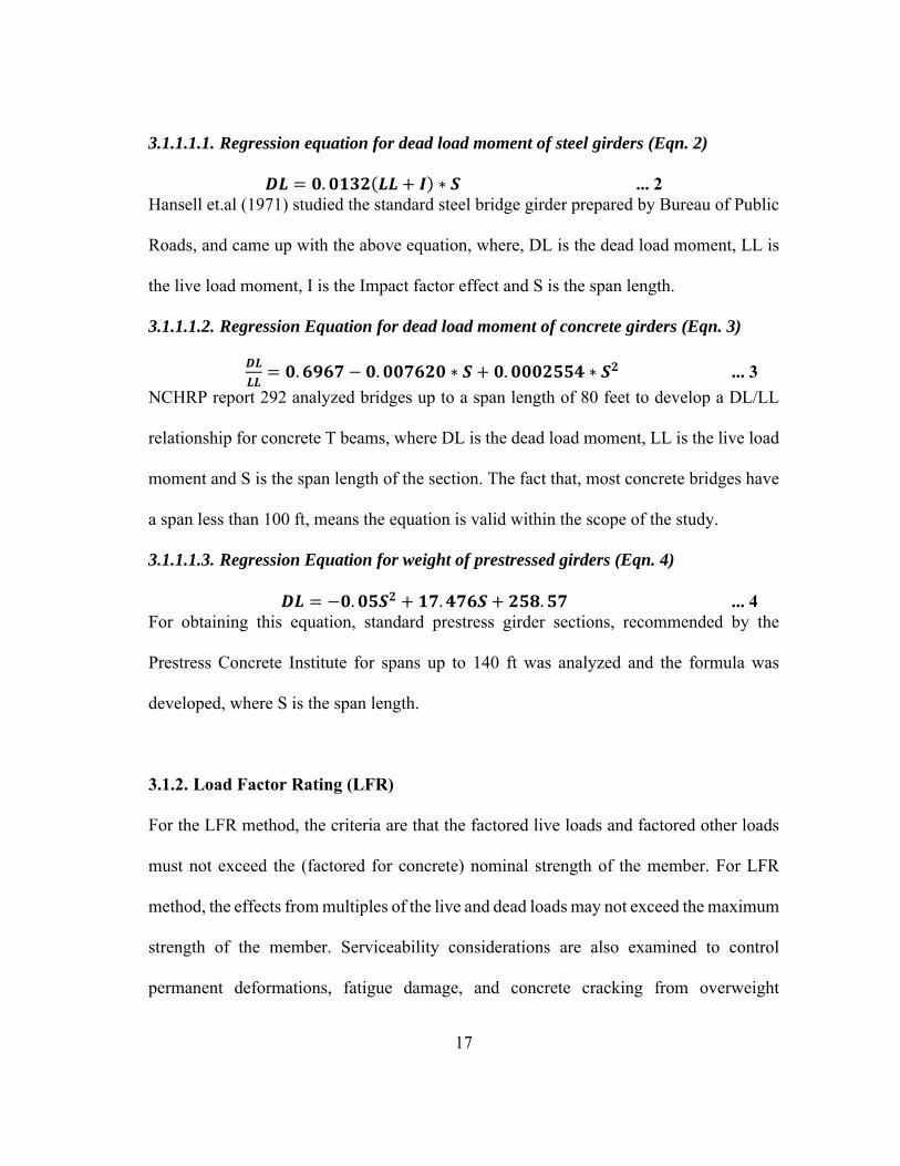
3.1.1.1.1. Regression equation for dead load moment of steel girders (Eqn. 2)

𝑫𝑳 𝟎. 𝟎𝟏𝟑𝟐 𝑳𝑳 𝑰 ∗ 𝑺 ... 2 Hansell et.al (1971) studied the standard steel bridge girder prepared by Bureau of Public

Roads, and came up with the above equation, where, DL is the dead load moment, LL is

the live load moment, I is the Impact factor effect and S is the span length.

3.1.1.1.2. Regression Equation for dead load moment of concrete girders (Eqn. 3)

𝑫𝑳

𝑳𝑳𝟎. 𝟔𝟗𝟔𝟕 𝟎. 𝟎𝟎𝟕𝟔𝟐𝟎 ∗ 𝑺 𝟎. 𝟎𝟎𝟎𝟐𝟓𝟓𝟒 ∗ 𝑺𝟐 ... 3

NCHRP report 292 analyzed bridges up to a span length of 80 feet to develop a DL/LL

relationship for concrete T beams, where DL is the dead load moment, LL is the live load

moment and S is the span length of the section. The fact that, most concrete bridges have

a span less than 100 ft, means the equation is valid within the scope of the study.

3.1.1.1.3. Regression Equation for weight of prestressed girders (Eqn. 4)

𝑫𝑳 𝟎. 𝟎𝟓𝑺𝟐 𝟏𝟕. 𝟒𝟕𝟔𝑺 𝟐𝟓𝟖. 𝟓𝟕 ... 4 For obtaining this equation, standard prestress girder sections, recommended by the

Prestress Concrete Institute for spans up to 140 ft was analyzed and the formula was

developed, where S is the span length.

3.1.2. Load Factor Rating (LFR)

For the LFR method, the criteria are that the factored live loads and factored other loads

must not exceed the (factored for concrete) nominal strength of the member. For LFR

method, the effects from multiples of the live and dead loads may not exceed the maximum

strength of the member. Serviceability considerations are also examined to control

permanent deformations, fatigue damage, and concrete cracking from overweight

18

vehicles. The equation used to determine the rating factor (RF) by LFR method is given

below (Eqn. 5). The different parameters defined are determined as mentioned in MBE

2016.

𝑹𝑭 𝑪 𝑨𝟏∗𝑫

𝑨𝟐∗𝑳∗ 𝟏 𝑰 ... 5

3.1.3. Load and Resistance Factor Rating (LRFR)

LRFR was developed as a rating methodology consistent in philosophy with the AASHTO

LRFD Bridge Design Specifications in its use of reliability-based limit states. The goal of

the design philosophy in the AASHTO LRFD is to achieve a more uniform level of

reliability in bridge design. The equation used to determine the rating factor (RF) by LRFR

method is given below (Eqn. 6). The different parameters defined are determined as

mentioned in MBE 2016.

𝑹𝑭 𝑪 𝜸𝑫𝑪∗𝑫𝑪 𝜸𝑫𝑾∗𝑫𝑾 𝜸𝑷∗𝑷

𝜸𝑳𝑳∗ 𝑳𝑳 𝑰𝑴 ... 6

𝛾 , 𝛾 , 𝛾 , 𝛾 are the LRFD load factor for Live load, Dead loads, wearing surfaces

and Permanent loads, respectively. DC and DW are dead load moments due to structural

elements and wearing surfaces. IM is the impact factor and P is the moment due to

permanent loads.

3.2. Rating Levels

In general, there are two different levels used during the rating of road bridges, Inventory

level rating (IR) and Operator level rating (OR). With respect to vehicle loading Inventory

rating can be defined as that vehicle load which can safely utilize a given bridge for an

infinite period of life. Operator rating can be defined as absolute maximum vehicle load

19

that the bridge may be subjected to. Various previous literatures have shown that, bridges

are designed in such a way that inventory level and operator level ratings for design truck

moments are over 1.0. Studies have proven that; bridges have a much higher reserve load

capacity than the design moment capacities. Truck platooning is a revolutionary

innovation which is still in its experimental stages. Also, the large costs involved in

modifying existing trucks to be adaptable for platooning means that, truck platoon may-

not become a common sight till mid 2020`s. The full-scale commercial shift of freight

traffic to platoon and autonomous trucks are expected to occur after 2030 only.

Considering all these factors into account, operator level rating values can be taken with

respect to a platoon.

3.3. NBI Data Elements used

The research involves utilization of NBI data to determine the load ratings of the large

Texas Bridge inventory. The methodology used to determine the load ratings are explained

later. Here the various data elements used in the study are introduced for better

understanding of the subsequent research stages.

1) Year Built (Item code 27)- This data element provides with the year in which the

bridge was constructed.

2) Length of Maximum Span (Item code 48)- This data element provides with the

center-to-center distance between piers, bents, or abutments measured along the

centerline of the bridge. The measurement is obtained in the nearest foot.

20

3) Structure Function (Item code 5.1)- This data element provides with the

information whether the bridge carries road traffic or pedestrian/rail traffic. It is

useful in identification of the road bridges within the inventory.

4) Latitude, Longitude (Item code 16.1 & 17.1)- These data elements provides with

the GPS latitude and longitude of the bridge at the beginning of the bridge in the

direction of inventory. They are useful during exporting of data to Google Earth.

5) ADT (Item code 29)- This data element gives information on the average daily

traffic of vehicles through the bridge. It is useful in determining the importance of

the highway and in turn the probability of incorporation of platoons.

6) Structure Type (Item Code 43.1)- This data element is utilized to identify the type

of member used for a particular bridge. The dead load moment equations are

applied according to the member type. The data element also gives data regarding

the span type of the main span of the bridge. This data is used to differentiate

simple span bridges with multi span bridges.

7) Structural Evaluation (Item code 67)- This data element gives an evaluation of the

structure based on the condition rating of Super-Structure (Item 59), condition

rating of Sub-Structure (Item 60), and the Inventory Rating. The highest structural

evaluation shall be the lowest of condition rating of superstructure and

substructure.

8) Year Reconstructed (Item code 106)- This data element gives information about

whether the bridge has undergone a major reconstruction. For Bridges

21

reconstructed, it has been assumed that the bridge has been strengthened for newer

design standards.

9) ADTT (Item code 109)- This data element gives what percentage of daily traffic

defined in Item 29 is truck traffic. Pickup vans and light delivery trucks are not

included while calculating ADTT.

3.4. Truck types used

In order to do a comprehensive study on how the variation in truck axle configurations

and wheel loadings effect platooning, six different truck types are considered for the

current thesis study. The first truck type AASHTO 3S2 is a representative truck, which is

similar to many commercially used trucks. They have the least gross vehicle weight

(GVW) among the trucks considered and has the longest axle length. Trucks 3S2, ALDOT

type and DELDOT type have the same axle configurations, but different wheel loadings.

This will help in comparing the effect of wheel loading on platooning. Trucks C5, KYTC

and MDOT have axle lengths decreasing with the same GVW, this set allows to study the

effect of decreasing the axle lengths on the live load moments generated due to platooning.

Similar studies conducted on platooning have used the truck C5 for analysis, hence the

results obtained from C5 truck analysis could be used to compare with the outputs of

previous studies. Use of KYTC and MDOT trucks also helps in knowing the impact of

platoons, when shorter trucks carrying heavier loads ply through bridges. Figure 4 is a

visual representation of the various truck axle configurations used in the study.

22

Figure 4: Various truck configurations used in the study

10 k

11’-0”

4’-2” 17’-8” 4’-2”

20 k 20 k 15 k 15 k

10’-0”

4’-0” 22’-0” 4’-0”10 k 15.5 k 15.5 k 15.5 k 15.5 k

11’-0” 4’-0” 22’-0” 4’-0”10 k 17.5 k 17.5 k 17.5 k 17.5 k

FDOT C5: GVW=80 kips

AASHTO Type 3S2: GVW=72 kips

ALDOT Type 3S2_AL (18 Wheeler): GVW=80 kips

11’-0” 4’-0” 22’-0” 4’-0”8 k 20 k 20 k 16 k 16 kDelDOT T540 (DE 5 Axle Semi): GVW=80 kips

12’-0” 4’-0” 10’-0” 4’-0”8 k 20 k 20 k 16 k 16 kMDOT (HS-Short): GVW=80 kips

12’-0” 4’-0” 14’-0” 4’-0”9.6 k 17.6 k 17.6 kKYTC (Type 4): GVW=80 kips

17.6 k 17.6 k

23

4. RESEARCH STUDY

4.1. Research Approach

Texas’s large bridge inventory has an average age of over 40 years. Moreover, most of the

bridges along the highway systems have been constructed in the 1950’s and 1960’s using

predominantly the ASD method and few by the LFD method. The LFD method has been

used for rating on system bridges other than timber bridges since 2000. Over the last 14

years most bridges have been designed using the LRFD method. Risk assessment of

bridges based on its original design methodology can be a cause for significant error.

Hence in this research an equivalent risk-based approach is taken into account, where the

original load ratings are converted to its corresponding LRFR ratings. The approach

followed in this research consists of five stages. Figure 5 shows the visual representation

of various stages in the research.

Stage 1: Background Analysis - Refined load ratings are determined for select existing

bridges and standard bridge designs, by all three methods of rating, to establish

assumptions for future stages.

Stage 2: NBI Data Analysis - The NBI data is filtered to obtain the selection of bridges

most likely to foresee truck platoons. In addition, supplemental analysis was performed

on multi-span steel girder bridges.

Stage 3: Load Rating Analysis – In this stage the obtained approximate inventory ratings

from stage 1 and bridge information from stage 2 is utilized to determine the approximate

operator rating of the bridges in Texas.

24

Stage 4: Risk Assessment - A relative risk index is identified by converting the load ratings

to equivalent LRFR ratings based on the available literature and then applying the effect

of bridge condition.

Figure 5 : Stages of Research

4.2. Stage 1 – Background Analysis

One of the critical assumptions to obtain the estimated truck platoon load ratings is the

original inventory design rating of existing bridges. Actual bridge plans obtained from

TxDOT were studied in detail and approximate inventory and operator rating of different

types of prestressed concrete and steel type bridges were obtained. The data available from

25

various literature was also considered during this stage to obtain an approximate initial

inventory rating to be assumed for the rest of the study. In order to validate the conversion

factors from different design methods to LRFR method, the standard TxDOT girders and

the actual girder plans obtained were analyzed by all three methods of design and the

corresponding design operator ratings were obtained.

4.2.1. Analysis of Prestressed Concrete Bridges

Before the initiation of load rating analysis based on the obtained plans of prestressed

concrete bridges, the standard prestressed girder details for varying span length were

obtained from TxDOT. Girder detail data tables from 2018 were used for the LRFR study.

Similarly, data tables from 1974 and 1965 were used to evaluate prestressed concrete

beams by LFR and ASR method simultaneously. A total of 63 standard Girder data (36

LRFR, 27 LFR/ASR) and 10 (5 LRFR, 5LFR/ASR) actual bridge girders were evaluated

in this section of the study. The LRFR bridges were evaluated according to the provisions

of AASHTO LRFD Bridge Design Specification. LFR bridges were evaluated by

AASHTO Standard Specification for Highway Bridges 1973. ASR bridges were evaluated

using the commonly used 1969 Ultimate Design Criteria of the Bureau of Public Roads

(BPR) criteria. Bridges load rated using LFR and ASR methods were also load rated using

LRFR method to make a comparison with assumed conversion factors. All the bridge

plans were rated for inventory and operator ratings and the ratios were calculated and

compared. In general, the inventory ratings obtained for prestressed girders were much

higher than one. This is mainly due to the fact that, for prestressed girders in most cases,

it is the stress criteria that governs over the ultimate moment capacity criteria.

26

Table 1: Prestressed girder design load rating results

 No: of Girders 

Mean IR Rating 

IR Less Than 1 

IR Less Than 1.35 

Lowest IR 

Rating 

LRFR Standard Plans 

44  1.62  0  1  1.28 

LFR Standard Plans 

12  1.70  0  0  1.50 

ASR Standard Plans 

23  1.67  0  5  1.12 

NCHRP 122  7  1.67  0  0  1.38 

Actual Girders (LRFR) 

5  1.78  0  0  1.57 

Actual Girders (LFR) 

5  2.12  0  0  1.73 

For prestress girders designed by LFR/ASR methods, inventory rating is calculated by

stress criteria as well as by the capacity of section method. For comparison purposes the

LFR standard girders were analyzed by both methods to obtain the inventory rating. While

the average inventory rating obtained by section capacity method was 1.70, the inventory

rating obtained was only 1.13 when tension was prevented in the section. As the tendon

profile is required to accurately estimate the inventory and operator ratings by this method,

the section capacity method is used in further part of the research. From Table 1 it could

be inferred that the average observed inventory level rating for prestressed bridges are of

the range 1.65 to 1.70. A conservative representative IR rating of 1.35 was then chosen

for the further analysis of prestressed bridges based on a 90-percentile standard deviation

of the entire set.

27

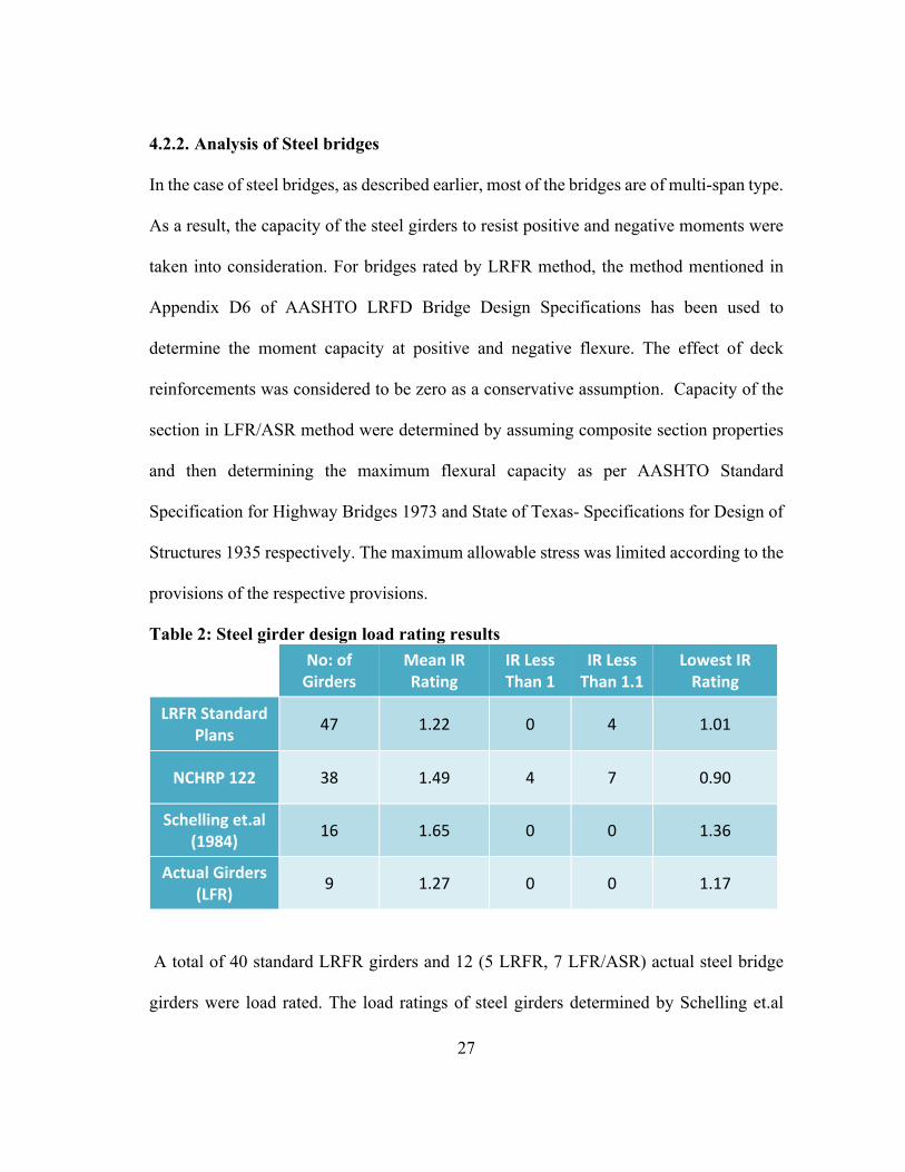
4.2.2. Analysis of Steel bridges

In the case of steel bridges, as described earlier, most of the bridges are of multi-span type.

As a result, the capacity of the steel girders to resist positive and negative moments were

taken into consideration. For bridges rated by LRFR method, the method mentioned in

Appendix D6 of AASHTO LRFD Bridge Design Specifications has been used to

determine the moment capacity at positive and negative flexure. The effect of deck

reinforcements was considered to be zero as a conservative assumption. Capacity of the

section in LFR/ASR method were determined by assuming composite section properties

and then determining the maximum flexural capacity as per AASHTO Standard

Specification for Highway Bridges 1973 and State of Texas- Specifications for Design of

Structures 1935 respectively. The maximum allowable stress was limited according to the

provisions of the respective provisions.

Table 2: Steel girder design load rating results

 No: of Girders 

Mean IR Rating 

IR Less Than 1 

IR Less Than 1.1 

Lowest IR Rating 

LRFR Standard Plans 

47  1.22  0  4  1.01 

NCHRP 122  38  1.49  4  7  0.90 

Schelling et.al (1984) 

16  1.65  0  0  1.36 

Actual Girders (LFR) 

9  1.27  0  0  1.17 

A total of 40 standard LRFR girders and 12 (5 LRFR, 7 LFR/ASR) actual steel bridge

girders were load rated. The load ratings of steel girders determined by Schelling et.al

28

(1984) and NCHRP Report 122 were also considered. Table 2 shows the obtained mean

IR ratings by actual study and literature study. Based on the mean and standard deviation

obtained a 90th percentile IR rating of 1.10 was fixed for further analysis and design.

4.2.3. Stage 1 Findings

From the analysis of bridge girder plans, it was observed that for all the girders considered,

the design inventory rating based on the girder capacities, is much higher than one for both

steel prestressed concrete girders. Hence the initial assumption of inventory rating of one

for all bridges is modified. The mean and standard deviations of inventory ratings for steel

and prestressed concrete bridges are determined and a 90% confidence interval is

considered. The initial inventory ratings assumed for the further stages of the study are

1.35 for prestressed concrete bridges and concrete bridges and 1.10 for steel bridges.

4.3. Stage 2 – NBI Data Analysis

The second stage of the study involves filtering of the available NBI data to relevant data

sets and bridges. As described earlier, Texas has a large inventory of nearly 55,000 bridges

of which nearly more than half the bridges are located along by roads, through which

platoons may never travel through. In the TxDOT NBI data inventory, information

regarding STRAHNET status of each bridge is available. STRAHNET refers to the

Strategic Highway Network of the United States, which comprises mainly of the interstate

highways, their feeders and connection roads to ports, airports and military installations.

These roads are highly likely to witness truck platoons in the immediate future and are

29

those considered in this study. This helps in further reducing the data set to nearly 8,000

bridges. In order to refine further, bridge with a span less than 50 feet are ignored. This is

done based on the fact that, in most cases a minimum span length of 60 feet is required to

produce live load platoon moments greater than that caused by a single truck passing

through the same bridge. Bridges with daily truck traffic less than 100 are also filtered out.

These filtering maneuvers reduces the total number of analysis bridges to 6,550. Further

filtering is done to remove timber bridges, arch bridges and other similar types of special

bridges (Item 43.1- member type 41-99). This is done because in most of the cases, the

design of these bridges are different from the standard procedures and would require

specific inventory level analysis to know their capacity and live load behaviors, which are

beyond the scope of the study. This further reduces the number of bridges to 6,100.

From the NBI data analysis it was observed that more than 60 % of the steel bridges have

a multi span configuration. From the NBI data, details regarding the maximum span length

and number of main spans can be obtained. The information regarding each span length

for multi-span bridges or the number of spans in each continuous span is not available.

Since there are over 1850 multi-span steel bridges, an assumptive method was used to

determine the effective live load effects of truck platooning on multi-span bridges. For

both LRFD and LFD bridges, it was observed that the impact of maximum negative

moment variation is much higher than the maximum positive moment variation. It was

assumed that, the maximum span length is the span of all sections within the continuous

bridge and the number of main spans were assumed to be the number of continuous spans

in a unit. SAP 2000 software was used to do the multi-span analysis. Analysis was done

30

for the 6 trucks considered and for 3 different truck spacing’s of 25, 30 and 40 feet’s

respectively. The ratio of maximum live load moment due to the platoon and the design

live load was calculated for maximum positive and negative moments. The ratio values

where determined for span lengths varying from 50 to 175 feet and number of spans

varying from 2 to 4. Based on the analysis results, equations were developed to represent

the ratio variation along span length for each truck type at a particular truck to truck axle

spacing.

From the multi-span analysis for truck platoons, it was observed that the maximum

moment diagrams for truck platoons, varied significantly from that of design trucks. The

fact that platoons are live load trains of length range 150 to200 feet means that, for multi-

spans the platoons are contained entirely within the bridge spans and hence producing

greater live load moments at the midspan and support regions. The negative moments

generated at support regions in multi span bridges where observed to be similar to the

maximum moment for the simply supported case for many span length and truck

configuration cases. Based on the above two observations, it was decided to limit multi-

span effect consideration to a maximum span length of 175 feet for each multi-span girder.

For bridges having maximum span length greater than 175 feet, it is assumed that the

moment generated is equal to the maximum simply supported span moment. A sample

moment ratio output of multi-span study is shown in Appendix B

31

4.4. Stage 3- Load Rating Analysis

Based on the filtered bridge data, load rating analysis was performed to calculate an

approximate load rating for the filtered STRAHNET bridges in Texas for various truck

platoon configurations. An Excel tool and a MATLAB tool were developed to do the load

rating analysis. For multi-span bridges live load moments were calculated using SAP2000

software and the results were added to the Excel and MATLAB tool as coefficients, which

are described later.

Considering the large size of the available bridge inventory to be assessed, a simplified

approach has been taken for the load rating procedure. Assumptions have been made in

such a way that it satisfies a broad spectrum of the bridge inventory to be analyzed. The

assumptions made were:

1) All the prestressed concrete girder bridges are assumed to be simply supported.

This span configuration is used by 98% of prestressed girder bridges within Texas.

Even though the bridge decks may be continuous, the beams are still simply

supported and hence the rotational restraint at the supports is negligible.

2) More than 60% of the steel bridges have a continuous span, hence a modified

moment calculation procedure has been followed, as explained earlier.

3) The inventory rating of all the bridges are assumed based on the analysis

performed in Stage 1. For this research it allows for determination of the capacity

of the bridge.

4) Impact factor for truck platooning and for design trucks are assumed to be the

same.

32

5) The effect of age deterioration, potential loss of capacity due to fatigue or other

causes are only considered through the NBI structural condition rating.

6) It is assumed that only the platoon trucks are on the bridges. That is, the lane

loading effect due to smaller vehicles is ignored while determining operator

ratings.

7) It is assumed that flexure controls the load ratings. Historically most bridge

designers ensured that shear did not control.

For both LFR and LRFR rating methods, the numerator in the rating equation is

assumed to be constant (shown in Equation 7 and 8), as the dead loads and capacity

remain a constant for both operator and inventory rating methods under all general

conditions. Where A is a constant equivalent to ultimate capacity minus the

factored dead load moments acting on the section of the bridge.

𝑹𝑭𝑳𝑭𝑹𝑨

𝑨𝟐∗𝑳∗ 𝟏 𝑰 ... 7

𝑹𝑭𝑳𝑹𝑭𝑹𝑨

𝜸𝑳𝑳∗ 𝑳𝑳 𝑰𝑴 ... 8

8) For ASR method, the stress levels used to determine bridge capacity is different

for inventory (55 percent yield) and operator (75 percent yield) ratings. Hence the

inventory level capacity of the bridge is found approximately as the sum of design

live load moment including the effect of impact loading plus the moment due to

dead loads (based on the assumption IR is one). The obtained capacity is then

multiplied by a factor 1.36 (0.755/0.55) to obtain the approximate capacity at

operator level.

33

4.4.1. VBA Program Flow Procedure

An Excel tool developed capable of analyzing up to five truck platoons of any axle

configuration and truck-to-truck spacing was developed. The Visual Basics for

Applications (VBA) programming language platform available within Excel has been

used to automate the analysis and output generation. Excel macro codes were used within

VBA to repeat the given inputs for all the bridges and obtain the output result. The bridges

are identified by their Freight Corridor number. Freight Corridor number refers to the

designated highway number allocated to different routes within Texas by TxDOT. The

direct corridor number data is not available from NBI data; hence ArcGIS software is used

to obtain the same. A map layer of Texas Freight Corridors is overlapped over the Texas

bridges layer map. The data is clipped based on the bridge ID and saved as an Excel file,

which is then added to the Excel tool. In order to facilitate easier determination of the load

rating data of the bridges after filtration, the following program flow procedure has been

utilized:

1) Input the Bridge Id/Route Number, truck axle configuration and number of trucks

in the platoon.

2) Identify the bridge based on its Bridge Id/Route number using the NBI data.

3) Record max span length, year constructed/reconstructed and structure type data of

the bridges.

4) Determine the method used for design of the bridge based on the year of

construction (ASD/LFD/LRFD).

34

5) Determine the maximum design live load moment using the corresponding design

truck and maximum span length.

6) Determine the capacity of the LFD and LRFD bridges using the assumed inventory

rating and structure type. For ASD bridges determine the capacity using the

estimated expressions described earlier

7) Determine the maximum live load moment due to the truck platoon load

configuration entered.

8) Determine the operator rating of the bridge for platoon trucks.

Figure 6 is a flow diagram of various steps involved in stage one of the research

Figure 6: Flow diagram of Steps in Stage 1

4.4.2. MATLAB Analysis

In order to facilitate faster analysis of all the bridges simultaneously, a MATLAB program

was developed. The program follows a similar coding flow as the VBA code. In order to

facilitate faster calculations, three separate spreadsheets where linked to the MATLAB

code. The first sheet consisted of the NBI select data element details and the second sheet

35

consisted of moment data for spans 40-500 feet at 5 feet intervals for all the truck

combinations and spacing considered for the study. The moment values were pre-

determined to reduce the computation time. The third sheet consisted of the various

moment ratios to be used for the multi-span analysis. Conditional loops were used to

segregate bridges based on span type, age and material. The outputs were printed on to

another spreadsheet file for easier post analysis. The MATLAB code used in the study is

shown in Appendix C

4.4.3. Initial Results

Figure 7 and Figure 8 are samples of data analysis results for LRFR and LFR methods

based on the entire Texas Bridge Inventory. The graphs show the operator rating by LRFR

and LFR rating methods for 2 truck C5 platoons at an axle-to-axle spacing of 30 and 40

feet respectively. The number of bridges in each span range are also shown, for better

understanding of the data. It is to be noted that, for a platoon configuration with the

increase in span length, the rating factors decreases initially and then increase after a

threshold span length. From the figure, it can be seen that for both old and new bridges,

most of the bridges have a maximum span length less than 140 feet, the commonly used

maximum length of a prestressed concrete girder bridges.

36

Figure 7: Sample analysis data graph for bridges built by LRFD method

Figure 8 : Sample analysis data graph for bridges built by LFD method

978

765

868

731660 690

11281060

318

13891

47 26 28 22 27 39 40 42

125

0.80

1.00

1.20

1.40

1.60

1.80

2.00

0

200

400

600

800

1000

1200

Rating Factor

No: o

f Bridges

Span Length (ft)

2 Truck C5‐ bridges built 2005‐2018

Bridges

30 ft spacing

40 ft spacing

1631

852

1478

861800

619

894

603

13061 45 32 34 20 28 17 22 33 15

64

0.80

1.00

1.20

1.40

1.60

1.80

2.00

0

200

400

600

800

1000

1200

1400

1600

1800

Rating Factor

No: o

f Bridges

Span Length (ft)

2 Truck C5‐ bridges built 1975‐2004

Bridges

30 ft spacing

40 ft spacing

37

Figures 9 to 12 are a comparison of the platoon to design truck moment ratios with bridge

span length for different platooning configurations. All truck types irrespective of the

platoon configuration has a constant moment ratio up to a span length of 90 feet (90 feet

can be considered the minimum bridge length required to generate excess moments due

to platooning). For both 3S2 and C5 type trucks, when compared to LRFR bridges, the

moment ratio obtained is below 1.0, hence the subsequent operator ratings will be well

above 1.0. Whereas the moment ratios obtained when compared to HS20 (LFR) design

trucks are more than 1.0 and hence, it is likely that the operator ratings obtained on analysis

may be less than 1.0. From the comparison graphs it can be concluded that bridges built

prior to 2004 (LFR/ASR) are more susceptible to overload failure due to the crossing of

platoons, especially if they do not have good structural condition, It is observed that for a

particular truck, the effect of 2 and 3 truck platoons are constant up to a certain span length,

beyond which they diverge. For 3S2 type trucks, for a spacing of 30 ft between trucks, the

effect of 2 and 3 trucks are same up to a span length of 155 ft. Considering the fact that

most of the bridges within Texas Inventory have a span length less than 150 ft, the effect

of 2 and 3 truck platoons will be same for 3S2 trucks in most conditions.

38

Figure 9 : Graph showing variation of the 3S2 truck moments with respect to HL93 design moments.

Figure 10 : Graph showing variation of the C5 truck moments with respect to HL93 design moments.

0.50

0.55

0.60

0.65

0.70

0.75

0.80

0.85

40 60 80 100 120 140 160 180 200

Truck/H

L93 M

omen

t Ratio

Span Length

TYPE 3S2 TRUCKS

2 Truck 30ft 2 Truck 40ft 2 Truck 50ft

3 Truck 30ft 3 Truck 40ft 3 Truck 50ft

0.60

0.65

0.70

0.75

0.80

0.85

0.90

0.95

40 60 80 100 120 140 160 180 200

Truck/H

L93 M

omen

t Ratio

Span Length

TYPE C5 TRUCKS

2 Truck 30ft 2 Truck 40ft 2 Truck 50ft

3 Truck 30ft 3 Truck 40ft 3 Truck 50ft

39

Figure 11 : Graph showing variation of the 3S2 truck moments with respect to HS20 design moments.

Figure 12: Graph showing variation of the C5 truck moments with respect to HS20 design moments.

0.65

0.75

0.85

0.95

1.05

1.15

1.25

1.35

40 60 80 100 120 140 160 180 200

Truck/H

S20 M

omen

t Ratio

Span Length

TYPE 3S2 TRUCKS

2 Truck 30ft 2 Truck 40ft 2 Truck 50ft

3 Truck 30ft 3 Truck 40ft 3 Truck 50ft

0.85

0.95

1.05

1.15

1.25

1.35

1.45

40 60 80 100 120 140 160 180 200

Truck/H

S20 M

omen

t Ratio

Span Length

TYPE C5 TRUCKS

2 Truck 30ft 2 Truck 40ft 2 Truck 50ft

3 Truck 30ft 3 Truck 40ft 3 Truck 50ft

40

4.5. Stage 4- Risk Assessment

In this stage of risk assessment, the obtained operator ratings are then converted to the

corresponding load rating by the LRFR method for all bridges, irrespective of their

original rating method and method of design. FHWA is currently under the process of

converting all load ratings of on-system bridges to LRFR bridges. Hence, in order to be at

consensus with the process, ratings obtained by LFR and ASR method are converted to

LRFR ratings based on conversion factors, described in the following section.

4.5.1. LFR to LRFR Conversion

Due to the unavailability of exact bridge data to load rate by both methods, similar studies

conducted by other authors has been referenced to obtain the conversion factors. NCHRP

Report 122 (2005) and NCHRP Report 700 (2011) are two studies that were conducted in

order to compare the load rating variation of bridges by LFR and LRFR methods. Both

the studies are of similar nature in which, the load ratings where done analytically using

AASHTO Bridge rating software’s VIRTIS and AASHTOWARE, respectively.

NCHRP 122 report focuses on providing a comparison between ratings generated by

LRFR method and LFR methods. The comparisons were based on flexural strength and

only the interior girders were considered. 74 representative bridge plans obtained from

NYSDOT and WYDOT were analyzed in the study to obtain the comparison. The study

included 44 steel plate girder/rolled beam bridges and 17 prestressed girder type bridges.

All the bridges were load rated at inventory and operator level using design trucks as well

41

as type 3S2 trucks. From the study it was also observed that, for all the bridges analyzed

the inventory level load rating was greater than 1.0, validating the initial assumption.

NCHRP 700 involved an extensive of study of bridge load ratings which included bridges

from 8 states. Detailed bridge data of 18,037 bridges were collected. 1,500 bridges with a

total of 3,043 girder sections where analyzed in detail for 12 vehicle combinations each.

The filtration of the bridges to 1,500 was done in such a way that, it represented all the

commonly used type of bridge types in United States, with bridges from different periods

of constructed, ensuring it is a highly representative set of American bridge inventory. A

total of 704 prestressed girders and 1,430 steel multi-girders were analyzed as a part of the

study. In the analysis section shear and moment ratings of the different types of girders

were compared by LFR and LRFR inventory rating as well as a reliability study was also

conducted. From the data analysis of the in-depth report of the study, it was observed that

only 12 (1.7%) out of the 704 prestressed I-girders had a LFR rating less than 1.0.

Similarly, there were only 70 (4.9%) steel girders with a LFR rating than 1.0.

The data from both documents have been taken together and a weighted average has been

used to obtain the final conversion factor from LFR to LRFR. The factors are shown in

Table 3

42

Table 3: LRFR conversion factors

Rating Method LRFR Conversion Factors

Steel Bridges Concrete Bridges

LRFR 1.00 1.00

LFR 0.77 0.50

ASR 0.88 0.47

4.5.2. ASR to LFR Conversion

Similar to the conversion of LFR to LRFR ratings, bridges rated by ASR method had to

be converted to LRFR rating. Direct literature reference on conversion of ASR to LRFR

ratings was not obtained, hence factors were determined to convert ASR ratings to LFR

ratings based on available literatures. Then the conversion from LFR to LRFR was

performed in the manner illustrated in the earlier section.

Schelling et.al (1984) compared the load rating values of 16 steel girder type bridges in

Maryland by LFR, ASR and Auto Stress method of rating. 8 bridges were of simple span

type while the remaining bridges where multi-span type. The authors also developed a

regression equation to convert ASR ratings to LFR ratings. From the study it was observed

that the average rating by LFR was more than ASR method for steel bridges by about 16

%. The inventory level ratings were observed to vary between 1.2 and 1.6 for all the

bridges.

In MCHRP Report 91-1 (1994) 73 bridges (33 Concrete & 40 Steel bridges) were load

rated by LFR, ASR and Strength method of rating. The bridges used for study were bridges

that were identified as bridges that required posting or were on the verge of being posted

43

based on ASR method. Due to this fact, the average inventory rating observed for the

bridges was less than one. For steel bridges, the observed LFR ratings were higher than

ASR ratings, while for concrete bridges, ASR ratings were higher.

The data from both literatures has been taken together and weighted average method has

been used to obtain the final conversion factor from ASR to LFR. The factors are shown

in Table 3.

Table 4 shows the operator rating obtained by analysis of the obtained prestressed girder

plans by all the three methods of rating. Bridges constructed by ASR and LFR methods

were rated by all three methodologies. Older bridges showed a lower operator rating due

to the fact that ASR and LFR bridges were designed for HS20 loading while LRFR bridges

were designed for the much higher HL93 loading. The ratios obtained are slightly higher

than the values obtained based on literature reference. Hence the literature values can be

considered conservatively.

Table 4: Operator Rating ratio obtained by actual plans

Design Rating Method Operator Rating

𝑳𝑹𝑭𝑹 𝑶𝑹𝑫𝑬𝑺𝑰𝑮𝑵 𝑶𝑹

 ASR LFR LRFR

ASR 2.73 2.79 1.62 0.59

LFR 2.82 2.89 1.65 0.57

LRFR - - 2.12 1

44

4.5.3. Application of NBI Condition Ratings

Upon obtaining the equivalent LRFR operator ratings for each bridge, possible reduction

in capacity due to age or other factors are taken into account by applying the effect of

bridge condition. Due to the large size of data set to be considered, individual assessment

of each bridge is not possible. NBI data includes a data attribute called structural

evaluation rating, which as described earlier is a direct indicator towards the condition of

each bridge. NBI coding manual describes how to interpret the corresponding effective

bridge load rating based on its structural evaluation rating.

Table 5: Appraisal Evaluation Rating factor

The manual defines the maximum permissible truck load that can traverse through the

bridge based on its appraisal rating. In the current research study, the truck loads converted

to equivalent rating multiplication factors. The conversion is done by dividing the

allowable load by the original design load for which the bridge was designed. Table 5

gives the multiplication factors used to convert the obtained operator ratings from Stage 3

to the effective operating rating (EOR) taking into account bridge condition.

4.6. Bridge Prioritization

After completion of load rating analysis, the bridges were prioritized according to their

equivalent operator rating (EOR). Prioritization of the bridges help in the identification of

high priority routes based on the relative risk. Five priority levels were developed. Level

1 priority bridges has the lowest level of relative risk and are unlikely to have any issues

Appraisal Rating >7 7 6 5 <5

Multiplication Factor 1 0.85 0.75 0.60 0.50

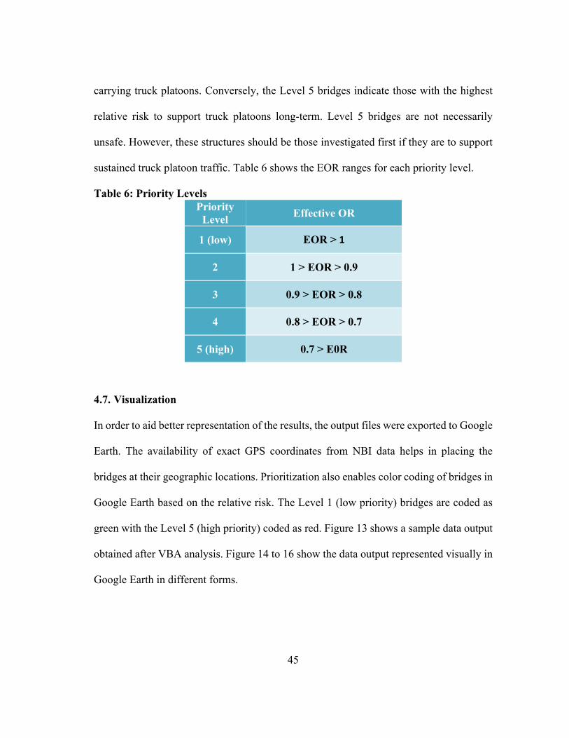
45

carrying truck platoons. Conversely, the Level 5 bridges indicate those with the highest

relative risk to support truck platoons long-term. Level 5 bridges are not necessarily

unsafe. However, these structures should be those investigated first if they are to support

sustained truck platoon traffic. Table 6 shows the EOR ranges for each priority level.

Table 6: Priority Levels Priority

Level Effective OR

1 (low) EOR > 1 

2 1 > EOR > 0.9

3 0.9 > EOR > 0.8

4 0.8 > EOR > 0.7

5 (high) 0.7 > E0R

4.7. Visualization

In order to aid better representation of the results, the output files were exported to Google

Earth. The availability of exact GPS coordinates from NBI data helps in placing the

bridges at their geographic locations. Prioritization also enables color coding of bridges in

Google Earth based on the relative risk. The Level 1 (low priority) bridges are coded as

green with the Level 5 (high priority) coded as red. Figure 13 shows a sample data output

obtained after VBA analysis. Figure 14 to 16 show the data output represented visually in

Google Earth in different forms.

46

Bridge ID Highwa

y District

Span

Year Built/

Rebuilt Bridge Category

Operator Rating

Net OR

Priority Index

100930049507254 10 65 1966 prestress concrete

girder2.81 1.12 1

100930049507256 10 65 1966 prestress concrete

girder2.81 0.99 2

100930049507279 10 70 1967 steel girder 1.52 0.88 3100930049507280 10 45 1987 concrete bridge 3.23 0.96 2102120049505177 10 95 1964 steel girder 1.61 0.74 4

102120049506239 10 65 1966 prestress concrete

girder2.81 0.79 4

102340049502010 10 60 1963 steel girder 1.61 0.74 4

102340049502312 10 95 2000 prestress concrete

girder2.55 1.07 1

102340049503001 10 75 2005 prestress concrete

girder3.01 2.56 1

102340049503096 10 45 1962 steel girder 1.92 0.89 3

100930013801122 10 80 2005 prestress concrete

girder3.01 2.56 1

102120049504054 10 70 1961 steel girder 1.52 0.88 3

Figure 13 : Sample output obtained on VBA analysis

Figure 14 : Google Earth visualization of high priority bridges for type 3S2 trucks under 3 truck, 30 feet spacing combination

47

Figure 15 : Google Earth visualization of a color-coded section of Inter-State near Hillsboro, Tx

Figure 16 : Google Earth visualization of color-coded section of Inter-State near Hillsboro, Tx with a bridge selected

48

5. ANALYSIS INTERPRETATIONS

In order to aid better representation of the outcomes, the results are presented separately

based on the three governing parameters: truck spacing, bridge span length, truck type and

number of trucks in the platoon. In addition, the prestressed girder and steel girder bridge

results were compared. Each are presented separately below.

5.1. Impact Based on Truck Spacing

Figure 17 shows the variation in the percent of high priority (Level 5) bridges obtained on

analysis of the 6,550 STRAHNET bridges. For all the truck types, the largest percentage

of high priority bridges were obtained for a truck axle-to-axle configuration of 25, 30, 40

and 50 feet. For all the trucks, the variation is roughly parabolic with respect to increase

in truck spacing. The percentage of high priority bridges decreased by 23 %, 45 % and 56

% on an average when the truck spacing increased from 25 to 30, 40 and 50 feet

respectively. There are several reasons as to why the percentage of high priority bridges

do not go to zero. It was observed that about 30 % of the high priority bridges for each

truck type were independent of the platoon spacing and dependent only on the truck type.

This is due to the fact that more than 15 % of the total bridge inventory considered has a

maximum span length less than 75 feet, and hence two trucks being on top of the bridge

together is not possible. The consideration of the structural condition factors is also a

reason behind a fixed minimum percentage of high priority bridges irrespective of the

platoon spacing.

49

Figure 17 : Variation of percentage of high priority bridges with platoon spacing

Figure 18 is a visual representation of how the number of bridges in each priority category

change with the condition applied. C5/3S2 refers to the truck type, 3 refers to the number

of trucks in platoon and 30/50 refers to the spacing between the trucks (30 ft or 50ft). It is

to be noted that 3S2 truck type at a spacing of 50 ft is almost representative of the exiting

road conditions when two trucks cross a bridge with a close spacing. While C5 truck type

at a spacing of 30 feet is representative of a future heavier tuck type moving in a platoon

spacing of 30 feet.

0

5

10

15

20

25

30

35

25 30 35 40 45 50

% High Priority

Axle to Axle Spacing Between Trucks

Variation of Level 5 Priority Bridges with Truck Spacing

3S2 ALDOT C5

DELDOT KENTUCKY MDOT

50

Figure 18: Bar charts showing the variation in higher priority bridges for 3S2 and C5 for 30 ft and 50 ft spacings

0

500

1000

1500

2000

2500

Bridges

C5 3 30

1 2 3 4 5

0

500

1000

1500

2000

2500

Bridges

3S2 3 30

1 2 3 4 5

0

500

1000

1500

2000

2500

Bridges

C5 3 50

1 2 3 4 5

0

500

1000

1500

2000

2500

Bridges

3S2 3 50

1 2 3 4 5

51

5.2. Impact Based on Span

Simple span and multi-span conditions has been considered during this study. In order to

get a better understanding about the impact of platoons on multi span bridges, a

comparative study between single span and two-span bridges was performed. Figure 19

and Figure 20 shows the variation of C5 truck operator ratings for different span lengths.

In the figures, SS refers to single span and MS refers to multi-span bridges. Similarly,

EOR LFR refers to the equivalent operator rating of the bridge by LRFR method, i.e. the

operator rating after making LFR to LRFR conversion.

Figure 19 : Comparison of simple span and multi span Operator Rating with span length for 3 C5 truck platoons

0.80

1.00

1.20

1.40

1.60

1.80

2.00

2.20

50 60 70 80 90 100 110 120 130 140 150

Operator Rating

Span Length (ft)

LRFR & LFR Operator Rating ‐3 truck 30ft C5 platoon

LRFR SS LFR SS EOR LFR MS

LRFR MS LFR MS EOR LFR SS

52

Figure 20 : Comparison of simple span and multi span Operator Rating with span length for 2 C5 truck platoons

It can be seen from the figure that, even though there is a reduction in design moments,

for multi-span bridges, there is a significant drop in operator ratings for multi span bridges

when compared to simple span bridges. This is mainly due to the fact that, when platoons

are considered, more than two bridges are present in the span of the bridge at any given

time, hence producing much higher negative moments than that is generated due to the

combined design truck and lane loading. The operator ratings for multi-span sections

shows a decreasing trend over span lengths of 150 feet, mainly due to the fact that, the

0.80

1.00

1.20

1.40

1.60

1.80

2.00

2.20

50 60 70 80 90 100 110 120 130 140 150

Operator Rating

Span Length (ft)

LRFR & LFR OPERATOR RATINGS FOR 2 TRUCK 30 FT C5LRFR SS LFR SS EOR LFR MS

LRFR MS LFR MS EOR LFR SS

53

effective bridge length exceeds the platoon length significantly, and since lane loading is

not considered, the platoon moment effect increase gets reduced.

5.3. Impact Based on Truck Type

Figure 21 show the variation in number of STRAHNET bridges when the truck type

changes for different platoon spacings for 3 truck platoon’s configurations. The specific

trucks with their axle spacing and weights were provided earlier in Figure 4 Type 3S2,

ALDOT and DELDOT type trucks have the same truck axle configuration with different

wheel loadings. Type 3S2 has the least percentage of high priority bridges as 3S2 has the

least GVW among those considered. This indicates that, the impact of truck type on

platoons is related to the truck GVW. The higher the GVW, larger the percentage of high

priority bridges. Whereas even though ALDOT and DELDOT type trucks have the same

GVW (80 kip) and axle configuration, the percentage of high priority bridges is

significantly higher for DELDOT trucks. This can be the attributed to the difference in

load distribution among the axles. The highest singles axle load in a DELDOT type truck

is 20 kip compared to 17.5 kip in ALDOT truck and 15.5 kip in a 3S2 type truck. The

comparison of the three truck types conveys that determination of a high priority bridge

in a route, depends on the truck axle configuration, GVW and the axle load distribution.

Type C5, KENTUCKY and MDOT trucks all have 80-kip GVW, with decreasing distance

between the front and rear axles. The percentage of high priority bridges doubles when

the axle spacing between the front and rear axles decrease from 17’8’’ to 10’. This means

54

that, shorter trucks, carrying very heavy loads are more prone to overload bridges when

compared to longer trucks.

Figure 21: Variation of high priority bridges by truck type and spacing for 2 truck platoons

5.4. Impact Based on Trucks within a Platoon

In order to compare the impact of the number of trucks in a platoon, a comparative study

was performed with 2 and 3 trucks. Upon comparison it was observed that the number of

high priority bridges increased by less than 15 % when the number of trucks in platoon

increased from 2 to 3. Even though the net increase in moment for 3 truck platoons higher

for longer span lengths, nearly 80 percentage of the inventory has a span length less than

150 feet, hence minor rise in high priority bridges. Table 7 and Table 8 compare the 3

truck and 2 truck data outputs under different truck spacing for different truck types.

0

5

10

15

20

25

30

35

3S2 ALDOT DELDOT C5 KENTUCKY MDOT

% High Priority

Truck Type

Variation of High Priority Bridges by Truck Type 

25FT 30FT 40FT 50FT

55

Table 7: 3 truck platoon 30 feet vs 40 feet comparison

Priority Level 

 3 truck 30 feet spacing  3 truck 40 feet spacing 

3S2  ALDOT  C5  3S2  ALDOT  C5 

1  3460  2426  1644  4088  2573  1698 

2  1487  964  884  1373  1454  1087 

3  649  1568  1298  308  1457  1643 

4  483  847  1543  366  439  1202 

5  169  443  879  113  325  618 

Table 8: 2 truck platoon 30 feet vs 40 feet comparison

Priority Level 

2 truck 30 feet spacing  2 truck 40 feet spacing 

3S2  ALDOT  C5  3S2  ALDOT  C5 

1  3620  2565  1693  4119  2655  1793 

2  1382  985  999  1375  1403  1058 

3  655  1470  1337  292  1451  1612 

4  429  852  1407  353  415  1190 

5  162  376  812  109  324  595 

56

5.5. Steel Versus Prestressed Girder Bridges

A comparison study between prestress and steel type bridges for different truck and

spacing configurations was also conducted. For trucks with lesser GVW, the percent of

prestressed bridges under the least priority category is less than that for steel bridges. For

trucks heavier than C5, the percentage of bridges under least priority falls significantly

below steel bridges for prestress bridges. The variation is parabolic for steel bridges, with

the highest fall observed between C5 and 3S2 type trucks. No correlation was observed

for variation in platoon and spacing configuration.

Table 9: 2 truck platoon steel vs prestress girder comparison

Priority Level 

2 truck platoon at 40 feet spacing 

3S2‐ Steel ALDOT‐Steel 

C5‐Steel 3S2 ‐

Prestressed ALDOT‐ 

Prestressed C5‐

Prestressed 

1  989  723  671  3130  1932  1122 

2  440  266  121  935  1137  937 

3  28  440  308  264  1011  1304 

4  109  38  347  244  377  843 

5  9  108  128  100  216  467 

The increase in high priority bridges with reduced span length follows a similar pattern in

both steel and prestress bridges. The significant variation in prestress low priority bridges

with truck type is mainly due to the fact that, a good percentage of the prestress highway

bridges were constructed during the Interstate era in late 1950s and were designed mainly

to resist HS20 live loading only. Hence, lesser design moment capacity, along with

deterioration effects makes prestress bridges highly susceptible for heavier platoon

57

loading combinations. Table 9 and Table 10 shows the comparison between prestress and

steel bridges for 3S2, ALDOT and C5 trucks under 2 and 3 truck platoons at 40 spacing.

Table 10: 3 truck platoon steel vs prestress girder comparison 

Priority Level 

3 truck platoon 40 feet spacing 

3S2‐ Steel 

ALDOT‐Steel 

C5‐Steel 3S2 ‐

Prestressed ALDOT‐ 

Prestressed C5‐

Prestressed

1  960  641  576  3128  1932  1122 

2  448  319  152  925  1135  935 

3  37  448  350  271  1009  1293 

4  119  58  354  247  381  848 

5  11  109  143  102  216  475 

58

6. FUEL SAVINGS STUDY

The output files from Stage 4 were exported to ArcGIS for an approximate cost benefit

analysis study. The focus was on implementation of truck platoons along particular routes

as well as Texas as a whole. The detailed ArcGIS analysis procedure is mentioned in the

following section.

At first TxDOT Roadway Inventory 2016 GIS map containing 640,000 data entries was

downloaded from the TxDOT website. The map contains the data of all road segments in

Texas. Each road segment has 152 column attributes, corresponding to various structural

and traffic conditions. A definition query SEC_STR =1 OR SEC_STR_CON =1 was

applied to filter out the STRAHNET highways of Texas. The application of filter reduces

the number of data entries to 11300, representing a total distance of 6200 miles.

The TxDOT bridge file containing 55,000 entries was downloaded and added to ArcMap

file. The file contains details regarding maximum span, year constructed and the structural

evaluation rating of the bridges. The definition query STRAHNET_HWY_DSGNAT = 1

was applied to filter out the STRAHNET classification bridges. The data was then

exported to Microsoft Excel using the export to xls. tool within the ArcMap Toolboxes.

The output from the earlier MATLAB analysis was saved as an Excel file and was added

to the existing bridge data. The data was then imported back to the ArcMap file. The

imported Excel file was then converted to a XY data projection with

GCS_North_American_1983 coordinate system. The projection was saved as a map layer.

59

Necessary definition query was applied to obtain the high priority (Level 5) bridges. The

Buffer tool was then utilized to fix a buffer distance around each high priority bridge. The

buffer zone was the stretch of roadway in which the platoon system should move at a

higher spacing between each other to ensure the safety of the bridge. The buffer radius is

fixed at one-mile distance upstream and downstream of the bridge. Most bridges in Texas

have a length of less than half a mile and the one-mile radius giving a fairly accurate

representation (higher buffer length of 1.5 miles will be tried to compare the changes).

The dissolve function was then used to accommodate for the overlapping buffers.

Fields were added in the TxDOT Roadway attribute tables to determine the annual fuel

consumption and fuel savings per segment of the roadway. An average fuel consumption

of 6 miles per gallon was assumed for trucks based on the data obtained from various

sources. The attribute data provided with data of section length and number of trucks

passing through that roadway section in a day. These values were multiplied to obtain the

annual fuel savings. It was assumed that all the trucks going through the road at present

truck traffic levels will be in a platoon. The fuel savings were determined based on the

various literature studies done in the prior parts of the report. The fuel consumption rate

is taken at 6 mpg based on data obtained from U.S. Energy Information Administration

(eia.gov). The Erase tool was then used to erase the roadway map layer with respect to the

buffer map layer. This action helps in obtaining non overlapping buffer zones. This helps

in comparing the effect of bridges. The process can be repeated for different truck

spacings, axle configurations and buffer radius.

60

The obtained total miles driven per day have been converted to equivalent fuel savings by

assuming a fuel saving of 9 % for 20 feet truck to truck spacing, 8 % for 25 feet spacing

and 6% for 35 ft spacing respectively based on the studies of McAuliffe et al. (2018).

Outputs for 1-mile buffer and 1.5-mile buffer are shown in Tables 11 and Table 12

respectively, for Florida C5 trucks and AASHTO type 3S2 trucks.

Table 11: Output obtained from ArcGIS for 1-mile buffer radius

Truck Type Truck 

Spacing 

Priority 

Bridges 

Total Fuel 

Saving 

(million 

gal) 

Fuel Saving 

Excluding 

Bridge Buffers 

(million gal) 

Percentage 

Change 

FLORIDA C5  20 ft  2118  209  151  27.9 

FLORIDA C5  25 ft  1677  186  142  23.7 

FLORIDA C5  35 ft  1259  140  113  19.4 

AASHTO 

3S2 20 ft  572  209  188  10.2 

AASHTO 

3S2 25 ft  362  186  172  7.5 

AASHTO 

3S2 35 ft  246  140  132  5.7 

From Table 11 and Table 12, it can be concluded that, even for a buffer of 1 mile there is

a significant reduction in fuel savings, when the condition of bridges is taken into account.

This is mainly due to the fact that more than half of the bridges along the highways were

constructed in the late 1950s, which means they are at least 50 years old and are

approaching the end of their usable life. The study is in total consensus with the report by

ASCE on the poor condition of road inventory in Texas.

61

Table 12 : Output obtained from ArcGIS for 1.5-mile buffer radius

Truck Type Truck 

Spacing 

Priority 

Bridges 

Total Fuel 

Saving 

(million 

gal) 

Fuel Saving 

Excluding 

Buffers 

(million gal) 

Percentage 

Change 

FLORIDA C5  20 ft  2118  209  124  40.8 

FLORIDA C5  25 ft  1677  186  120  35.5 

FLORIDA C5  35 ft  1259  140  97  30.7 

AASHTO 3S2  20 ft  572  209  174  16.7 

AASHTO 3S2  25 ft  362  186  162  12.9 

AASHTO 3S2  35 ft  246  140  126  9.7 

Florida C5 trucks are representative of heavy-duty short axle trucks, used mainly in the

construction industry for the transport of heavier trucks. 3S2 trucks are representative of

normal delivery trucks, in which the idea of platoon may be applied. Type 3S2 bridges

have a maximum load capacity of 72 kip as compared to 80 kip for Florida C5. Therefore,

the number of critical bridges are significantly less. The fuel saving on introducing truck

platoons to Texas can be easily above 150 million gallons per year as shown by the study.

Given the fact that one gallon of fuel can produce up to 20 pounds of carbon dioxide means

that truck platooning can be an effective method to reduce the overall carbon emissions a

well as reduce fuel consumption in the immediate future. It is recommended that a spacing

of 20 feet or 25 feet should be used to get maximum economy as shown by the study. This

justifies the truck spacing’s used in the bridge impacts study earlier in this document.

62

When the buffer radius is increased from 1 to 1.5 miles, a reduction in fuel savings

percentage of nearly 40-50 percentage has been observed. Therefore, an accurate buffer

region should be selected based on actual site conditions and length of bridges in case of

a very long bridge. A buffer radius range of 0.75-1.25 miles should be sufficient in most

cases to increase the spacing between trucks from a gap of 25 feet to a safe gap of around

50 feet between the trucks.

63

7. OVERALL CONCLUSIONS

This study has prioritized the STRAHNET bridges within the state of Texas for future

truck platoon loading. This was achieved through a comprehensive study of the NBI

database combined with a substantial literature review. The information was utilized to

make assumptions allowing estimated truck platoon load ratings to be calculated for these

bridges likely to foresee platoons (6,550 bridges). The prioritization incorporated the

bridge condition through the NBI structural evaluation appraisal ratings. The combined

information was categorized from low to high priority bridges. As a result, the study was

able to provide a high-level ranking of the STRAHNET bridges to allow TxDOT the

ability to prioritize the structures that receive the earliest attention. In addition, a

framework was presented for other bridge owners to prioritize their bridges potentially

subjected to truck platoon loading. Additional general conclusions from the study include:

Bridges designed using the LRFD method are likely low priority for further

evaluation of future truck platoon loading, unless the condition of the structure is

poor. This is because HL-93 live loading adequately envelopes the typical truck

platoon configurations in simply supported bridges. The only exception is for multi-

span steel bridges under MDOT and DELDOT type trucks with spacing less than 30

ft, where platoon negative moments exceed the design HL93 moments.

Bridges designed using LFD/ASD methods may require further evaluation for future

truck platoon loading, particularly for longer spans and/or poor condition.

64

More than 90% of the Texas bridges have a maximum span length less than 150 feet,

hence three trucks within a platoon typically governs the analysis. More trucks

within a platoon would only affect the longer span bridges.

Platoon configurations can generate higher moments in the case of multi-span

bridges when compared to single span bridges. The maximum multi-span moment

goes up to 90% of corresponding single span moments, in certain configurations.

The spacing between trucks within a platoon is the critical parameter in terms of the

potential for bridge overload. The higher priority bridges increased by 50% to 75%

when the spacing was increased from 25 to 50 feet for all truck types. On an average,

the percentage of high priority bridges decreased by 23%, 45% and 56% when the

spacing increased from 25 to 30, 40 and 50 feet, respectively.

The response of a bridge towards a truck platoon depends on the axle configuration

and the axle wheel load distribution of the individual trucks. Higher wheel loads and

lesser front axle to rear axle spacing generates more platoon moments in turn

decreasing the load rating.

Fuel savings occurring due to truck platooning can be significantly reduced due to

the presence of a high priority bridge along a critical corridor. The annual fuel

savings is of the order of $200 million for closer platoon configurations under ideal

case conditions.

65

Future bridge design of conventional steel and prestressed concrete girder bridges

using the current AASHTO LRFD specification should be enough for ruck platoons.

This assumes the individual five-axle trucks within a platoon have a GVW limit of

80 kips and are spaced at least 30 feet apart.

66

REFERENCES

AASHTO (2002). Standard Specification for Highway Bridges, 17th Edition, HB-17. American Association of State Highway and Transportation Officials, Washington, DC.

AASHTO (1971). Standard Specification for Highway Bridges, 11th Edition, HB-17. American Association of State Highway and Transportation Officials, Washington, DC.

AASHTO (2018). The Manual for Bridge Evaluation, 2nd Edition. American Association of State Highway and Transportation Officials, Washington, DC.

AASHTO. 2017. AASHTO LRFD Bridge Design Specifications, 8th Edition, LRFDUS-4-M or LRFDSI-4. American Association of State Highway and Transportation Officials, Washington, DC.

Chottani, Aisha; Hastings, Greg; Murnane, John and Neuhaus, Florian (2018). Distraction or disruption? Autonomous trucks gain ground in US logistics. Mckinsey- Travel, Transport & Logistics December 2018 Article.

DeVault, A. (2017). Two-Truck Platooning. Load Effects of Two-Truck Platoons on Interstate and Turnpike Bridges in Florida.Hansell, W.C.; Viest, I.M. (1971). "Load Factor Design for Steel Highway Bridges," Engineering Journal, American Institute of Steel Construction, Vol. 8, pp. 113-123.

https://path.berkeley.edu/

https://peloton-tech.com/

Kamranian, Z. (2018). Load Evaluation of the Hay River Bridge Under Different Platoons of Connected Trucks (Unpublished master's thesis). University of Calgary, Calgary, AB. doi:10.11575/PRISM/5454

Kuhn, B., Lukuc, M., Poorsartep, M., Wagner, J., Balke, K. N., Middleton, D., ... & Moran, M. (2017). Commercial truck platooning demonstration in Texas–level 2 automation (No. FHWA/TX-17/0-6836-1). Texas. Dept. of Transportation. Research and Technology Implementation Office.

Mark C. Bourland, Byungik Chang, and Mien Jao (2011). Verification of Texas Super-heavy Load Criteria for Bridges. FHWA/TX-12/0-6438-1

67

McAuliffe, B., Lammert, M., Lu, X.-Y., Shladover, S. et al. (2018). “Influences on Energy Savings of Heavy Trucks Using Cooperative Adaptive Cruise Control,” SAE Technical Paper 2018-01-1181, 2018, doi:10.4271/2018-01-1181.

MCHRP report 91-1 (1994). Load Rating Steel and Concrete Girder Bridges in Missouri. Missouri Highway and Transportation Department.

Media - Peloton Technology: Truck Platooning & Automation (2020, March 12). Retrieved from - https://peloton-tech.com/how-it-works/

Monthly Energy Review December by U.S. Energy Information Administration accessed 19 January 2020, <https://www.eia.gov/totalenergy/data/monthly/>.

NCHRP report 292 (1987). Strength Evaluation of Existing Reinforced Concrete Bridges. Transportation Research Board, National Research Council, Washington, DC.

NCHRP report 700 (2011). A Comparison of AASHTO Bridge Load Rating Methods. Transportation Research Board, National Research Council, Washington, DC.

NCHRP task 122 (2005). Load Rating by Load and Resistance Factor Evaluation Method. Transportation Research Board, National Research Council, Washington, DC.

Perry, Ernest and Ahn, Sue (2018). Developing a Regional Regulatory Approach to Truck Platooning in the MAASTO Region: A Literature Review of the History, Progress, and Benefits of Truck Platooning. Mid-America Freight Coalition and the MAASTO Working Group, Report No. MAFC 17

Scott M. Wood, Necip Onder Akinci, Judy Liu and Mark D. Bowman (2007). Long-Term Effects of Super Heavy-Weight Vehicles on Bridges

Schelling, D. R., & Fu, C. C. (1984). Comparison of bridge rating methods. Journal of Structural Engineering, 110(7), 1447-1466.

Standard, S. A. E. "J3016." Taxonomy and Definitions for Terms Related to On-Road Motor Vehicle Automated Driving Systems 4 (2014): 593-598.

Texas Department of Transportation (1935). Specification for Design of Structures.

Tohme, Rita (2019). The Effects of Truck Platoons on Steel Bridge Load Ratings. Master's thesis, Texas A & M University. Available electronically from http ://hdl. handle .net/1969 .1/184401.

Tohme, R. and Yarnold, M. (2020). Steel Bridge Load Rating Impacts due to Autonomous Truck Platoons. Journal of the Transportation Research Record.

68

Viscelli, S. (2018). Driverless? Autonomous Trucks and the Future of the American Trucker.

Windover, P., Owens, R., & Roy, B. (2018). Truck Platooning Policy Barriers Study (No. C-15-10). New York State Energy Research and Development Authority.

Yarnold, M. T., Weidner, J. S., (2019). Truck Platoon Impacts on Steel Girder Bridges. Journal of Bridge Engineering.

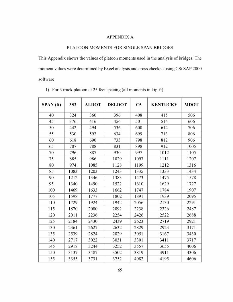
69

APPENDIX A

PLATOON MOMENTS FOR SINGLE SPAN BRIDGES

This Appendix shows the values of platoon moments used in the analysis of bridges. The

moment values were determined by Excel analysis and cross checked using CSi SAP 2000

software

1) For 3 truck platoon at 25 feet spacing (all moments in kip-ft)

SPAN (ft) 3S2 ALDOT DELDOT C5 KENTUCKY MDOT

40 324 360 396 408 415 506 45 376 416 456 501 514 606 50 442 494 536 600 614 706 55 530 592 634 699 713 806 60 618 690 733 798 812 906 65 707 788 831 898 912 1005 70 796 887 930 997 1012 1105 75 885 986 1029 1097 1111 1207 80 974 1085 1128 1199 1212 1316 85 1083 1203 1243 1335 1333 1434 90 1212 1346 1383 1473 1475 1578 95 1340 1490 1522 1610 1629 1727

100 1469 1633 1662 1747 1784 1907 105 1598 1777 1802 1891 1939 2095 110 1729 1924 1942 2056 2130 2291 115 1870 2080 2092 2238 2326 2487 120 2011 2236 2254 2426 2522 2688 125 2184 2430 2439 2623 2719 2921 130 2361 2627 2632 2829 2923 3171 135 2539 2824 2829 3051 3167 3430 140 2717 3022 3031 3301 3411 3717 145 2918 3244 3252 3557 3655 4006 150 3137 3487 3502 3819 3911 4306 155 3355 3731 3752 4082 4195 4606

70

160 3587 3986 4012 4344 4493 4905 165 3818 4243 4272 4618 4793 5205 170 4049 4499 4532 4918 5092 5505 175 4280 4755 4792 5218 5392 5805 180 4511 5011 5053 5518 5692 6105 185 4776 5309 5352 5817 5992 6405 190 5046 5609 5652 6117 6292 6705 195 5315 5908 5951 6417 6592 7005 200 5585 6208 6251 6717 6892 7304 205 5854 6508 6550 7017 7192 7604 210 6124 6807 6850 7317 7492 7904 215 6393 7107 7149 7617 7791 8204 220 6663 7406 7449 7917 8091 8504 225 6932 7706 7748 8217 8391 8804 230 7202 8005 8048 8516 8691 9104 235 7472 8305 8348 8816 8991 9404 240 7741 8604 8647 9116 9291 9704 245 8011 8904 8947 9416 9591 10004 250 8281 9203 9247 9716 9891 10304 255 8550 9503 9547 10016 10190 10604 260 8820 9802 9847 10316 10490 10904 265 9090 10102 10147 10616 10790 11204 270 9360 10402 10447 10915 11090 11504 275 9630 10702 10746 11215 11390 11804 280 9900 11002 11046 11515 11690 12104 285 10170 11302 11346 11815 11990 12404 290 10440 11602 11646 12115 12290 12704 295 10710 11902 11946 12415 12589 13004 300 10979 12201 12246 12715 12889 13304 305 11249 12501 12546 13015 13189 13604 310 11519 12801 12846 13314 13489 13904 315 11789 13101 13145 13614 13789 14204 320 12059 13401 13445 13914 14089 14504 325 12329 13701 13745 14214 14389 14804 330 12599 14001 14045 14514 14689 15104 335 12869 14301 14345 14814 14989 15404 340 13139 14600 14645 15114 15288 15704

71

345 13409 14900 14945 15414 15588 16004 350 13678 15200 15245 15714 15888 16304 355 13948 15500 15545 16013 16188 16604 360 14218 15800 15844 16313 16488 16904

2) For 3 truck platoon at 50 feet spacing (all moments in kip-ft)

SPAN (ft) 3S2 ALDOT DELDOT C5 KENTUCKY MDOT

40 324 360 396 408 415 506 45 376 416 456 501 514 606 50 442 494 536 600 614 706 55 530 592 634 699 713 806 60 618 690 733 798 812 906 65 707 788 831 898 912 1005 70 796 887 930 997 1012 1105 75 885 986 1029 1097 1111 1205 80 974 1085 1128 1196 1211 1305 85 1063 1184 1228 1296 1310 1405 90 1153 1283 1327 1396 1410 1505 95 1242 1383 1427 1496 1510 1605

100 1332 1482 1526 1595 1610 1705 105 1421 1581 1625 1695 1710 1805 110 1511 1681 1725 1795 1810 1905 115 1601 1780 1825 1895 1910 2005 120 1690 1880 1924 1995 2009 2105 125 1780 1980 2024 2095 2109 2209 130 1875 2085 2126 2218 2224 2325 135 2003 2226 2265 2354 2365 2468 140 2131 2369 2404 2490 2516 2648 145 2259 2511 2542 2627 2670 2829 150 2387 2653 2681 2792 2852 3012 155 2517 2800 2819 2972 3046 3205 160 2661 2960 2986 3153 3239 3399 165 2823 3141 3169 3344 3433 3592 170 2997 3335 3353 3536 3627 3787 175 3172 3530 3542 3728 3822 3983

72

180 3348 3724 3734 3920 4017 4188 185 3525 3920 3928 4119 4212 4434 190 3701 4116 4121 4327 4433 4717 195 3877 4312 4322 4563 4676 5006 200 4054 4508 4528 4826 4925 5304 205 4271 4748 4759 5088 5195 5604 210 4494 4995 5019 5351 5492 5904 215 4725 5251 5279 5617 5791 6204 220 4956 5506 5539 5917 6091 6504 225 5187 5763 5799 6217 6391 6804 230 5418 6019 6059 6516 6691 7104 235 5672 6305 6348 6816 6991 7404 240 5941 6604 6647 7116 7291 7704 245 6211 6904 6947 7416 7591 8004 250 6481 7203 7247 7716 7891 8304 255 6750 7503 7547 8016 8190 8604 260 7020 7802 7847 8316 8490 8904 265 7290 8102 8147 8616 8790 9204 270 7560 8402 8447 8915 9090 9504 275 7830 8702 8746 9215 9390 9804 280 8100 9002 9046 9515 9690 10104 285 8370 9302 9346 9815 9990 10404 290 8640 9602 9646 10115 10290 10704 295 8910 9902 9946 10415 10589 11004 300 9179 10201 10246 10715 10889 11304 305 9449 10501 10546 11015 11189 11604 310 9719 10801 10846 11314 11489 11904 315 9989 11101 11145 11614 11789 12204 320 10259 11401 11445 11914 12089 12504 325 10529 11701 11745 12214 12389 12804 330 10799 12001 12045 12514 12689 13104 335 11069 12301 12345 12814 12989 13404 340 11339 12600 12645 13114 13288 13704 345 11609 12900 12945 13414 13588 14004 350 11878 13200 13245 13714 13888 14304 355 12148 13500 13545 14013 14188 14604 360 12418 13800 13844 14313 14488 14904

73

APPENDIX B

MOMENT RATIOS FOR MULTI-SPAN BRIDGES

This Appendix shows the moment ratio used for calculations of multi-span bridges. +VE

value corresponds to the moment ratio at midspan region and -VE corresponds to

moment value at support regions.

1) Moment ratios for 2 truck platoon at 30 feet spacing for bridges by LRFR

method

SPAN (ft) C5 3S2 DELDOT

+VE -VE +VE -VE +VE -VE

45 0.73 0.84 0.55 0.67 0.67 0.74 50 0.73 0.92 0.55 0.73 0.67 0.83 55 0.73 0.92 0.56 0.71 0.68 0.81 60 0.73 0.89 0.57 0.70 0.68 0.80 65 0.73 0.86 0.58 0.70 0.68 0.79 70 0.73 0.83 0.58 0.69 0.68 0.78 75 0.73 0.81 0.58 0.68 0.68 0.77 80 0.72 0.79 0.58 0.67 0.68 0.76 85 0.71 0.77 0.58 0.66 0.68 0.75 90 0.72 0.75 0.58 0.65 0.67 0.73 95 0.72 0.73 0.59 0.64 0.68 0.72 100 0.73 0.71 0.60 0.63 0.68 0.70 105 0.73 0.69 0.61 0.61 0.69 0.69 110 0.73 0.67 0.61 0.60 0.70 0.67 115 0.75 0.65 0.62 0.59 0.70 0.66 120 0.76 0.63 0.63 0.57 0.71 0.64 125 0.77 0.62 0.64 0.56 0.72 0.63 130 0.78 0.60 0.65 0.55 0.73 0.61 135 0.79 0.59 0.66 0.53 0.74 0.60 140 0.80 0.57 0.67 0.52 0.75 0.58 145 0.81 0.55 0.67 0.51 0.76 0.57 150 0.81 0.55 0.68 0.50 0.77 0.56 155 0.82 0.55 0.69 0.48 0.78 0.54

74

160 0.82 0.56 0.70 0.48 0.78 0.53 165 0.82 0.56 0.70 0.48 0.78 0.54 170 0.83 0.57 0.70 0.49 0.79 0.54 175 0.83 0.57 0.71 0.49 0.79 0.55

1) Moment ratios for 2 truck platoon at 40 feet spacing for bridges by LFR method

SPAN (ft) C5 3S2 DELDOT

+VE -VE +VE -VE +VE -VE 45 0.93 0.96 0.70 0.88 0.86 0.98 50 0.95 1.10 0.71 0.89 0.87 0.99 55 0.97 1.20 0.74 0.96 0.89 1.08 60 0.98 1.31 0.76 1.01 0.91 1.15 65 0.99 1.38 0.78 1.09 0.93 1.24 70 1.01 1.41 0.80 1.14 0.94 1.29 75 1.01 1.40 0.81 1.17 0.95 1.32 80 1.01 1.39 0.82 1.17 0.96 1.32 85 1.00 1.36 0.82 1.16 0.95 1.30 90 1.00 1.32 0.82 1.14 0.95 1.28 95 0.99 1.28 0.81 1.11 0.94 1.25 100 0.98 1.23 0.81 1.08 0.93 1.21 105 0.97 1.18 0.81 1.04 0.92 1.17 110 0.97 1.14 0.80 1.01 0.92 1.13 115 0.97 1.09 0.81 0.97 0.92 1.09 120 0.97 1.04 0.82 0.94 0.93 1.05 125 0.97 1.00 0.82 0.90 0.93 1.01 130 0.98 0.96 0.82 0.87 0.93 0.97 135 0.99 0.92 0.82 0.83 0.93 0.93 140 1.00 0.88 0.83 0.80 0.94 0.90 145 1.00 0.85 0.84 0.77 0.95 0.86 150 1.01 0.81 0.85 0.74 0.96 0.83 155 1.02 0.78 0.85 0.71 0.96 0.80 160 1.02 0.75 0.86 0.68 0.97 0.77 165 1.03 0.72 0.87 0.66 0.98 0.74 170 1.03 0.69 0.87 0.63 0.98 0.71 175 1.03 0.68 0.88 0.61 0.98 0.68

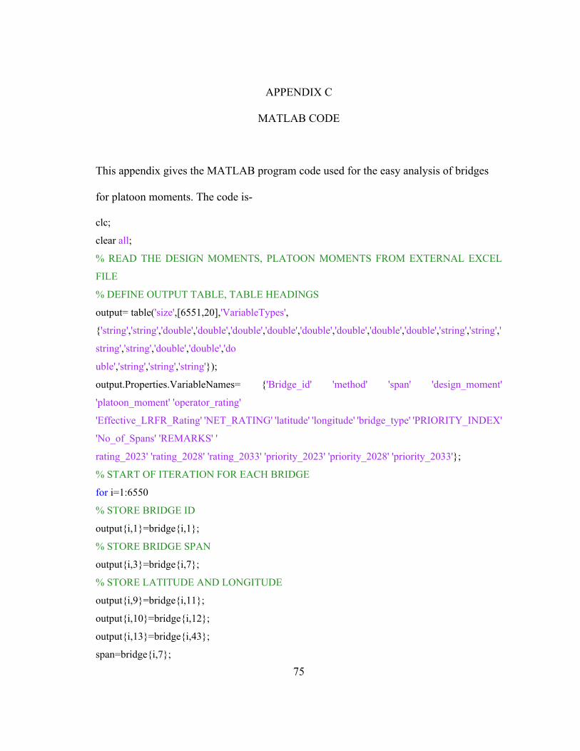
75

APPENDIX C

MATLAB CODE

This appendix gives the MATLAB program code used for the easy analysis of bridges

for platoon moments. The code is-

clc;

clear all;

% READ THE DESIGN MOMENTS, PLATOON MOMENTS FROM EXTERNAL EXCEL

FILE

% DEFINE OUTPUT TABLE, TABLE HEADINGS

output= table('size',[6551,20],'VariableTypes',

{'string','string','double','double','double','double','double','double','double','double','string','string','

string','string','double','double','do

uble','string','string','string'});

output.Properties.VariableNames= {'Bridge_id' 'method' 'span' 'design_moment'

'platoon_moment' 'operator_rating'

'Effective_LRFR_Rating' 'NET_RATING' 'latitude' 'longitude' 'bridge_type' 'PRIORITY_INDEX'

'No_of_Spans' 'REMARKS' '

rating_2023' 'rating_2028' 'rating_2033' 'priority_2023' 'priority_2028' 'priority_2033'};

% START OF ITERATION FOR EACH BRIDGE

for i=1:6550

% STORE BRIDGE ID

output{i,1}=bridge{i,1};

% STORE BRIDGE SPAN

output{i,3}=bridge{i,7};

% STORE LATITUDE AND LONGITUDE

output{i,9}=bridge{i,11};

output{i,10}=bridge{i,12};

output{i,13}=bridge{i,43};

span=bridge{i,7};

76

% CHECK FOR MULTI SPAN BRIDGES

if str2double(bridge{i,43})>1.1

if bridge{i,5}>2003

% MULTI SPAN LRFR

output{i,2}="LRFR";

for j=1:90

if str2double(multi{j,1})==span

ratio(i)= multi{j,5};

output{i,4}= str2double(multi{j,13});

output{i,5}=str2double(multi{j,13})*str2double(ratio(i));

end

end

% DETERMINE OPERATOR RATING

if str2double(bridge{i,8})>20 && str2double(bridge{i,8})<40

output{i,6}=round(1.75*1.35*output{i,4}/1.35/output{i,5},2);

else

output{i,6}=round(1.75*1.10*output{i,4}/1.35/output{i,5},2);

end

output{i,7}=round(output{i,6},2);

end

% MULTISPAN LFR

if bridge{i,5}<2004

output{i,2}="LFR";

if span <176

% LFR MULTISPAN SPAN TRIM

for j=1:85

if str2double(multi{j,1})==span

ratio(i)= multi{j,10};

output{i,4}= str2double(multi{j,17});

output{i,5}=str2double(multi{j,17})*str2double(ratio(i));

end

end

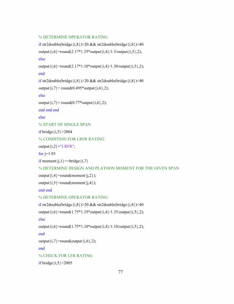
77

% DETERMINE OPERATOR RATING

if str2double(bridge{i,8})>20 && str2double(bridge{i,8})<40

output{i,6}=round(2.17*1.35*output{i,4}/1.3/output{i,5},2);

else

output{i,6}=round(2.17*1.10*output{i,4}/1.30/output{i,5},2);

end

if str2double(bridge{i,8})>20 && str2double(bridge{i,8})<40

output{i,7}= round(0.495*output{i,6},2);

else

output{i,7}= round(0.77*output{i,6},2);

end end end

else

% START OF SINGLE SPAN

if bridge{i,5}>2004

% CONDITION FOR LRFR RATING

output{i,2}="LRFR";

for j=1:93

if moment{j,1}==bridge{i,7}

% DETERMINE DESIGN AND PLATOON MOMENT FOR THE GIVEN SPAN

output{i,4}=round(moment{j,2});

output{i,5}=round(moment{j,4});

end end

% DETERMINE OPERATOR RATING

if str2double(bridge{i,8})>20 && str2double(bridge{i,8})<40

output{i,6}=round(1.75*1.35*output{i,4}/1.35/output{i,5},2);

else

output{i,6}=round(1.75*1.10*output{i,4}/1.10/output{i,5},2);

end

output{i,7}=round(output{i,6},2);

end

% CHECK FOR LFR RATING

if bridge{i,5}<2005

78

output{i,2}="LFR";

for j=1:93

if moment{j,1}==bridge{i,7}

output{i,4}=round(moment{j,3});

output{i,5}=round(moment{j,4});

end

end

if str2double(bridge{i,8})>20 && str2double(bridge{i,8})<40

output{i,6}=round(2.17*1.35*output{i,4}/1.3/output{i,5},2);

output{i,7}=round(0.495*output{i,6},2);

else

output{i,6}=round(2.17*1.1*output{i,4}/1.3/output{i,5},2);

output{i,7}=round(0.77*output{i,6},2);

end end

% CHECK FOR ASR RATING

if bridge{i,5}<1974

output{i,2}="ASR";

for j=1:93

if moment{j,1}==bridge{i,7};

output{i,4}=round(moment{j,3});

output{i,5}=round(moment{j,4});

end end

% DETERMINING CAPACITY OF THE SECTION

if str2double(bridge{i,8})>20 && str2double(bridge{i,8})<30

dead= (0.6967-0.007620*span+0.0002554*span*span)*0.8*output{i,4};

capacity= dead+0.5*1.35*output{i,4}*(1+(50/(span+125)));

elseif str2double(bridge{i,8})>=30 && str2double(bridge{i,8})<40

dead=(-0.05*span*span+17.476*span+140)*span*span*0.0001302 ;

capacity = dead+0.5*1.35*output{i,4}*(1+(50/(span+125)));

else

dead=0.0132*1.25*span*output{i,4};

capacity = dead+0.5*1.1*output{i,4}*(1+(50/(span+125)));

79

end

% DETERMINING OPERATOR RATING

if str2double(bridge{i,8})>20 && str2double(bridge{i,8})<40

output{i,6}=round(((0.75/0.55)*capacity-dead)*2/output{i,5}/(1+(50/(span+125))),2);

output{i,7}=round(0.470*output{i,6},2);

else

output{i,6}=round(((0.75/0.55)*capacity-dead)*2/output{i,5}/(1+(50/(span+125))),2);

output{i,7}=round(0.881*output{i,6},2);

end end end

if str2double(bridge{i,10})>7

output{i,8}=round(output{i,7},2);

end

if str2double(bridge{i,10})==7

output{i,8}=round(0.85*output{i,7},2);

end

if str2double(bridge{i,10})==6

output{i,8}=round(0.75*output{i,7},2);

end

if str2double(bridge{i,10})==5

output{i,8}=round(0.6*output{i,7},2);

end

if str2double(bridge{i,10})<5

output{i,8}=round(0.5*output{i,7},2);

end

% DETERMINE PRIORITY INDEX

if output{i,8}<=0.7

output{i,12}= '5';

elseif output{i,8}<=0.80&& output{i,8}>0.70

output{i,12}= '4';

elseif output{i,8}<=0.90&& output{i,8}>0.80

output{i,12}= '3';

elseif output{i,8}<=1.00&& output{i,8}>0.9

80

output{i,12}= '2';

else output{i,8}>1.0

output{i,12}= '1';

end

% DETERMINE TYPE OF BRIDGE

if str2double(bridge{i,8})>20 && str2double(bridge{i,8})<30

output{i,11}="concrete bridge";

elseif str2double(bridge{i,8})>30 && str2double(bridge{i,8})<35

output{i,11}= "prestress concrete girder";

elseif str2double(bridge{i,8})>34 && str2double(bridge{i,8})<40

output{i,11}= "prestress concrete special";

output{i,15}= 0; output{i,16}= 0;output{i,17}= 0;

output{i,20}= '0';output{i,18}= '0';output{i,19}= '0';

output{i,12}= 0;

output{i,12}= 0;

output{i,14}="Not Applicable";

elseif str2double(bridge{i,8})==30

output{i,11}= "prestress concrete segmental";

output{i,15}= 0; output{i,16}= 0;output{i,17}= 0;

output{i,20}= '0';output{i,18}= '0';output{i,19}= '0';

output{i,8}= 0;

output{i,12}= 0;

output{i,14}="Not Applicable";

elseif str2double(bridge{i,8})>40

output{i,11}= "special bridge";

output{i,15}= 0; output{i,16}= 0;output{i,17}= 0;

output{i,20}= '0';output{i,18}= '0';output{i,19}= '0';

output{i,8}= 0;

output{i,12}= 0;

output{i,14}="Not Applicable";

elseif str2double(bridge{i,8})<9

output{i,11}= "steel weathered girder";

81

elseif str2double(bridge{i,8})>10 && str2double(bridge{i,8})<19

output{i,11}= "steel girder";

else

output{i,11}= "steel special";

output{i,15}= 0; output{i,16}= 0;output{i,17}= 0;

output{i,20}= '0';output{i,18}= '0';output{i,19}= '0';

output{i,12}= 0;

output{i,8}= 0;

output{i,14}="Not Applicable";

end

if str2double(bridge{i,43})>1.1

if span >176

output{i,11}= "Multi Span Long";

output{i,15}= 1; output{i,16}= 1;output{i,17}= 1;

output{i,20}= '1';output{i,18}= '1';output{i,19}= '1';

output{i,8}= 1;

output{i,12}= 1;

output{i,14}="Special Category";

end end

end

% PRINT OUTPUT TABLE TO EXCEL- update the file directory

writetable (output,'C:\MATLAB\output.csv');

82

APPENDIX D

LRFR LOAD RATING OF STANDARD STEEL GIRDERS

SPAN  Section Weight (lbs) 

DL Moment Steel 

DL Moment Slab 

Total DL 

Capacity (kipft) 

LLF LL 

Moment IR  OR 

60  W21 x 1 66  38800  73  377  450  2653  0.73  1093  1.11  1.44 

60  W24 x 1 31  33750  63  377  440  2451  0.73  1093  1.01  1.31 

60  W27 x 1 46  35530  67  377  444  2951  0.73  1093  1.27  1.65 

60  W30 x 1 73  44430  83  377  460  3691  0.73  1093  1.66  2.15 

60  W33 x 11 8  33560  63  377  440  2989  0.73  1093  1.30  1.68 

60  W36 x 1 35  35850  67  377  444  3562  0.73  1093  1.60  2.08 

60  W40 x 1 49  38250  72  377  449  4090  0.73  1093  1.88  2.44 

     

65  W24 x 1 62  47010  95  443  538  2904  0.72  1262  1.04  1.35 

65  W27 x 1 46  42910  87  443  530  2951  0.72  1262  1.07  1.38 

65  W30 x 1 73  50000  102  443  544  3691  0.72  1262  1.41  1.82 

65  W33 x 1 30  39640  81  443  523  3229  0.72  1262  1.20  1.56 

65  W36 x 1 35  40980  83  443  526  3562  0.72  1262  1.36  1.76 

65  W40 x 1 49  44760  91  443  534  4090  0.72  1262  1.60  2.08 

 

70  W24 x 207  62830  137  513  651  3439  0.71  1376  1.14  1.47 

70  W27 x 1 78  54800  120  513  633  3460  0.71  1376  1.15  1.50 

70  W30 x 1 73  53510  117  513  630  3691  0.71  1376  1.26  1.63 

70  W33 x 1 41  45440  99  513  613  3447  0.71  1376  1.16  1.50 

70  W36 x 1 35  43720  96  513  609  3562  0.71  1376  1.21  1.57 

70  W40 x 1 49  47790  105  513  618  4090  0.71  1376  1.44  1.87 

 

75  W27 x 21 7  70050  164  589  753  4094  0.70  1524  1.25  1.62 

75  W30 x 1 91  62390  146  589  736  4022  0.70  1524  1.23  1.59 

75  W33 x 1 69  56580  133  589  722  4005  0.70  1524  1.23  1.59 

75  W36 x 1 60  53940  126  589  716  4086  0.70  1524  1.26  1.64 

75  W40 x 1 49  50820  119  589  708  4022  0.70  1524  1.24  1.61 

 

80  W27 x 235  81170  203  670  873  4420  0.69  1676  1.21  1.57 

80  W30 x 1 91  67190  168  670  838  4022  0.69  1676  1.08  1.40 

80  W33 x 201  71440  179  670  849  4568  0.69  1676  1.28  1.65 

80  W36 x 1 70  61610  154  670  825  4315  0.69  1676  1.19  1.55 

80  W40 x 1 67  60790  152  670  822  4539  0.69  1676  1.28  1.66 

 

83

85  W30 x 235  85870  228  757  985  4828  0.69  1831  1.21  1.57 

85  W33 x 221  82270  219  757  975  4986  0.69  1831  1.27  1.64 

85  W36 x 1 94  73170  194  757  951  4837  0.69  1831  1.23  1.59 

85  W40 x 1 83  69580  185  757  942  4886  0.69  1831  1.25  1.62 

 

90  W30 x 261  99940  281  849  1130  5313  0.68  1991  1.22  1.58 

90  W33 x 241  93910  264  849  1113  5230  0.68  1991  1.20  1.55 

90  W36 x 231  90360  254  849  1103  5555  0.68  1991  1.30  1.69 

90  W40 x 1 99  79020  222  849  1071  5168  0.68  1991  1.19  1.55 

 

95  W33 x 291  117630  349  945  1295  5795  0.67  2155  1.21  1.57 

95  W36 x 231  94950  282  945  1227  5555  0.67  2155  1.17  1.51 

95  W40 x 21 5  69043  205  945  1150  5562  0.67  2155  1.20  1.56 

 

100  W36 x 247  105980  331  1048  1379  5884  0.67  2323  1.13  1.46 

100  W40 x 249  107000  334  1048  1382  6366  0.67  2323  1.26  1.64 

105  W36 x 282  126780  416  1155  1571  6667  0.66  2495  1.20  1.55 

105  W40 x 277  124950  410  1155  1565  7008  0.66  2495  1.29  1.67 

110  W40 x 277  130540  449  1268  1716  7008  0.66  2670  1.17  1.51 

115  W40 x 297  145290  522  1385  1908  7456  0.65  2850  1.15  1.49 

120  W40 x 324  164190  616  1509  2124  8130  0.65  3034  1.17  1.52 

  Mean  1.22 

St. Dev.  0.05 

80 percentile  1.15 

84

APPENDIX E

LRFR LOAD RATING ANALYSIS PRESTRESS GIRDERS

Spacing  span girder LL factor DL mom LL mom strands  dia  e  d  D  fc  beta  Aps  fps  Mn  IR  OR 

6.67  65  Tx46  0.65  794.3  1232  12  0.6  17.6  52.0  43.5  5.0  0.8  3.4  254.8  3653  1.37  1.78 

6.67  70  Tx46  0.64  921.2  1376  14  0.6  17.6  52.0  43.5  5.0  0.8  4.0  252.4  4205  1.43  1.86 

6.67  75  Tx46  0.62  1057.5  1524  16  0.6  17.4  51.8  43.3  5.0  0.8  4.5  250.0  4718  1.48  1.92 

6.67  80  Tx46  0.61  1203.3  1675  18  0.6  17.2  51.6  43.1  5.4  0.8  5.1  248.6  5253  1.51  1.96 

6.67  85  Tx46 0.6  1358.4  1831  24  0.6  13.6  48.0  39.5  5.0  0.8  6.8  239.0  6160  1.68  2.18 

6.67  90  Tx46  0.59  1522.9  1991  26  0.6  13.8  48.2  39.7  5.2  0.8  7.4  237.6  6644  1.66  2.16 

6.67  95  Tx46  0.59  1696.8  2154  28  0.6  13.9  48.3  39.8  6.0  0.8  7.9  238.2  7218  1.65  2.14 

6.67  100  Tx46  0.58  1880.1  2322  32  0.6  14.0  48.4  39.9  6.4  0.7  9.1  235.4  8146  1.77  2.30 

 

6.67  90  TX54  0.61  1584.6  1991  18  0.6  20.6  59.6  51.1  9.4  0.6  5.1  255.3  6338  1.47  1.91 

6.67  95  TX54  0.6  1765.6  2154  20  0.6  20.4  59.4  50.9  10.4  0.5  5.7  253.9  6986  1.51  1.96 

6.67  100  TX54  0.6  1956.3  2322  28  0.6  16.7  55.7  47.2  11.4  0.5  7.9  246.5  8854  1.90  2.46 

6.67  105  TX54  0.59  2156.9  2494  30  0.6  16.9  55.9  47.4  12.4  0.4  8.5  244.5  9439  1.89  2.45 

6.67  110  TX54  0.58  2367.2  2670  32  0.6  16.9  55.9  47.4  13.4  0.4  9.1  241.8  9965  1.86  2.41 

ACTUAL BRIDGE STUDY

BRIDGE ID  2184031407232 

6.96  100  TX54  0.71  1987.7  2322  42  0.5  19.0  56.5  48.0  5.0  0.8  8.3  238.1  8758  1.57  2.04 

6.96  100  TX54  0.71  1987.7  2322  44  0.5  18.8  56.3  47.8  5.0  0.8  8.6  236.7  9069  1.65  2.14 

6.96  100  TX54  0.71  1987.7  2322  50  0.5  18.4  55.8  47.3  5.1  0.8  9.8  233.0  9998  1.89  2.45 

8.13  100  TX54  0.691  2135.9  2322  48  0.5  18.5  57.1  48.6  5.1  0.8  9.4  234.9  9941  1.88  2.43 

8.33  100  TX54  0.68  2162.5  2322  48  0.5  18.5  57.3  48.8  5.0  0.8  9.4  234.6  9955  1.90  2.46 

85

APPENDIX F

EXAMPLE LOAD RATING ANALYSIS CALCULATION

Example 1- LRFR Prestress Bridge

INPUTS  Units   

Bridge ID  10920004703424 

Max Span Length  100  ft   

Year Built/Rebuilt  2005 

Method of Design  LRFR 

Type of Bridge  Prestress Concrete 

Span Type  Simply Supported 

Truck Type  C5 

Spacing  30  ft   

No: of Trucks  3 

Structural Evaluation Rating  7 

CALCULATION  Note: 

Assumed I.R. by Bridge Type  1.35  From Table 2 

Υ IR  1.75  From AASHTO 

Υ OR  1.35  From AASHTO 

Design Live Load Moment (L Design)  2322  kip‐ft  SAP 2000 Analysis 

Design Capacity Minus DL Moment (C‐DL) 

5486  kip‐ft  L Design*I.R.*Υ IR 

Platoon Moment (L Platoon)  1675  kip‐ft  SAP 2000 Analysis 

Operator Rating for Platoon (OR)  2.43  (C‐DL)/ (L Platoon *Υ OR) 

LRFR Conversion Factor (C1)  1  From Table 3 

Evaluation Rating Conversion Factor (C2) 

0.85    From Table 5 

Effective Operator Rating (E.O.R.)  2.07  OR*C1*C2 

Priority Index  1  By Table 6 

86

Example 2- LFR Steel Bridge

INPUTS  Units   Bridge ID  22200000813416  Max Span Length  155  ft   Year Built/Rebuilt  2001  Method of Design  LFR  Type of Bridge  Steel Girder  Span Type  Simply Supported  Truck Type  C5  Spacing  30  ft   No:of Trucks  3  Structural Evaluation Rating  7 

CALCULATION  Units  Note: 

Assumed I.R. by Bridge Type  1.1  From Table 2 

Υ IR  2.17  From AASHTO 

Υ OR  1.3  From AASHTO 

Design Live Load Moment (L Design)  2618  kip‐ft  SAP 2000 Analysis Design Capacity Minus DL Moment (C‐DL)  6249  kip‐ft  L Design*I.R.*Υ IR 

Platoon Moment (L Platoon)  3756  kip‐ft  SAP 2000 Analysis 

Operator Rating for Platoon (OR)  1.28  (C‐DL)/(L Platoon *Υ OR) 

LRFR Conversion Factor (C1)  0.77  From Table 3 Evaluation Rating Conversion Factor (C2) 

0.85    From Table 5 

Effective Operator Rating  (E.O.R.)  0.84  OR*C1*C2 

Priority Index  3  By Table 6 

87

APPENDIX G

EXAMPLE OUTPUT OBTAINED BY VBA ANALYSIS

This Appendix gives output obtained for highway district 2 for 3 truck C5 platoon at 30

ft spacing

Bridge ID Highway District 

SpanYear Built/ Rebuilt 

Operator Rating 

Priority Rating 

Priority Index 

21270001403495  2  90  2008  2.49  2.12  1 

21820031403132  2  65  1970  2.21  0.88  3 

21820031403134  2  95  1970  2.33  0.94  2 

21820031403135  2  95  1970  2.33  0.94  2 

21840000803274  2  100  1978  2.05  0.86  3 

21840000803276  2  75  1978  2.21  0.93  2 

21840031401083  2  145  2008  1.7  1.44  1 

21840031407064  2  50  1969  2.2  0.77  4 

21840031407232  2  100  2017  2.43  2.43  1 

22200000812357  2  125  1991  1.81  0.77  4 

22200000812464  2  115  2013  2.38  2.02  1 

22200000813092  2  75  1988  1.29  0.84  3 

22200000813093  2  75  1988  1.29  0.84  3 

22200000813100  2  75  1963  1.29  0.59  5 

22200000813104  2  65  1963  1.25  0.72  4 

22200000813126  2  90  1963  1.36  0.79  4 

22200000813343  2  60  1988  2.28  0.85  3 

22200000813416  2  155  2001  1.28  0.84  3 

22200000813419  2  120  2002  1.87  0.79  4 

22200000813421  2  180  1990  0  1  1 

22200000813429  2  125  1990  1.81  0.68  5 

22200000813430  2  125  1990  1.81  0.68  5 

22200000814201  2  75  1973  2.26  0.8  4 

22200000814204  2  140  1973  1.52  0.99  2 

22200000814205  2  140  1973  1.52  0.99  2 

22200000814261  2  75  1977  2.21  0.93  2 

22200000814488  2  110  2014  2.4  2.04  1 

22200000814490  2  95  2014  2.45  2.08  1 

22200000814499  2  130  2013  2.26  1.92  1 

22200000814514  2  190  2014  1.85  1.57  1 

88

22200000814521  2  130  2014  2.26  1.36  1 

22200000814525  2  100  2014  2.43  2.07  1 

22200000815227  2  110  1976  1.97  0.74  4 

22200000815228  2  110  1976  1.97  0.83  3 

22200000815294  2  120  1982  1.87  0.7  5 

22200000815300  2  130  1982  1.76  0.65  5 

22200000816251  2  120  1995  1.87  0.56  5 

22200001415331  2  80  1970  2.29  0.81  3 

22200001415383  2  75  1976  2.21  0.82  3 

22200001416189  2  55  1961  1.62  0.48  5 

22200001416391  2  85  1981  2.18  0.92  2 

22200001416408  2  70  1988  2.23  0.94  2 

22200001416457  2  120  2001  1.87  0.79  4 

22200001416459  2  95  2001  2.1  0.88  3 

22200001416478  2  125  2000  1.48  0.97  2 

22200001416539  2  130  2014  2.26  1.92  1 

22200001416541  2  95  2014  2.45  2.45  1 

22200001416573  2  90  2016  2.49  2.49  1 

22200001416593  2  235  2016  1.74  1.74  1 

22200001416601  2  120  2016  2.33  2.33  1 

22200001416619  2  145  2016  2.16  2.16  1 

22200001416628  2  270  2018  Inf  1  1 

22200008112077  2  60  1990  2.28  0.85  3 

22200008112222  2  80  1997  2.2  0.93  2 

22200008112223  2  65  1997  2.25  0.94  2 

22200009402067  2  125  1974  1.81  0.68  5 

22200009402069  2  80  1974  2.2  0.93  2 

22200035303433  2  140  2012  2.19  1.86  1 

22200036401411  2  120  2001  1.87  0.79  4 

22200036401674  2  100  2014  2.43  2.07  1 

22200036401688  2  115  2014  2.38  2.38  1 

22200050402470  2  75  2014  2.43  2.43  1 

22200050402483  2  115  2014  2.38  2.38  1 

22200106801117  2  60  1989  1.55  0.58  5 

22200106801126  2  65  1965  2.21  0.88  3 

22200106801138  2  85  1975  2.18  0.92  2 

22200106801289  2  125  2000  1.81  0.77  4 

22200106801293  2  150  2000  1.3  0.85  3 

22200106801483  2  120  2000  1.87  0.79  4 

22200106801563  2  100  2017  2.43  2.43  1 

89

22200106802037  2  70  1957  1.54  0.46  5 

22200106802047  2  95  1957  1.38  0.64  5 

22200106802058  2  105  1957  1.37  0.79  4 

22200106802271  2  90  1957  2.28  1.51  1 

22200106802284  2  50  1997  2.36  0.99  2 

22200106802286  2  110  1997  1.97  0.83  3 

22200106802288  2  90  1997  2.16  0.91  2 

22200106802302  2  90  2000  2.16  0.91  2 

22200106802332  2  85  1983  2.18  0.81  3 

22200106802376  2  200  1991  0  1  1 

22200106802551  2  120  2017  2.33  2.33  1 

22200106802554  2  120  2017  2.33  2.33  1 

22200106802557  2  70  2017  2.42  2.42  1 

22200106802567  2  215  2017  Inf  1  1 

22200106802568  2  245  2017  Inf  1  1 

22200226602092  2  70  1992  2.23  0.94  2 

22200237405232  2  100  1973  2.32  0.82  3 

22200237405275  2  65  1974  2.25  0.94  2 

22200237405279  2  110  2010  2.4  1.8  1 

22200237405289  2  85  1975  2.18  0.81  3 

22490001306059  2  55  1981  2.31  0.97  2 

22490001306068  2  85  1977  2.18  0.92  2 

22490001308053  2  85  1972  2.32  0.82  3 

21270001403198  2  75  1988  1.29  0.74  4 

21270001403231  2  50  1965  2.2  0.77  4 

21270001404276  2  65  1966  2.21  0.88  3 

21270001422293  2  65  1966  2.21  0.62  5 

21270001422294  2  65  1966  2.21  0.78  4 

21270001422297  2  50  1966  2.2  0.77  4 

21820031402096  2  85  1971  2.32  0.55  5 

21820031402099  2  45  1971  2.23  0.79  4 

21820031403145  2  75  1970  2.26  0.9  3 

21840000803273  2  100  1978  2.05  0.86  3 

21840000803315  2  190  1986  0  1  1 

21840031401074  2  80  1970  2.29  0.65  5 

21840031401076  2  75  1970  2.26  0.9  3 

21840031401080  2  60  1970  2.2  0.77  4 

21840031401081  2  80  1970  2.29  0.65  5 

21840031407045  2  90  1968  1.36  0.63  5 

21840031407047  2  75  1968  2.26  0.8  4 

90

22200000812385  2  65  1995  2.25  0.94  2 

22200000812386  2  100  1995  2.05  0.76  4 

22200000812392  2  70  1995  2.23  0.94  2 

22200000812465  2  115  2014  2.38  2.02  1 

22200000813099  2  65  1963  1.25  0.58  5 

22200000813120  2  60  1963  2.2  0.77  4 

22200000813131  2  50  1963  2.2  0.77  4 

22200000813136  2  80  1963  1.33  0.61  5 

22200000813264  2  50  1988  1.43  0.83  3 

22200000813354  2  85  1990  2.18  0.92  2 

22200000813380  2  80  1991  2.2  0.82  3 

22200000813436  2  105  1989  2.01  0.74  4 

22200000813529  2  145  2018  2.16  2.16  1 

22200000813530  2  140  2018  2.19  2.19  1 

22200000814203  2  140  1973  1.52  0.99  2 

22200000814207  2  70  1973  2.23  0.89  3 

22200000814209  2  75  1973  2.26  0.8  4 

22200000814260  2  75  1977  2.21  0.93  2 

22200000814398  2  105  1997  2.01  0.84  3 

22200000814400  2  105  2014  2.41  2.05  1 

22200000814491  2  95  2014  2.45  2.08  1 

22200000814497  2  125  2012  2.3  2.3  1 

22200000814506  2  120  2013  2.33  2.33  1 

22200000815219  2  120  1975  1.87  0.7  5 

22200000815303  2  115  1982  1.93  0.72  4 

22200000816328  2  100  1986  2.05  0.76  4 

22200000816469  2  125  2013  2.3  1.95  1 

22200000816470  2  100  2011  2.43  2.07  1 

22200000816471  2  75  2011  2.43  2.43  1 

22200000816472  2  240  2014  Inf  1  1 

22200001415384  2  95  1976  2.1  0.88  3 

22200001415385  2  80  1996  2.2  0.93  2 

22200001416192  2  85  1961  1.35  0.78  4 

22200001416453  2  90  1999  2.16  0.91  2 

22200001416534  2  85  2012  2.47  2.1  1 

22200001416546  2  215  2014  Inf  1  1 

22200001416548  2  220  2014  Inf  1  1 

22200001416561  2  125  2016  2.3  1.95  1 

22200001416564  2  140  2016  2.19  2.19  1 

22200001416577  2  110  2016  2.4  2.4  1 

91

22200001416579  2  135  2016  2.23  2.23  1 

22200001416589  2  120  2016  2.33  2.33  1 

22200001416617  2  100  2016  2.43  2.43  1 

22200008112082  2  65  1967  2.21  0.78  4 

22200008112084  2  65  1967  2.21  0.78  4 

22200036303415  2  130  2018  2.26  2.26  1 

22200036401655  2  135  2014  2.23  1.9  1 

22200036401670  2  115  2014  2.38  2.38  1 

22200036401684  2  115  2014  2.38  2.38  1 

22200106801167  2  95  1988  1.38  0.8  4 

22200106801276  2  80  1989  2.2  0.93  2 

22200106801291  2  165  2000  1.25  0.72  4 

22200106801446  2  180  2000  1.22  0.71  4 

22200106801484  2  115  2001  1.93  0.82  3 

22200106801509  2  125  2014  2.3  1.95  1 

22200106801511  2  250  2013  Inf  1  1 

22200106801520  2  230  2013  Inf  1  1 

22200106801564  2  100  2017  2.43  2.43  1 

22200106802039  2  70  1957  1.54  0.57  5 

22200106802149  2  70  1961  2.23  0.79  4 

22200106802198  2  60  1997  2.28  0.96  2 

22200106802283  2  50  1997  2.36  0.99  2 

22200106802285  2  110  1997  1.97  0.83  3 

22200106802377  2  150  1991  1.6  0.92  2 

22200106802378  2  200  1991  0  1  1 

22200106802382  2  65  1991  2.25  0.83  3 

22200106802488  2  120  2010  2.33  2.33  1 

22200106802489  2  120  2011  2.33  1.98  1 

22200106802553  2  190  2017  Inf  1  1 

22200106802556  2  215  2017  Inf  1  1 

22200133001018  2  110  2004  1.97  0.83  3 

22200226602088  2  75  1992  2.21  0.93  2 

22200226602089  2  75  1992  2.21  0.93  2 

22200237405196  2  115  1972  2.32  0.82  3 

22200237405269  2  70  1974  2.23  0.94  2 

22200237405287  2  115  1975  1.93  0.72  4 

22200237405496  2  110  2005  2.4  2.4  1 

022200S53350001  2  80  1994  2.2  0.93  2 

22490001307064  2  60  1981  2.28  0.85  3 

22490001307086  2  95  1986  2.1  0.88  3 

92

22490001308091  2  80  1996  2.2  0.93  2 

22490001308092  2  80  1996  2.2  0.93  2 

21270001403196  2  70  1963  1.26  0.73  4 

21270001404057  2  60  1939  2.09  1.1  1 

21270001404059  2  60  1987  1.86  0.86  3 

21270001404202  2  55  1963  1.62  0.6  5 

21270001404268  2  65  1966  2.21  0.52  5 

21270001404280  2  65  1966  2.21  0.78  4 

21820031402102  2  75  1971  2.26  0.8  4 

21840000803280  2  95  2018  2.45  2.08  1 

21840000803316  2  140  1986  1.52  0.7  5 

21840031401075  2  75  1970  2.26  0.8  4 

21840031407046  2  75  1968  2.26  0.8  4 

21840031407048  2  50  1968  2.2  0.88  3 

21840031407056  2  65  1969  2.21  0.78  4 

21840031407067  2  65  1969  2.21  0.52  5 

21840031407224  2  90  2012  2.49  2.49  1 

21840031407228  2  120  2014  2.33  2.33  1 

22200000812358  2  110  1991  1.97  0.83  3 

22200000813117  2  75  1963  1.29  0.59  5 

22200000813122  2  65  1963  2.21  0.78  4 

22200000813129  2  65  1963  2.21  0.78  4 

22200000813134  2  70  1963  2.23  0.79  4 

22200000813313  2  80  1963  1.33  0.77  4 

22200000813346  2  135  1991  1.49  0.86  3 

22200000813424  2  210  1990  0  1  1 

22200000814206  2  140  1973  1.52  0.99  2 

22200000814285  2  125  1976  1.81  0.68  5 

22200000814486  2  100  2013  2.43  2.07  1 

22200000814516  2  185  2014  1.87  1.59  1 

22200000815296  2  95  1982  2.1  0.78  4 

22200000816319  2  120  1986  1.87  0.7  5 

22200000816321  2  180  1986  0  1  1 

22200000816322  2  180  1986  0  1  1 

22200000816327  2  215  1986  0  1  1 

22200000816475  2  125  2014  2.3  1.95  1 

22200000816478  2  125  2014  2.3  1.72  1 

22200001402355  2  80  1992  2.2  0.93  2 

22200001402356  2  115  1976  1.93  0.82  3 

22200001415330  2  95  1970  1.38  0.8  4 

93

22200001415336  2  95  1970  1.38  0.64  5 

22200001416190  2  60  1961  1.55  0.46  5 

22200001416392  2  75  1981  2.21  0.82  3 

22200001416397  2  85  1982  2.18  0.92  2 

22200001416417  2  170  1988  1.59  1.04  1 

22200001416438  2  80  1990  2.2  0.93  2 

22200001416452  2  275  2001  0  1  1 

22200001416532  2  125  2013  2.3  1.95  1 

22200001416538  2  130  2014  2.26  1.92  1 

22200001416580  2  130  2016  2.26  2.26  1 

22200001416596  2  120  2016  2.33  2.33  1 

22200001416616  2  100  2016  2.43  2.43  1 

22200001416620  2  145  2016  2.16  2.16  1 

22200008112076  2  60  1967  2.2  0.77  4 

22200008112078  2  65  1967  2.21  0.78  4 

22200008112168  2  105  1991  2.01  0.74  4 

22200036401415  2  235  2001  0  1  1 

22200036401686  2  115  2014  2.38  2.38  1 

22200106801120  2  65  1965  2.21  0.78  4 

22200106801130  2  60  1965  2.2  0.62  5 

22200106801160  2  185  2011  Inf  1  1 

22200106801218  2  120  1975  1.87  0.79  4 

22200106801274  2  95  1989  1.38  0.9  3 

22200106801278  2  120  1988  1.87  0.7  5 

22200106801290  2  125  2000  1.81  0.68  5 

22200106801324  2  115  2003  1.93  0.82  3 

22200106801447  2  230  2000  0  1  1 

22200106801454  2  115  2001  1.93  0.72  4 

22200106801482  2  120  2000  1.87  0.7  5 

22200106801495  2  240  2016  Inf  1  1 

22200106801507  2  125  2014  2.3  1.95  1 

22200106801521  2  230  2013  Inf  1  1 

22200106802062  2  65  1993  1.25  0.82  3 

22200106802140  2  80  1976  2.2  0.82  3 

22200106802180  2  80  1976  2.2  0.82  3 

22200106802200  2  60  1997  2.28  0.96  2 

22200106802370  2  85  1997  2.18  0.92  2 

22200106802371  2  115  1997  1.93  0.82  3 

22200106802486  2  95  2010  2.45  2.45  1 

22200106802487  2  120  2010  2.33  2.33  1 

94

22200106802548  2  130  2017  2.26  2.26  1 

22200106802555  2  120  2017  2.33  2.33  1 

22200226602059  2  110  1991  1.97  0.74  4 

22200226602101  2  70  1997  2.23  0.83  3 

22200237405270  2  70  1974  2.23  0.94  2 

22200237405293  2  190  1975  0  1  1 

22200237405297  2  70  1975  2.23  0.94  2 

22200237405442  2  110  1993  1.97  0.83  3 

22200237405443  2  110  1993  1.97  0.74  4 

22200237406424  2  85  1981  2.18  0.92  2 

022200GG0247005  2  60  2013  2.4  2.4  1 

22490001306058  2  55  1981  2.31  0.97  2 

22490001307065  2  60  1981  2.28  0.96  2 

21270001403195  2  70  1963  1.26  0.73  4 

21270001403232  2  50  1965  2.2  0.77  4 

21270001403236  2  60  1965  2.2  0.77  4 

21270001403243  2  70  1965  2.23  0.79  4 

21270001404201  2  55  1963  1.62  0.6  5 

21270025905079  2  130  2003  1.76  0.65  5 

21820031402094  2  60  1971  2.2  0.77  4 

21840031401079  2  60  1970  2.2  0.77  4 

21840031407051  2  65  2011  2.4  1.44  1 

21840031407059  2  65  1969  2.21  0.88  3 

21840031407065  2  50  1969  2.2  0.88  3 

21840031407220  2  110  1968  1.37  0.79  4 

21840031407233  2  110  2017  2.4  2.4  1 

21840106805515  2  125  2014  2.3  2.3  1 

22200000812393  2  100  1995  2.05  0.86  3 

22200000813119  2  60  1963  2.2  0.77  4 

22200000813133  2  60  1963  2.2  0.77  4 

22200000813135  2  75  1963  2.26  0.8  4 

22200000813263  2  50  1988  1.43  0.83  3 

22200000813341  2  80  1988  2.2  0.82  3 

22200000813344  2  85  1988  2.18  0.92  2 

22200000813413  2  135  2001  1.71  0.72  4 

22200000813423  2  215  1990  0  1  1 

22200000813426  2  90  1990  2.16  0.64  5 

22200000814187  2  90  1981  2.16  0.8  4 

22200000814234  2  80  1976  2.2  0.93  2 

22200000814238  2  110  1976  1.97  0.74  4 

95

22200000814240  2  120  1976  1.87  0.79  4 

22200000814242  2  80  1976  2.2  0.93  2 

22200000814262  2  105  1977  2.01  0.74  4 

22200000814442  2  115  2005  1.69  1.44  1 

22200000814443  2  115  2005  1.69  1.44  1 

22200000814501  2  115  2013  2.38  2.02  1 

22200000814504  2  110  2014  2.4  2.04  1 

22200000814505  2  110  2013  2.4  2.4  1 

22200000815211  2  105  1975  2.01  0.74  4 

22200000815225  2  85  1976  2.18  0.92  2 

22200000816243  2  195  1981  0  1  1 

22200000816246  2  95  1981  2.1  0.88  3 

22200000816306  2  90  1982  2.16  0.91  2 

22200000816312  2  95  1986  2.1  0.78  4 

22200000816325  2  95  1985  2.1  0.88  3 

22200000816329  2  110  1986  1.97  0.74  4 

22200001402439  2  115  2007  2.38  2.02  1 

22200001415338  2  85  1970  2.32  0.93  2 

22200001416339  2  65  2008  2.4  1.8  1 

22200001416480  2  120  2000  1.87  0.79  4 

22200001416545  2  220  2014  1.76  1.76  1 

22200001416562  2  140  2016  2.19  2.19  1 

22200001416563  2  145  2016  2.16  2.16  1 

22200001416565  2  120  2016  2.33  2.33  1 

22200001416590  2  115  2016  2.38  2.38  1 

22200001416594  2  230  2016  1.75  1.75  1 

22200001416599  2  145  2016  2.16  2.16  1 

22200001416600  2  145  2016  2.16  2.16  1 

22200001416604  2  65  2016  2.4  2.4  1 

22200001416621  2  145  2016  2.16  2.16  1 

22200008112079  2  65  1967  2.21  0.78  4 

22200008112081  2  65  1967  2.21  0.78  4 

22200035303434  2  140  2012  2.19  1.86  1 

22200036401414  2  175  2001  1.57  1.03  1 

22200036401668  2  90  2014  2.49  2.12  1 

22200036401675  2  120  2014  2.33  2.33  1 

22200036401683  2  100  2014  2.43  1.82  1 

22200036405654  2  100  2014  2.43  2.07  1 

22200050402469  2  75  2014  2.43  2.43  1 

22200050402488  2  250  2013  1.73  1.47  1 

96

22200106801116  2  55  1964  1.62  0.6  5 

22200106801139  2  85  1975  2.18  0.92  2 

22200106801215  2  125  1975  1.81  0.77  4 

22200106801277  2  140  1989  1.52  0.99  2 

22200106801294  2  110  2000  1.97  0.59  5 

22200106801349  2  80  1988  2.2  0.93  2 

22200106801350  2  80  1987  2.2  0.93  2 

22200106801448  2  165  2003  1.61  0.93  2 

22200106801499  2  120  2014  2.33  2.33  1 

22200106801506  2  125  2014  2.3  1.95  1 

22200106801512  2  250  2013  Inf  1  1 

22200106802107  2  145  1993  1.62  0.6  5 

22200106802145  2  80  1962  1.33  0.77  4 

22200106802163  2  100  1983  2.05  0.76  4 

22200106802173  2  90  1986  2.16  0.91  2 

22200106802197  2  60  1997  2.28  0.96  2 

22200106802267  2  75  1997  1.58  0.59  5 

22200106802307  2  115  2009  2.38  1.79  1 

22200106802348  2  110  1988  1.97  0.74  4 

22200106802485  2  95  2010  2.45  2.08  1 

22200106802552  2  255  2017  Inf  1  1 

22200106802559  2  70  2017  2.42  2.42  1 

22200106802561  2  70  2017  2.42  2.42  1 

22200106802566  2  205  2017  Inf  1  1 

22200106802569  2  215  2017  Inf  1  1 

22200106802570  2  225  2017  Inf  1  1 

22200226602073  2  75  1994  2.21  0.93  2 

22200237405276  2  70  1974  2.23  0.83  3 

22200237405281  2  110  1993  1.97  0.74  4 

22200237405495  2  110  2005  2.4  2.04  1 

22200237406422  2  75  1981  2.21  0.82  3 

22490001306061  2  70  1981  2.23  0.94  2 

22490001308069  2  95  1990  2.1  0.88  3 

20730031404117  2  80  1970  2.29  0.81  3 

21270001403193  2  60  2007  1.6  0.96  2 

21270001403194  2  80  1963  1.33  0.51  5 

21270001403197  2  80  1988  1.33  0.77  4 

21270001404272  2  65  1966  2.21  0.78  4 

21270001422295  2  65  1966  2.21  0.78  4 

21270001422298  2  50  1966  2.2  0.77  4 

97

21820031402098  2  45  1971  2.23  0.79  4 

21820031402107  2  75  1971  2.26  0.9  3 

21820031403146  2  75  1970  2.26  0.9  3 

21840031401084  2  80  1970  2.29  0.81  3 

21840031407061  2  85  1969  1.35  0.78  4 

21840031407230  2  65  2017  2.4  2.4  1 

22130025903023  2  80  2008  2.45  2.45  1 

22200000812387  2  110  1995  1.97  0.83  3 

22200000813101  2  75  1963  1.29  0.59  5 

22200000813109  2  60  1963  1.27  0.74  4 

22200000813128  2  45  1963  2.41  0.68  5 

22200000813347  2  145  1988  1.56  1.02  1 

22200000813402  2  150  1998  1.3  0.85  3 

22200000813418  2  155  2002  1.63  1.07  1 

22200000813438  2  80  1991  2.2  0.82  3 

22200000813528  2  140  2018  2.19  2.19  1 

22200000813531  2  125  2018  2.3  2.3  1 

22200000814183  2  55  1981  2.31  0.97  2 

22200000814202  2  75  1973  2.26  0.9  3 

22200000814208  2  70  1973  2.23  0.79  4 

22200000814210  2  75  1973  2.26  0.9  3 

22200000814232  2  80  1976  2.2  0.93  2 

22200000814235  2  80  1976  2.2  0.93  2 

22200000814241  2  80  1976  2.2  0.93  2 

22200000814258  2  95  1977  2.1  0.78  4 

22200000814489  2  95  2013  2.45  2.08  1 

22200000814502  2  115  2013  2.38  2.38  1 

22200000815223  2  95  1976  2.1  0.78  4 

22200000815226  2  110  1976  1.97  0.83  3 

22200000815255  2  90  1977  2.16  0.8  4 

22200000815295  2  120  1982  1.87  0.7  5 

22200000816323  2  160  1986  1.62  1.06  1 

22200000816324  2  160  1986  1.62  0.94  2 

22200000816473  2  125  2014  2.3  1.95  1 

22200000816481  2  240  2014  Inf  1  1 

22200000816482  2  125  2013  2.3  1.95  1 

22200001402496  2  100  2009  2.43  2.07  1 

22200001416150  2  80  1999  1.33  0.87  3 

22200001416390  2  100  1981  2.05  0.86  3 

22200001416431  2  105  1990  2.01  0.84  3 

98

22200001416479  2  120  2000  1.87  0.79  4 

22200001416540  2  85  2014  2.47  2.47  1 

22200001416543  2  95  2015  2.45  2.08  1 

22200001416550  2  95  2015  2.45  2.45  1 

22200001416556  2  85  2016  2.47  2.47  1 

22200001416574  2  110  2016  2.4  2.4  1 

22200001416584  2  135  2016  2.23  2.23  1 

22200001416588  2  125  2016  2.3  2.3  1 

22200001416592  2  230  2016  1.75  1.75  1 

22200001416602  2  120  2016  2.33  2.33  1 

22200001416605  2  125  2016  2.3  2.3  1 

22200001416609  2  125  2016  2.3  2.3  1 

22200001416618  2  120  2015  2.33  1.98  1 

22200008112172  2  110  1991  1.97  0.74  4 

22200008112209  2  120  2006  2.33  1.75  1 

22200009402068  2  115  1974  1.93  0.72  4 

22200036401657  2  135  2014  2.23  2.23  1 

22200036405653  2  105  2014  2.41  2.05  1 

22200106801009  2  90  1985  1.36  0.79  4 

22200106801136  2  90  1967  1.36  0.79  4 

22200106801166  2  105  1987  2.01  0.84  3 

22200106801169  2  140  1988  1.52  0.88  3 

22200106801213  2  70  1975  2.23  0.94  2 

22200106801216  2  125  1975  1.81  0.68  5 

22200106801265  2  60  1965  2.2  0.77  4 

22200106801295  2  120  2000  1.87  0.7  5 

22200106801326  2  90  2003  2.16  0.91  2 

22200106801449  2  200  2001  0  1  1 

22200106801498  2  120  2014  2.33  2.33  1 

22200106801502  2  125  2013  2.3  1.95  1 

22200106801510  2  230  2013  Inf  1  1 

22200106802036  2  80  1957  1.63  0.61  5 

22200106802287  2  90  1997  2.16  0.91  2 

22200106802301  2  90  2003  2.16  0.91  2 

22200106802360  2  95  1988  2.1  0.78  4 

22200106802372  2  75  1997  2.21  1.09  1 

22200106802375  2  220  1991  0  1  1 

22200106802415  2  125  1986  1.81  0.77  4 

22200133001017  2  125  2004  1.81  0.77  4 

22200226602060  2  115  1991  1.93  0.82  3 

99

22200226602093  2  70  1992  2.23  0.94  2 

22200237405272  2  110  1974  1.97  0.74  4 

22200237405273  2  110  1974  1.97  0.74  4 

22200237405277  2  70  1974  2.23  0.94  2 

22200237405278  2  110  2010  2.4  1.8  1 

22200237405290  2  145  1971  1.56  0.9  3 

22200237405314  2  120  1972  2.28  0.8  4 

22200237406514  2  125  2011  2.3  1.95  1 

22490001306063  2  95  1981  2.1  0.88  3 

22490001307067  2  70  1981  2.23  0.94  2 

22490001308054  2  85  1972  2.32  0.82  3 

22490001308100  2  135  1972  1.49  0.86  3 

20730031404118  2  80  1970  2.29  0.92  2 

21270001404266  2  60  1966  2.2  0.77  4 

21820031403090  2  95  1971  2.33  0.83  3 

21820031403130  2  95  1970  2.33  0.55  5 

21820031403144  2  100  1970  2.32  0.55  5 

21840000803279  2  85  1978  2.18  0.81  3 

21840031407040  2  65  2017  2.4  1.44  1 

21840031407044  2  60  1968  2.2  0.77  4 

21840031407057  2  65  1969  2.21  0.78  4 

21840031407222  2  65  2011  2.4  2.04  1 

21840031407225  2  100  2011  2.43  2.07  1 

21840106805516  2  125  2014  2.3  1.95  1 

22200000812395  2  90  1995  2.16  0.91  2 

22200000812396  2  110  1991  1.97  0.74  4 

22200000813103  2  70  1963  1.26  0.73  4 

22200000813106  2  60  1963  1.27  0.74  4 

22200000813110  2  60  1963  1.27  0.74  4 

22200000813132  2  50  1963  2.2  0.77  4 

22200000813165  2  70  1965  1.26  0.73  4 

22200000813181  2  65  1969  2.21  0.78  4 

22200000813337  2  95  1985  2.1  0.78  4 

22200000813342  2  75  1988  2.21  0.93  2 

22200000813428  2  90  1990  2.16  0.8  4 

22200000813534  2  160  2018  2.02  2.02  1 

22200000814233  2  80  1976  2.2  0.93  2 

22200000814259  2  95  1977  2.1  0.78  4 

22200000814484  2  100  2013  2.43  2.07  1 

22200000814485  2  110  2013  2.4  2.04  1 

100

22200000814496  2  125  2013  2.3  2.3  1 

22200000814498  2  110  2013  2.4  2.04  1 

22200000815254  2  90  1977  2.16  0.91  2 

22200000815257  2  125  1977  1.81  0.68  5 

22200000816244  2  140  1981  1.66  0.7  5 

22200000816286  2  110  1982  1.97  0.74  4 

22200000816467  2  125  2013  2.3  1.95  1 

22200001402340  2  70  2008  2.42  1.82  1 

22200001415333  2  85  1970  2.32  0.65  5 

22200001415386  2  85  1996  2.18  0.92  2 

22200001416191  2  55  1961  1.62  0.48  5 

22200001416412  2  135  1988  1.71  0.72  4 

22200001416427  2  105  1990  2.01  0.59  5 

22200001416443  2  100  1995  2.05  0.86  3 

22200001416464  2  70  2001  2.23  0.94  2 

22200001416466  2  120  2001  1.87  0.7  5 

22200001416544  2  175  2014  1.64  1.64  1 

22200001416547  2  180  2014  Inf  1  1 

22200001416566  2  120  2016  2.33  2.33  1 

22200001416575  2  120  2016  2.33  2.33  1 

22200001416578  2  130  2016  2.26  2.26  1 

22200001416587  2  115  2016  2.38  2.38  1 

22200001416591  2  85  2016  2.47  2.47  1 

22200001416598  2  140  2016  2.19  2.19  1 

22200001416606  2  125  2016  2.3  2.3  1 

22200001416624  2  125  2016  2.3  2.3  1 

22200008112171  2  95  1991  2.1  0.88  3 

22200008112195  2  95  1997  2.1  0.78  4 

22200008112210  2  120  2006  2.33  1.75  1 

22200009402103  2  90  1990  2.16  0.91  2 

22200017206051  2  65  1962  1.53  0.57  5 

22200035303196  2  110  2004  1.97  0.83  3 

22200036401410  2  125  2001  1.81  0.77  4 

22200036401659  2  135  2014  2.23  1.9  1 

22200050402489  2  235  2013  1.74  1.48  1 

22200106801115  2  65  1964  1.53  0.57  5 

22200106801125  2  70  1965  2.23  0.79  4 

22200106801272  2  95  1989  1.38  0.9  3 

22200106801275  2  80  1989  2.2  0.82  3 

22200106801445  2  180  2000  1.22  0.71  4 

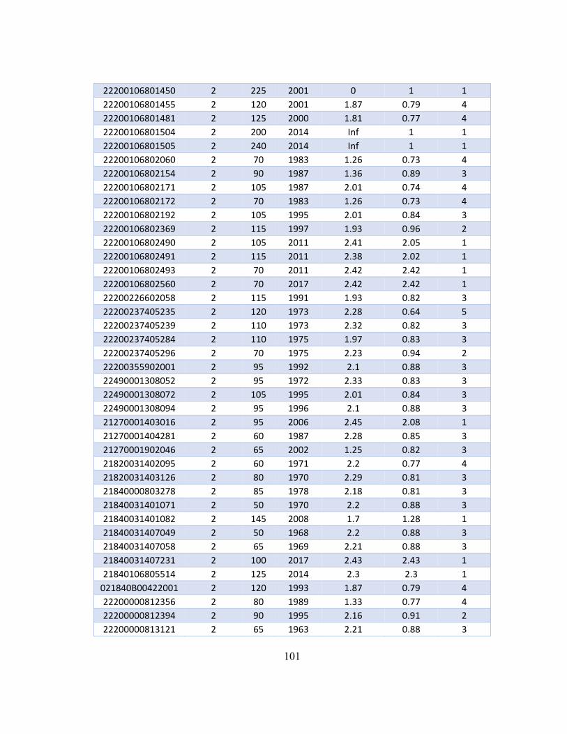
101

22200106801450  2  225  2001  0  1  1 

22200106801455  2  120  2001  1.87  0.79  4 

22200106801481  2  125  2000  1.81  0.77  4 

22200106801504  2  200  2014  Inf  1  1 

22200106801505  2  240  2014  Inf  1  1 

22200106802060  2  70  1983  1.26  0.73  4 

22200106802154  2  90  1987  1.36  0.89  3 

22200106802171  2  105  1987  2.01  0.74  4 

22200106802172  2  70  1983  1.26  0.73  4 

22200106802192  2  105  1995  2.01  0.84  3 

22200106802369  2  115  1997  1.93  0.96  2 

22200106802490  2  105  2011  2.41  2.05  1 

22200106802491  2  115  2011  2.38  2.02  1 

22200106802493  2  70  2011  2.42  2.42  1 

22200106802560  2  70  2017  2.42  2.42  1 

22200226602058  2  115  1991  1.93  0.82  3 

22200237405235  2  120  1973  2.28  0.64  5 

22200237405239  2  110  1973  2.32  0.82  3 

22200237405284  2  110  1975  1.97  0.83  3 

22200237405296  2  70  1975  2.23  0.94  2 

22200355902001  2  95  1992  2.1  0.88  3 

22490001308052  2  95  1972  2.33  0.83  3 

22490001308072  2  105  1995  2.01  0.84  3 

22490001308094  2  95  1996  2.1  0.88  3 

21270001403016  2  95  2006  2.45  2.08  1 

21270001404281  2  60  1987  2.28  0.85  3 

21270001902046  2  65  2002  1.25  0.82  3 

21820031402095  2  60  1971  2.2  0.77  4 

21820031403126  2  80  1970  2.29  0.81  3 

21840000803278  2  85  1978  2.18  0.81  3 

21840031401071  2  50  1970  2.2  0.88  3 

21840031401082  2  145  2008  1.7  1.28  1 

21840031407049  2  50  1968  2.2  0.88  3 

21840031407058  2  65  1969  2.21  0.88  3 

21840031407231  2  100  2017  2.43  2.43  1 

21840106805514  2  125  2014  2.3  2.3  1 

021840B00422001  2  120  1993  1.87  0.79  4 

22200000812356  2  80  1989  1.33  0.77  4 

22200000812394  2  90  1995  2.16  0.91  2 

22200000813121  2  65  1963  2.21  0.88  3 

102

22200000813125  2  90  1963  1.36  0.63  5 

22200000813127  2  45  1963  2.41  0.68  5 

22200000813381  2  100  1991  2.05  0.76  4 

22200000813417  2  245  2002  0  1  1 

22200000813422  2  165  1990  1.61  1.05  1 

22200000813441  2  125  2002  1.81  0.77  4 

22200000813533  2  140  2018  2.19  2.19  1 

22200000813536  2  160  2018  2.02  2.02  1 

22200000814236  2  80  1976  2.2  0.93  2 

22200000814495  2  125  2013  2.3  2.3  1 

22200000814522  2  125  2016  2.3  2.3  1 

22200000815297  2  95  1982  2.1  0.62  5 

22200000815299  2  130  1982  1.76  0.65  5 

22200000816250  2  120  1995  1.87  0.56  5 

22200000816307  2  90  1982  2.16  0.91  2 

22200000816320  2  120  1986  1.87  0.79  4 

22200000816326  2  100  1986  2.05  0.86  3 

22200001402354  2  80  1976  2.2  0.93  2 

22200001402500  2  100  2009  2.43  2.07  1 

22200001415328  2  75  1970  2.26  0.9  3 

22200001415334  2  85  1970  2.32  0.82  3 

22200001416008  2  75  2007  2.43  2.07  1 

22200001416181  2  85  1962  2.32  0.65  5 

22200001416393  2  85  1981  2.18  0.81  3 

22200001416398  2  75  1982  2.21  0.82  3 

22200001416419  2  110  1988  1.97  0.74  4 

22200001416425  2  115  1990  1.93  0.82  3 

22200001416434  2  80  1990  2.2  0.93  2 

22200001416456  2  120  2001  1.87  0.79  4 

22200001416458  2  95  2001  2.1  0.88  3 

22200001416465  2  70  2001  2.23  0.94  2 

22200001416533  2  110  2012  2.4  2.04  1 

22200001416535  2  85  2013  2.47  2.1  1 

22200001416572  2  140  2016  2.19  2.19  1 

22200001416581  2  125  2016  2.3  2.3  1 

22200001416586  2  140  2016  2.19  2.19  1 

22200001416595  2  125  2016  2.3  2.3  1 

22200001416597  2  115  2016  2.38  2.38  1 

22200001416603  2  120  2016  2.33  2.33  1 

22200001416608  2  105  2016  2.41  2.41  1 

103

22200001416623  2  115  2016  2.38  2.38  1 

22200001416629  2  130  2018  2.26  2.26  1 

22200009402078  2  125  1979  1.81  0.68  5 

22200009402081  2  110  1989  1.97  0.83  3 

22200017206192  2  85  1972  2.32  0.82  3 

22200035303197  2  110  2004  1.97  0.83  3 

22200036401647  2  105  2014  2.41  2.05  1 

22200036401661  2  135  2014  2.23  2.23  1 

22200036401671  2  115  2014  2.38  2.02  1 

22200036401676  2  95  2014  2.45  2.45  1 

22200036401681  2  95  2014  2.45  2.08  1 

22200106801129  2  70  1965  2.23  0.89  3 

22200106801164  2  55  1986  1.32  0.87  3 

22200106801212  2  70  1975  2.23  0.94  2 

22200106801214  2  125  1975  1.81  0.68  5 

22200106801217  2  125  1975  1.81  0.68  5 

22200106801327  2  125  2003  1.81  0.77  4 

22200106801456  2  130  1999  1.76  0.74  4 

22200106801503  2  125  2014  2.3  1.95  1 

22200106802061  2  65  1993  1.25  0.72  4 

22200106802174  2  70  1972  1.26  0.58  5 

22200106802199  2  60  1997  2.28  0.96  2 

22200106802345  2  95  1988  2.1  0.88  3 

22200106802353  2  75  1997  1.58  0.47  5 

22200106802549  2  130  2017  2.26  2.26  1 

22200106802550  2  120  2017  2.33  2.33  1 

22200237405233  2  100  1973  2.32  0.82  3 

22200237405236  2  175  1973  1.57  0.91  2 

22200237405237  2  160  1973  1.62  0.94  2 

22200237405238  2  110  1973  2.32  0.82  3 

22200237405274  2  65  1974  2.25  0.94  2 

22200237405288  2  85  1975  2.18  0.81  3 

22200237405313  2  70  1972  2.23  0.79  4 

22200237405515  2  125  2015  2.3  2.3  1 

22200237406423  2  150  1981  1.59  0.67  5 

22200355902002  2  100  1992  2.05  0.86  3 

22490001306060  2  70  1981  2.23  0.94  2 

22490001307066  2  70  1981  2.23  0.94  2 

22490001307087  2  95  1986  2.1  0.88  3 

22490001308073  2  105  2010  1.74  1.48  1 

104

22490001308330  2  120  2014  2.33  2.33  1 

22490001308331  2  120  2014  2.33  2.33  1 

21270025905078  2  130  2003  1.76  0.74  4 

21820031402101  2  75  1971  2.26  0.8  4 

21820031402108  2  75  1971  2.26  0.9  3 

21820031403125  2  80  1970  2.29  0.81  3 

21820031403131  2  65  1970  2.21  0.78  4 

21840000803275  2  75  1978  2.21  0.93  2 

21840031401054  2  50  1969  2.2  0.77  4 

21840031401055  2  50  1969  2.2  0.77  4 

21840031401072  2  50  1970  2.2  0.88  3 

21840031407042  2  65  1968  2.21  0.62  5 

21840031407043  2  60  1968  2.2  0.77  4 

21840031407050  2  90  1988  1.36  0.63  5 

21840031407068  2  90  1969  1.36  0.79  4 

21840031407223  2  70  2011  2.42  2.06  1 

021840AA0511001  2  60  2005  2.4  2.04  1 

22200000812252  2  70  1981  2.23  0.83  3 

22200000812333  2  100  1986  2.05  0.76  4 

22200000812368  2  125  1991  1.81  0.77  4 

22200000813097  2  75  1963  1.29  0.59  5 

22200000813105  2  60  1963  1.27  0.74  4 

22200000813336  2  80  1986  2.2  0.82  3 

22200000813355  2  80  1990  2.2  0.82  3 

22200000813374  2  110  1991  1.97  0.74  4 

22200000813403  2  150  1998  1.3  0.85  3 

22200000813420  2  250  2002  0  1  1 

22200000813443  2  95  2003  2.1  0.88  3 

22200000813527  2  280  2018  Inf  1  1 

22200000813535  2  130  2018  2.26  2.26  1 

22200000814182  2  55  1981  2.31  0.86  3 

22200000814188  2  90  1981  2.16  0.8  4 

22200000814199  2  75  1973  2.26  0.8  4 

22200000814200  2  75  1973  2.26  0.8  4 

22200000814231  2  80  1976  2.2  0.93  2 

22200000814239  2  120  1976  1.87  0.79  4 

22200000814487  2  115  2014  2.38  2.02  1 

22200000814492  2  125  2014  2.3  1.95  1 

22200000814500  2  105  2013  2.41  2.05  1 

22200000814503  2  110  2013  2.4  2.04  1 

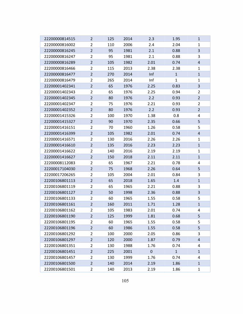
105

22200000814515  2  125  2014  2.3  1.95  1 

22200000816002  2  110  2006  2.4  2.04  1 

22200000816245  2  95  1981  2.1  0.88  3 

22200000816247  2  95  1981  2.1  0.88  3 

22200000816289  2  105  1982  2.01  0.74  4 

22200000816466  2  115  2013  2.38  2.38  1 

22200000816477  2  270  2014  Inf  1  1 

22200000816479  2  265  2014  Inf  1  1 

22200001402341  2  65  1976  2.25  0.83  3 

22200001402343  2  65  1976  2.25  0.94  2 

22200001402345  2  80  1976  2.2  0.93  2 

22200001402347  2  75  1976  2.21  0.93  2 

22200001402352  2  80  1976  2.2  0.93  2 

22200001415326  2  100  1970  1.38  0.8  4 

22200001415327  2  90  1970  2.35  0.66  5 

22200001416151  2  70  1960  1.26  0.58  5 

22200001416399  2  105  1982  2.01  0.74  4 

22200001416571  2  130  2016  2.26  2.26  1 

22200001416610  2  135  2016  2.23  2.23  1 

22200001416622  2  140  2016  2.19  2.19  1 

22200001416627  2  150  2018  2.11  2.11  1 

22200008112083  2  65  1967  2.21  0.78  4 

22200017104030  2  75  1968  2.26  0.64  5 

22200017206265  2  105  2004  2.01  0.84  3 

22200106801113  2  65  2018  1.65  1.4  1 

22200106801119  2  65  1965  2.21  0.88  3 

22200106801127  2  50  1998  2.36  0.88  3 

22200106801133  2  60  1965  1.55  0.58  5 

22200106801161  2  160  2011  1.71  1.28  1 

22200106801162  2  105  1983  2.01  0.74  4 

22200106801190  2  125  1999  1.81  0.68  5 

22200106801195  2  60  1965  1.55  0.58  5 

22200106801196  2  60  1986  1.55  0.58  5 

22200106801292  2  100  2000  2.05  0.86  3 

22200106801297  2  120  2000  1.87  0.79  4 

22200106801351  2  130  1988  1.76  0.74  4 

22200106801451  2  225  2001  0  1  1 

22200106801457  2  130  1999  1.76  0.74  4 

22200106801500  2  140  2014  2.19  1.86  1 

22200106801501  2  140  2013  2.19  1.86  1 

106

22200106801508  2  140  2014  2.19  1.86  1 

22200106802057  2  80  1976  1.33  0.77  4 

22200106802330  2  125  1983  1.81  0.68  5 

22200106802379  2  145  1991  1.56  0.9  3 

22200106802492  2  160  2010  2.02  1.72  1 

22200106802558  2  90  2017  2.49  2.49  1 

22200226602061  2  100  1991  2.05  0.76  4 

22200226602072  2  75  1994  2.21  0.93  2 

22200237405292  2  185  1975  0  1  1 

22200237405446  2  140  1996  1.66  0.7  5 

022200ZW3190001  2  80  1980  2.2  0.93  2 

22490001306327  2  70  2010  2.42  2.06  1 

22490001308093  2  95  1996  2.1  0.88  3