A Game-Theoretic Framework for Studying Truck Platooning Incentives

Farhad Farokhi and Karl H. Johansson

Abstract— An atomic congestion game with two types ofagents, cars and trucks, is used to model the traffic flow ona road over certain time intervals. In this game, the driversmake a trade-off between the time they choose to use theroad, the average velocity of the flow at that time, and thedynamic congestion tax that they are paying to use the road.The trucks have platooning capabilities and therefore, have anincentive for using the road at the same time as their peers. Thedynamics and equilibria of this game-theoretic model for theinteraction between car traffic and truck platooning incentivesare investigated. We use traffic data from Stockholm to validatethe modeling assumptions and extract reasonable parametersfor the simulations. We perform a comprehensive simulationstudy to understand the influence of various factors, such asthe percentage of the trucks that are equipped with platooningdevices on the properties of the pure strategy Nash equilibriumthat is learned using a joint strategy fictitious play.

I. INTRODUCTION

Urban traffic congestion creates many problems, such as,

increased transportation delays and fuel consumption, air

pollution, and dampened economic growth in heavily con-

gested areas [1]–[3]. To circumvent part of these issues, the

local governments in some urban areas introduced congestion

taxes to manage the traffic congestion over existing infras-

tructures. For instance, Stockholm implemented a congestion

taxing system in August, 2007 after a seven-month trial

period between January–July, 2006. A survey of the influence

of the congestion taxes over the trial period can be found

in [4], which technically shows significant improvements in

travel times as well as favorable economic and environmen-

tal effects. Behavioral aspects and other influences of the

Stockholm congestion taxing system is discussed in [5]–[8].

In parallel to reducing the congestion, we can employ

other means to improve the fuel efficiency and decrease

the carbon emission [1]. Trucks or heavy-duty vehicles

can improve their fuel efficiency by platooning with their

peers. In [9], the authors report 4.7%-7.7% reduction in

the fuel consumption (depending on the distance between

the vehicles among other factors) when two identical trucks

move close to each other at 70 km/h. The fuel saving is

mainly due to the reduced air drag force on the vehicles when

they form platoons. In a futuristic scenario where several

trucks are equipped with platooning devices, they are able

to save fuel by cooperating with each other. Implementing

truck platooning in a large-scale setup is not easy since

a global decision-maker might become complex and the

vehicles can belong to competing entities. It is interesting to

The authors are with ACCESS Linnaeus Center, School of ElectricalEngineering, KTH Royal Institute of Technology, SE-100 44 Stockholm,Sweden. E-mails: {farakhi,kallej}@kth.se

The work was supported by the Swedish Research Council, the Knut andAlice Wallenberg Foundation, and the iQFleet project.

instead study if a desirable behavior can emerge from simple

local strategies. In this paper, we consider such a case where

the traffic flow can be modeled as a congestion game and

the desired behavior corresponds to an equilibrium of this

game.

In this paper, we model the traffic flow at non-overlapping

intervals of the day using an atomic1 congestion game with

two types of agents. The first type of agents are cars or trucks

that do not have platooning equipments. They optimize

their utility, which is a sum of the penalty for deviating

from their preferred time interval for using the road, the

average velocity of the traffic flow along the road, and the

congestion tax that they pay for using the road at that time

interval. The second type of agents are trucks equipped with

platooning devices. In addition to the above mentioned term,

they have an incentive for using the road with other second-

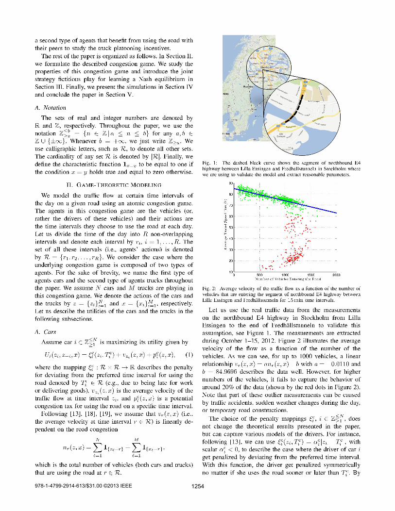
type agents. We model the average velocity of the flow at

each time interval as a linear function of the number of the

vehicles that are using the road at that time interval. We

use real traffic data from the northbound E4 highway from

Lilla Essingen to the end of Fredhallstunneln in Stockholm,

Sweden (see Figure 1) to validate this modeling assumption.

We show that the atomic congestion game admits at least

one pure strategy Nash equilibrium under an appropriate

congestion tax policy for the first type of agents. Then, we

use joint strategy fictitious play to learn a Nash equilibrium.

Intuitively, we interpret the learning algorithm as the way

drivers decide on a daily basis to choose the time interval

on which they are using the road by optimizing their utility

given the history of their actions. Iterating over days, the

drivers’ decisions (i.e., the profile of the learning algorithm)

converges almost surely to a pure strategy Nash equilibrium.

Using the parameters extracted from the real congestion data,

we construct a simulation setup to study the performance of

the joint strategy fictitious play as well as the properties of

the captured Nash equilibrium. For instance, we study the

robustness to perturbations of the learning algorithm, e.g.,

accidents along the road, sudden weather changes in a day,

or temporary road constructions.

Modeling the traffic flow using congestion games and

studying their efficiency are well-known problems (see [11]–

[17] among many other studies). However, contrary to all

these studies, we employ an atomic congestion game with

two types of agents to study the possibility of platooning

and its incentives when dealing with strategic drivers. A

model that inspired our traffic flow modeling was introduced

in [13]. In the current paper, we expand this model by adding

1We use the term atomic to emphasize the fact that we are not dealingwith a continuum of players or fractional flows when modeling the trafficflow as a congestion game [10], [11].

Proceedings of the 16th International IEEE Annual Conference onIntelligent Transportation Systems (ITSC 2013), The Hague, TheNetherlands, October 6-9, 2013

TuB7.1

978-1-4799-2914-613/$31.00 ©2013 IEEE 1253

978-1-4799-2914-613/$31.00 ©2013 IEEE 1254

increasing |αci |, she becomes less flexible. Another penalty

function is ξci (zi, Tci ) = αc

i max(zi−T ci , 0), which penalizes

the driver of car i only for being late. For the simulations in

the paper, we assume that all vehicles use the first penalty

mapping.

B. Trucks

We assume truck j ∈ Z≤M≥1 is maximizing the utility

Vj(xj , x−j , z) = ξtj(xj , Ttj ) + vxj

(z, x)

+ βvxj(z, x)g(mxj

(x)) + pti(z, x),(2)

where, similar to the utilities of the cars, ξtj(xj , Ttj ) is the

penalty for deviating from the preferred time T tj for using

the road, vxj(z, x) is the average velocity of the traffic

flow, and pti(z, x) is a potential congestion tax for using

the road at time interval xj . Trucks have an extra term

βvxj(z, x)g(mxj

(x)) in their utility because of their benefit

in using the road at the same time as the other trucks. Here,

g : Z≤M≥1 → R is a nondecreasing function and mr(x) =

∑M

ℓ=1 1{xℓ=r} is the number of trucks that are using the

road at time interval r ∈ R. The increased utility can be

justified by the fact that whenever there are many trucks

on the road at the same time interval, they can potentially

form platoons to increase the fuel efficiency. It should be

noted that this extra utility is a function of the average

velocity of the flow since the trucks cannot save a significant

amount of fuel through platooning whenever traveling at

low velocities (see [9], [20] and the references therein for

a discussion on this matter). The function g : Z≤M≥1 → R

describes the dependency of the platooning incentive on the

number of trucks that are using the road at that time interval.

Again, the choice of this function would not change the

mathematical results presented in this paper, but it can help

us to capture the relationship between the fuel saving and

the number of the trucks on the road in a more realistic

fashion. For instance, g(mxj(x)) = mxj

(x) shows that the

vehicles can even benefit from a low number of trucks but

g(mxj(x)) = mxj

(x)1mxj(x)≥τ describe the case where

the trucks do not benefit until they reach a critical number

τ ∈ Z≥1. For the simulations in this paper, we assume that

all trucks use the first mapping.

Notice that in the utilities (1) and (2), we introduced

potential congestion taxes for the cars and the trucks. They

are used to ensure that the described game is a potential

game. Such a game admits at least one pure strategy Nash

equilibrium and we can use joint strategy fictitious play to

learn an equilibrium.

III. LEARNING A PURE STRATEGY NASH EQUILIBRIUM

In this section, we introduce the joint strategy fictitious

play [21] to learn a pure strategy Nash equilibrium of the

congestion game introduced in Section II. In the reminder

of this paper, we assume that the trucks do not pay any

congestion tax; i.e., ptj(z, x) = 0 for all j ∈ Z≤M≥1 . Let us

start by proving that the congestion game is a potential game

under an appropriate congestion tax policy for cars.

LEMMA 1: Let each car i ∈ Z≤N≥1 pay the congestion tax

pci (z, x) = aβ

mzi(x)

∑

ℓ=1

g(ℓ), (3)

for using the road at time interval zi ∈ R. Then, the atomic

congestion game with the utilities introduced in (1) and (2)

is a potential game2 with the potential function Φ(x, z) =∑4

k=1 Φk(x, z) where

Φ1(x, z) =

N∑

i=1

ξci (zi, Tci ) +

M∑

j=1

ξtj(xj , Ttj ),

Φ2(x, z) =

R∑

r=1

nr(x,z)∑

k=1

(ak + b),

Φ3(x, z) =R∑

r=1

β(anr(x, z) + b)

mr(x)∑

ℓ=1

g(ℓ),

Φ4(x, z) = −aβ

R∑

r=1

mr(x)∑

ℓ=1

ℓ−1∑

k=1

g(k).

Furthermore, this game admits at least one pure strategy

Nash equilibrium3.

Proof: The proof of this lemma follows the same line

of reasoning as in the proof of Proposition 4.1 in [13]. Let us

start by analyzing the trucks. If xj = x′j , the result trivially

holds. Consequently, we consider the case where xj 6= x′j ,

which results in

Φ(xj ,x−j ,z)−Φ(x′j ,x−j ,z)=

4∑

k=1

Φk(xj ,x−j ,z)−Φk(x′j ,x−j ,z).

We continue the proof by considering each term of this

summation separately. For the first term, clearly, we have

Φ1(xj , x−j , z)− Φ1(x′j , x−j , z) = ξtj(xj , T

tj )− ξtj(x

′j , T

tj ).

Let us define x′ = (x′j , x−j). For the second term, we have

Φ2(xj , x−j , z)− Φ2(x′j , x−j , z)

=

R∑

r=1

nr(x,z)∑

k=1

(ak + b)−

R∑

r=1

nr(x′,z)

∑

k=1

(ak + b)

=

nxj(x,z)

∑

k=1

(ak + b) +

nx′

j(x,z)

∑

k=1

(ak + b)

−

nxj(x′,z)∑

k=1

(ak + b)−

nx′

j(x′,z)∑

k=1

(ak + b),

2The introduced congestion game is a potential game with potentialfunction Φ : RN × RM → R if Φ(x, zi, z−i) − Φ(x, z′i, z−i) =Ui(zi, z−i, x) − Ui(z

′i, z−i, x) and Φ(xj , x−j , z) − Φ(x′

j , x−j , z) =

Vj(xj , x−j , z) − Vj(x′j , x−j , z) for all i ∈ Z

≤N

≥1and j ∈ Z

≤M

≥1. We

would like to refer the interested readers to [22] to study potential games.3For the introduced congestion game, a pure strategy Nash equilibrium

is a pair (z, x) ∈ RN × RM such that Ui(zi, z−i, x) ≥ Ui(z′i, z−i, x)

for all z′i ∈ R and i ∈ Z≤N

≥1and Vj(xj , x−j , z) ≥ Vj(x

′j , x−j , z) for

all x′j ∈ R and j ∈ Z

≤M

≥1. We would like to refer the interested readers

to [23] for a comprehensive review of the game theoretic concepts.

978-1-4799-2914-613/$31.00 ©2013 IEEE 1255

where the second equality holds because of the fact that

nr(x, z) = nr(x′, z) for all r 6= xj , x

′j . Note that

nxj(x′, z) = nxj

(x, z)−1, nx′

j(x, z) = nx′

j(x′, z)−1, (4)

and as a result,

Φ2(xj , x−j , z)− Φ2(x′j , x−j , z)

= (anxj(z, x) + b)− (anx′

j(z, x′) + b).

For the third term, we get the identity in (5), on top of the

next page, where the last equality follows from using (4)

and the fact that mxj(x′) = mxj

(x) − 1 and mx′

j(x) =

mx′

j(x′)−1. Finally, using the same argument as in the case

of the second term and the third term, we get

Φ4(xj , x−j , z)− Φ4(x′j , x−j , z)

= −aβ

mxj(x)−1∑

ℓ=1

g(ℓ) + aβ

mx′

j(x′)−1∑

ℓ=1

g(ℓ).

Combining all these differences, we get

Φ(xj , x−j , z)− Φ(x′j , x−j , z)

=β(anxj(x, z) + b)g(mxj

(x))

− β(anx′

j(x′, z) + b)g(mx′

j(x′))

+ ξtj(xj , Ttj )− ξtj(x

′j , T

tj )

+ (anxj(z, x) + b)− (anx′

j(z, x′) + b)

=Vj(xj , x−j , z)− Vj(x′j , x−j , z).

Now, let us prove this fact for the cars as well. If zi = z′i,the result trivially holds. Thus, we investigate the case where

zi 6= z′i. Similarly, we consider each term of the summation

separately. For the first term, we have

Φ1(x, zi, z−i)− Φ1(x, z′i, z−i) = ξci (zi, T

ci )− ξci (z

′i, T

ci ).

We define the notation z′ = (z′i, z−i). Following a similar

reasoning as in the case of the trucks, for the second and the

third terms, we get

Φ2(x, zi, z−i)− Φ2(x, z′i, z−i)

= (anzi(z, x) + b)− (anz′

i(z′, x) + b),

and

Φ3(x, zi, z−i)− Φ3(x, z′i, z−i)

= aβ

mzi(x)

∑

ℓ=1

g(ℓ)− aβ

mz′i(x)

∑

ℓ=1

g(ℓ).

For the forth term, we get Φ4(x, zi, z−i)−Φ4(x, z′i, z−i) = 0

since this term is only a function of x which is not changed.

Again, combining all these differences, we get

Φ(x, zi, z−i)− Φ(x, z′i, z−i)

= (anzi(z, x) + b)− (anz′

i(z′, x) + b)

+ ξci (zi, Tci )− ξci (z

′i, T

ci )

+ aβ

mzi(x)

∑

ℓ=1

g(ℓ)− aβ

mz′i(x)

∑

ℓ=1

g(ℓ)

=Ui(zi, z−i, x)− Ui(z′i, z−i, x).

Procedure 1 The joint strategy fictitious play for learning a Nashequilibrium of the introduced congestion game.

Input: p ∈ (0, 1)Output: (x∗, z∗)

1: for t = 0, 1, . . . do2: for i = 1, . . . , N do

3: Calculate z′i ∈ argmaxr∈R Ui(r; t− 1)4: if Ui(z

′i, z−i(t − 1), x(t − 1)) ≤ Ui(zi(t − 1), z−i(t −

1), x(t− 1)) then5: zi(t)← zi(t− 1)6: else7: With probability 1 − p, zi(t) ← zi(t − 1), otherwise

zi(t)← z′i8: end if9: for j = 1, . . . ,M do

10: Calculate x′j ∈ argmaxr∈R Vj(r; t− 1)

11: if Vj(z(t− 1), x′j , x−j(t− 1)) ≤ Vj(z(t− 1), xj(t−

1), x−j(t− 1)) then12: xj(t)← xj(t− 1)13: else14: With probability 1−p, xj(t)← xj(t−1), otherwise

xj(t)← x′j

15: end if16: end for17: end for

18: end for

Finally, note that every potential game admits at least one

pure strategy Nash equilibrium [22].

Recall that a game that is a potential game admits at least a

pure strategy Nash equilibrium and we can use joint strategy

fictitious play to learn a Nash equilibrium [21], [22].

Note that when g : Z≤M≥1 → R is linear, then pci (z, x) at

each time interval grows quadratically with the number of

the trucks that are using the road at that interval. Therefore,

the cars avoid the time intervals that the trucks use to travel.

Now, we briefly introduce the joint strategy fictitious play

and analyze its convergence for the introduced congestion

game. The agents calculate an average utility given the

history of the actions. At time step t ∈ Z≥0, car i ∈ Z≤N≥1

computes Ui(r; t) using the recursive equation

Ui(r; t) = (1− λt)Ui(r; t− 1) + λtUi(r, z−i(t), x(t)), (6)

with the initial condition Ui(r;−1) = ξci (r, Tci ) for all r ∈

R. In (6), λt ∈ (0, 1] is a forgetting factor which captures

the extent that the agents forget the actions from the past.

If λt = 1, the agents are myopic (i.e., only consider the

actions from the previous time step) while if λt = 1/t, the

agents value the whole history at the same level. Following

the same approach, truck j ∈ Z≤M≥1 calculates Vj(r; t) using

the recursive equation

Vj(r; t) = (1− λt)Vj(r; t− 1) + λtVj(r, x−j(t), z(t)),

with Vj(r;−1) = ξtj(r, Ttj ) for all r ∈ R. Procedure 1 shows

the joint strategy fictitious play for the introduced conges-

tion game. This numerical procedure converges to a Nash

equilibrium of the congestion game under the congestion tax

policy (3).

THEOREM 2: Let the actions of the agents be generated

by the joint strategy fictitious play in Procedure 1. Then,

978-1-4799-2914-613/$31.00 ©2013 IEEE 1256

Φ3(xj , x−j , z)− Φ3(x′j , x−j , z) =

R∑

r=1

β(anr(x, z) + b)

mr(x)∑

ℓ=1

g(ℓ)−R∑

r=1

β(anr(x′, z) + b)

mr(x′)

∑

ℓ=1

g(ℓ)

= β(anxj(x, z) + b)

mxj(x)

∑

ℓ=1

g(ℓ) + β(anx′

j(x, z) + b)

mx′

j(x)

∑

ℓ=1

g(ℓ)

− β(anxj(x′, z) + b)

mxj(x′)

∑

ℓ=1

g(ℓ)− β(anx′

j(x′, z) + b)

mx′

j(x′)

∑

ℓ=1

g(ℓ)

= β(anxj(x, z) + b)g(mxj

(x))− β(anx′

j(x′, z) + b)g(mx′

j(x′))

+ aβ

mxj(x)−1∑

ℓ=1

g(ℓ)− aβ

mx′

j(x′)−1∑

ℓ=1

g(ℓ),

(5)

these actions converge almost surely to a pure strategy Nash

equilibrium of the atomic congestion game if the cars pay

the congestion tax (3).

Proof: The proof is a consequence of combining The-

orem 3.1 in [21] with Lemma 1.

IV. NUMERICAL EXAMPLE

Let us assume that N = 10000 cars and M = 100trucks are using the segment of the highway illustrated in

Figure 1 from 7:00am to 9:00am on a daily basis. We

divide the time horizon into eight equal non-overlapping

intervals. Hence, we fix the action set as R = {1, . . . , 8},

where each number represents an interval of 15min. Let T ci ,

i ∈ Z≤N≥1 , be randomly chosen from the set R using the

discrete distribution

P{T ci = n} =

1/6, n = 2, 4,1/4, n = 3,1/12, otherwise.

Let us also use a similar probability distribution to extract

T tj , j ∈ Z

≤M≥1 . Hence, we consider the case where the drivers

statistically prefer to use the road at r = 3 which corresponds

to 7:30am to 7:45am. Let αci , i ∈ Z

≤N≥1 , and αt

j , j ∈ Z≤M≥1 , be

randomly generated following a uniform distribution within

the interval [−7.5,−2.5]. Finally, let a = −0.0110 and b =84.9696 as discussed in Section II.

A. Learning Algorithm Performance

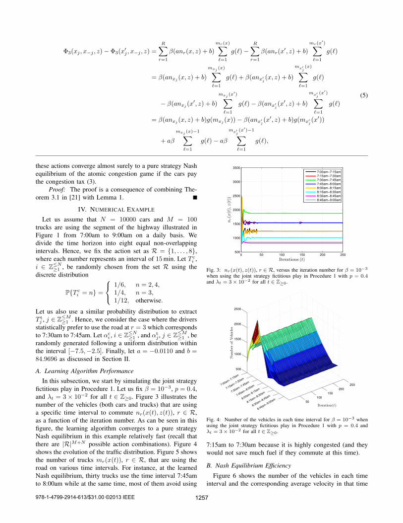
In this subsection, we start by simulating the joint strategy

fictitious play in Procedure 1. Let us fix β = 10−3, p = 0.4,

and λt = 3 × 10−2 for all t ∈ Z≥0. Figure 3 illustrates the

number of the vehicles (both cars and trucks) that are using

a specific time interval to commute nr(x(t), z(t)), r ∈ R,

as a function of the iteration number. As can be seen in this

figure, the learning algorithm converges to a pure strategy

Nash equilibrium in this example relatively fast (recall that

there are |R|M+N possible action combinations). Figure 4

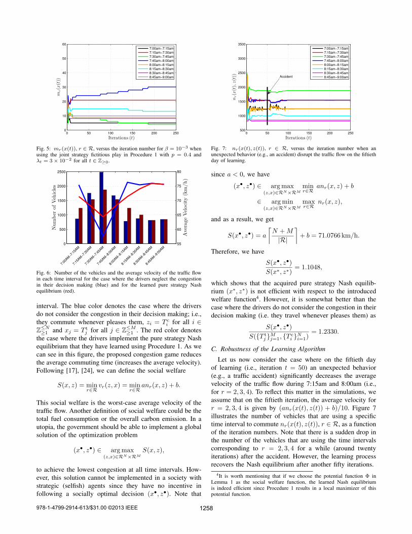
shows the evolution of the traffic distribution. Figure 5 shows

the number of trucks mr(x(t)), r ∈ R, that are using the

road on various time intervals. For instance, at the learned

Nash equilibrium, thirty trucks use the time interval 7:45am

to 8:00am while at the same time, most of them avoid using

0 50 100 150 200 250500

1000

1500

2000

2500

3000

3500

nr(x(t),z(t))

Iterations (t)

7:00am−7:15am

7:15am−7:30am

7:30am−7:45am

7:45am−8:00am

8:00am−8:15am

8:15am−8:30am

8:30am−8:45am

8:45am−9:00am

Fig. 3: nr(x(t), z(t)), r ∈ R, versus the iteration number for β = 10−3

when using the joint strategy fictitious play in Procedure 1 with p = 0.4and λt = 3× 10−2 for all t ∈ Z≥0.

50

100

150

200

250

500

1000

1500

2000

2500

Iteration(t)8:4

5am−9:0

0am

8:30am

−8:45am

8:15am

−8:30am

8:00am

−8:15am

7:45am

−8:00am

7:30am

−7:45am

7:15am

−7:30am

7:00am

−7:15am

Number

ofVehicles

Fig. 4: Number of the vehicles in each time interval for β = 10−3 whenusing the joint strategy fictitious play in Procedure 1 with p = 0.4 andλt = 3× 10−2 for all t ∈ Z≥0.

7:15am to 7:30am because it is highly congested (and they

would not save much fuel if they commute at this time).

B. Nash Equilibrium Efficiency

Figure 6 shows the number of the vehicles in each time

interval and the corresponding average velocity in that time

978-1-4799-2914-613/$31.00 ©2013 IEEE 1257

0 50 100 150 200 2500

10

20

30

40

50

60

mr(x(t))

Iterations (t)

7:00am−7:15am

7:15am−7:30am

7:30am−7:45am

7:45am−8:00am

8:00am−8:15am

8:15am−8:30am

8:30am−8:45am

8:45am−9:00am

Fig. 5: mr(x(t)), r ∈ R, versus the iteration number for β = 10−3 whenusing the joint strategy fictitious play in Procedure 1 with p = 0.4 andλt = 3× 10−2 for all t ∈ Z≥0.

7:0

0AM

−7:1

5AM

7:1

5AM

−7:3

0AM

7:3

0AM

−7:4

5AM

7:4

5AM

−8:0

0AM

8:0

0AM

−8:1

5AM

8:1

5AM

−8:3

0AM

8:3

0AM

−8:4

5AM

8:4

5AM

−9:0

0AM

Number

ofVeh

icles

0

500

1000

1500

2000

2500

AverageVelocity

(km/h)

55

60

65

70

75

80

Fig. 6: Number of the vehicles and the average velocity of the traffic flowin each time interval for the case where the drivers neglect the congestionin their decision making (blue) and for the learned pure strategy Nashequilibrium (red).

interval. The blue color denotes the case where the drivers

do not consider the congestion in their decision making; i.e.,

they commute whenever pleases them, zi = T ci for all i ∈

Z≤N≥1 and xj = T t

j for all j ∈ Z≤M≥1 . The red color denotes

the case where the drivers implement the pure strategy Nash

equilibrium that they have learned using Procedure 1. As we

can see in this figure, the proposed congestion game reduces

the average commuting time (increases the average velocity).

Following [17], [24], we can define the social welfare

S(x, z) = minr∈R

vr(z, x) = minr∈R

anr(x, z) + b.

This social welfare is the worst-case average velocity of the

traffic flow. Another definition of social welfare could be the

total fuel consumption or the overall carbon emission. In a

utopia, the government should be able to implement a global

solution of the optimization problem

(x•, z•) ∈ argmax(z,x)∈RN×RM

S(x, z),

to achieve the lowest congestion at all time intervals. How-

ever, this solution cannot be implemented in a society with

strategic (selfish) agents since they have no incentive in

following a socially optimal decision (x•, z•). Note that

0 50 100 150 200 250500

1000

1500

2000

2500

3000

3500

nr(x(t),z(t))

Iterations (t)

7:00am−7:15am

7:15am−7:30am

7:30am−7:45am

7:45am−8:00am

8:00am−8:15am

8:15am−8:30am

8:30am−8:45am

8:45am−9:00amAccident

Fig. 7: nr(x(t), z(t)), r ∈ R, versus the iteration number when anunexpected behavior (e.g., an accident) disrupt the traffic flow on the fiftiethday of learning.

since a < 0, we have

(x•, z•) ∈ argmax(z,x)∈RN×RM

minr∈R

anr(x, z) + b

∈ argmin(z,x)∈RN×RM

maxr∈R

nr(x, z),

and as a result, we get

S(x•, z•) = a

⌈

N +M

|R|

⌉

+ b = 71.0766 km/h.

Therefore, we have

S(x•, z•)

S(x∗, z∗)= 1.1048,

which shows that the acquired pure strategy Nash equilib-

rium (x∗, z∗) is not efficient with respect to the introduced

welfare function4. However, it is somewhat better than the

case where the drivers do not consider the congestion in their

decision making (i.e. they travel whenever pleases them) as

S(x•, z•)

S({T tj }

Mj=1, {T

ci }

Ni=1)

= 1.2330.

C. Robustness of the Learning Algorithm

Let us now consider the case where on the fiftieth day

of learning (i.e., iteration t = 50) an unexpected behavior

(e.g., a traffic accident) significantly decreases the average

velocity of the traffic flow during 7:15am and 8:00am (i.e.,

for r = 2, 3, 4). To reflect this matter in the simulations, we

assume that on the fiftieth iteration, the average velocity for

r = 2, 3, 4 is given by (anr(x(t), z(t)) + b)/10. Figure 7

illustrates the number of vehicles that are using a specific

time interval to commute nr(x(t), z(t)), r ∈ R, as a function

of the iteration numbers. Note that there is a sudden drop in

the number of the vehicles that are using the time intervals

corresponding to r = 2, 3, 4 for a while (around twenty

iterations) after the accident. However, the learning process

recovers the Nash equilibrium after another fifty iterations.

4It is worth mentioning that if we choose the potential function Φ inLemma 1 as the social welfare function, the learned Nash equilibriumis indeed efficient since Procedure 1 results in a local maximizer of thispotential function.

978-1-4799-2914-613/$31.00 ©2013 IEEE 1258

Number

ofTrucks

7:0

0am

−7:1

5am

7:1

5am

−7:3

0am

7:3

0am

−7:4

5am

7:4

5am

−8:0

0am

8:0

0am

−8:1

5am

8:1

5am

−8:3

0am

8:3

0am

−8:4

5am

8:4

5am

−9:0

0am

0

20

40

60

80

100

120

β = 0.0e+ 00β = 1.0e− 03β = 2.0e− 03β = 3.0e− 03β = 4.0e− 03

Fig. 8: Number of the trucks in each time interval for various choices ofthe coefficient β.

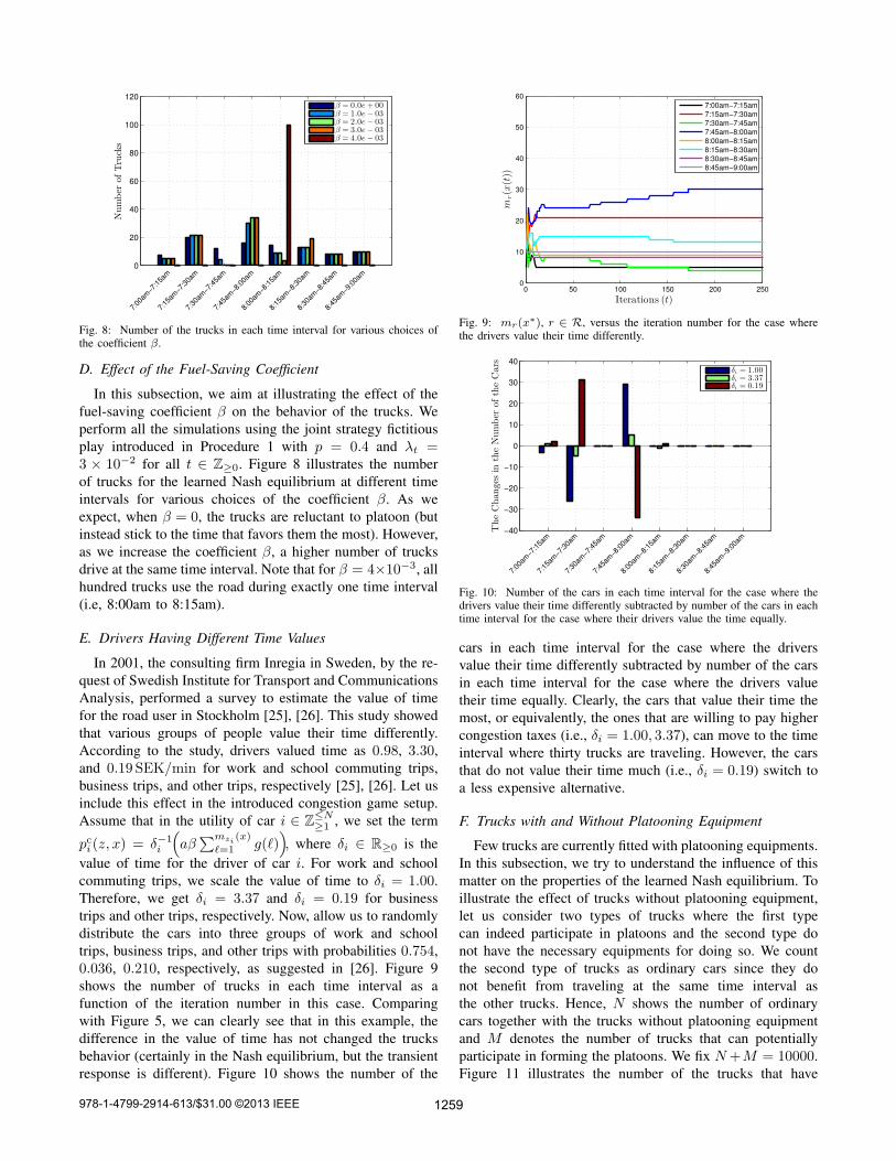
D. Effect of the Fuel-Saving Coefficient

In this subsection, we aim at illustrating the effect of the

fuel-saving coefficient β on the behavior of the trucks. We

perform all the simulations using the joint strategy fictitious

play introduced in Procedure 1 with p = 0.4 and λt =3 × 10−2 for all t ∈ Z≥0. Figure 8 illustrates the number

of trucks for the learned Nash equilibrium at different time

intervals for various choices of the coefficient β. As we

expect, when β = 0, the trucks are reluctant to platoon (but

instead stick to the time that favors them the most). However,

as we increase the coefficient β, a higher number of trucks

drive at the same time interval. Note that for β = 4×10−3, all

hundred trucks use the road during exactly one time interval

(i.e, 8:00am to 8:15am).

E. Drivers Having Different Time Values

In 2001, the consulting firm Inregia in Sweden, by the re-

quest of Swedish Institute for Transport and Communications

Analysis, performed a survey to estimate the value of time

for the road user in Stockholm [25], [26]. This study showed

that various groups of people value their time differently.

According to the study, drivers valued time as 0.98, 3.30,

and 0.19 SEK/min for work and school commuting trips,

business trips, and other trips, respectively [25], [26]. Let us

include this effect in the introduced congestion game setup.

Assume that in the utility of car i ∈ Z≤N≥1 , we set the term

pci (z, x) = δ−1i

(

aβ∑mzi

(x)

ℓ=1 g(ℓ))

, where δi ∈ R≥0 is the

value of time for the driver of car i. For work and school

commuting trips, we scale the value of time to δi = 1.00.

Therefore, we get δi = 3.37 and δi = 0.19 for business

trips and other trips, respectively. Now, allow us to randomly

distribute the cars into three groups of work and school

trips, business trips, and other trips with probabilities 0.754,

0.036, 0.210, respectively, as suggested in [26]. Figure 9

shows the number of trucks in each time interval as a

function of the iteration number in this case. Comparing

with Figure 5, we can clearly see that in this example, the

difference in the value of time has not changed the trucks

behavior (certainly in the Nash equilibrium, but the transient

response is different). Figure 10 shows the number of the

0 50 100 150 200 2500

10

20

30

40

50

60

mr(x(t))

Iterations (t)

7:00am−7:15am

7:15am−7:30am

7:30am−7:45am

7:45am−8:00am

8:00am−8:15am

8:15am−8:30am

8:30am−8:45am

8:45am−9:00am

Fig. 9: mr(x∗), r ∈ R, versus the iteration number for the case wherethe drivers value their time differently.

TheChanges

intheNumber

oftheCars

7:0

0am

−7:1

5am

7:1

5am

−7:3

0am

7:3

0am

−7:4

5am

7:4

5am

−8:0

0am

8:0

0am

−8:1

5am

8:1

5am

−8:3

0am

8:3

0am

−8:4

5am

8:4

5am

−9:0

0am

−40

−30

−20

−10

0

10

20

30

40

δi = 1.00δi = 3.37δi = 0.19

Fig. 10: Number of the cars in each time interval for the case where thedrivers value their time differently subtracted by number of the cars in eachtime interval for the case where their drivers value the time equally.

cars in each time interval for the case where the drivers

value their time differently subtracted by number of the cars

in each time interval for the case where the drivers value

their time equally. Clearly, the cars that value their time the

most, or equivalently, the ones that are willing to pay higher

congestion taxes (i.e., δi = 1.00, 3.37), can move to the time

interval where thirty trucks are traveling. However, the cars

that do not value their time much (i.e., δi = 0.19) switch to

a less expensive alternative.

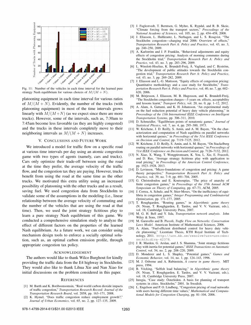
F. Trucks with and Without Platooning Equipment

Few trucks are currently fitted with platooning equipments.

In this subsection, we try to understand the influence of this

matter on the properties of the learned Nash equilibrium. To

illustrate the effect of trucks without platooning equipment,

let us consider two types of trucks where the first type

can indeed participate in platoons and the second type do

not have the necessary equipments for doing so. We count

the second type of trucks as ordinary cars since they do

not benefit from traveling at the same time interval as

the other trucks. Hence, N shows the number of ordinary

cars together with the trucks without platooning equipment

and M denotes the number of trucks that can potentially

participate in forming the platoons. We fix N+M = 10000.

Figure 11 illustrates the number of the trucks that have

978-1-4799-2914-613/$31.00 ©2013 IEEE 1259

Number

ofTruckswithPlatoon

ingEquipment

7:0

0am

−7:1

5am

7:1

5am

−7:3

0am

7:3

0am

−7:4

5am

7:4

5am

−8:0

0am

8:0

0am

−8:1

5am

8:1

5am

−8:3

0am

8:3

0am

−8:4

5am

8:4

5am

−9:0

0am

0

20

40

60

80

100

120

140

M/(N +M) = 0.5%M/(N +M) = 1%M/(N +M) = 1.5%M/(N +M) = 2%M/(N +M) = 2.5%

Fig. 11: Number of the vehicles in each time interval for the learned purestrategy Nash equilibrium for various choices of M/(M +N).

platooning equipment in each time interval for various ratios

of M/(M +N). Evidently, the number of the trucks (with

platooning equipment) in most of the time intervals grows

linearly with M/(M+N) (as we expect since there are more

trucks). However, some of the intervals, such as, 7:30am to

7:45am become less favorable (as they are highly congested)

and the trucks in these intervals completely move to their

neighboring intervals as M/(M +N) increases.

V. CONCLUSIONS AND FUTURE WORK

We introduced a model for traffic flow on a specific road

at various time intervals per day using an atomic congestion

game with two types of agents (namely, cars and trucks).

Cars only optimize their trade-off between using the road

at the time they prefer, the average velocity of the traffic

flow, and the congestion tax they are paying. However, trucks

benefit from using the road at the same time as the other

trucks. We motivated this extra utility using an increased

possibility of platooning with the other trucks and as a result,

saving fuel. We used congestion data from Stockholm to

validate some of the assumptions in the modeling (i.e., linear

relationship between the average velocity of commuting and

the number of the vehicles that are using the road at that

time). Then, we used the joint strategy fictitious play to

learn a pure strategy Nash equilibrium of this game. We

conducted a comprehensive simulation study to analyze the

effect of different factors on the properties of the learned

Nash equilibrium. As a future work, we can consider using

mechanism design tools to enforce a socially optimal solu-

tion, such as, an optimal carbon emission profile, through

appropriate congestion tax policy.

ACKNOWLEDGEMENT

The authors would like to thank Wilco Burghout for kindly

providing the traffic data from the E4 highway in Stockholm.

They would also like to thank Lihua Xie and Nan Xiao for

initial discussions on the problem considered in this paper.

REFERENCES

[1] M. Barth and K. Boriboonsomsin, “Real-world carbon dioxide impactsof traffic congestion,” Transportation Research Record: Journal of the

Transportation Research Board, vol. 2058, pp. 163–171, 2008.[2] K. Hymel, “Does traffic congestion reduce employment growth?,”

Journal of Urban Economics, vol. 65, no. 2, pp. 127–135, 2009.

[3] J. Fuglestvedt, T. Berntsen, G. Myhre, K. Rypdal, and R. B. Skeie,“Climate forcing from the transport sectors,” Proceedings of the

National Academy of Sciences, vol. 105, no. 2, pp. 454–458, 2008.[4] J. Eliasson, L. Hultkrantz, L. Nerhagen, and L. S. Rosqvist, “The

Stockholm congestion—charging trial 2006: Overview of effects,”Transportation Research Part A: Policy and Practice, vol. 43, no. 3,pp. 240–250, 2009.

[5] A. Karlstrom and J. P. Franklin, “Behavioral adjustments and equityeffects of congestion pricing: Analysis of morning commutes duringthe Stockholm trial,” Transportation Research Part A: Policy and

Practice, vol. 43, no. 3, pp. 283–296, 2009.[6] L. Winslott-Hiselius, K. Brundell-Freij, A. Vagland, and C. Bystrom,

“The development of public attitudes towards the Stockholm con-gestion trial,” Transportation Research Part A: Policy and Practice,vol. 43, no. 3, pp. 269–282, 2009.

[7] J. Eliasson and L.-G. Mattsson, “Equity effects of congestion pricing:Quantitative methodology and a case study for Stockholm,” Trans-

portation Research Part A: Policy and Practice, vol. 40, no. 7, pp. 602–620, 2006.

[8] M. Borjesson, J. Eliasson, M. B. Hugosson, and K. Brundell-Freij,“The Stockholm congestion charges—5 years on. effects, acceptabilityand lessons learnt,” Transport Policy, vol. 20, no. 0, pp. 1–12, 2012.

[9] A. Alam, A. Gattami, and K. H. Johansson, “An experimental studyon the fuel reduction potential of heavy duty vehicle platooning,” inProceedings of the 13th International IEEE Conference on Intelligent

Transportation Systems, pp. 306–311, 2010.[10] D. Schmeidler, “Equilibrium points of nonatomic games,” Journal of

Statistical Physics, vol. 7, no. 4, pp. 295–300, 1973.[11] W. Krichene, J. D. Reilly, S. Amin, and A. M. Bayen, “On the char-

acterization and computation of Nash equilibria on parallel networkswith horizontal queues,” in Proceedings of the 51st IEEE Conference

on Decision and Control, pp. 7119–7125, 2012.[12] W. Krichene, J. D. Reilly, S. Amin, and A. M. Bayen, “On Stackelberg

routing on parallel networks with horizontal queues,” in Proceedings of

51st IEEE Conference on Decision and Control, pp. 7126–7132, 2012.[13] N. Xiao, X. Wang, T. Wongpiromsarn, K. You, L. Xie, E. Frazzoli,

and D. Rus, “Average strategy fictitious play with application toroad pricing,” in Proceedings of the American Control Conference,pp. 1923–1928, 2013.

[14] D. Levinson, “Micro-foundations of congestion and pricing: A gametheory perspective,” Transportation Research Part A: Policy and

Practice, vol. 39, no. 7–9, pp. 691–704, 2005.[15] G. Christodoulou and E. Koutsoupias, “The price of anarchy of

finite congestion games,” in Proceedings of the 37th Annual ACM

Symposium on Theory of Computing, pp. 67–73, ACM, 2005.[16] J. Correa, A. Schulz, and N. Stier-Moses, “On the inefficiency of equi-

libria in congestion games,” Integer Programming and Combinatorial

Optimization, pp. 171–177, 2005.[17] T. Roughgarden, “Routing games,” in Algorithmic game theory

(N. Nisan, T. Roughgarden, E. Tardos, and V. V. Vazirani, eds.),vol. 18, Cambridge University Press, 2007.

[18] M. G. H. Bell and Y. Iida, Transportation network analysis. JohnWiley & Sons, 1997.

[19] M. Garavello and B. Piccoli, Traffic Flow on Networks: Conservation

Laws Model. American Institute of Mathematical Sciences, 2006.[20] A. Alam, “Fuel-efficient distributed control for heavy duty vehi-

cle platooning,” Licentiate Thesis, KTH Royal Institute of Tech-nology, 2011. http://urn.kb.se/resolve?urn=urn:nbn:

se:kth:diva-42378.[21] J. R. Marden, G. Arslan, and J. S. Shamma, “Joint strategy fictitious

play with inertia for potential games,” IEEE Transactions on Automatic

Control, vol. 54, no. 2, pp. 208–220, 2009.[22] D. Monderer and L. S. Shapley, “Potential games,” Games and

Economic Behavior, vol. 14, no. 1, pp. 124–143, 1996.[23] M. J. Osborne and A. Rubinstein, A course in game theory. MIT

press, 1994.[24] B. Vocking, “Selfish load balancing,” in Algorithmic game theory

(N. Nisan, T. Roughgarden, E. Tardos, and V. V. Vazirani, eds.),vol. 18, Cambridge University Press, 2007.

[25] Inregia, “Case study: Osterleden. A basis for planning of transportsystems in cities. Stockholm,” 2001. In Swedish.

[26] L. Engelson and P. O. Lindberg, “Congestion pricing of road networkswith users having different time values,” Mathematical and Computa-

tional Models for Congestion Charging, pp. 81–104, 2006.

978-1-4799-2914-613/$31.00 ©2013 IEEE 1260