Impact of Localized Cutbacks inAgricultural Production on

A State Economy

John B. Penson, Jr. and Murray E. Fulton

This study examines the effects that a cutback in production by Texas agriculturalproducers would have on the economic well-being of all producers and consumers in thestate's economy. To do this, a quadratic input-output model incorporating econometricestimates of final demand was developed for the Texas economy. The output of theagricultural production sectors was constrained to reflect the cutback in production. Theresults show that agricultural producers would be economically worse off than beforeonly if the producers of raw agricultural products in Texas imported their input needsfrom other geographical areas.

In 1977-78, some agricultural producerswere making strong statements about whatactions they would take if legislation were notenacted to guarantee farm prices at 100percent of parity. These actions ranged fromsending tractorcades to Washington, to cut-ting back production in an effort to dramatizethe importance of a viable agriculture to therest of the economy. Some of these actions,like the tractorcade, were carried out whileothers, such as cutting back agriculturalproduction, never materialized at the nation-al level. The regional differences noted inproducer attitudes toward cutting back pro-duction were no doubt influenced bywhether their costs of production were aboveor below the U.S. average costs of productionused in determining deficiency payments toagricultural producers.

While talk of cutbacks in production byagricultural producers has subsided since the

John B. Penson, Jr. is an Associate Professor, Depart-ment of Agricultural Economics, Texas A&M Universi-ty, College Station, Texas. Murray E. Fulton is a RhodesScholar, Oxford University, Oxford, England. The au-thors wisk to acknowledge the helpful comments pro-vided by Hovav Talpaz and Bruce Gardner. TechnicalArticle No. 15618 of the Texas Agricultural ExperimentStation.

1977-78 period, adverse developments inagriculture could renew interest in this formof action. Although it is unlikely that produc-er attitudes toward cutting back productionin periods of adverse conditions in agricul-ture would be strong at the national level,state policymakers should understand theeffects that localized cutbacks in agriculturalproduction could have on their state's grossoutput, income, indirect business taxes andemployment.

The rising cost of energy has substantiallyincreased the costs of production for thoseagricultural producers in Texas who employirrigation production practices. Approxi-mately 86 percent of all food grains and 37percent of all feed grains grown in Texas areproduced on irrigated acres. The increasingsqueeze on livestock profits - a major sourceof agricultural income in Texas - furtheradds to the economic pressures on this state'sagricultural producers. The purpose of thisstudy is to examine the short-run effects thata cutback in crop and livestock production inTexas could have on this state's generaleconomy and the economic well-being ofproducers and consumers of Texas products.This objective will be accomplished by firstdeveloping a quadratic input-output modelfor the Texas economy that accounts for the

107

Western Journal of Agricultural Economics

interdependencies between this state's ag-ricultural production sectors and other pro-duction sectors in the Texas economy. Theoutput of the agricultural production sectorsin this model will then be constrained todetermine the effects a cutback in agricultur-al production would have on agricultural andnon-agricultural producers and consumers.These effects will be illustrated by examiningthe capacity utilization rates in the non-agricultural production sectors as well as byobserving the change in producer and con-sumer surplus at the sector level. The as-sumption is initially made that processors ofraw agricultural products in Texas cannotincrease their imports of these products in aneffort to avoid the disruption to the flow ofinputs to their firms caused by the cutback inagricultural production. Finally, we shallexamine the effects on agricultural producersand others if the processors of raw agricultur-al products can increase their imports ofthese products from other geographicalareas.

Measurement of SectorInterdependencies

Interdependencies occur in an economywhen a production sector uses inputs pro-vided by other production sectors to meetthe intermediate and final demands for itsproducts. One method of accounting forthese interdependencies is to use an input-output model. First developed by Leontiefin1936, an input-output model describes asimultaneous system of linear productionfunctions for all the production sectors in themodeled economy. While the Leontief in-put-output model captures the dependencieseach production sector has upon the outputof others, it cannot be used to measure thepotential output of the economy or the effectsof a cutback in production by producers, astrike by labor or the unavailability of im-ports since it assumes perfectly elastic prod-uct and primary input supply curves.

Dorfman, Samuelson and Solow haveshown that it is possible to reformulate theLeontief input-output model as a linear pro-

108

gramming problem. Such a model can beused to estimate the potential gross output ofan economy or the effects of a cutback inproduction by producers if we constrain theoutput of each production sector by its engi-neering capacity, or the maximum outputtechnically possible in the current periodgiven its existing capital stock [Spielman andWeeks]. This is done by placing upperbounds on the production sectors equal totheir engineering capacities. The productsupply curves would be perfectly elastic onlyup to the point where the sectors reach theirengineering capacities, at which time thesecurves would become perfectly inelastic.Several problems exist, however, with usingthis model to assess the economic effects ofcutbacks in production on producers andconsumers. First, final demand is still deter-mined exogenously, suggesting consumerswould never want more than this amount nomatter what happens to product prices.Another problem is how one exogenouslydistributes total final demand among thevarious goods and services. In the real world,consumers determine how much of thesegoods and services they will want to purchasebased, in part, on their relative prices.

Harrington has shown that an input-outputmodel can be solved as a quadratic pro-gramming problem. The resulting quadraticinput-output model incorporates economet-ric estimates of linear supply functions foreach primary input and linear demand func-tions for the goods and services supplied byeach production sector. The objective of thequadratic input-output model is to

(1) Maximize Z = C'Q+.5Q'DQ

subject to

(2)

(3)

SQ s O

Q

where

(4) Q' = [R': X': Y']

December 1980

Impact of Production Cutbacks

T O 1

A-In In

and where Q is a (m+2n x 1) matrix ofquantities, C is a (m + 2n x 1) matrix of priceintercepts for the inverse primary inputsupply and final demand functions, D is a(m + 2n x m + 2n) matrix of slope terms forthese inverse primary input supply and finaldemand functions, S is a (m + n X m + 2n)matrix of coefficients for the fixed proportionproduction functions, R is a (m x 1) matrix ofthe quantity of primary inputs supplied, X isa (n x 1) matrix of total output of eachproduction sector, Y is a (n X 1) matrix offinal demand, -Cv is a (m x 1) negativematrix of price intercepts for the inverseprimary input supply functions, Cu is a (n X1) matrix of the price intercepts of the inversefinal demand functions, -G-1 is a (m X m)negative matrix of the slope terms in theinverse primary input supply functions, F-1is a (n X n) matrix of the slope and cross priceterms in the inverse final demand functions,Im and In are (m x m) and (n x n) identitymatrices, T is a (m x n) matrix of technicalcoefficients for the primary inputs and A is a(n X n) matrix of technical coefficients forintermediate products.

When the objective function expressed inequation (1) is maximized subject to thelinear constraints expressed in equations (2)and (3), the result is a perfectly competitiveequilibrium where the sum of producer andconsumer surplus is maximized. Equation (1)calculates the difference between the areaunder the demand curves and the area underthe derived product supply curves, or the

sum of producer and consumer surplus. 1 Thelarger these surpluses are, the better-offeconomically producers and consumers aresaid to be. Because the supply curves foreach production sector are derived, it ispossible to simply use the supply curves forthe primary inputs in the quadratic input-output model when calculating producer sur-plus.2 Equation (2) enforces the fixed propor-tion production functions for each productionsector in the Walras-Cassel formulation. Fi-nally, equation (3) insures a non-negativesolution.

Unlike the linear programming approach,

1To see why this is so, assume the aggregate inverseproduct demand and derived product supply curves aregiven by

P = a-bQ (demand)

P = c+eQ (supply)

where P is a vector of prices and Q is a vector ofquantities. The area under the demand curve would beequal to

OQ* (a-bQ) dQ = aQ-.5Q2

where Q* in this instance represents the optimalquantities of final demand, or Y*. The area under thesupply curve, on the other hand, would be equal to

f Q* (c+eQ) dQ = cQ+.5eQ2

where Q* here represents the optimal quantities ofgoods and services supplied to final demand. Consumerplus producer surplus, or the area under the demandcurve less the area under the supply curve at marketequilibrium would therefore be equal to

Z = aQ-bQ2 - cQ-.5eQ2

= (a-c) Q+.5 (b-e)Q2

where the intercepts a and c for the demand and supplycurves are captured in the C matrix in equations (1) and(5) while the slope coefficients b and e are captured inthe D matrix in equations (1) and (6).

2 The production function for each sector is linear andhomogeneous to degree one. When combined withlinear primary input supply functions, this suggests alinear derived product supply curve for each sector. Inunconstrained solutions of the model, economic rent toproducers will be zero. Thus, the quasi-economic rentsaccruing to the owners of the primary inputs willrepresent the only source of producer surplus.

109

(5) C' = [-C,' :: C,']

0

0

0

TO

TO

I O

I 0-

-G-ll

(6) D = 0 I

(7- L I-Im |

(7) S = -=

0

Penson and Fulton

Western Journal of Agricultural Economics

therefore, the level of final demand for theproduct of each production sector is notdetermined exogenously. Instead it is al-lowed to change as the relative prices forthese products change. Thus, final demand isdetermined endogenously in the quadraticinput-output model rather than exogenouslyas both the Leontief and linear programmingformulations assume. Final demand in thequadratic input-output model will be al-located among the products produced in themodeled economy such that the sum ofproducer and consumer surplus is max-imized. In a constrained solution of thismodel, the prices associated with the optimalquantities (Q*) are given by

(8) P = C+DQ*

where P is a (m + 2n x 1) matrix of primaryinput and product prices. The matrix P canbe partitioned to read

(9) P' = [-V' : O: U']

where -V is a (m x 1) negative matrix ofprimary input prices and U is a (n x 1)matrix of product prices.

To account for the effects that sectorengineering capacities or shortages of pri-mary inputs have on the economy's potentialoutput, we must solve equations (1) through(3) subject to the additional constraints that

(10)

(11)

X <Mx

R <Mr

where Mx is a (n x 1) matrix of upper boundsreflecting the current engineering capacitiesof the individual production sectors and Mr isa matrix of upper bounds reflecting thecurrent availabilities of primary inputs, R.3

Those production sectors that bump upagainst their engineering capacities first willbe referred to as capacity limiting sectors.

In summary, the constrained quadraticinput-output model is preferred over otherinput-output formulations in normativecapacity analyses because final demand isdetermined endogenously and relative pricesare allowed to change. We can specificallyallow for downward sloping final demandcurves and upward sloping primary inputsupply curves using elasticity estimates fromprevious econometric studies. The fact thatall formulations continue to employ theLeontief assumptions of a perfectly competi-tive economy and non-stochastic, fixed pro-portion production functions must be kept inmind.

Application to Texas Economy

The quadratic input-output model de-scribed above was adapted in this study to anaggregated version of the 1972 183-sectorTexas input-output table developed by theTexas Department of Water Resources[Grubb]. The resulting 55-sector model ofthe Texas economy places particular em-phasis on the crop and livestock productionactivities of the state's agricultural sectorsand the remainder of its food and fibersystem (see Table 1). Before presenting itsbase solution, we should first explain howspecific parts of this model were assembled.

Fixed ProportionProduction Functions

The fixed proportion production functionsused in this model were developed from thetechnical coefficients computed for 51 pro-duction sectors and 4 primary inputs. Anidentity matrix (In) is then subtracted fromthe A matrix of technical coefficients for

3The model should be solved subject to an additionalconstraint which insures that final demand for the tradeand transportation sectors is consistent with the finaldemand for the goods supplied by the other productionsectors. The margin data needed to develop theseconstraints were not available for the 1972 183-sector

110

Texas input-output model, thereby forcing us to leavethis constraint out of the quadratic input-output modeldeveloped in this study. The effect of this omission willbe minimal in the scenarios examined in this study,however.

December 1980

Impact of Production Cutbacks

intermediate goods and services as requiredby the S matrix in equation (7) before it isentered in equation (1). The T matrix oftechnical coefficients for the primary inputsrequires no transformations in equation (7)before it is entered in equation (1).

Product Demand Functions

Linear demand functions were derived forthe goods and services supplied by each ofthe 51 production sectors in this model byfirst converting published elasticity of de-mand estimates into price flexibilities. 4

Linear demand functions containing theseprice flexibilities were then calculated fornon-government final demand (i.e., house-holds, exports, capital formation and inven-tory changes) for each product such that theypassed through the 1972 price-quantitypoints. The price-quantity point for eachproduct was determined by dividing eachfinal demand by its price index (1972 = 100),which yields a quantity expressed in $100million valued in 1972 prices. To determinethe total final demand curve for each prod-uct, the intercept for the non-governmentfinal demand curve was adjusted by anamount equal to the slope of the demandcurve times the value of government finaldemand (i.e., federal government defense,federal government non-defense, state gov-ernment and local government) expressed in$100 million at 1972 prices. Once the linearinverse demand curve for the product sup-plied by each production sector was derived,the price intercept and slope coefficient foreach product was entered in the Cu and F-1submatrices in equations (6) and (7), respec-tively.

The elasticities of non-government final

4 Although there are 51 production sectors in the model,there are only 48 different products. To acount fordifferent production processes (i.e., irrigated versusdryland) used to produce the same product (i.e., cotton,food grains and feed grains), transfer rows were placedin the S matrix in equation (7) to transfer the output oftwo sectors to one final demand.

demand for specific products used to derivethe demand curves were obtained from avariety of studies.5 Estimates of elasticities ofdemand for agricultural products at the U.S.level were obtained from studies by Georgeand King, Kinoshita, and Ray and Richard-son. 6 Estimates of elasticities of demand fornon-agricultural products at the U.S. levelwere obtained from studies by Almon, Wil-son, and Houthakker and Taylor. For thosefew products where elasticity estimates wereunavailable, unitary elasticities of demandwere assumed. Because we are interested inlooking at the effects of a localized cutback inagricultural production on the Texaseconomy, the U.S. elasticities were dividedby the fraction Texas non-government finaldemand for each product was of U.S. non-government final demand. This means thatproduct prices in this model will not changeas much as they would if agricultural produc-ers in other states also cut back their produc-tion. Finally, government final demand wasassumed to be perfectly inelastic at the 1972level.

Primary Input Supply Functions

Linear supply curves for labor services,capital services, government services andimports - the primary inputs in the model- must also be developed. Estimates of thesupply elasticities associated with these in-puts are difficult to come by. In the end,these values were assigned. For example, the

5In most cases, the elasticities of demand used wereestimated for the household sector only. For selectedproducts, however, export elasticities of demand wereobtained and exports of these products were handledseparately.

6 While cross-price elasticities can be incorporated in thisquadratic input-output model, estimates of these elas-ticities between agricultural and non-agricultural prod-ucts were unavailable for the level of aggregationadopted in this study. A listing of the linear productdemand functions, primary input supply functions andthe elasticities used in this study is available from theauthors upon request.

111

Penson and Fulton

Western Journal of Agricultural Economics

supply of labor at the state level was assumedto be quite elastic since Texas is only onestate in the economy and thus can "import"labor from other geographical areas. Thus, anelasticity of 15.0 was assumed, which isconsistent with an elasticity of supply at thenational level of 1.0 since Texas accounted forabout one-fifteenth of the total value addedin the U.S. economy. The supply of capitalservices was also assigned an elasticity of15.0. The supply of government services wasassumed to be more highly elastic. Conse-quently, a supply elasticity of 100.0 wasused. Finally, the supply elasticity for im-ports at the state level was assumed to beinfinite. 7

Linear inverse supply functions for thesefour primary inputs were then calculatedthrough price-quantity points in a manneridentical to that used earlier to develop thelinear inverse final demand functions. Oncethese supply curves are derived, their inter-cepts and slope coefficients must be enteredin the Cv and G-1 submatrices in equations(5) and (6), respectively.

Producer and Consumer Surplus

One of the features of the quadratic input-output model is that it maximizes the sum ofproducer and consumer surplus; a measure ofthe gain in economic well-being realized bythe participants in the modeled economy.Because the demand curves in the Texasmodel represent final demand, and becausefinal demand includes exports, the value ofthe objective function in equation (1) reflectsthe gain in economic well-being realized byproducers and consumers in Texas plus thegain realized by the rest of the world fromtrading with Texas producers.

In addition to knowing the total surplusrealized by producers and consumers from

7Sensitivity analyses performed by Fulton showed thatuse of an elasticity of supply of 2.0 rather than 15.0 forlabor services and 10.0 rather than 100.0 for govern-ment services did not have an appreciable effect on themodel's solution values. For a further discussion, seeFulton.

112

participating in the Texas economy, it is oftenuseful to know the surplus realized by aparticular sector or group of sectors. Becausethere is a final demand curve for eachproduction sector's product, it is possible todetermine the consumer surplus associatedwith each product by calculating the areaunder the demand curve and above theequilibrium price. For example, the consum-er surplus associated with the ith product isgiven by

(12) CSi = .5biiQi*2

where bii is the absolute value of the ownslope coefficient for the ith product's finaldemand curve and Qi* is the optimal quanti-ty demanded for the ith product. Thus, Qi*in this instance represents Yi*.

To calculate the producer surplus for aparticular production sector, we must firstcalculate the quasi-economic rent for eachprimary input by measuring the area abovethe primary input supply curve and belowthe equilibrium price. For example, thequasi-economic rent for producers who ownthe kth primary input is given by

(13) PSk = .5ekkQk* 2

where ekk is the absolute value of the ownslope coefficient for the kth primary inputsupply curve and Qk* is the optimal supply ofthe kth primary input for the entireeconomy. Thus, Qk* here represents Rk*.The producer surplus for a particular produc-tion sector is then found by summing thesector's share of the total surplus associatedwith each of the four primary inputs in thismodel, where these shares are given by thesector's proportional use of these inputs. Thismeans the quasi-economic rent received byproducers in the ith production sector for thekth primary input is equal to

(14) PSik = .5hikYi*ekkRk*

where

December 1980

Impact of Production Cutbacks

(15) H = T(I-A)- 1

and where hik is an element in the H matrix,T is the matrix of technical coefficients as-sociated with primary inputs and Yi* is thefinal demand in the ith production sector. Ifthe ith sector's output is not constrained byits engineering capacity, economic rent willbe equal to zero and the entire producersurplus for the sector will be given by

(16)m

TPSi = E PSikk=l

If the production sector's output is con-strained by its engineering capacity, howev-er, total producer surplus must also reflectthe economic rent or profits received byproducers, or

m(17) TPSi = E PSik+PiXi*

k=l

n m- E PjaijXi*- E PktikXi

j=1 k=1

where aj is the technical coefficient from theA matrix associated with the jth intermediateproduct used in the ith production sector.

Base Solution

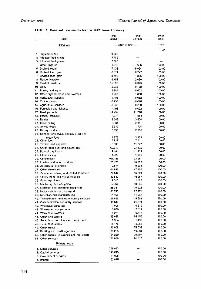
The base solution for the quadratic input-output model developed in this study ispresented in Table 1. The output, primaryinput and final demand levels reported hereare identical to the values reported in the1972 Texas transactions table since the priceindices for all the primary inputs and prod-ucts were equal to 100. The value of theobjective function, or the sum of producerand consumer surplus for all participants inthe Texas economy, was $15,005 billion.Since all prices were indexed, this solutionvalue does not represent an absolute mea-sure of the nominal gain in economic well-being realized by the participants in the 1972

Texas economy. This solution value, howev-er, does provide the basis against which thesolution values associated with a cutback inagricultural production can be compared.

The value of the producer and consumersurpluses reported in Table 4 for selectedagriculturally-related sectors must also beinterpreted the same way. Note producersurplus is smaller than consumer surplus.This can be explained by the relatively highelasticities used in formulating the primaryinput supply functions in this study.

Effects of a Cutback inAgricultural Production

There are a variety of potential capacity-related issues that could be addressed withthe model developed in this study. Becausethe sectors producing agricultural productsboth supply and receive production inputsfrom other production sectors, the actions ofagricultural producers will affect the outputof other production sectors, and vice-versa.Our interest in this paper is to determine theeffect that a cutback in agricultural produc-tion would have had on the utilization ofcapacity in other production sectors as well asthe economic well-being of all the partici-pants in the 1972 Texas economy.

Design of Simulations

Let us assume that Texas crop and live-stock producers in 1972 had cut back theirproduction plans by 35 percent of the outputlevels reported in Table 1. Due to thebiological nature of agricultural productionprocesses, once a crop has not been plantedor breeding livestock have not been bred,the resulting production levels in effect rep-resent the current engineering capacities ofthese sectors. The engineering capacities ofthe agricultural production sectors thereforewere set at 65 percent of the actual outputproduced in 1972. From a programmingstandpoint, this required substituting theseengineering capacities into the Mx matrix inequation (10). Given the assumption of a 35

113

Penson and Fulton

Western Journal of Agricultural Economics

TABLE 1. Base solution results for the 1972 Texas Economy.

Total FinalSector output demand

Products

1. Irrigated cotton2. Irrigated food grains3. Irrigated feed grains4. Other irrigated5. Dryland cotton6. Dryland food grain7. Dryland feed grain8. Range livestock9. Feedlot livestock

10. Dairy11. Poultry and eggs12. Other dryland crops and livestock13. Agricultural supplies14. Cotton ginning15. Agricultural services16. Forestries and fisheries17. Meat products18. Poultry products19. Dairies20. Grain milling21. Animal feeds22. Bakery products23. Canned, preserved, pickled, dried and

frozen food24. Other food25. Textiles and apparels26. Crude petroleum and natural gas27. Natural gas liquids28. Other mining29. Construction30. Lumber and wood products31. Agricultural chemicals32. Other chemicals33. Petroleum refining and related industries34. Glass, stone and metal products35. Farm machinery36. Machinery and equipment37. Electrical and electronic equipment38. Motor vehicles and transport39. Miscellaneous manufacturing40. Transportation and warehousing services41. Communication and utility services42. Wholesale groceries43. Wholesale crop products44. Wholesale livestock45. Other wholesaling46. Retail farm machinery and equipment47. Retail food stores48. Other Retail49. Banking and credit agencies50. Other finance, insurance and real estate51. Other services

1.

2.

3.

4.

Primary inputs

Labor servicesCapital servicesGovernment servicesImports

- $100 million -

0.738

2.256

2.006

1.949

7.433

0.374

3.482

9.151

15.305

2.933

2.284

1.902

1.708

0.933

3.387

1.496

14.299

1.877

4.642

3.961

3.928

3.195

4.97318.919

13.039

60.717

19.184

11.026

101.186

28.178

2.574

64.896

74.042

49.843

2.316

12.394

25.351

30.795

14.198

36.835

45.647

7.606

3.836

1.261

65.695

1.954

15.476

82.809

35.253

64.259

131.658

359.083

149.615

61.028

162.915

.696

6.924

0.727

1.376

2.030

6.975

0.162

0.602

1.058

0.052

0.070

0.208

0.092

11.778

1.814

3.606

2.951

1.700

2.595

3.35817.011

11.777

23.132

11.139

1.996

93.261

10.658

0.204

47.307

56.221

16.064

1.623

10.266

19.926

27.778

11.654

18.681

21.071

6.619

2.514

0.516

52.455

1.499

15.266

74.538

19.581

29.997

81.113

Priceindex

1972

=100

100.00

100.00

100.00

100.00

100.00

100.00

100.00

100.00

100.00

100.00

100.00

100.00

100.00

100.00

100.00

100.00

100.00

100.00

100.00

100.00100.00

100.00

100.00100.00

100.00

100.00

100.00

100.00

100.00

100.00

100.00

100.00

100.00

100.00

100.00

100.00

100.00

100.00

100.00

100.00

100.00

100.00

100.00

100.00

100.00

100.00

100.00

100.00

114

100.00

100.00

100.00

100.00

December 1980

Impact of Production Cutbacks

percent cutback in agricultural production,the constraints inserted into equation (10)represented 65 percent of the output levelsreported for these sectors in Table 1.

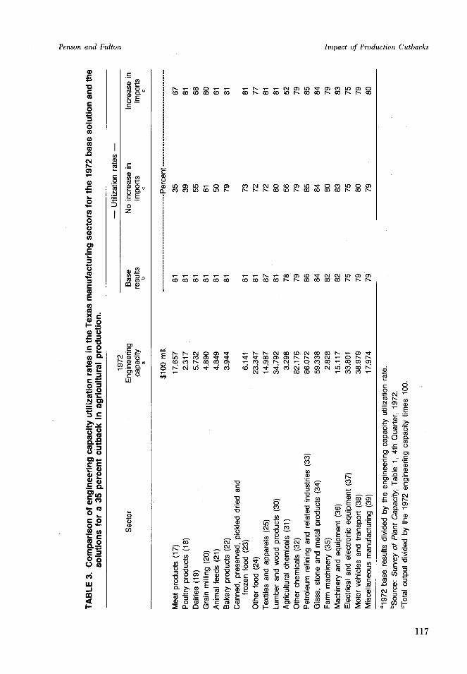
U.S. Department of Commerce surveyresults show the non-agricultural productionsectors in Texas were operating well belowtheir 1972 engineering capacities (see Table3). Thus, their engineering capacities wouldnot have effectively constrained the model'ssolution for the simulations conducted in thispaper and therefore were not entered in theMx matrix.

The effects of a cutback in agriculturalproduction are examined in the following twosimulations. The first simulation assumesprocessors of Texas raw agricultural productscould not increase their imports of theseproducts from other geographical areas. Thesecond simulation relaxes this assumption byexamining what would have happened ifthese processors imported 50 percent of theiragricultural input needs.

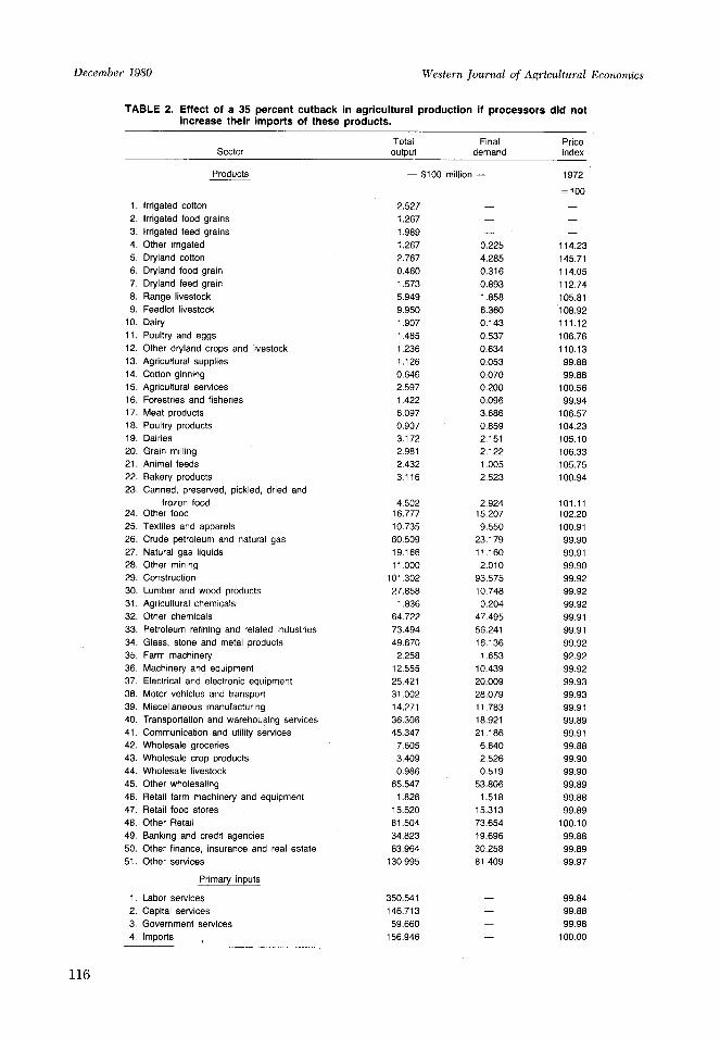
Effects If ImportsNot Increased

The 1972 output, primary input, finaldemand and price levels associated with a 35percent cutback in agricultural production ifprocessors of these products could not in-crease their imports of raw agricultural prod-ucts are reported in Table 2. While therewould have been a substantial increase in theprices agricultural producers receive for mostof their products, not all prices would haveincreased by the same percentage. This isbecause of the different elasticities of de-mand for each product, For example, thecotton production sectors were in a veryinelastic portion of their demand curve andtherefore realized a relatively large percen-tage increase in prices.

The interdependencies within the foodand fiber system in Texas are also evident inthese results. By "bottlenecking" the flow ofraw agricultural products to processors ofthese products, the agricultural productionsectors would have been the capacity limitingproduction sectors in the Texas economy.

For example, when the output of the live-stock production sectors was cut back, there-by causing livestock prices to rise anywherefrom 6 to 12 percent, the output of livestockprocessors would have declined as well. This,in turn, would also have caused the prices ofprocessed foods to increase. Those manufac-turing sectors not directly related to agricul-ture would have been relatively unaffectedby the cutback in agricultural production,however.

We can further illustrate the short-runeffects of this cutback in agricultural produc-tion on the manufacturing sectors by examin-ing their engineering capacity utilizationrates. Looking at these rates both before andafter the cutback in agricultural production inTable 3, we see those non-agricultural pro-duction sectors hardest hit by the cutbackwould have been those who utilize rawagricultural products as an input to theirproduction processes. For example, the engi-neering capacity utilization rates in the meatproducts, poultry products, dairies and ani-mal feeds sectors would have been fallensharply if agricultural production were cutback 35 percent. On the other hand, theengineering capacity utilization rate in suchsectors as the glass, stone and metal productssector would have remained unchanged inthe short-run.

The quantity of primary inputs used in theeconomy would have also declined from thelevels reported in the base solution. Becauseless output would have been produced, lessinputs would have been needed and theirprices would have declined. A similar resultwould have occurred for some of the inter-mediate products used by agricultural pro-ducers, such as agricultural supplies, agricul-tural services, fertilizer, farm machinery, andbanking and credit agencies. Total output ofthese sectors would have decreased as less oftheir product would have been demanded bythe agricultural production sectors. The finaldemand for the goods and services suppliedby these and other sectors would havechanged very little, however. Total wagespaid to households in the Texas economy

115

Penson and Fulton

Western Journal of Agricultural Economics

TABLE 2. Effect of a 35 percent cutback in agricultural production if processors did notincrease their imports of these products.

Total Final PriceSector output demand index

Products - $100 million - 1972

=100

1. Irrigated cotton 2.527- -2. Irrigated food grains 1.267-3. Irrigated feed grains 1.989- -4. Other irrigated 1.267 0.225 114.235. Dryland cotton 2.767 4.285 145.716. Dryland food grain 0.460 0.316 114.057. Dryland feed grain 1.573 0.893 112.748. Range livestock 5.949 1.858 105.819. Feedlot livestock 9.950 6.360 108.92

10. Dairy 1.907 0.143 111.1211. Poultry and eggs 1.485 0.537 106.7612. Other dryland crops and livestock 1.236 0.634 110.1313. Agricultural supplies 1.126 0.053 99.8814. Cotton ginning 0.646 0.070 99.8815. Agricultural services 2.597 0.200 100.5616. Forestries and fisheries 1.422 0.096 99.9417. Meat products 6.097 3.686 106.5718. Poultry products 0.907 0.859 104.2319. Dairies 3.172 2.151 105.1020. Grain milling 2.981 2.122 106.3321. Animal feeds 2.432 1.005 105.7522. Bakery products 3.116 2.523 100.9423. Canned, preserved, pickled, dried and

frozen food 4.502 2.924 101.1124. Other food 16.777 15.207 102.2025. Textiles and apparels 10.735 9.550 100.9126. Crude petroleum and natural gas 60.509 23.179 99.9027. Natural gas liquids 19.166 11.160 99.9128. Other mining 11.000 2.010 99.9029. Construction 101.302 93.575 99.9230. Lumber and wood products 27.858 10.748 99.9231. Agricultural chemicals 1.836 0.204 99.9232. Other chemicals 64.722 47.495 99.9133. Petroleum refining and related industries 73.494 56.241 99.9134. Glass, stone and metal products 49.670 16.136 99.9235. Farm machinery 2.258 1.653 92.9236. Machinery and equipment 12.555 10.439 99.9237. Electrical and electronic equipment 25.421 20.009 99.9338. Motor vehicles and transport 31.002 28.079 99.9339. Miscellaneous manufacturing 14.271 11.783 99.9140. Transportation and warehousing services 36.306 18.921 99.8941. Communication and utility services 45.347 21.186 99.9142. Wholesale groceries 7.605 6.640 99.8843. Wholesale crop products 3.409 2.526 99.9044. Wholesale livestock 0.986 0.519 99.9045. Other wholesaling 65.547 53.806 99.8946. Retail farm machinery and equipment 1.826 1.518 99.8847. Retail food stores 15.520 15.313 99.8948. Other Retail 81.504 73.654 100.1049. Banking and credit agencies 34.823 19.696 99.8850. Other finance, insurance and real estate 63.964 30.258 99.8951. Other services 130.995 81.409 99.97

Primary inputs

1. Labor services 350.541 - 99.842. Capital services 146.713 - 99.883. Government services 59.660 -99.984. Imports 156.946 - 100.00

116

December 1980

Penson and Fulton

C)

0

._

cm

0

o

0)

a)0)

_

Os0

c)

0)

C

._ac

L.o

0)

Q-0

o

w

ca)'

a)

.Cn

O

I-"

a)

3oN

c

) c

0

Cmo

C

a)

0.

a)'

0)

cn a) CZ) c C

w

C)

U)

C6

C. 00 D0 C: 0 0 0

COCOCO C

D) LO C) LO -00) C1)

CO) C) LO CD LOC -

o0 o o 0 co 0 0 0

LO -T- O~ C1 CO '4 'I t

co ~ Cu o otCM

CO U~~~~~)

*0

t5 C) l) ) C

a)C)

'a CLVcJ

L- E N

a)o ~Cc$ Ca~o. QO< cno

a_ 0 (D < m

0 0- N 0 0 c M M 0 M 0N CO O ) LO O O CO r- No O

.N 0 U) 0 C O Cc N LO 0

O O cO w N CO CO CO O N N N

N N C 0 C Cm O CNO Not -0C 0 -o aO ) N N C co - C o Nr

CVo 0) N C 0 CO CO - CO) C0 )cm co ~~~0 0SCN

CY)CO

CO'n

- - Co=

vm)

ao0 Q CM0 - C CZ c

c C -o

£" ( .) a) C ) )

S) ro O U

-r X E - Ca) 0)

0 I-i< 0 O.

-IIf-C

CD b t 0)

E0 c2 S1) o 0.E'E cm

a) C ) ) Ca

E E:

£ 2 a)02

Impact of Production Cutbacks

C

C\

.N C0 a)

E

C Ia a .)a

(,!,

)- CM

£ QD l

_ *a)

a) a)

(0 0)

(0 .._

C) 0 0D! CDCl !

117

Western Journal of Agricultural Economics

would have fallen by 2.4 percent to $350.5billion while indirect business taxes wouldhave fallen by $1.4 billion, a 2.2 percentdecline.

As one might expect, the total value ofproducer and consumer surplus in the Texaseconomy would have declined as a result ofthe cutback in agricultural production. Whilethe total gain in economic well-being realizedby participants in the economy would havebeen less than if there were no cutback inagricultural production, agricultural produc-ers would have been better-off economically.Producer surplus in the agricultural produc-tion sectors would have increased by $417.4billion. The results presented in Table 4indicate this gain would have been achievedlargely at the expense of consumers, whosegain in economic well-being from purchasingTexas products would have declined by 40percent. Producers in the agriculturally-related sectors would have suffered a 33percent decline in producer surplus. Thus,the gain in economic well-being achieved byagricultural producers was not large enoughto offset the lower producer and consumersurpluses for other participants in the Texaseconomy. If agricultural producers in futureperiods were to respond to these higherproduct prices by no longer cutting backtheir production, however, the prices andproducer and consumer surpluses reportedhere would return to the levels reported inthe base solution.

Effects If Imports Increased

Let us now assume that the processors ofraw agricultural products in Texas, in re-sponse to the announced cutbacks by agricul-tural producers, contracted for 50 percent oftheir needs for these inputs with producersoutside Texas. The output, final demand,primary input and price levels associatedwith this simulation are reported in Table 5.A review of this table shows the output ofsome agricultural production sectors wouldhave been reduced due to the lower totaldemand for their product. Others, like the

118

cotton production sectors, would not havehad to cut back their output since the totaldemand for their product still exceeded theirengineering capacities. The prices receivedby all agricultural producers, however,would have been lower than those reportedin Table 2, where processors of raw agricul-tural products could not increase their im-ports of these products. The output of Texasprocessors of raw agricultural products inTable 5 would have been higher as well. Forexample, the meat products sector wouldnow have been producing $11.824 billion inprocessed meats as compared to the $6.097billion figure reported in Table 2. This is stillconsiderably less than the $14.299 billionfigure reported before the cutback in agricul-tural production in Table 1. The prices forprocessed foods also would have fallen fromthe values reported in Table 2, whereprocessors could not increase their imports ofraw agricultural products. The index of pricespaid for meat products, for example, wouldhave fallen back to 101.99, still slightly abovethe price index of 100 before the cutback inagricultural production but substantially be-low the index of 106.57 reported in Table 2.Total wages paid to households and indirectbusiness taxes would have also increasedfrom the values reported in Table 2, butthese payments would have still been muchlower than the values received before thecutback in agricultural production.

A comparison of the engineering capacityutilization rates for the agriculturally-relatedproduction sectors in Table 3 shows that mostof these sectors would now have been opera-ting at higher utilization rates, althoughthese rates would have still been lower thanthose reported before the cutback in agricul-tural production. Note that some of thesesectors would have been operating below thecapacity utilization rates found whenprocessors of raw agricultural products couldnot increase their imports of these products.For example, the farm machinery and ag-ricultural chemicals sectors would have beenoperating at 79 and 52 percent of theircapacities, respectively. This would have

December 1980

Penson and Fulton Impact of Production Cutbacks

LnCMC\i

0)a

COCi

CM

o 't it 0 N U N07 O s O r 0

0 CO C - 0a) - COCM D 0

CY)

T) 0T CM Ot n 0t -

r-

CD T

r- N

LnCO

t O N e) 0 ) Cs Sd c u6 r cCE ci csi c'tf LCO C 40 CM C', - t

.rD

0 00t

0CE)

't s- CMN N- C T-O Nr CD -0 O 0

d d od cD<5 r.t..- O a) -

04

CO T-- 0) tC 'ol0 CO U) lO CM 0 t ( -

)O CM 't '- CE) VOCM

o0 0) CM 0 - OC Co C) C) o) CD O - C

N CM CO LItU CO)

O CM U) o- CE 0LO) O C 0 CO CE) 0t COai cui ci LO C) o

N-

CO)CO

C

,D rf ,~.+ +CM

U) -+ CD CVO0in r- ^^^

CO 0 CMN N- CO NN CD CO CO CO CMd ci u L6 cL Lo

O CD- r 0a) N

LO'0 ON- oCM

04CO

CM0COCD'U

0CM

0)

L0

COCf

LL 0O

C0 )0

C)

U1) 00 70 ~ ~ =

L) LU

(0 UCc

COa

J) 0 CY) -id

CUCC L)

> 0)~VV -0 -CY -

00000L1.0a- O 0)

0 -i, (1CO,

co CIO as CY) L1

co 0~o~0 a: LL a.~

t- CE) T- N o0 co- 0) N- N -O CY)N-_ -I NiCM O

CM) 0) 00 T-NCO CM N CM -Cd N CM Co) - CiL) CV CIO T- 't

't r CM 1N CMt4 - 7- r t (D

4 t od CD Coi LCM

0) V- 0 -0) CO 0t 't CO a) CD O CO)'- C O N COD E)

r- CD C CM co CO

C)0C

0C C4

ciCO6N p

14t 0 T-Lo"'

L6 0 CT-

0C0 CMN c)o a o6 t-O t -- C0T-C-CM

0CEi

00 0CON-CO1:

cu SC0

N' oN- 0CONu

- Co CM a) 0 0- CO COCO CO COCM- CD

'It 0) i-0) N- 0CE) CD CE) 00 O CO

v N CVl CVl C*»- 1'MCM CM'-N-NN

r O t C CMM19 (CD t d O(0 CE rN-O CE)

NCD t

CON-

CE0

o0

C\i

CO

CO

0

Cj

CO

r-

-c

-0

-o - o

c co §p C iNONa oc CM0 O C

a LC

0- 0) NCq 0 2 02

^^ a f ^ (3 .4s 1-y- I-

|) 6 CU E CU CU a) 0) CU

119

IDm -w E| iiC

cn:3

a-

CO

L-

a):3-o00.

co0u

EC:

a)

0oc

co

0

EC

u)co

C.

0z

Cu

U3CD

-I

c

a)

0

0in

(U

co

COL.

0me-

I)

0

.2'o

c

-

0)

nO

Q)

c_0

C)

,4

I

O

11a).

-I

LU

I-1

Eu,

O0

0a) c

oU)0

c)l

a-"

0 3O co

0:_ao

cn

cn0'40

a.

U)

C0

3

L

I

c

IE

)

II

_ _ _ _ _ _ _ _ _ _~~~ I

Western Journal of Agricultural Economics

TABLE 5. Effect of a 35 percent cutback in agricultural production if processors imported 50percent of their agricultural input needs.

Total Final PriceSector output demand index

Products - $100 million - 1972

=100

1. Irrigated cotton 2.527 - -2. Irrigated food grains 1.267-3. Irrigated feed grains 1.989 -4. Other irrigated crops 1.267 0.690 100.275. Dryland cotton 2.767 4.715 138.216. Dryland food grain 0.379 0.730 99.907. Dryland feed grain 0.815 1.379 99.178. Range livestock 4.568 2.032 100.119. Feedlot livestock 9.950 6.499 106.46

10. Dairy 1.467 0.162 100.1511. Poultry and eggs 1.417 0.601 100.1812. Other dryland crops and livestock 1.236 0.952 102.5313. Agricultural supplies 1.034 0.052 99.9814. Cotton ginning 0.646 0.070 99.8515. Agricultural services 2.457 0.209 99.9516. Forestries and fisheries 1.503 0.097 99.9317. Meat products 11.824 9.334 101.9918. Poultry products 1.866 1.806 100.0319. Dairies 4.644 3.607 99.9920. Grain milling 3.895 2.959 99.9421. Animal feeds 2.980 1.627 100.7222. Bakery products 3.199 2.598 99.9723. Canned, preserved, pickled, dried and

frozen food 4.993 3.376 99.9624. Other food 18.001 16.409 100.7425. Textiles and apparels 12.167 10.930 100.3526. Crude petroleum and natural gas 60.683 23.171 99.9227. Natural gas liquids 19.164 11.156 99.9228. Other mining 11.015 2.009 99.9029. Construction 101.318 93.581 99.9230. Lumber and wood products 28.112 10.750 99.9231. Agricultural chemicals 1.717 0.204 99.9132. Other chemicals 64.747 47.536 99.8933. Petroleum refining and related industries 73.433 56.241 99.9134. Glass, stone and metal products 49.819 16.144 99.9135. Farm machinery 2.237 1.650 99.9336. Machinery and equipment 12.549 10.424 99.9237. Electrical and electronic equipment 25.429 20.002 99.9338. Motor vehicles and transport 30.972 28.047 99.9439. Miscellaneous manufacturing 14.313 11.783 99.9140. Transportation and warehousing services 36.536 18.932 99.8941. Communication and utility services 46.433 22.028 99.2042. Wholesale groceries 7.624 6.639 99.8943. Wholesale crop products 3.383 2.526 99.9144. Wholesale livestock 0.980 0.520 99.9145. Other wholesaling 66.511 53.737 99.8946. Retail farm machinery and equipment 1.794 1.518 99.8947. Retail food stores 15.525 15.315 99.8848. Other Retail 82.904 75.077 99.9449. Banking and credit agencies 34.509 19.683 100.2250. Other finance, insurance and real estate 64.205 30.291 99.8751. Other services 132.047 82.106 99.90

Primary inputs

1. Labor services 352.440 -99.882. Capital services 147.880 - 99.933. Government services 60.242 - 99.994. Imports 171.054 - 100.00

120

December 1980

Impact of Production Cutbacks

been caused by the reduced input needs ofthe agricultural production sectors becauseprocessors of raw agricultural products im-ported part of their input needs from othergeographical areas.

Finally, a review of Table 4 shows consum-ers would have been economically better-offif Texas processors of raw agricultural prod-ucts could have increased their imports toavoid a disruption to their production plans.Yet, consumers still would not have been aswell-off economically as they would havebeen had agricultural producers not cut backtheir production. This was also true of theeconomic well-being of producers in all theagriculturally-related production sectors ex-cept the farm machinery production sector.All agricultural producers except those inthe feedlot livestock production sector wouldnow have been worse-off economically thanthey would have been if the processors of rawagricultural products could not increase theirimports of these products. Importantly, someof these producers would now have beenworse-off economically than they were beforethey cut back their production. This occurredto the producers of food and feed grains, forexample. This helps underscore the risksagricultural producers undertake by cuttingback their production. This loss is economicwell-being could have been even greater ifTexas processors had increased their importsof these products even further. Why wouldfeedlot livestock producers be better-off eco-nomically if processors increased their im-ports of raw agricultural products? Whiletheir gross revenue would have been lower,feedlot livestock producers would have bene-fited from lower costs of feeder calves andfeed grains. Thus, while their quasi-economic rent would have been lower underthis scenario, feedlot livestock producers'economic rent would have been substantiallyhigher.

Concluding Remarks

The allowance for sector engineeringcapacities in a quadratic input-output model

for a state economy allows one to identify theeffects that localized cutbacks in agriculturalproduction would have upon producers andconsumers throughout the economy. Using aquadratic input-output model developed forthe 1972 Texas economy, we showed a cut-back in production by agricultural producerswould increase their economic well-being ifprocessors of raw agricultural products couldnot increase their imports of these products.However, the economic well-being of con-sumers and other producers in the Texaseconomy would have been less than it wasbefore the cutback. If Texas processors of rawagricultural products could have increasedtheir imports of these products from othergeographical areas, however, the cutback byagricultural producers could backfire onthem as illustrated in this study. The excep-tion to this conclusion was feedlot livestockproducers, who would benefit from the lowercosts they would have to pay for feeder calvesand feed grain.

References

Almon, Clopper, Jr., The American Economy to 1975,New York, Harper and Row, 1966.

Dorfman, Robert, Paul A. Samuelson, and Robert M.Solow, Linear Programming and Economic Analysis,New York, McGraw-Hill, 1958.

Fulton, Murray E., "The Capacity of the Food and FibreSystem and Its Interface with the General Economy:An Application of a Quadratic Input-Output Model forthe Texas Economy", unpublished M.S. thesis, De-partment of Agricultural Economics, Texas A&MUniversity, 1978.

George, P. S., and G. A. King, Consumer Demand forFood Commodities in the United States with Projec-tions for 1980, Gianinni Foundation Monograph No.26, March 1971.

Grubb, Herbert W., Texas Input-Output Model, 1972,Planning and Development Division, Texas Depart-ment of Water Resources, February 1978.

121

Penson and Fulton

Western Journal of Agricultural Economics

Harrington, David H., "Quadratic Input-Output Analy-sis: Methodology for Empirical General EquilibriumModels", Ph.D. thesis, Department of AgriculturalEconomics, Purdue University, 1973.

Houthakker, H. S., and L. D. Taylor, Consumer De-mand in the United States, Analysis and Projections,2nd edition, Cambridge, Massachusetts, HarvardUniversity Press, 1970.

Kinoshita, Richard K., Basic Economic Indicators, Cur-rent Fisheries Statistics No. 6131, U.S. Dept. ofCommerce, Washington, D.C., June 1973.

Leontief, Wassily W., The Structure of AmericanEconomy, 1919-1939, 2nd edition, New York, OxfordUniversity Press, 1951.

Penson, John B., Jr., and Murray E. Fulton, Descrip-tion and Use of a Quadratic Input-Output Model forthe Texas Economy, Departmental Technical ReportNo. DTR 79-5, Texas Agricultural Experiment Sta-tion, 1979.

Plessner, Yakir, "Activity Analysis, Quadratic Pro-gramming and General Equilibrium", Int. Econ.Rev., 8(1967): 168-179.

Ray, Daryll E., and James W. Richardson, DetailedDescription of POLYSIM, Technical Bulletin T-151,Oklahoma Experiment Station, 1978.

Speilmann, Heinz, and Eldon E. Weeks, "Inventoryand Critique of Estimates of U.S. Agricultural Capaci-ty", Amer. J. Agr. Econ., 57(1975): 921-928.

U.S. Department of Commerce, Survey of Plant Capac-ity, 1973, Current Industrial Reports Series MQ-CL(73-1), Washington, D.C., 1975.

Wilson, Robert R., "Petroleum for U.S. Agriculture",Amer. J. Agr. Econ., 56(1974): 888-895.

122

December 1980