IEEE TRANSACTIONS ON MEDICAL IMAGING, VOL. 26, NO. 12 ...

IEEE TRANSACTIONS ON MEDICAL IMAGING, VOL. 26, NO. 12, DECEMBER 2007 1681

A Reconstruction Method for Gappy andNoisy Arterial Flow Data

Alexander Yakhot*, Tomer Anor, and George Em Karniadakis

Abstract—Proper orthogonal decomposition (POD), Kriginginterpolation, and smoothing are applied to reconstruct gappyand noisy data of blood flow in a carotid artery. While we haveapplied these techniques to clinical data, in this paper in order torigorously evaluate their effectiveness we rely on data obtainedby computational fluid dynamics (CFD). Specifically, gappy datasets are generated by removing nodal values from high-resolution3-D CFD data (at random or in a fixed area) while noisy data setsare formed by superimposing speckle noise on the CFD results.A combined POD-Kriging procedure is applied to planar datasets mimicking coarse resolution “ultrasound-like” blood flowimages. A method for locating the vessel wall boundary and forcalculating the wall shear stress (WSS) is also proposed. Theresults show good agreement with the original CFD data. Thecombined POD-Kriging method, enhanced by proper smoothingif needed, holds great potential in dealing effectively with gappyand noisy data reconstruction of in vivo velocity measurementsbased on color Doppler ultrasound (CDUS) imaging or magneticresonance angiography (MRA).

Index Terms—Carotid artery, computational fluid dynamics(CFD), kriging interpolation, proper orthogonal decomposition.

I. INTRODUCTION

THE RECENT advances in medical imaging have generateda lot of interest in developing in vivo techniques to obtain

quantitative data for blood flow in arteries. Color Doppler ul-trasound (CDUS) imaging is very effective in obtaining mapsrepresenting blood flow characteristics based on the Dopplerprinciple. Magnetic resonance phase contrast (MR PC) velocitymapping methods encode the motion of flowing blood into thephase of the acquired signal. At the present time, there are stillserious limitations in the spatial or temporal resolution of mag-netic resonance imaging (MRI) and CDUS imaging. MRI is a3-D technique for velocity imaging with high spatial resolutionbut low temporal resolution. Furthermore, it suffers from signalloss in turbulent flow, thus making it ineffective in imaging

Manuscript received January 23, 2007; revised May 15, 2007. This workwas supported in part by the National Science Foundation under Grant IMAGand Grant CI-TEAM and in part by the United States–Israel Binational ScienceFoundation under Grant 2001-150. Asterisk indicates corresponding author.

*A. Yakhot is with the Department of Mechanical Engineering, Ben-GurionUniversity of the Negev, Beersheva 84105, Israel (e-mail: [email protected]).

T. Anor was with the Department of Mechanical Engineering, Ben-GurionUniversity of the Negev, Beersheva 84105, Israel. He is currently with the Neu-rosurgery Department, Children’s Hospital Boston, Harvard Medical School,Boston, MA 02115 USA.

G. Em Karniadakis is with the Division of Applied Mathematics, Brown Uni-versity, Providence, RI 02912 USA.

Color versions of some of the figures in this paper are available online athttp://ieeexplore.ieee.org.

Digital Object Identifier 10.1109/TMI.2007.901991

stenotic arteries. CDUS imaging has very good temporal reso-lution but in conventional commercial ultrasound systems onlythe axial component of flow velocity can be estimated and visu-alized using the classic Doppler effect. To extend flow velocityestimation to two or three components, a number of techniqueshave been proposed [4], [5], [7], [11] but such systems requiretwo or more transducers. However, the temporal resolution maybe reduced by the occurrence of gappy regions if, for example,the imaged artery lies behind a bony structure. Several artifactsalso occur during medical scanning, which may increase uncer-tainty in the data processing and lead to erroneous interpreta-tions. Hence, part of the data may be discarded at some time in-stants due to being outside a prespecified confidence threshold.This may lead to spatial-temporal gappiness or, in some cases,part of the information may be totally missing due to shadowing(i.e., obstructed view), leading to the so-called “black zones.”

More specifically, the effects of artifacts in MR PC velocityimaging were considered in [29]. The authors studied caseswhen velocity displacement artifacts may register incorrectvelocities to correct spatial locations. Spatial displacementartifacts may lead to a distortion of the lumen and velocitiesassigning the correct velocity field to incorrect spatial locations.Also, noise of different types and sources contaminates medicalultrasound (US) and MR imaging. For example, a US imageis generated by reflected coherent ultrasound waves at fixedfrequencies that interact with different tissue types and giverise to various interface phenomena causing speckle noise. Inpractice, speckle type is the dominant source of noise in USthat should be filtered out [27].

Magnetic resonance angiography (MRA) is widely used fornoninvasive and accurate acquisition of 3-D arterial geometries.Recently, a new technique, 3-D US was tested as an alterna-tive to MRA for generating anatomically realistic 3-D geometricmodels [3]. The geometric model data is then exported intocomputational fluid dynamics (CFD) codes to obtain detaileddescription of the blood velocity field [23], [24], [26], [30].It is believed that accurate CFD simulation of the blood flowcan yield reliable quantification of the vessel wall shear stress(WSS), which plays a critical role in regulating the arterial struc-ture [8], [12], [19]. Errors in image segmentation might affectCFD-based prediction of WSS. In [24], the authors consideredthe case of a straight cylindrical tube and performed CFD sim-ulations based on a geometrical model obtained from magneticresonance imaging (MRI). The computed WSS had errors upto 40%, however, a simple smoothing of the image boundarydata reduced the errors to less than 16%. Time-resolved directmeasurements of WSS remains a great challenge despite iso-lated successes using MRI or Doppler US methods (see [18],[25], [26], [31], [32], [35] and [2], [6], [14], respectively). Most

0278-0062/$25.00 © 2007 IEEE

1682 IEEE TRANSACTIONS ON MEDICAL IMAGING, VOL. 26, NO. 12, DECEMBER 2007

of these measurements have been restricted to the axial velocitycomponent in a single plane or even in a single location. In [35],WSS derived from the 3-D MR PC velocity mapping measure-ments did not differ from the 2-D velocity measurements bothin vivo or in vitro. Accurate estimation of WSS vectors requiresaccurate measurement of the near-wall velocity vector field andaccurate identification of the vessel wall location. In [18], thenear-wall velocity velocity field was fitted by high-order poly-nomials in order to reduce the experimental data noise. Thespatial derivatives of the fitted velocity yielded WSS while thevessel boundaries were obtained from the geometric model.

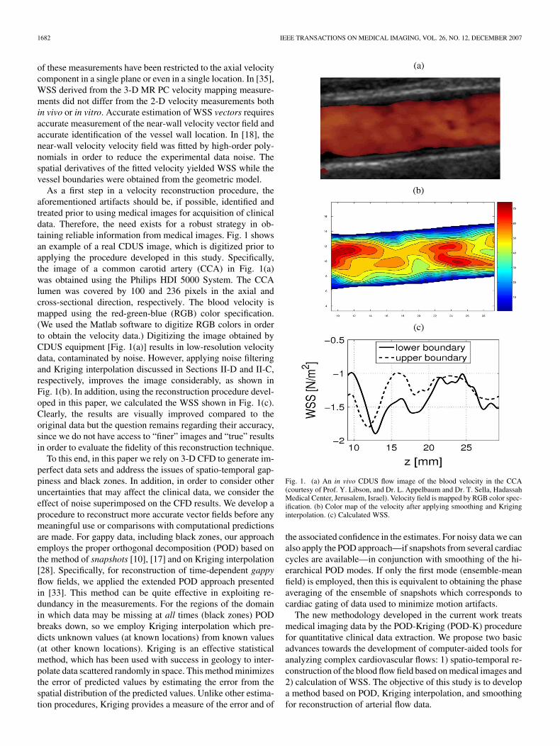
As a first step in a velocity reconstruction procedure, theaforementioned artifacts should be, if possible, identified andtreated prior to using medical images for acquisition of clinicaldata. Therefore, the need exists for a robust strategy in ob-taining reliable information from medical images. Fig. 1 showsan example of a real CDUS image, which is digitized prior toapplying the procedure developed in this study. Specifically,the image of a common carotid artery (CCA) in Fig. 1(a)was obtained using the Philips HDI 5000 System. The CCAlumen was covered by 100 and 236 pixels in the axial andcross-sectional direction, respectively. The blood velocity ismapped using the red-green-blue (RGB) color specification.(We used the Matlab software to digitize RGB colors in orderto obtain the velocity data.) Digitizing the image obtained byCDUS equipment [Fig. 1(a)] results in low-resolution velocitydata, contaminated by noise. However, applying noise filteringand Kriging interpolation discussed in Sections II-D and II-C,respectively, improves the image considerably, as shown inFig. 1(b). In addition, using the reconstruction procedure devel-oped in this paper, we calculated the WSS shown in Fig. 1(c).Clearly, the results are visually improved compared to theoriginal data but the question remains regarding their accuracy,since we do not have access to “finer” images and “true” resultsin order to evaluate the fidelity of this reconstruction technique.

To this end, in this paper we rely on 3-D CFD to generate im-perfect data sets and address the issues of spatio-temporal gap-piness and black zones. In addition, in order to consider otheruncertainties that may affect the clinical data, we consider theeffect of noise superimposed on the CFD results. We develop aprocedure to reconstruct more accurate vector fields before anymeaningful use or comparisons with computational predictionsare made. For gappy data, including black zones, our approachemploys the proper orthogonal decomposition (POD) based onthe method of snapshots [10], [17] and on Kriging interpolation[28]. Specifically, for reconstruction of time-dependent gappyflow fields, we applied the extended POD approach presentedin [33]. This method can be quite effective in exploiting re-dundancy in the measurements. For the regions of the domainin which data may be missing at all times (black zones) PODbreaks down, so we employ Kriging interpolation which pre-dicts unknown values (at known locations) from known values(at other known locations). Kriging is an effective statisticalmethod, which has been used with success in geology to inter-polate data scattered randomly in space. This method minimizesthe error of predicted values by estimating the error from thespatial distribution of the predicted values. Unlike other estima-tion procedures, Kriging provides a measure of the error and of

Fig. 1. (a) An in vivo CDUS flow image of the blood velocity in the CCA(courtesy of Prof. Y. Libson, and Dr. L. Appelbaum and Dr. T. Sella, HadassahMedical Center, Jerusalem, Israel). Velocity field is mapped by RGB color spec-ification. (b) Color map of the velocity after applying smoothing and Kriginginterpolation. (c) Calculated WSS.

the associated confidence in the estimates. For noisy data we canalso apply the POD approach—if snapshots from several cardiaccycles are available—in conjunction with smoothing of the hi-erarchical POD modes. If only the first mode (ensemble-meanfield) is employed, then this is equivalent to obtaining the phaseaveraging of the ensemble of snapshots which corresponds tocardiac gating of data used to minimize motion artifacts.

The new methodology developed in the current work treatsmedical imaging data by the POD-Kriging (POD-K) procedurefor quantitative clinical data extraction. We propose two basicadvances towards the development of computer-aided tools foranalyzing complex cardiovascular flows: 1) spatio-temporal re-construction of the blood flow field based on medical images and2) calculation of WSS. The objective of this study is to developa method based on POD, Kriging interpolation, and smoothingfor reconstruction of arterial flow data.

YAKHOT et al.: A RECONSTRUCTION METHOD FOR GAPPY AND NOISY ARTERIAL FLOW DATA 1683

The paper is organized as follows. The theoretical aspectsof the POD method are outlined in Sections II-A and II-B. InSections II-C and II-D, we describe the Kriging interpolationand smoothing algorithm for noisy data. Formation of clinicaldata prototypes is explained in Section II-E. In Section III, wepresent the results of arterial flow data acquisition from gappydata and data with black zones (Section III-A) and from ultra-sound-like noisy images (Section III-B). In Section IV, we dis-cuss limitations and advantages of the developed method. Fi-nally, in the Appendix we present details on the geometric modeland on the CFD simulation.

II. METHODS

In the next two sections, we present an overview of the POD-based approach for gappy data and outline the Kriging proce-dure for black zones and for subpixel interpolation [13], [20].Subsequently, we discuss smoothing of noisy data, and finallywe describe how we generate clinical data prototypes and ultra-sound-like noisy images from CFD results.

A. Proper Orthogonal Decomposition

We employ the following decomposition of a function

(1)

where , and and are the th orthog-onal spatial and temporal modes, respectively. The POD proce-dure yields the eigenfunctions , which form the expansionbasis in the above expression. Here, we implement the standardmethod of snapshots [10], [17] to obtain eigenfunctions and cor-responding eigenvalues. Consider the collection of data snap-shots, , where is a vector containing the velocityfield at time for all , namely the elements of

are

(2)

These snapshots are used to compute the POD basis vectors,which yield a representation of the data that is optimal in thesense that, for any given basis size, the norm of the error isminimized. This is equivalent to solving the eigenvalue problem

(3)

where the eigenvectors (columns of the matrix A) representthe temporal modes, is a diagonal matrix of the eigenvalues

, and C is a correlation matrix formed by computing the innerproduct between every pair of snapshots and

(4)

The magnitude of the th eigenvalue represents the rela-tive importance of the th POD basis vector. This importanceis commonly quantified by defining the relative energy content

for each basis vector as

(5)

where the term “energy” refers to a measure in the norm.The th POD basis vector, , is given by a linear combinationof snapshots

(6)

where denotes the th element of the th eigenvector .Finally, the reconstruction of the velocity field usingmodes is given by

(7)

for every .

B. Gappy POD

This procedure was developed by Everson and Sirovich in[10] and can be described as follows [13]. The first step is to de-fine a mask vector, which for a particular flow vector describeswhere data are available and where data are missing. For theflow solution , the corresponding mask vector is definedas follows:

(8)

for and . Pointwise multipli-cation is defined as . Then the gappy innerproduct is defined as , and the corre-sponding norm is .

Let be the standard POD basis for the snapshotset , where all snapshots are completely known. Let

be another set of solution vectors that have some ele-ments missing, with corresponding mask vectors . We wantto reconstruct the full or repaired vector from the incompletevectors . Assuming that the vectors representa solution whose behavior can be characterized with the ex-isting snapshot set, the intermediate repaired vectorcan be expressed in terms of POD basis functions as follows:

(9)


To compute the POD coefficients , the error, , between theoriginal and repaired vectors must be minimized. The squarederror is defined as

(10)

using the gappy-norm so that only the original existing data ele-ments in are compared. The coefficients that minimize theerror can be found by differentiating (10) with respect to eachof the in turn. This leads to the linear system of equations

(11)

where

(12)

and

(13)

Solving (11) for and using (9), the intermediate repaired vec-tors can be obtained. Finally, the completeis reconstructed by replacing the missing elements in by thecorresponding repaired elements in , i.e., if .

The initial condition used in the gappy region is typically thenonzero average value over all snapshots. A more robust ver-sion that does not depend on the initial guess and, in addition,enhances accuracy significantly was presented in [33]. The mainsteps of this iterative procedure are as follows.

Iterative Gappy POD (IG-POD):1) Perform Gappy POD but employ only modes in the

reconstruction (9).2) Use the result of the previous step as a new initial guess

at the gappy points and apply Gapy-POD, but now employmodes in the reconstruction.

3) Proceed similarly for the -th iteration until the obtainedeigenspectrum does not change anymore.

In [33], the authors suggest to employ two modesas the starting number of modes. However, in the present study,setting , as suggested in the algorithm above, leads tobetter accuracy.

C. Kriging Interpolation

We have adopted the Kriging interpolation method imple-mented in the Matlab toolbox DACE [20]. Let be composedof known points, i.e., . A knownvalue (response) of a function at those locations is denoted as

. For example, may be one of the three com-ponents of a velocity vector at point . Let be the vectorcontaining all those responses, i.e., . Let

be composed of points x where the value of a function is un-known. The data is arranged in a matrix form and normalized,i.e., the mean of each vector ( th column in a matrix) is zero

Fig. 2. Flow rate versus time. Marked times correspond to instants for whichwe perform the analysis although most results we present are for t = 0:2 s.

and the covariance is equal to unity. For the set of samplingpoints, we define the interpolation matrix as

(14)

where , are polynomial functions. In thisstudy, the regression model is based on the second-order poly-nomials, and for any point x with coordinates we have10 polynomials. We also define the correlation matrix

by , where is the correlation param-eter which is inversely proportional to the correlation length.The choice of correlation function should be based on the un-derlying phenomenon. Here, we restrict our attention to correla-tions which are products of stationary, 1-D correlation kernels,i.e., of the form

(15)

where is a coordinate index. Then, the Kriging interpolationat an unknown point x is

(16)

where is the interpolationmatrix ( for the second-order polynomials regressionmodel), and

(17)

(18)

when

(19)

is the vector of correlations. From (17) and (18), and areand matrices, respectively, obtained from the samplingpoints of .


Fig. 3. (a) Carotid artery obtained from MRA; AA and BB are test sections where results are presented. (b) Black zone on the AA-plane.

We use the following correlation models between two pointsin space .

• Exponential kernel:

(20)

• Spline kernel:

(21)

where and

(22)

The correlation decreases with the distance between points, a larger value for leads to a faster decrease.

D. Smoothing Procedure

We applied smoothing to the temporal and spatial PODmodes obtained from the noisy data after a preprocessingstage whereby ensemble-averaging of the available noisy datais performed. Specifically, we employ a locally weightedsmoothing function, which is based on least squares quadraticpolynomial fitting (LOESS), also known as locally weightedpolynomial regression [9]. At each of the points in the dataset a low-degree polynomial is fit to a subset of the data, withindependent variable values near the point whose response isbeing estimated. The polynomial is fit using weighted leastsquares, giving more weight to points near the point whoseresponse is being estimated and less weight to points furtheraway, i.e.,

(23)

The value of the regression function for the point is then ob-tained by evaluating the local polynomial using the independentvariable values for that data point. The subsets of data used foreach weighted least squares fit in LOESS are determined by anearest neighbors algorithm. A user-specified input to the pro-cedure called the “bandwidth” or “smoothing parameter” de-termines how much data is used to fit each local polynomial.The smoothing parameter, , is a number betweenand 1, with denotes the degree of the local polynomial. Thevalue of is determined by the proportion of data used in eachfit. The subset of data used in each weighted least squares fit iscomprised of the (rounded to the next largest integer) pointswhose independent variables values are closest to the point atwhich the response is being estimated.

E. Formation of Clinical Data Prototypes From CFD Results

In order to have a reference basis for evaluating the accuracyof our method, we have performed 3-D CFD simulations of flowthrough a carotid artery. We used two different CFD codes basedon finite volumes and spectral/hp element methods to verify theaccuracy of the CFD results. The specific steps of the computa-tional procedure are summarized in the Appendix.

1) Gappy Data Sets: The CFD results were used to create asampling set of 101 snapshots for data reconstruction. Spatio-temporal gappiness was generated by randomly removing somenodal data in each snapshot. A measure of the “gappiness per-centage” is defined for each snapshot as the ratio between thenumber of grid points (nodes) where the data is missing to thetotal number of nodes on that snapshot. In this study, the gap-piness percentage is the same for all snapshots. In addition, wediscarded the data from a spatially fixed region in all snapshotsto create a “black zone,” as shown in Fig. 3(a); hereafter we willdenote the black zone as .

2) Ultrasound-Like Noisy Images: Color flow mapping(CFM) represents flow velocities in different colors overlaidon the conventional B-mode (“Brightness”) anatomic images.However, the velocity computed from CFM images may notyield accurate results due to signal contamination with bothrandom and colored noise. Here, we generate a clinical-likeprototype by modifying the CFD results using relatively simple


noise models. 1 Specifically, we assume the noise to be randomand uncorrelated with the clean (noise-free) image. The re-sulting ultrasound-like corrupted image can be described by

(24)

where , and are the corrupted image, denoised image, andthe noise, respectively. In Fig. 16(c), we show an example of anoisy image obtained from the CFD results of a common carotidartery.

In practice, for clinical CDUS images, neither the denoisedimage nor the noise component is available. Here, in orderto generate an ultrasound-like prototype of a clinical image, weconsider the CFD results as the denoised image and we superim-pose on it speckle noise, a special type of noise encountered inultrasound B-mode data [1]. We assume that the speckle noisein (24) has nonzero mean in time but it has zero-mean in spacefor every snapshot, i.e., the resulting noise component is derivedfrom

(25)

where is a Rayleigh random variable having probabilitydensity function

(26)

for and the standard deviation .Our goal is to develop a procedure, subject to certain cri-

teria, for recovering the denoised image from (24) or to con-siderably reduce the noise . To estimate the noise level andevaluate the performance of the denoising procedure, we con-sider the signal-to-noise-ratio (SNR) and noise-to-mean-ratio(NMR). For each snapshot we define

(27)

III. RESULTS

We first present reconstruction results for gappy data andblack zones, and subsequently for noisy data. Hereafter, the axisunits are given in [m] unless otherwise specified. Data anal-ysis includes calculation of the velocity field, wall-shear stress,vessel wall location and comparison with the original (“true”)CFD results. In Sections III-A and III-B, we present results fordifferent time instants marked in Fig. 2, where we show thewaveform profile used as the inlet boundary condition for CFDsimulations. We have chosen the planar views denoted by AAand BB in Fig. 3 for demonstration purposes.

1Some experimental measurements employ signal-dependent noise model,e.g., z = s+

psn in [22], which is beyond of the scope of the present study.

TABLE ICASE STUDIES AND POD-KRIGING PROCEDURE. : SAMPLING DATA; :BLACK ZONE DATA; “KRIGING IN ” MEANS GRID REFINEMENT; HRX:

HIGH-RESOLUTION CFD DATA WITH A HOLE; HRGX: HIGH-RESOLUTION

CFD DATA WITH A HOLE AND 50% GAPPINESS; LRG: LOW-RESOLUTION

CFD DATA WITH 50% GAPPINESS; LRGX: LOW-RESOLUTION CFD DATA

WITH A HOLE AND 50% GAPPINESS

TABLE IITIME-AVERAGED ERROR (TARMS) (%) OF THE VELOCITY FIELDS

RECONSTRUCTED FROM THE CFD DATA WITH DIFFERENT NUMBER OF

POD MODES. HRX: HIGH-RESOLUTION CFD DATA WITH A HOLE; HRGX:HIGH RESOLUTION CFD DATA WITH A HOLE AND 50% GAPPINESS

A. Gappy Data and Black Zones

We have performed our analysis for various time instants buthere we present results corresponding to , i.e., duringthe decelerating phase (see Fig. 2), as numerical simulationsrevealed regions of reverse flow at that instant. In Table I, wesummarize all cases considered and the steps of the flow datareconstruction procedure. High-resolution (HR) data were usedfor a 3-D velocity field while low resolution (LR) data wereespecially created using a coarse computational mesh to mimicultrasound 2-D data. Gappiness (G) and a black zone (X) wereintroduced in ad hoc fashion to create more demanding datareconstruction scenarios.

1) High-Resolution Gappy Data With a Black Zone: In thissection, we present the results of the first two cases of Table I,HRX and HRGX. A sketch of the black zone in the test cross-section is shown in Fig. 3(b). In the first case (HRX), the missingdata in the black zone are recovered by Kriging interpolation.In the second case (HRGX), the gappiness is 50%. The first stepis to complete the gappy data by the iterative gappy POD (IG-POD) algorithm described in Section II-B. Then, we performthe same steps as in the HRX case.

The normalized eigenvalue of a single POD mode representsits contribution to the total kinetic energy of the field. For thelaminar flow considered in this paper, the first two modes con-tain most of the energy % , but as will be shown below,that does not mean that the velocity field could be reconstructedwith the same accuracy using only the first two modes. Let the


Fig. 4. Test-section BB [see Fig. 3(a)]: comparison of the complete and reconstructed sets in terms of the first three POD modes of the w-velocity field, t = 0:2.(a) Complete CFD data. (b) w-velocity profile along the line shown in (a). HRX denotes a black zone, HRGX denotes 50% gappiness and a black zone.

time-averaged error of the velocity fields reconstructed from theCFD data set with different number of POD modesbe

(28)

where the subscript is the snapshot number, the subscriptrefers to number of POD modes used for reconstruction, and

are the -component of the velocity fields known from theCFD simulation and reconstructed by POD, respectively;and are defined in a similar fashion. The time-averagederror represents the time-averaged root-mean-square (TARMS)of the difference between the original CFD-based velocity fieldand that reconstructed by POD. In Table II, we summarize thetime-averaged errors for different cases. We note that TARMSasymptotically decreases towards a minimal bound by in-creasing the number of POD modes. Clearly, is determinedby the gappiness percentage, the location of gappy sites and alsoby the size and location of the black zone; in Table II, we includeTARMS results up to mode . We see that in order to re-produce all three velocity components with an error less than5% or 2% we must use 3 or 10 POD modes, respectively. Wealso note another feature demostrated in Table II, that the errorin the streamwise component is less than and . Thiscan be attributed to the fact that the streamwise -velocity ismore coherent with much larger mean value than the cross-flow

- and -components.Fig. 5 shows the POD eigenspectrum of the reconstructed ve-

locity field. The difference with the eigenvalues of the true CFD-based field (also shown in Fig. 5 for comparison) is very small.To recover the missing data in the black zone, we apply Kriginginterpolation with the exponential kernel defined in (20). Theblack zone is embedded within a larger region, so that it is sur-rounded by known data points. Kriging interpolation is then ap-plied on this extended region. We have found that in this caseapplying the POD procedure prior to a black zone recovery byKriging enhances the accuracy.

Fig. 5. Eigenvalues obtained from POD analysis of different CFD data.

The corresponding TARMS errors for HRX and HRGX casesare summarized in Table II. For the CFD data, the TARMS errorasymptotically decreases to zero as the number of POD modesincreases. For data with a hole, Kriging interpolation introducessmall overall errors, which converge asymptotically to about1.01%, 1.99%, and 0.32% for the , and -velocity com-ponents, respectively. The relative error of the streamwise -ve-locity calculated in the black zone varied between 3.5%–6.5%for all times. The corresponding error ranges for the - and

-velocity were larger, namely 7%–10% and 13%–21%, respec-tively. From Table II, we see that the HRX and HRGX errors arealmost identical (within two-digit accuracy) because the holesize was the same in both cases and the 50% gappiness recov-ered by the IG-POD procedure does not introduce any notice-able additional inaccuracies.

Fig. 6(a) shows the original complete -velocity field ob-tained at the cross-section AA, just upstream of the bifurca-tion. In Fig. 6(b), we show this field after randomly removing50% of the data and discarding the data in the black zone. InFig. 6(c), we present the field shown in Fig. 6(b) after POD-Kreconstruction using all POD modes. Fig. 6(d) shows the fieldreconstructed from the CFD data with a hole (HRX case). Com-paring Fig. 6(a) and c shows remarkable similarity except thecore region wherein the Kriging interpolation in the black zonewas performed prior to POD. From the “true” data shown inFig. 6(a), there are two regions exhibiting near-wall reverse flow,


Fig. 6. Test-section AA: Comparison of the CFD-based and reconstructed by all POD modes w-velocity field at t = 0:2. Contours labeled with zero indicateback-flow regions with negative velocity. (a) Complete CFD data, (b) 50% gappiness and a black zone (hole) (HRGX), (c) the field in Figs. 6(b). After reconstruc-tion, (d) the field reconstructed from the CFD data with a black zone (HRX).

and one can expect that such regions may be most complicatedfor the reconstruction. Nevertheless, the overall accuracy es-timated by the TARMS error (see Table II) shows very goodagreement with the original field. We note that comparison ofthe field shown in Figs. 6(a) with one reconstructed with thefirst three POD modes showed negligible difference in the de-tails of the near-wall back-flow region.

To show the influence of the black zone on the flow recon-struction downstream of the location of the missing data in thebifurcation region, we illustrate in Fig. 4(a) the velocity field ob-tained at the cross-section BB. Fig. 4(b) presents a more quanti-tative comparison of the -velocity profiles along the two linesshown in Fig. 4(a). Again, the difference between the HRX andHRGX cases is negligible. Fig. 4 and 6, along with the TARMSerrors listed in Table II—which are remarkably low—demon-strate clearly that the missing data have been effectively recov-ered by Kriging interpolation.

2) Low-Resolution Gappy Data Without/With a Black Zone:In this section, we consider cases LRG and LRGX of Table I.We presume that after acquisition of the clinical data some un-reliable data (in accordance with certain criteria) may have beendiscarded, and thus the images are of low spatial resolution withgappy (missing) data. In practice, a more realistic scenario is toassign continuous confidence levels (from zero to one) to data ateach location instead of zero or one for missing points or pointsfor which information is known for sure, respectively. However,for the purposes of the comparative study presented here, weseparate the effect of gappiness considered in the current sec-tion from the effect of noise, which we study in Section III-B.

We start by assuming that clinical CDUS images have lowspatial resolution and that only the streamwise velocitycomponent is available. In Fig. 7, we show 2-D axial slicesselected for synthesizing an ultrasound-like image from theCFD data set. The slice in Fig. 7(a) has been chosen to includethe stenosed region of the internal carotid (ICA) where reverseflow may occur during some phases of a cardiac cycle. Theslice in Fig. 7(b) intersects a bifurcation region and contains thecarotid bulb where the flow usually exhibits complex behavior.In Fig. 7(a), the vessel boundaries are marked by and .To create an ultrasound-like image, we first export (interpolate)the high-resolution CFD data from the selected plane ontoa coarse rectangular mesh (Mesh 1) shown in Fig. 8(a). Themagnified view of the near-wall region in Fig. 8(a) illustratesthe number of the (computational) grid lines that have beenskipped upon interpolating the true (CFD) field. A typicalin-plane spatial resolution for both MRI and CDUS is about500 m [23] but in-plane resolutions of haverecently become available [35]. Mesh 1 is equally-spaced ineach direction with resolution m, m,which is somewhat beyond the limit of currently used CDUSdevices. Thus, the low-resolution image created on Mesh 1is supposed to mimic a real-life CDUS image. To synthesizeeven more severe scenarios when an image is corrupted due totechnical reasons, we randomly discarded some data to createa 50% gappiness [see Fig. 12(b) and Fig. 13(b)]. In addition,we assume the presence of a black zone shown in Figs. 12(b)(LRGX case in Table I) where the information is missing at alltimes.


Fig. 7. Test slices for formation of ultrasound-like images. (a) Stenosed region of ICA; Xa and Xb denote the vessel boundaries. (b) Bifurcation region.

Fig. 8. (a) Numerical data are transferred onto rectangular mesh (Mesh 1). (b) Kriging interpolation is performed on Mesh 2: dashed line (Mesh 1: solid line).

The POD-Kriging procedure for the LRG case (an ultra-sound-like image) consists of two steps listed in Table I. Thefirst step is the gappiness elimination by implementing theIG-POD procedure described in Section II-B. This results in acomplete data set defined on a coarse Mesh 1 for each snapshot.The second step is refinement of an ultrasound-like image. Tothis end, the low-resolution Mesh 1 is refined to create Mesh2. In our simulations, Mesh 2 has three times higher resolutionthan Mesh 1 in each direction, i.e., m, m[see Fig. 8(b)]. The missing (subgrid or subpixel) data of theMesh 2 are recovered using the Kriging interpolation with thespline kernel defined in (21). The reconstruction procedurefor the LRGX case consists of three steps, when the Kriginginterpolation is performed twice: first, to reconstruct the datain the black zone , and, second, to interpolate the data fromMesh 1 to Mesh 2.

In Figs. 12 and 13, we show the -velocity reconstructed onthe test slices shown in Fig. 7 by applying the POD-K procedure.We recall that the true (CFD) velocity field was obtained on ahigh-resolution unstructured grid while the ultrasound-like im-ages were designed by interpolating this field onto the low res-olution rectangular Mesh 1. As a result, the vessel boundary of

the reconstructed image is unresolved [saw-like, see Fig. 12(c)and Fig. 13(c)]. To quantify the accuracy of the data reconstruc-tion, we computed the RMS error defined by

(29)

where is the velocity reconstructed on the refined mesh Mesh2 and is the “true” CFD-based velocity interpolated ontothe same Mesh 2. For the stenosed part of the ICA shown inFig. 12(a), % and 1.09% for the LRG and LRGXcases, respectively, while for the bifurcation region, Fig. 13(a),

%. The presented values are overall RMS errorscomputed for the entire domain shown in Fig. 12. The localRMS, computed for a subdomain ,are 0.52% and 0.56% for the low-resolution LRG and LRGXcases, respectively. The local RMS computed for the black zoneis 2.06%. The number of POD modes-chosen by the iterativeIG-POD procedure in accordance with the convergence crite-rion, as described in Section II-B—varied from 20 to 30.

3) Vessel Wall Location and WSS: The Kriging interpola-tion gives an analytical approximation of the field


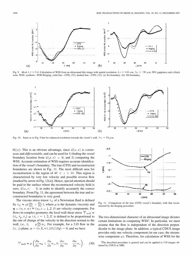
Fig. 9. Mesh 1, t = 0:2. Calculation of WSS from an ultrasound-like image with spatial resolution �x = 140 �m, �z = 130 �m, 50% gappiness and a blackzone. WSS: symbols—POD-Kriging, solid line—CFD, (32), dashed line—CFD, (33). (a) Xa-boundary. (b): Xb-boundary.

Fig. 10. Same as in Fig. 9 but for enhanced resolution towards the vessel’s wall, �x = 93 �m.

. This is an obvious advantage, since is contin-uous and differentiable, and can be used for 1) finding the vesselboundary location from , and 2) computing theWSS. Accurate estimation of WSS requires accurate identifica-tion of the vessel’s boundary. The true (CFD) and reconstructedboundaries are shown in Fig. 11. The most difficult area forreconstruction is the region of . This region ischaracterized by very low velocity and possible reverse flow[marked by arrow in Fig. 12(a)]. Hence, special attention shouldbe paid to the surface where the reconstructed velocity field iszero, , in order to identify accurately the correctboundary. From Fig. 11, the agreement between the true and re-constructed boundaries is very good.

The viscous stress tensor of a Newtonian fluid is definedby , where is the dynamic viscosity and

are velocity components. Forflows in complex geometry, the local wall shear stress

is defined to be proportional tothe rate of change of the velocity in the direction normal to thewall, i.e., . For example, for a 2-D flow in the

-plane, , and we have

(30)

Fig. 11. Comparison of the true (CFD) vessel’s boundary with that recon-structed by the Kriging procedure.

The two-dimensional character of an ultrasound image dictatescertain limitations in computing WSS2. In particular, we mustassume that the flow is independent of the direction perpen-dicular to the image plane. In addition, a typical CDUS imageprovides only one velocity component (in our case, the stream-wise component ). Therefore, for calculation of WSS for the

2The described procedure is general and can be applied to 3-D images ob-tained by CDUS or MRI.


Fig. 12. Reconstruction of the axial w-velocity field, t = 0:2. (a) CFD: anarrow shows a back-flow region with negative velocity. (b) An ultrasound-likeimage, Mesh 1, 50% gappiness with a black zone (hole). (c) Image shown in(b) after POD-K.

synthesized CDUS image considered in this paper, we used thefollowing approximation

(31)

The partial derivatives are calculatedanalytically; on the boundary, their values are computed underthe constraint . For the CFD data, the wall shearstress was computed by two different ways

(32)

and

(33)

Using the expression in (32) is more appropriate for the ultra-sound-like image considered in this study because (33) requiresthe derivative along the direction perpendicular to the image,which is assumed to be unavailable from a typical 2-D CDUSimage. Figs. 9 and 10 show a comparison of the WSS calculatedafter applying the POD-Kriging procedure for the ultrasound-like image. In Fig. 9, we show results obtained on the coarseMesh 1 with m m. The WSS on thelower Xb-boundary is affected by its “wavy” form (see Fig. 11)

Fig. 13. Reconstruction of the axial w-velocity field in the bifurcation region,t = 0:2; (a)—CFD; (b)—an ultrasound-like image, low resolution Mesh 1, 50%gappiness; (c)—the image shown in (b) after POD-K.

which could not be properly captured on the coarse Mesh 1. Theresults in Fig. 10 were obtained on a similar mesh but refinedby a factor of 1.5 along the direction, i.e., m.The improvement of the WSS computed on the Xb-boundarywith slightly finer mesh is significant and it points to the sensi-tivity of WSS calculation. The relative errors are summarized inTable III.

B. Noisy Data

In this section, we present the results of noisy data reconstruc-tion by applying the POD-Kriging procedure enhanced with en-semble or phase averaging and smoothing of the noisy PODmodes. In particular, we use the same CFD results as beforeby taking 101 snapshots of the -velocity field for a selectedpart of the CCA. Fig. 16(a) shows the snapshot at at across-section shown in Fig. 7(a). Speckle (Rayleigh) noise with


Fig. 14. SNR (a) and noise energy (b); open circles indicate the time instances when the WSS was computed.

TABLE IIIRELATIVE ERRORS BETWEEN COMPUTED WSS

AND THE “TRUE” WSS (t = 0:2)

TABLE IVRELATIVE (PERCENTAGE) ERRORS IN RECONSTRUCTING TEMPORAL

(� ) AND SPATIAL (� ) POD MODES OF NOISY DATA

nonzero mean was added at each grid point of the snapshot [seeFig. 16(b)], with SNR ( ). This procedure was repeated30 time yielding 30 realizations (ensemble). A sample of thenoisy flow field is shown in Fig. 16(c). In practice, this ensemblecan be obtained from a single measurement over 30 cardiac cy-cles in which not every one is identical due to either uncertain-ties in measurements or due to pathological effects of a diseasedartery.

1) POD Noisy Modes: The ensemble-mean velocity field,, can now be decomposed further in space-time using

the POD procedure described in Section II-A as follows:

(34)

However, the field is still noisy [see Fig. 16(d)] be-cause the added speckle noise has nonzero ensemble-mean. Wenote that the shape of the first temporal mode, , resemblesthe flow rate and is affected little by the added noise comparedto the higher modes, consistent with the hierarchical nature ofthe POD representation. In contrast to the temporal modes, allspatial modes are noisy as they are obtained from (6) which em-ploys the noisy velocity field, see Fig. 16(d)

The normalized POD eigenspectrum is plotted in Fig. 15 andshows relatively smaller contribution of the third and fourthmodes to the final field. It is also clear that the POD modes withindex do not contribute at all to the reconstruction afterthe ensemble averaging is performed.

Fig. 15. Eigenvalues of the w-velocity POD modes of the CFD data (noise-free), ensemble-averaged and reconstructed by POD-Kriging procedure data.

As the final step of the denoising procedure, the spatialand temporal POD modes are smoothed using the smoothingmethod described in Section II-D. The relative reconstructionerrors of the first four modes are summarized in Table IV.The values in Table IV deserve some comments. Due to thehierarchical nature of the POD modes, the amplitudes of thehigher modes are very small, so that even small amounts ofnoise may totally corrupt the modes rendering them unrecov-erable. Therefore, the POD expansion should be truncatedsince the corrupted tail would only introduce noise to the finalfield. Such truncation corresponds to simple cutoff filtering.In our simulations, the number of modes chosen for the PODreconstruction is since it yields the maximum SNR.

In Fig. 14, we plot SNR and NMR before and after the POD-based smoothing. The initial of the noisy data wasincreased to about 25 after the ensemble averaging. The level ofthe initial noise is about 22% of the velocity mean value. Thefinal SNR ranges between indicating theeffectiveness of the applied procedure. Finally, the color map ofthe reconstructed velocity is shown in Fig. 16.

2) Vessel Wall Location and WSS: We repeated the calcula-tion of the WSS described in Section III-A.3 but for the noisydata for four time instants as indicated in Figs. 2 and 14. Thetime is close to the peak systolic phase whileto the deceleration phase with reverse flow present in the ICAin the vicinity of the stenosis throat. The flow field for these twospecific time instants are particularly difficult for flow recon-


Fig. 16. Reconstruction of the axial w-velocity field from noisy data, t = 0:2;(a)—CFD; (b)—distribution of speckle noise; (c)—noisy data (ultrasound-likeimage); (d)—the image shown in (c) after ensemble averaging (still noisy);(e)—the image shown in (d) after POD-K.

struction so we present results for these instants. The two othertime instants ( and ) are inside the diastolic phase.

As seen in Figs. 9 and 10, increasing the resolution in the di-rection improved the WSS on the Xb-boundary. Hence, in orderto calculate the WSS for the noisy data, we used m.The results are sensitive to the set of parameters specified forsmoothing and Kriging interpolation. The correlation parame-ters of the spline kernel in (21) were chosen to provide the bestagreement with WSS of the CFD simulation. For comparison,we created a test case when 1) the CFD data is noise-free and2) the parameters of Kriging are the same as those used for thenoisy data. We refer to this case as “Kriging (noise-free)”. We

recall that for the noisy data the smoothing parameters were tar-geted to provide the maximum SNR, but here we use a differentcriterion as we focus on WSS.

Fig. 17 shows the WSS calculated after applying the POD-Kriging procedure for noisy ultrasound-like images. The agree-ment with the CFD-based WSS is very good except in the re-gion , where the velocity is very low and reverseflow possible near the upper Xa-boundary [see Fig. 16(a)]. Thedata scattering near the edge indicates that Kriginginterpolation and smoothing alone fail to completely recoverthe correct information there. We note, however, that the agree-ment with the “Kriging (noise-free)” case is excellent but onthe Xb-boundary both results differ from the WSS obtained fora gappy data set shown in Fig. 10(b). This is attributed to the useof different correlation parameters (see Table V) employed forthe gappy and noisy cases due to different optimization criteria.Relative errors are summarized in Table VI. Sensitivity of the re-sults to different correlation parameters is shown in Table VII.

Kriging-based interpolation was used for finding fromthe vessel boundary shown in Fig. 18. For

and , the agreement with the “true” (CFD)boundary is very good except in the low-velocity region. Wenote that similar comparisons performed for andshown excellent agreement.

IV. SUMMARY AND DISCUSSION

Advanced reconstruction of clinical images can significantlyenhance the quality of images in cardiovascular medicine andalso provide missing information in space or time. In thispaper, we considered some prototype cases to reconstruct bothin time and space gappy and noisy data in a carotid artery.The new reconstruction method we proposed is based on theprinciples of evolving dynamic systems and optimum statisticalspace interpolation. In particular, we propose to apply 1) PODfor processing medical images collected over a time interval(snapshots), and 2) Kriging interpolation to black zones andto images with low resolution (i.e., at subpixel level). Wefound that for certain cases of practical interest combining bothapproaches (POD-K) yields the best performance for typicalultrasound-like images.

In particular, we aimed to systematically test and evaluate theeffectiveness of the proposed reconstruction procedure. We havesuccessfully applied the POD-Kriging method so far to limitedclinical data (see example in Figure 1) but we could not eval-uate the effectiveness of our method due to the lack of “true”data sets. To this end, in this paper we synthesized a prototypeof clinical data from high-resolution CFD data sets with the ve-locity field data obtained from 3-D CFD simulations of flowthrough a carotid artery. Our major concern was to have reli-able accurate numerical data sets to compare with. Admittedly,the Reynolds number in our simulations was relatively low forcomputational expedience since in the reconstruction processof the data sets considered in this paper only a few POD modeswere required and this made our parametric study easier to com-plete. However, this does not mean that the method will fail forpatient-specific data as it is general. For example, the presenceof stenosis may trigger transition from laminar to turbulent flowin carotid artery even for flow with moderate Reynolds number.


Fig. 17. Speckle noise, SNR � 5; spatial resolution �x = 93 �m, �z = 130 �m. Calculation of WSS at different time instants t = 0:12 (left) and t = 0:2

(right). The first row shows results for the upper boundary Xa and the second row results for the lower boundary Xb. (a) t = 0:12, (b) t = 0:2, (c) t = 0:12,(d) t = 0:2.

TABLE VCORRELATION PARAMETERS OF KRIGING INTERPOLATION (SPLINE KERNEL)

TABLE VISPECKLE NOISE. RELATIVE ERRORS BETWEEN WSS COMPUTED

ON MESH 2 AND THE “TRUE” WSS

TABLE VIISPECKLE NOISE. COMPARISON OF RELATIVE ERRORS BETWEEN WSS AND

THE “TRUE” WSS FOR DIFFERENT CORRELATION PARAMETERS

(MESH 2, t = 0:2)

In that case, the POD-based reconstruction is also possible butthe number of modes needed for accurate reconstruction will behigher.

Our method treats medical images with spatio-temporalgappy (incomplete) and noisy data and can be applied inconjunction with other methods dealing with correction andpossible elimination of artifacts [29]. In this study, spatio-tem-poral gappiness was first created by discarding some datapoints of the CFD simulation at random. This is supposed tomimic a CDUS image with artifacts, although in real CDUSthe velocity data is intrinsically convolved with a point spreadfunction and there are no values representing the velocity at gridpoints. Another possibility is to assign a specific confidencelevel at each data point, i.e., a weight between zero and one,the latter value corresponding to the case for which we knowthe point value of velocity for sure. This, however, requiresadditional information or assumptions that may complicate thecomparative study we aimed for in the present work. To thisend, our approach can be interpreted as a case with confidencelevels of zero for the points discarded and one for the pointsfor which we know the velocity values for sure. On the otherhand, the creation of regions wherein the data are missing atall times—what we referred to as black zones—representsscenarios where no data are acquired there due to an obstructedview. We note that the POD method fails in the presence ofa black zone but the Kriging procedure we employed is veryeffective in recovering the missing information.


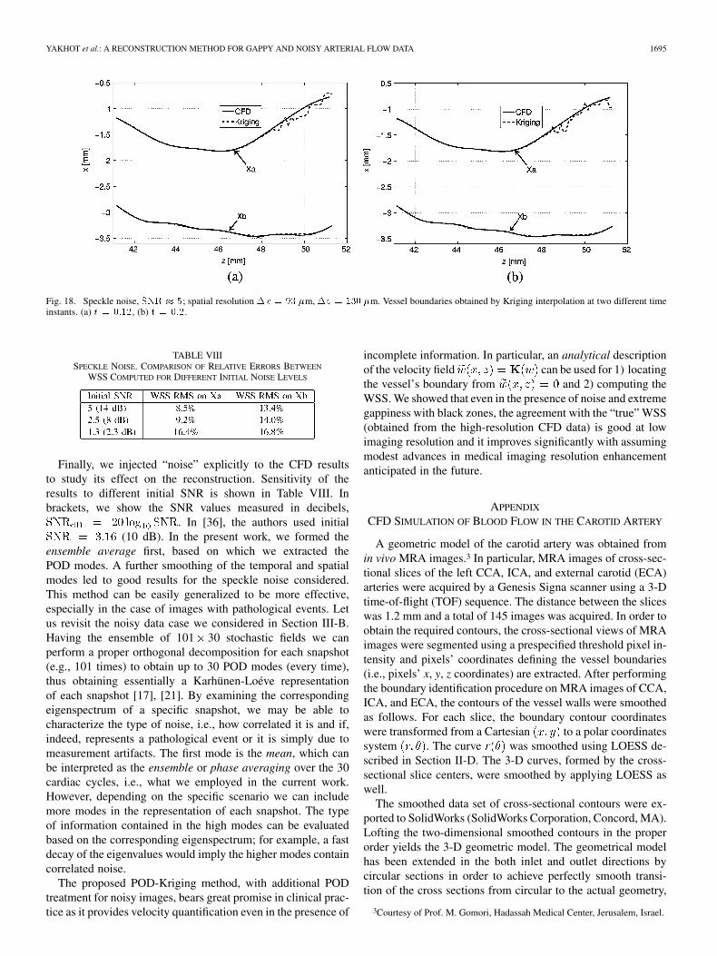
Fig. 18. Speckle noise, SNR � 5; spatial resolution �x = 93 �m, �z = 130 �m. Vessel boundaries obtained by Kriging interpolation at two different timeinstants. (a) t = 0:12, (b) t = 0:2.

TABLE VIIISPECKLE NOISE. COMPARISON OF RELATIVE ERRORS BETWEEN

WSS COMPUTED FOR DIFFERENT INITIAL NOISE LEVELS

Finally, we injected “noise” explicitly to the CFD resultsto study its effect on the reconstruction. Sensitivity of theresults to different initial SNR is shown in Table VIII. Inbrackets, we show the SNR values measured in decibels,

. In [36], the authors used initial(10 dB). In the present work, we formed the

ensemble average first, based on which we extracted thePOD modes. A further smoothing of the temporal and spatialmodes led to good results for the speckle noise considered.This method can be easily generalized to be more effective,especially in the case of images with pathological events. Letus revisit the noisy data case we considered in Section III-B.Having the ensemble of 101 30 stochastic fields we canperform a proper orthogonal decomposition for each snapshot(e.g., 101 times) to obtain up to 30 POD modes (every time),thus obtaining essentially a Karhünen-Loéve representationof each snapshot [17], [21]. By examining the correspondingeigenspectrum of a specific snapshot, we may be able tocharacterize the type of noise, i.e., how correlated it is and if,indeed, represents a pathological event or it is simply due tomeasurement artifacts. The first mode is the mean, which canbe interpreted as the ensemble or phase averaging over the 30cardiac cycles, i.e., what we employed in the current work.However, depending on the specific scenario we can includemore modes in the representation of each snapshot. The typeof information contained in the high modes can be evaluatedbased on the corresponding eigenspectrum; for example, a fastdecay of the eigenvalues would imply the higher modes containcorrelated noise.

The proposed POD-Kriging method, with additional PODtreatment for noisy images, bears great promise in clinical prac-tice as it provides velocity quantification even in the presence of

incomplete information. In particular, an analytical descriptionof the velocity field can be used for 1) locatingthe vessel’s boundary from and 2) computing theWSS. We showed that even in the presence of noise and extremegappiness with black zones, the agreement with the “true” WSS(obtained from the high-resolution CFD data) is good at lowimaging resolution and it improves significantly with assumingmodest advances in medical imaging resolution enhancementanticipated in the future.

APPENDIX

CFD SIMULATION OF BLOOD FLOW IN THE CAROTID ARTERY

A geometric model of the carotid artery was obtained fromin vivo MRA images.3 In particular, MRA images of cross-sec-tional slices of the left CCA, ICA, and external carotid (ECA)arteries were acquired by a Genesis Signa scanner using a 3-Dtime-of-flight (TOF) sequence. The distance between the sliceswas 1.2 mm and a total of 145 images was acquired. In order toobtain the required contours, the cross-sectional views of MRAimages were segmented using a prespecified threshold pixel in-tensity and pixels’ coordinates defining the vessel boundaries(i.e., pixels’ x, y, z coordinates) are extracted. After performingthe boundary identification procedure on MRA images of CCA,ICA, and ECA, the contours of the vessel walls were smoothedas follows. For each slice, the boundary contour coordinateswere transformed from a Cartesian to a polar coordinatessystem . The curve was smoothed using LOESS de-scribed in Section II-D. The 3-D curves, formed by the cross-sectional slice centers, were smoothed by applying LOESS aswell.

The smoothed data set of cross-sectional contours were ex-ported to SolidWorks (SolidWorks Corporation, Concord, MA).Lofting the two-dimensional smoothed contours in the properorder yields the 3-D geometric model. The geometrical modelhas been extended in the both inlet and outlet directions bycircular sections in order to achieve perfectly smooth transi-tion of the cross sections from circular to the actual geometry,

3Courtesy of Prof. M. Gomori, Hadassah Medical Center, Jerusalem, Israel.


Fig. 19. Carotid artery obtained from in vivo MRA images.

TABLE IXGEOMETRIC PARAMETERS OF THE CAROTID ARTERY

TABLE XCOMPUTATIONAL MESH PARAMETERS. CCA; BR; ICA; ECA

see Fig. 19. The modified geometry can readily accommodatefully-developed Womersley flow conditions. The parameters ofthis artery are summarized in Table IX and a 3-D perspectiveis shown in Fig. 19. The original geometry is in red while theextensions are in black.

The geometric model of the artery is then loaded to the meshgenerator GAMBIT to generate the computational mesh, whichis divided into four subdomains: 1) CCA), 2) bifurcation region(BR), 3) internal carotid (ICA), and 4) ECA arteries. A nonuni-form mesh was used with elements clustering near the walls andin the regions with expected complex flow, e.g., bifurcation andstenosis. The CCA, ICA, and ECA subdomains are meshed byhexahedral mesh generation using the multiaxis Cooper’s algo-rithm, while BR was meshed using tetrahedral volume meshesdue to its structural complexity. The number of computationalnodes in subdomains are summarized Table X.

We have employed two different approaches to perform CFDsimulations at several resolutions of 3-D pulsatile flow throughthe carotid artery. The governing equations are the 3-D time-de-pendent Navier-Stokes (NS) equations, subjected to the incom-pressibility constraint. The simulations were performed basedon the finite volume method using the commercial code Fluent(v6.2, Lebanon, New Hampshire). For verification purposes wealso performed selective simulations using the code NEKTARbased on the spectral/ element method [16]. We employed amesh with 36 926 tetrahedral elements of polynomial order 4and second-order time accurate integration. In all tested casesthe difference in the velocity profiles obtained with the twomethods was less than 2%.

The simulations were performed as follows. Starting froman arbitrary initial field a stationary limit cycle was achievedafter ten cardiac cycles. With regards to boundary conditions, aDirichlet condition based on the flow rate shown in Fig. 2

was used at the CCA inlet. This profile was approximated byFourier modes, i.e.,

. Here is the main frequency and arethe coefficients of the Fourier expansion. A fully developed ve-locity profile was prescribed at the proximal end of the CC arteryusing superposition with the well-known Womersley analyticalprofile [34] for each Fourier mode of the flow rate curve. Atthe distal end of the IC and EC arteries, zero pressures wereimposed. No-slip boundary conditions were prescribed at thevessel walls. In our simulations, the kinematic viscosity

mm /s and main frequency s . The Reynoldsnumber , where is the peak systolicmean velocity, and is the CCA inflow cross-section diameter;the Womersley number .

ACKNOWLEDGMENT

The authors are deeply indebted to anonymous reviewers forthe insightful comments that helped them to improve the qualityand content of this paper and wish to express their appreciationto Dr. D. Venturi for valuable discussions.

REFERENCES

[1] J. G. Abboti and F. L. Thurstone, “Acoustic speckle: Theory and ex-perimental analysis,” Ultrason. Imag., vol. 1, pp. 303–324, 1979.

[2] G. Bambi, T. Morganti, S. Rici, E. Boni, F. Guidi, C. Palombo, andP. Tortoli, “A novel ultrasound instrument for investigation of arterialmechanics,” Ultrasonics, vol. 42, pp. 731–737, 2004.

[3] D. C. Barratt, B. Ariff, K. N. Humphries, S. A. Thom, and A. D.Hughes, “Reconstruction and quantification of the carotid arterybifurcation from 3-D ultrasound images,” IEEE Trans. Med. Imag.,vol. 35, no. 5, pp. 567–583, May 2004.

[4] V. Behar, D. Adam, and Z. Friedman, “A new method of ultrasoundcolor flow mapping,” Ultrasonics, vol. 41, pp. 385–395, 2003.

[5] L. Bohs, S. Gebhart, and M. Anderson, “2-D motion estimation usingtwo parallel receive beams,” IEEE Trans. Ultras. Ferroelectr. Freq.Contr., vol. 48, no. 2, pp. 392–408, Mar. 2001.

[6] P. J. Brands, A. P. G. Hoeks, L. Hofstra, and R. S. Reneman, “A nonin-vasive method to estimate wall shear rate using ultrasound,” Ultr. Med.Biol., vol. 21, pp. 171–185, 1995.

[7] M. Calzolai, L. Capineri, A. Fort, L. Masotti, S. Rocchi, and M. Scabia,“A 3-D PW Ultrasonic doppler flow-meter: Theory and experimentalcharacterization,” IEEE Trans. Ultrason. Ferroelectr. Freq. Contr., vol.46, pp. 108–113, 1999.

[8] C. G. Caro, J. M. Fitz-Gerald, and R. C. Schroter, “Atheroma and arte-rial wall shear: Observation, correlation and proposal of shear depen-dent mass transfer for atherogenesis,” Proc. R. Soc. Lond. B, vol. 177,pp. 109–159, 1971.

[9] W. S. Cleveland and S. J. Devlin, “Locally weighted regression: Anapproach to regression analysis by local fitting,” J. Am. Statist. Assoc.,vol. 83, pp. 596–610, 1988.

[10] R. M. Everson and L. Sirovich, “The Karhunen-Loève transform forincomplete data,” J. Opt. Soc. Am. A, vol. 12, no. 8, pp. 1657–1664,1995.

[11] M. D. Fox and W. Cardiner, “Three-dimensional Doppler velocimetryof flow jets,” IEEE Trans. Biomed. Eng., vol. 35, no. 10, pp. 834–841,Oct. 1988.

[12] D. P. Giddens, C. K. Zarins, and S. Glagov, “The role of fluidmechanics in the localization and detection of artherosclerosis,” J.Biomech. Eng., vol. 115, pp. 588–594, 1993.

[13] H. Gunes, S. Sirisup, and G. E. Karniadakis, “Gappy data: To Krig ornot to Krig?,” J. Comp. Phys., vol. 212, pp. 358–382, 2006.

[14] A. P. G. Hoeks, S. K. Samijo, P. J. Brands, and R. S. Reneman, “Non-invasive determination of shear-rate distribution across the arteriallumen,” Hypertension, vol. 26, pp. 26–33, 1995.

[15] P. Holmes, J. L. Lumley, and G. Berkooz, Turbulence, Coherent Struc-tures, Dynamical Systems and Symmetry. Cambridge, U.K.: Cam-bridge Univ. Press, 1996.

[16] G. E. Karniadakis and S. J. Sherwin, Spectral/hp Element Methods forComputational Fluid Dynamics. Oxford, U.K.: Oxford Univ. Press,2005.


[17] M. Kirby, Geometric Data Analysis: An Empirical Approach to Dimen-sionality Reduction and the Study of Patterns. New York: Wiley-In-terscience, 2000.

[18] U. Köhler, I. Marshall, M. B. Robertson, Q. Long, X. Xu, and P. R.Hoskins, “MRI measurements of the wall shear stress vectors in bifur-cation models and comparison with CFD predictions,” J. Magn. Reson.Imag., vol. 14, pp. 563–573, 2001.

[19] D. N. Ku, D. P. Giddens, C. K. Zarins, and S. Glagov, “Pulsatile flowand atherosclerosis in the human carotid bifurcation. Positive correla-tion between plaque location and low oscillating shear stress,” Arte-riosclerosis, vol. 5, pp. 293–302, 1985.

[20] S. Lophaven, H. Nielsen, and J. Sondergaard, Informatics and mathe-matical modeling DTU, Rep. IMM-REP-2002-12, 2002.

[21] M. Loéve, Probability Theory, 4th ed. New York: Springer-Verlag,1977.

[22] A. Loupas, “Digital Image Processing for Noise Reduction in MedicalUltrasonics,” Ph.D., Univ. Edinburgh, Edinburgh, U.K., 1988.

[23] I. Marshall, S. Zhao, P. Papathanasopoulou, P. Hoskins, and X. Y. Xu,“MRI and CFD studies of pulsatile flow in healthy and stenosed carotidbifurcation models,” J. Biomech., vol. 37, pp. 679–687, 2004.

[24] J. A. Moore, D. A. Steinman, and C. R. Ethier, “Computational bloodflow modelling: Errors associated with reconstructing finite elementmodels from magnetic resonance images,” J. Biomech., vol. 31, pp.179–184, 1998.

[25] S. Oyre, S. Ringgaard, S. Kozerke, W. P. Paaske, M. Erlandsen, P. Boe-siger, and E. M. Pedersen, “Accurate noninvasive quantitation of bloodflow, cross-sectional lumen vessel area and wall shear stress by three-dimensional paraboloid modeling of magnetic resonance imaging ve-locity data,” J. Amer. Col. Card., vol. 32, pp. 128–134, 1998.

[26] P. Papathanasopoulou, S. Zhao, U. Köhler, M. B. Robertson, Q. Long,P. Hoskins, X. Y. Xu, and I. Marshall, “MRI measurement of time-resolved wall shear stress vectors in a carotid bifurcation model, andcomparison with CFD predictions,” J. Magn. Res. Imag., vol. 17, pp.153–162, 2003.

[27] M. Sonka and J. Fitzpatrik, Handbook of Medical Imaging, MedicalImage Processing and Analysis. Bellingham, WA: SPIE, 2000, vol.2.

[28] M. Stein, Interpolation of spatial data: Theory for Kriging. Berlin,Germany: Springer, 1999.

[29] D. A. Steinman, C. R. Ethier, and B. K. Rutt, “Combined analysis ofspatial and velocity displacement artifacts in phase contrast measure-ments of complex flows,” J. Magn. Res. Imag., vol. 7, pp. 339–346,1997.

[30] D. A. Steinman, J. B. Thomas, H. M. Ladak, J. S. Milner, B. K. Rutt,and J. D. Spence, “Reconstruction of carotid bifurcation hemody-namics and wall thickness using computational fluid dynamics andMRI,” Magn. Res. Med., vol. 47, pp. 149–59, 2002.

[31] R. Stokholm, S. Oyre, S. Ringgaard, H. Flaagoy, W. P. Paaske, and E.M. Pedersen, “Determination of wall shear rate in the human carotidartery by magnetic resonance techniques,” Eur. J. Vasc. Endovasc.Surg., vol. 20, pp. 427–433, 2000.

[32] J. Suzuki, R. Shimamoto, J. Nishikawa, T. Tomaru, T. Nakajima, F.Nakamura, W. S. Shin, and T. Toyo-oka, “Vector analysis of the hemo-dynamics of atherogenesis in the human thoracic aorta using MR ve-locity mapping,” Amer. J. Roentgenol., vol. 171, pp. 1285–1290, 1998.

[33] D. Venturi and G. E. Karniadakis, “Gappy data and reconstructionprocedures for flow past a cylinder,” J. Fluid Mechan., vol. 519, pp.315–336, 2004.

[34] F. M. White, Viscous Fluid Flow. New York: McGraw-Hill, 1991.[35] S. P. Wu, S. Ringgaard, and E. M. Pedersen, “Three-dimensional phase

contrast velocity mapping acquisition improves wall shear stress esti-mation in vivo,” Magn. Res. Imag., vol. 22, pp. 345–351, 2004.

[36] Y. Zhang, L. Wang, Y. Gao, J. Chen, and X. Shi, “Noise reductionin Doppler ultrasound signals using an adaptive decomposition algo-rithm,” Med. Eng. Phys., vol. 29, pp. 699–707, 2007.

IEEE TRANSACTIONS ON MEDICAL IMAGING, VOL. 26, NO. 12 ...

Documents

Transcript of IEEE TRANSACTIONS ON MEDICAL IMAGING, VOL. 26, NO. 12 ...