IEEE TRANSACTIONS ON AUDIO, SPEECH, AND …bchamp/Papers/Jounal/IEEE-ASLP2008.pdfthis manuscript and...

IEEE TRANSACTIONS ON AUDIO, SPEECH, AND LANGUAGE PROCESSING, VOL. 16, NO. 1, JANUARY 2008 137

A Noise-Robust FFT-Based Auditory SpectrumWith Application in Audio Classification

Wei Chu and Benoît Champagne

Abstract—In this paper, we investigate the noise robustness ofWang and Shamma’s early auditory (EA) model for the calculationof an auditory spectrum in audio classification applications. First,a stochastic analysis is conducted wherein an approximate expres-sion of the auditory spectrum is derived to justify the noise-sup-pression property of the EA model. Second, we present an efficientfast Fourier transform (FFT)-based implementation for the calcu-lation of a noise-robust auditory spectrum, which allows flexibilityin the extraction of audio features. To evaluate the performanceof the proposed FFT-based auditory spectrum, a set of speech/music/noise classification tasks is carried out wherein a supportvector machine (SVM) algorithm and a decision tree learning al-gorithm (C4.5) are used as the classifiers. Features used for clas-sification include conventional Mel-frequency cepstral coefficients(MFCCs), MFCC-like features obtained from the original audi-tory spectrum (i.e., based on the EA model) and the proposed FFT-based auditory spectrum, as well as spectral features (spectral cen-troid, bandwidth, etc.) computed from the latter. Compared to theconventional MFCC features, both the MFCC-like and spectralfeatures derived from the proposed FFT-based auditory spectrumshow more robust performance in noisy test cases. Test results alsoindicate that, using the new MFCC-like features, the performanceof the proposed FFT-based auditory spectrum is slightly betterthan that of the original auditory spectrum, while its computa-tional complexity is reduced by an order of magnitude.

Index Terms—Audio classification, C4.5, early auditory (EA)model, noise suppression, self-normalization, support vectormachine (SVM).

I. INTRODUCTION

RECENT years have seen extensive research on audioclassification algorithms which provide useful informa-

tion for both audio and video content understanding. Amongmany different audio classes in the field of audio classification,the generic classes of speech and music have attracted muchattention. Saunders [1] has used a measure of energy contourand the distribution of zero-crossing rate (ZCR) in discrim-inating speech from music on broadcast FM radio. Scheirerand Slaney [2] proposed to use as many as 13 features, suchas 4-Hz modulation energy, spectral centroid, etc., to classifyspeech and music, where a correct classification rate of 94.2%has been reported for 20-ms segments and 98.6% for 2.4-s

Manuscript received February 16, 2007; revised July 25, 2007. This workwas supported by a grant from the Natural Sciences and Engineering ResearchCouncil of Canada (NSERC). The associate editor coordinating the review ofthis manuscript and approving it for publication was Dr. Hiroshi Sawada.

The authors are with the Department of Electrical and Computer Engineering,McGill University, Montréal, QC H3A 2A7, Canada (e-mail: [email protected]; [email protected]).

Color versions of one or more of the figures in this paper are available onlineat http://ieeexplore.ieee.org.

Digital Object Identifier 10.1109/TASL.2007.907569

segments. Low bit-rate audio coding is another application thatcan benefit from distinguishing speech from music [3], [4].

Besides speech and music, many other audio classes, in-cluding environmental sounds and background noise, have beeninvestigated. In [5], a system for content-based classification,search, and retrieval of audio signals is presented wherein awide variety of sounds are selected from animals, machines,musical instruments, speech, and the nature. Zhang and Kuo[6] have proposed a hierarchical system for audio classificationand retrieval where audio clips are first classified and seg-mented into speech, music, environmental sounds, and silence;the environmental sounds are then further classified into tenclasses using a hidden Markov model (HMM). Lu et al. [7]also proposed a two-stage robust approach that is capable ofclassifying and segmenting an audio stream into speech, music,environment sound, and silence. In [8] and [9], special soundeffects which are related to entertainment or sport events, suchas laughter, scream, etc., have been investigated. Mixed orhybrid sounds have also been studied, for example, speech withnoise or music background, environmental sound with musicbackground, etc. [10], [11]. Recently, a fuzzy approach wasproposed where a fuzzy class is reserved for input audio thatcannot be classified as pure speech, music, or silence [12].

Despite the growing interest in audio classification al-gorithms, as seen from the above references, the effect ofbackground noise on the classification performance has notbeen investigated widely. In fact, a classification algorithmtrained using clean sequences may fail to work properly whenthe actual testing sequences contain background noise withcertain signal-to-noise ratio (SNR) levels (see test results in[13]–[16]). For example, results from [13] show that, using a setof Mel-frequency cepstral coefficients (MFCCs) as features, theerror rate of speech/music classification increases significantlyfrom 0% in a clean test to 41% in a test where SNR 10 dB.For practical applications wherein environmental sounds areinvolved in audio classification tasks, noise robustness is anessential characteristic of the processing system.

Recently, the early auditory (EA) model presented by Wangand Shamma [17] has been employed in a two-class audio classi-fication task (i.e., speech/music using a Gaussian mixture modelas the classifier), and robust performance in noisy environmentshas been reported [13]. For example, at SNR 15 dB, the errorrate of the auditory based features is 17.7% compared to 40.3%for the conventional MFCC features. The EA model calculatesa so-called auditory spectrum based on a series of linear andnonlinear processing steps including filtering with a set of con-stant- bandpass filters. According to the analysis in [17], thenoise-robustness of the EA model can be attributed in part to itsself-normalization property which causes spectral enhancement

1558-7916/$25.00 © 2007 IEEE

Authorized licensed use limited to: McGill University. Downloaded on June 3, 2009 at 11:41 from IEEE Xplore. Restrictions apply.

138 IEEE TRANSACTIONS ON AUDIO, SPEECH, AND LANGUAGE PROCESSING, VOL. 16, NO. 1, JANUARY 2008

or noise suppression. These conclusions on the self-normaliza-tion property are obtained using a qualitative analysis first, fol-lowed by a quantitative analysis wherein a closed-form expres-sion of the auditory spectrum is derived. Due to the nonlinearityof the EA model, for the quantitative analysis, only a specialsimplified case has been studied wherein a step function is usedto replace the original nonlinear sigmoid compression function.With respect to the limitation of the quantitative analysis in [17],it is of interest to investigate the noise-suppression propertyfrom a broader perspective, i.e., to derive a closed-form expres-sion for auditory spectrum using a more general sigmoid-likefunction, and to conduct relevant analysis.

The noise-robustness of the original EA model has beendemonstrated in different applications [13], [16], [17]. How-ever, this model is characterized by high computationalrequirements and the use of nonlinear processing. It is thereforedesirable to derive an approximated version of the EA modelin the frequency domain, where efficient fast Fourier trans-form (FFT) algorithms are available. In an earlier study [16],we proposed such a simplified FFT-based spectrum whereina local self-normalization scheme is implemented. Resultsfrom a speech/music/noise classification task show that theperformance of the proposed FFT-based spectrum is compa-rable to that of the original EA model while its computationalcomplexity is much lower. This FFT-based spectrum employsa simple grouping scheme to reduce the dimension of thepower spectrum vector. However, this scheme fails to give aclear interpretation of the meaning of the frequency index. Inapplications where frequency-dependent audio features needto be extracted (e.g., spectral centroid, bandwidth), it wouldbe more appropriate, instead of this simple grouping scheme,to group or select power spectrum components based on theoriginal constant- bandpass filters.

In this paper, first, we extend the analysis in [17] by investi-gating the noise-suppression property of the EA model from amore general perspective wherein a closed-form expression ofthe auditory spectrum is derived by using Gaussian cumulativedistribution function (CDF) as an approximation to the originalsigmoid compression function. Second, an improved implemen-tation is presented for the calculation of an FFT-based auditoryspectrum which extends our previous work in [16]. The intro-duced improvements include the use of characteristic frequency(CF) values of the cochlear filters in the EA model for powerspectrum selection, and the use of a pair of fast and slow run-ning averages over the frequency axis for the implementation ofthe self-normalization. With these improvements, the proposedFFT-based auditory spectrum allows flexibility in the extractionof noise-robust audio features.

To evaluate the noise-robustness of the proposed FFT-basedauditory spectrum, a three-class (i.e., speech/music/noise) audioclassification task is carried out wherein a support vector ma-chine (SVM) algorithm and a decision tree learning algorithm(C4.5 [18]) are employed for classification. Audio featuresused in this work include: conventional Mel-frequency cepstralcoefficients (MFCCs), MFCC-like features obtained from theoriginal auditory spectrum (i.e., based on the EA model), andthe proposed FFT-based auditory spectrum, as well as spectralfeatures (spectral centroid, bandwidth, etc.) computed from

the latter. Compared to the conventional MFCC features, theMFCC-like features and the spectral features derived fromthe original or the proposed FFT-based auditory spectra showmore robust performance in noisy test cases. It is also notedthat, using the new MFCC-like features, the performance of theproposed FFT-based auditory spectrum is slightly better thanthat of the original auditory spectrum, while its computationalcomplexity is reduced by an order of magnitude, i.e., a factor of10 or more. The robustness of the MFCC-like features derivedfrom the proposed FFT-based auditory spectrum is furtherconfirmed by test results of noise/non-noise classificationexperiments.

The paper is organized as follows. The EA model presentedby Wang and Shamma [17], together with the original analysisof its noise-robustness property, are summarized in Section II.As an extension to this original analysis, the proposed analysisof self-normalization based on Gaussian cumulative distributionfunction is presented in Section III. The improved implemen-tation for the calculation of the FFT-based auditory spectrumis detailed in Section IV. Section V discusses the extraction ofaudio features and the setup of the classification tests. Test re-sults are presented in Section VI, while Section VII concludesthis work.

II. EA MODEL

A. Structure of the EA Model

In [17] and [19], a computational auditory model is describedbased on neurophysiological, biophysical, and psychoacous-tical investigations at various stages of the auditory system. Itconsists of two basic stages, i.e., an early stage and a centralstage. The former, called the EA model, describes the transfor-mation of the audio signal into an internal neural representationreferred to as auditory spectrogram, whereas the latter analyzesthe spectrogram to estimate the content of its spectral andtemporal modulations. In this paper, we focus on an EA modelwhich can be simplified as a three-stage process as shown inFig. 1 [17]. An audio signal entering the ear first produces acomplex spatio–temporal pattern of vibrations along the basilarmembrane (BM). A simple way to describe the characteristicresponse of the BM is to model it as a bank of constant- highlyasymmetric bandpass filters with impulse responses ,where is the time index and denotes a specific location onthe BM (or equivalently, a channel index).

At the next stage, the motion on the BM is transformed intoneural spikes in the auditory nerves. The process at this stage canbe modeled by the following three steps: a temporal derivativewhich converts instantaneous membrane displacement into ve-locity, a sigmoid compression function which models thenonlinear channel through the hair cells, and a low-pass filter

accounting for the leakage of the cell membranes.At the last stage, a lateral inhibitory network (LIN) detects

discontinuities along the cochlear axis . The operations can bedivided into the following four steps: a derivative with respectto the tonotopic axis which describes the lateral interactionamong LIN neurons, a local smoothing which accountsfor the finite spatial extent of the lateral interactions, a half-wave rectifier (HWR) which models the nonlinearity of the LIN


CHU AND CHAMPAGNE: NOISE-ROBUST FFT-BASED AUDITORY SPECTRUM 139

Fig. 1. Schematic description of the early auditory model [17].

neurons, and a temporal integration which reflects the fact thatthe central auditory neurons are unable to follow rapid temporalmodulations.

These operations effectively compute a spectrogram of anacoustic signal. At a specific time index , the outputis referred to as an auditory spectrum.

B. Noise Robustness of the EA Model

In [17], through a stochastic analysis, this EA model is provedto be noise robust due to an inherent self-normalization prop-erty. The main results of this analysis are summarized next.

1) Qualitative Analysis of the Self-Normalization Property:Suppose the input signal can be modeled as a randomprocess with zero mean. If the bandwidth of the temporal inte-grator in Fig. 1 is narrow enough, the output auditory spectrum

can be approximated by [17], wheredenotes statistical expectation; is referred to as anauditory spectrum in [17].

For the sake of simplicity, the temporal and spatial smoothingfilters and are ignored in the analysis [17]. Definequantities and as1

(1)

(2)

where denotes the time-domain convolution. It can be shownthat

(3)

where denotes the probability density function (pdf) ofat given and the derivative function is assumed

nonnegative. Based on (3), the following qualitative conclusionsare reached in [17].

1) The auditory spectrum is proportional to the en-ergy of [due to the quantity in (3)], andinversely proportional to the energy of (due to function

), where and are defined in (1) and (2).2) Considering that the cochlear filters are broad while

the differential filters are narrow and cen-tered around the same frequencies, can be viewed as asmoothed version of .

1The dependence of U and V on indices (t; s) is dropped in the main text fornotational simplicity.

3) Combining 1 and 2, the auditory spectrum is a self-normal-ized spectral profile. Specifically, a spectral peak receivesa relatively small self-normalization factor (i.e., the energyof is relatively small), whereas a spectral valley receivesa relatively large self-normalization factor.

4) The above difference in the self-normalization further en-larges the ratio of spectral peak to valley, a phenomenonreferred to as spectral enhancement or noise suppression.

2) Quantitative Analysis of a Special Case: It is desirablethat the above qualitative analysis on the self-normalizationproperty be verified by some results of a quantitative nature.However, due to the nonlinearity of the EA model, it is difficultto find a simple closed-form expression for the integral in (3).

In [17], a special case has been studied wherein the hair cellnonlinear sigmoid compression function is replaced by astep function; in this case, becomes a delta function .Assuming the input signal is a zero mean Gaussian process,(3) can be expressed in closed form as

(4)

where , and denote the correlation coefficient betweenand , the standard deviation of , and the standard deviationof , respectively. This expression demonstrates the self-nor-malization nature of the auditory spectrum as analyzed above,i.e., is proportional to the standard deviation2 ofand inversely proportional to that of .

III. ANALYSIS OF THE SELF-NORMALIZATION PROPERTY

Although a step function can be treated as a very special caseof the sigmoid compression function in Fig. 1, it is desir-able to obtain the closed-form expression of usinga better, yet mathematically tractable, approximation. In par-ticular, it is of interest to determine whether the resulting ex-pression still supports the original analysis on self-normaliza-tion based on a step function. Having noticed the general non-linear compression nature of the Gaussian cumulative distribu-tion function (CDF), and the resemblance between the graph ofthe sigmoid function and that of the Gaussian CDF, below, weuse Gaussian CDF as an approximation to the sigmoid compres-sion function to derive a closed-form expression ofand conduct relevant analysis.

2In [17], considering the one-to-one correspondence between the standarddeviation � and the variance � , the former is referred to as energy.



Fig. 2. Sigmoid function (� = 0:1) and Gaussian distribution function (� = 0:163). (a) g(x) and �(x=� ). (b) g (x) and (1=� )� (x=� ).

A. Approximation to the Sigmoid Compression Function

Referring to Fig. 1, the sigmoid compression function at thehair cells stage takes the form of [20]

(5)

where the coefficient is set to 0.1.Fig. 2(a) shows the sigmoid function with . By

inspecting (5) and Fig. 2(a), it is noted that resembles theCDF of a Gaussian random variable with zero mean. In partic-ular, with in (5), is close to the CDF of a Gaussianvariable with zero mean and standard deviation , i.e.,

, where is the CDF of a standard normal randomvariable as defined as follows:

(6)

The function is also shown in Fig. 2(a). The deriva-tives of the function and , respectively, and

, are shown in Fig. 2(b). The relative differencebetween the two curves in Fig. 2(b) over a practical range ofvalues of , as determined from experimental measurements,is of the order of 2% or less for the different processing chan-nels.3

In the following analysis, based on the above considerations,with is approximated as

(7)

where .

3There are 129 channels, corresponding to a set of 129 bandpass filters. SeeSection IV.

Fig. 3. E[y (t; s)] as a function of � and � .

B. Closed-Form Expression of

As in [17], assume the input signal is a zero mean sta-tionary Gaussian process. For given values of , and

are obtained by linear filtering of and are thus zeromean Gaussian random variables, i.e., , and

, where and denotethe standard deviations of and , respectively. According to[21] and [22], the conditional pdf of given , denoted

, is also Gaussian with mean andvariance , where represents the correlationcoefficient between and .

With the assumptions made above, the result of (3) is (seeAppendix I for details)

(8)

From (8), it is noted that is a linear function of. Furthermore, given that , and are all positive

values, and , it is found thatand , which means that is anincreasing function of and a decreasing function of .



Fig. 4. Schematic description of the proposed FFT-based implementation.

Fig. 3 gives a three-dimensional view of as a func-tion of and , where and is set to a fixedvalue of 0.1 to facilitate the analysis.4

The results given in (8) and Fig. 3 indicate that,is proportional to (or, the “energy” of according to [17])and inversely proportional to (or, the “energy” of ac-cording to [17]). Therefore, using a Gaussian CDF to approx-imate the original sigmoid function, the derived results supportthe original analysis on self-normalization which is summarizedin Section II-B1.

C. Local Spectral Enhancement

With respect to the conclusions on self-normalization sum-marized in Section II-B1, statement 4 refers to a desirable sit-uation where spectral enhancement is achieved. It seems to bea natural result from statement 3, but it may not be necessarilythe case.

To facilitate the following analysis on local spectral en-hancement due to the self-normalization property, we assumethat where and are treatedas positive quantities. Suppose that corresponds toa power spectral peak, and is a smoothed version of

. Similarly, and are assumed to be apower spectral valley and its smoothed version, respectively.

In statement 3, the word “relatively” indicates a comparisonbetween the power spectrum component and the correspondingsmoothed version, i.e., we have the following:

(9)

(10)

However, to have the ratio of spectral peak to valley enlarged,the following should be satisfied:

(11)

i.e., it is required that , which may not benecessarily so. In the case with the above simplified assump-tions, (9) and (10) do not necessarily ensure that we have (11).

4According to our tests based on the implementation [20], the mean values ofr for the three audio classes (i.e., speech, music, and noise) in different noiseenvironments are around 0.1.

Thus, the statement 4 is not guaranteed, although it refers to aproperty that is desirable for noise suppression.

Although the enlargement of the ratio of spectral peak tovalley is not guaranteed from the above analysis, conditionsgiven in (9) and (10) do provide a basis for spectral enhance-ment. Given (9) and (10), a simple way to enlarge the ratio ofspectral peak to valley is to multiply the spectral components

and with the corresponding ratios given in (9)and (10), i.e.,

(12)

Next, we will propose a simple FFT-based system wherein theidea presented in (12) is implemented.

IV. NEW AUDITORY-INSPIRED FFT-BASED SPECTRUM

The EA model [17] is characterized by a complicated compu-tation procedure and the use of nonlinear processing. It wouldbe desirable that the model be simplified, or approximated in thefrequency domain where efficient FFT algorithms are available.In our earlier study [16], such a simplified implementation hasbeen proposed to calculate a self-normalized FFT-based spec-trum which is proved to be noise-robust in audio classificationtests.

The FFT-based implementation we proposed in [16] employsa simple grouping scheme to reduce the dimension of the powerspectrum vector. However, this scheme fails to give a clear in-terpretation of the meaning of the frequency index. In applica-tions where frequency-dependent audio features need to be ex-tracted (e.g., spectral centroid, bandwidth), it would be more ap-propriate, instead of the simple grouping scheme we have pro-posed, to group or select power spectrum components based onthe original constant- bandpass filters (see Section II).

In this paper, by making use of the characteristic frequency(CF) values of the bandpass filter set of the EA model [17], andby integrating the self-normalization property through a pair ofrunning averages, we present a new implementation for the cal-culation of the FFT-based spectrum proposed in [16], as illus-trated in Fig. 4. The details of the proposed implementation arepresented next.



TABLE IFREQUENCY INDEX VALUES OF N AND �

Fig. 5. Cochlear filter H(!; s) centered at 1017 Hz and the corresponding dif-ferential filter @ H(!; s). (The 3-dB bandwidth of the cochlear filter is about220 Hz, while the 3-dB bandwidth of the differential filter is 80 Hz.)

A. Normalization of the Input Signal

To make the algorithm adaptable to input signals with dif-ferent energy levels, each input audio clip (with a length of 1 s)is normalized with respect to the square-root value of its averageenergy.

B. Calculation of a Short-Time Power Spectrum

Using the normalized audio signal, a short-time power spec-trum is calculated through an -point FFT algorithm. To deter-mine an appropriate value for , we have to trade performanceagainst complexity.

The cochlear filters in the EA model are modeled as a set ofconstant- bandpass filters [17], [23]. In implementation [20],

Fig. 6. Running average scheme.

the 129 CF values of the corresponding constant- bandpassfilters are determined by5

(13)

where Hz, and .According to (13), the CF values cover a range from 180 to

7246 Hz. The difference between two neighboring CF values isas low as about 5.27 Hz for and . For a signal sampledat 16 kHz, which is used in this study, even with a 2048-pointFFT, such a small frequency interval cannot be resolved. Mean-while, since the CF values are logarithmically located, the fre-quency resolution achieved from a 2048-point or even higherorder FFT algorithm is more than necessary for the high-fre-quency bands. In this paper, we use an -point FFT toachieve a tradeoff between frequency resolution and computa-tional complexity. The length of the analysis window is 30 msand the overlap is 20 ms.

C. Power Spectrum Selection

To reduce the dimension of the obtained power spectrumvector, a simple selection scheme is proposed as follows. First,we extend the values of in (13), i.e., from 10 to 132. Orequivalently, (13) is modified as6

(14)

where . For each , the corresponding fre-quency index is determined by

(15)

where function returns the nearest integer value of , andis the sampling frequency. After discarding the repeated

values and renumbering the remaining values, we obtain a set of

5Instead of 129, the actual size of the output auditory spectrum vector is 128due to the derivative with respect to the channel (see Fig. 1).

6One purpose of extending the values of k is to include more low-frequencycomponents for power spectrum selection. The second purpose is to make thesize of the proposed FFT-based auditory spectrum vector [i.e., 120, see (16)]comparable to that of the original auditory spectrum vector (i.e., 128).



Fig. 7. Proposed FFT-based spectrograms of a 1-s speech clip. (a) Clean case. (b) SNR = 15 dB.

120 characteristic frequency index values , ,as illustrated in Table I.

Using frequency index values , the power spectrum selec-tion (see Fig. 4) is as follows:

(16)

Based on (16), a set of , i.e., 512, power spectrum compo-nents is transformed into a 120-dimensional vector, with eachfrequency index value corresponding to a specific CF value ofthe original cochlear filters.

D. Spectral Self-Normalization

As discussed in Section III-C, the ratio of spectral peak tovalley can be enlarged through the scheme given by (12). In [16],such a local self-normalization is implemented through the useof a pair of wide and narrow windows defined in the frequencydomain. Below, we propose an improved implementation forself-normalization which is simpler and easier to use than theone in [16].

According to [17], the cochlear filters are broad and highlyasymmetric, and the differential filters are narrowly tunedand centered around the same frequencies. Fig. 5 shows themagnitude responses of a cochlear filter , which iscentered at 1017 Hz, and the corresponding differential filter

[20]. Based on the magnitude responses shownin Fig. 5, an iterative running average is defined over thefrequency index as follows:

(17)

where , and and are the input and av-eraged output, respectively. A relatively large corresponds toa “fast” running average, while a relatively small results in a“slow” running average. A slow and fast running averages areemployed here to simulate a cochlear filter and a differentialfilter, respectively.

An example of the running average defined in (17) is illus-trated in Fig. 6, which shows a power spectrum vector in relativevalues and its running averaged version with . In gen-eral, for a spectral peak, the corresponding smoothed value is

smaller, while for a spectral valley, the corresponding smoothedvalue is larger.

Let and represent the outputs from a fast and aslow running averages, respectively. may be viewed as asmoothed version of . Based on and , a self-normalization coefficient at frequency index , , is definedas

(18)

Therefore, in general is larger than 1 for a spectral peakand smaller than 1 for a spectral valley, which coincides withthe conditions given in (9) and (10).

To implement the self-normalization, the selected powerspectrum at frequency index , i.e., , is multiplied by thecorresponding self-normalization coefficient , generatinga set of self-normalized power spectrum data . By usingdifferent parameters for the two running averages, the effectof self-normalization varies, leading to variable classificationperformance (see Section VI-C).

E. Postprocessing

The square-root values of the self-normalized spectrum dataare further calculated. Finally, the proposed auditory-in-

spired FFT-based spectrum is obtained by applying a smoothingoperation on the square-root spectrum data. The smoothing canbe implemented using a fast running average as defined in (17).For the sake of simplicity, the smoothing process is not con-sidered in this paper. Fig. 7 gives an example of the proposedFFT-based spectrograms of a 1-s speech clip in a clean case andin a noisy case where SNR 15 dB. From Fig. 7, we can seethat the two spectrograms are fairly close to each other.

Compared to the self-normalization scheme we proposed in[16], the new implementation presented here is simpler andeasier to use since it only involves two parameters to adjust,i.e., a fast and a slow running average coefficients. Besides, bymaking use of the CF values of the original bandpass filters,a relationship is created between the frequency index of theproposed FFT-based auditory spectrum vector and the physicalfrequency value. Therefore, the proposed FFT-based auditory



spectrum allows more flexibility in the extraction of differentaudio features.

V. FEATURES EXTRACTION AND CLASSIFICATION TESTS

A. Audio Features

In this paper, six sets of frame-level audio features arecalculated, specifically: conventional MFCC features with andwithout cepstral mean subtraction (CMS); MFCC-like featurescomputed from the original auditory spectrum (i.e., the outputof the EA model), from the FFT-based spectrum of [16], andfrom the proposed FFT-based auditory spectrum; as well asspectral features obtained from the FFT-based auditory spec-trum. The corresponding clip-level features are the statisticalmean and variance values of these frame-level features calcu-lated over a 1-s time window. The clip-level features are usedfor the training and testing of the classification algorithm. Thedetails of the frame-level features are given below.

1) Conventional MFCC Features: Being widely used inspeech/speaker recognition, MFCCs [24] are also useful inaudio classification. For the purpose of performance compar-ison, the conventional MFCCs are used in this paper. A Matlabtoolbox developed by Slaney [25] is used to calculate a set of13 conventional MFCCs.

As for the conventional MFCC features, a so-called CMStechnique may improve the robustness of frame-level MFCCsby removing the time averages from the cepstrum data [26]. Inthis paper, we have used a 10-s window to calculate the time av-erages of the MFCCs data needed in the application of the CMSoperation for frame-based MFCCs data.

2) MFCC-Like Features: These are obtained by applyingthe discrete cosine transform (DCT) to the original auditoryspectrum, the FFT-based spectrum of [16], and the proposedFFT-based auditory spectrum. Specifically, a set of 13 coeffi-cients is calculated as follows:7

(19)

where is the th component of the magnitude spectrumvector (either the auditory spectrum vector or the FFT-basedspectrum vector) for the th frame signal, is the size of themagnitude spectrum vector , and is the th componentof the corresponding MFCC-like feature vector.

3) Spectral Features: To show the flexibility of the proposedFFT-based auditory spectrum in the extraction of different audiofeatures, a set of spectral features is calculated using the corre-sponding FFT-based auditory spectrum. These features includeenergy, spectral flux, spectral rolloff point, spectral centroid, andbandwidth.

Energy: The energy is a simple yet reliable feature foraudio classification. In this paper, we calculate for each framethe total energy and the energy of three subbands covering fre-quency ranges of 0–1 kHz, 1–2 kHz, and 2–4 kHz, respectively.

7According to our tests, a better classification performance is achieved innoisy environments without the use of logarithmic operation, which is employedin the calculation of conventional MFCCs.

Spectral flux: The spectral flux is a measure of spectralchange which comes in different forms. The first-order spectralflux is defined as the 2-norm of the frame-to-frame magnitudespectrum difference vector [2], [27]

(20)

The second-order spectral flux is calculated similarly asfollows:

(21)

where .Spectral rolloff point: Scheirer and Slaney defined the

spectral rolloff point as the 95th percentile of the power spec-trum distribution [2]. It is a measure of the skewness of thespectral shape. In this paper, two spectral rolloff points arecalculated which correspond to the 50th and 90th percentiles ofthe power spectrum distribution, respectively.

Spectral centroid: As a measure of the centroid of the mag-nitude spectrum, the spectral centroid, or brightness, can be de-fined as [5], [28]

(22)

where denotes the spectral centroid.Bandwidth: Here, the bandwidth is obtained as the magni-

tude-weighted average of the differences between the frequencyindices and the centroid [5], [28]. The bandwidth can be ex-pressed as follows:

(23)

where denotes the bandwidth, and is the spectralcentroid as defined in (22).

In the calculation of spectral rolloff points, spectral cen-troid, and bandwidth, instead of using the frequency indices

in Table I, the corresponding physical frequency values areused. Finally, all these features are grouped together to form aten-dimensional spectral feature vector for audio classificationapplication.

B. Setup of the Classification Test

1) Audio Sample Database: To carry out audio classifica-tion test, two generic audio databases are built which includesspeech, music, and noise clips. The sampling rate of the firstaudio sample database is 16 kHz. This database is created for theperformance comparison of all audio features introduced above.The detailed information of the 16-kHz database is as follows.

• Speech: Speech clips are captured from several Englishweb radio stations. These samples are spoken by differentmale and female speakers and at different speaking rates.These clips are treated as clean speech samples.



Fig. 8. Speech/music/noise classification error rates of different audio features. (a) SVM. (b) C4.5.

• Music: Music clips include five common types, namely,blues, classical, country, jazz, and rock. The music clipsalso contain segments that are played by some Chinesetraditional instruments (either alone or together with someother instruments). These music samples include both in-strumental music and vocal music with instrumental ac-companiment. These clips are treated as clean music sam-ples.

• Noise: Noise samples are selected from the NOISEXdatabase which contains recordings of various noises[29]. A total of 15 different noise samples are used, in-cluding speech babble, factory floor noises recorded intwo places, buccaneer noises recorded at two travelingspeeds, destroyer engine room noise, destroyer operationroom noise, F16 cockpit noise, noises of two militaryvehicles, machine gun noise, vehicle interior noise, noisefrom high-frequency (HF) radio channels, pink noise, andwhite noise.

The total length of all the audio samples is 200 min, including70-min speech, 76-min music, and 54-min noise. These sam-ples are divided equally into two parts for training and testing,respectively. Three-class (speech, music, and noise) classifica-tion tests are conducted using this database to compare the per-formance of different audio features. The audio classificationdecision is made on a 1-s basis.

The second database is created with 8-kHz sampling fre-quency and used to further evaluate the performance of theMFCC-like features calculated using the proposed FFT-basedauditory spectrum, as compared to the conventional MFCCfeatures, in a narrow-band case. The 50-min speech samplesand 42-min music samples are selected from the first databaseand resampled at 8-kHz. The 48-min noise samples are selectedfrom a database provided by [30]. These noise samples arerecorded in four different environments, i.e., a moving carwith different speeds and with windows up and down, parkinggarage, urban street and shopping mall, and commuter train.Noise and nonnoise (i.e., speech plus music) classification testsare conducted using this database. The audio classificationdecision is made using both 1- and 5-s clip lengths.

In the following, a clean test refers to a test wherein both thetraining set and testing set contain clean speech, clean music,and noise. A test with a specific SNR value refers to a testwherein the training set contains clean speech, clean music,and noise while the testing set contains noisy speech and noisymusic8 (both with that specific SNR value), and noise.

2) Implementation: We use a Matlab toolbox developed bythe Neural Systems Laboratory, University of Maryland [20], tocalculate the original auditory spectrum. Relevant modificationsare introduced to this toolbox to meet the needs of our study.

As for the classification, in this paper, we use a support vectormachine algorithm SVM [31] and a decision tree learningalgorithm C4.5 [18] as two classifiers. The support vector ma-chine, which is a statistical machine learning technique oftenused in pattern recognition, has been recently applied to theaudio classification task [14], [32]. A SVM first transforms inputvectors into a high-dimensional feature space using a linear ornonlinear transformation, and then conducts a linear separa-tion in feature space. In this paper, we use radial basis function(RBF) as the kernel function, and the model is tuned to achievethe best training performance.

C4.5 is a widely used decision tree learning algorithm. Itsclassification rules are in the form of a decision tree, whichis generated by recursively partitioning the training data intosmaller subsets based on the value of a selected attribute.

VI. PERFORMANCE ANALYSIS

A. Performance Comparison for Different Feature Sets With16-kHz Database

Using a 16-kHz audio database and with SVM and C4.5as the classifiers, error rates of speech/music/noise classi-fication for different audio features are shown in Fig. 8,where MFCC-CON, MFCC-CMS, MFCC-AUD, MFCC-PRE,MFCC-FFT, and SPEC-FFT represent the conventional MFCCfeatures, conventional MFCC features with CMS operation,

8These noisy samples are generated by adding noise segments which are ran-domly selected from the noise database to clean speech/music segments basedon long-term average energy measurement.



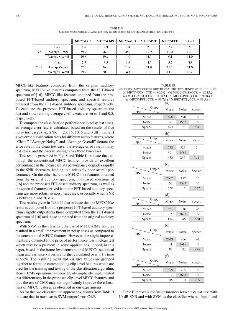
TABLE IISPEECH/MUSIC/NOISE CLASSIFICATION ERROR RATES OF DIFFERENT AUDIO FEATURES (%)

MFCC-like features computed from the original auditoryspectrum, MFCC-like features computed from the FFT-basedspectrum of [16], MFCC-like features obtained from the pro-posed FFT-based auditory spectrum, and spectral featuresobtained from the FFT-based auditory spectrum, respectively.To calculate the proposed FFT-based auditory spectrum, thefast and slow running average coefficients are set to 1 and 0.5,respectively.

To compare the classification performance in noisy test cases,an average error rate is calculated based on the results of fivenoisy test cases (i.e., SNR 20, 15, 10, 5 and 0 dB). Table IIgives error classification rates for different audio features, where“Clean,” “Average-Noisy,” and “Average-Overall” denote theerror rate in the clean test case, the average error rate in noisytest cases, and the overall average over these two cases.

Test results presented in Fig. 8 and Table II indicate that, al-though the conventional MFCC features provide an excellentperformance in the clean case, its performance degrades rapidlyas the SNR decreases, leading to a relatively poor overall per-formance. On the other hand, the MFCC-like features obtainedfrom the original auditory spectrum, FFT-based spectrum of[16] and the proposed FFT-based auditory spectrum, as well asthe spectral features derived from the FFT-based auditory spec-trum are more robust in noisy test cases, especially when SNRis between 5 and 20 dB.

Test results given in Table II also indicate that the MFCC-likefeatures computed from the proposed FFT-based auditory spec-trum slightly outperform those computed from the FFT-basedspectrum of [16] and those computed from the original auditoryspectrum.

With SVM as the classifier, the use of MFCC-CMS featuresresulted in a small improvement in noisy cases as compared tothe conventional MFCC features. However, the slight improve-ments are obtained at the price of performance loss in clean testwhich may be a problem in some applications. Indeed, in thispaper, based on the frame-level conventional MFCCs, statisticalmean and variance values are further calculated over a 1-s timewindow. The resulting mean and variance values are groupedtogether to form the corresponding clip-level features which areused for the training and testing of the classification algorithm.Hence, CMS operation has been already implicitly implementedin a different way in the proposed clip-level MFCC features, andthus the use of CMS may not significantly improve the robust-ness of MFCC features as observed in our experiments.

As for the two classification approaches, results from Table IIindicate that in most cases SVM outperforms C4.5.

TABLE IIICONFUSION MATRICES FOR DIFFERENT AUDIO FEATURE SETS AT SNR = 10 dB.

(a) MFCC-CON (CCR = 60.5%). (b) MFCC-CMS (CCR = 62.1%).(c) MFCC-AUD (CCR = 87.0%). (d) MFCC-PRE (CCR = 90.8%).

(e) MFCC-FFT (CCR = 93.7%). (f) SPEC-FFT (CCR = 89.5%)

Table III presents confusion matrices for a noisy test case with10-dB SNR and with SVM as the classifier where “Input” and



Fig. 9. MFCC/MFCC-like features for a 1-s speech clip in clean case and in noisy case with 15-dB SNR. (a) Conventional MFCC features. (b) MFCC-like featurescomputed from the proposed FFT-based auditory spectrum.

Fig. 10. MFCC/MFCC-like features for a 1-s music clip in clean case and in noisy case with 15-dB SNR. (a) Conventional MFCC features. (b) MFCC-like featurescomputed from the proposed FFT-based auditory spectrum.

“Output” represent the input audio types and the output classifi-cation decisions, respectively. Shown in Table III are the num-bers of decisions on a 1-s basis. The correct classification rate(CCR) for each feature set is given in the table caption. It is seenthat features computed from the original auditory spectrum, theFFT-based spectrum of [16], and the proposed FFT-based au-ditory spectrum generally lead to a better classification perfor-mance of the three audio categories. The low overall classifica-tion rates of the conventional MFCC features and MFCC-CMSfeatures [60.5% from Table III(a) and 62.1% from Table III(b),respectively] are due in a large part to the low proportion ofspeech samples correctly identified. In contrast, for the MFCC-like features computed from the proposed FFT-based auditoryspectrum [Table III(e)], the proportion of correctly identifiedsamples is high for all three classes, i.e., speech, music, andnoise.

Two examples of clip-level MFCC/MFCC-like features,i.e., absolute mean and variance values over a 1-s window,are given in Figs. 9 and 10 (in relative values). Fig. 9 showsthe conventional MFCC features and the MFCC-like features

computed from the proposed FFT-based auditory spectrumfor a 1-s speech clip in clean test case and in noisy test casewith 15-dB SNR. At SNR 15 dB, the MFCC-like featurescomputed from the proposed FFT-based auditory spectrum areclose to that in the clean test case. However, this is not so for theconventional MFCC features wherein the change is relativelylarge. A similar situation can be found in Fig. 10 which showsresults for a 1-s music clip. The results shown in Figs. 9 and 10demonstrate the noise robustness of the proposed FFT-basedauditory spectrum.

B. Experiments Using 8-kHz Audio Database

To further evaluate the performance of the proposed FFT-based auditory spectrum in a narrow-band application wherethe main focus is on the identification of noise, noise/nonnoiseclassification tests are conducted using 8-kHz audio databaseand with SVM as the classifier wherein nonnoise samples in-clude speech and music clips. Error classification rates of theconventional MFCC features and the MFCC-like features de-rived from the proposed FFT-based auditory spectrum are listed



TABLE IVNOISE/NONNOISE CLASSIFICATION ERROR RATES

WITH SVM AS THE CLASSIFIER (%)

TABLE VERROR CLASSIFICATION RATES OF MFCC-LIKE FEATURES COMPUTED FROM

THE PROPOSED FFT-BASED AUDITORY SPECTRUM WITH DIFFERENT

RUNNING AVERAGE COEFFICIENTS (%)

in Table IV, where the decisions are made using both 1-s and5-s clip lengths. As for the calculation of the proposed FFT-based auditory spectrum, a 512-point FFT is now used for 8-kHzsamples. Hence, the outputs from (15) are same as those with16-kHz sampling frequency and using a 1024-point FFT. There-fore, power spectrum selection can be conducted using Table Ias before except that we now only consider frequency compo-nents within 0–4 kHz range instead of 0–8 kHz. Accordingly,the dimension of the proposed self-normalized FFT-based au-ditory spectrum vector is now 96 as compared to 120 in case of16-kHz sampling frequency.

Results in Table IV shows the ability of the two sets of fea-tures in discriminating noise from nonnoise samples. These re-sults also confirm the noise robustness of the proposed FFTspectrum-based MFCC-like features as compared to the conven-tional MFCC features. Meanwhile, as the length of audio clipincreases from one second to five seconds, the proposed FFTspectrum-based MFCC-like features achieve a relatively largeimprovement in performance as compared to the conventionalMFCC features.

C. Effect of Running Average Coefficients

As mentioned in Section IV, the proposed running averagescheme is easier to use than the implementation in [16] sincethere are only two parameters to adjust. To see how differentrunning average coefficients in (17) affect the performance ofthe proposed FFT-based auditory spectrum, we carry out testsusing different coefficients wherein the fast running averagecoefficients are simply set to 1, and the slow running averagecoefficients are set to 0.5, 0.1, and 0.05, respectively. UsingMFCC-like features and SVM algorithm, test results fromspeech/music/noise classification using 16-kHz database arelisted in Table V. Results in Table V indicate that, as the slowrunning average coefficient increases, the corresponding per-formance in clean test case is improved, while the performancein noisy test cases (with 10- or 0-dB SNR) degrades. Here, theuse of a relatively small coefficient for the slow running average

leads to a relatively large increase in the ratio of spectral peakto valley, which on the one hand improves the robustness, buton the other hand may reduce the interclass difference to someextent, and thus degrades the performance in the clean test.

D. Computational Complexity

Besides the robustness to noise, an additional advantage ofthe proposed auditory-inspired FFT-based spectrum lies in itslow computational complexity. An estimation of the computa-tional load for the original auditory spectrum and the proposedFFT-based auditory spectrum is obtained by measuring the cor-responding running time.

The implementation platform is a general PC with CPU IntelP4 (3.2 GHz). The EA model and the proposed FFT-based au-ditory spectrum are implemented using Matlab. Results are ob-tained using the 16-kHz database. Corresponding to a 1-s audioinput clip, the time used for the calculation of the original au-ditory spectrum and that of the proposed FFT-based auditoryspectrum are around 1.07 and 0.08 s, respectively. Instead of theactual processing time, the comparative performance may makemore sense in this case, i.e., compared to the original auditoryspectrum, the reduction in the processing time of the proposedFFT-based auditory spectrum is more than a factor of 10.

VII. CONCLUSION

In this paper, a stochastic analysis on the noise-suppressionproperty of an EA model [17] has been presented. We havederived a closed-form expression for the auditory spectrumby using Gaussian CDF as an approximation to the originalsigmoid compression function. Inspired by the EA model, wehave presented an improved implementation for the calculationof an FFT-based auditory spectrum which allows flexibility inthe extraction of noise-robust audio features. To evaluate theperformance of the proposed FFT-based auditory spectrum, aspeech/music/noise classification task was conducted whereinSVM and C4.5 algorithms are used as the classifiers.Compared to the conventional MFCC features, the MFCC-likefeatures computed from the original auditory spectrum, andboth the MFCC-like and spectral features computed from theproposed FFT-based auditory spectrum show more robustperformance in noisy test cases. Test results also indicate that,using the new MFCC-like features, the performance of theproposed FFT-based auditory spectrum is slightly better thanthat of the original auditory spectrum, while the computationalcomplexity is reduced by an order of magnitude. The robust-ness of the MFCC-like features computed from the proposedFFT-based auditory spectrum was further confirmed by testresults of noise/nonnoise classification experiments.

APPENDIX ICLOSED-FORM EXPRESSION OF

Assume random variables and are jointly normal withzero mean and standard deviation and , respectively. Ac-cordingly, the conditional distribution function of given

, , is also normal with mean andvariance , where represents the correlationcoefficient between and [21], [22].



To facilitate the analysis, we first define the following quan-tities:

(24)

(25)

With the above assumptions about the distributions ofand , and the conditional distribution of given ,

in (3) is calculated as follows:

(26)

Therefore, (3) can be rewritten as

(27)

where and are calculated as follows:

(28)

Define

(29)

Then

(30)

As for , we have

(31)

Define

(32)

By using partial integration, we have the following result for :

(33)

Therefore, the closed-form expression of (3) is

(34)

REFERENCES

[1] J. Saunders, “Real-time discrimination of broadcast speech/music,” inProc. IEEE Int. Conf. Acoust., Speech, Signal Process., May 1996, vol.2, pp. 993–996.

[2] E. Scheirer and M. Slaney, “Construction and evaluation of a robustmultifeature speech/music discriminator,” in Proc. IEEE Int. Conf.Acoust., Speech, Signal Process., Apr. 1997, vol. 2, pp. 1331–1334.

[3] R.-Y. Qiao, “Mixed wideband speech and music coding using a speech/music discriminator,” in Proc. IEEE Region 10 Annu. Conf. SpeechImage Technol. for Comput. Telecomm., Dec. 1997, vol. 2, pp. 605–608.

[4] L. Tancerel, S. Ragot, V. T. Ruoppila, and R. Lefebvre, “Combinedspeech and audio coding by discrimination,” in Proc. IEEE WorkshopSpeech Coding, Sep. 2000, pp. 154–156.

[5] E. Wold, T. Blum, D. Keislar, and J. Wheaten, “Content-based classi-fication, search, and retrieval of audio,” IEEE Multimedia, vol. 3, no.3, pp. 27–36, Fall, 1996.

[6] T. Zhang and C.-C. J. Kuo, “Hierarchical classification of audio datafor archiving and retrieving,” in Proc. IEEE Int. Conf. Acoust., Speech,Signal Process., Mar. 1999, vol. 6, pp. 3001–3004.

[7] L. Lu, H.-J. Zhang, and H. Jiang, “Content analysis for audio classifi-cation and segmentation,” IEEE Trans. Speech Audio Process., vol. 10,no. 7, pp. 504–516, Oct. 2002.

[8] R. Cai, L. Lu, H.-J. Zhang, and L.-H. Cai, “Highlight sound effectsdetection in audio stream,” in Proc. Int. Conf. Multimedia Expo, Jul.2003, vol. 3, pp. 37–40.

[9] M. Zhao, J. Bu, and C. Chen, “Audio and video combined for homevideo abstraction,” in Proc. IEEE Int. Conf. Acoust., Speech, SignalProcess., Apr. 2003, vol. 5, pp. 620–623.

[10] T. Zhang and C.-C. J. Kuo, “Audio content analysis for online audiovi-sual data segmentation and classification,” IEEE Trans. Speech AudioProcess., vol. 9, no. 4, pp. 441–457, May 2001.

[11] G. Lu and T. Hankinson, “An investigation of automatic audio clas-sification and segmentation,” in Proc. IEEE Int. Conf. Signal Process,Aug. 2000, vol. 2, pp. 776–781.

[12] S. Kiranyaz, A. F. Qureshi, and M. Gabbouj, “A generic audio clas-sification and segmentation approach for multimedia indexing and re-trieval,” IEEE Trans. Audio, Speech, Lang. Process., vol. 14, no. 3, pp.1062–1081, May 2006.

[13] S. Ravindran and D. Anderson, “Low-power audio classification forubiquitous sensor networks,” in Proc. IEEE Int. Conf. Acoust., Speech,Signal Process., May 2004, vol. 4, pp. 337–340.

[14] N. Mesgarani, S. Shamma, and M. Slaney, “Speech discriminationbased on multiscale spectro–temporal modulations,” in Proc. IEEEInt. Conf. Acoust., Speech, Signal Process., May 2004, vol. 1, pp.601–604.

[15] W. Chu and B. Champagne, “A simplified early auditory model withapplication in speech/music classification,” in Proc. IEEE Can. Conf.Elect. Comput. Eng., May 2006, pp. 578–581.

[16] W. Chu and B. Champagne, “A noise-robust FFT-based spectrum foraudio classification,” in Proc. IEEE Int. Conf. Acoust., Speech, SignalProcess., May 2006, vol. 5, pp. 213–216.

[17] K. Wang and S. Shamma, “Self-normalization and noise-robustness inearly auditory representations,” IEEE Trans. Speech Audio Process.,vol. 2, no. 3, pp. 421–435, Jul. 1994.

[18] J. R. Quinlan, C4.5:Programs for Machine Learning. San Mateo,CA: Morgan Kaufmann, 1993.

[19] M. Elhilali, T. Chi, and S. Shamma, “A spectro–temporal modula-tion index (STMI) for assessment of speech intelligibility,” SpeechCommun., vol. 41, pp. 331–348, Oct. 2003.



[20] Neural Syst. Lab., Univ. Maryland, “NSL Matlab Toolbox.” [Online].Available: http://www.isr.umd.edu/Labs/NSL/nsl.html.

[21] A. Papoulis and S. U. Pillai, Probability, Random Variables, and Sto-chastic Processes, 4th ed. New York: McGraw-Hill, 2002.

[22] P. L. Meyer, Introductory Probability and Statistical Applications, 2nded. Reading, MA: Addison-Wesley, 1970.

[23] P.-W. Ru, “Perception-based multi-resolution auditory processing ofacoustic signals,” Ph.D. dissertation, Univ. Maryland, College Park,2000.

[24] D. O’Shaughnessy, Speech Communications-Human and Machines,2nd ed. New York: IEEE Press, 2000.

[25] M. Slaney, “Auditory Toolbox: A Matlab Toolbox for Auditory Mod-eling Work (Version 2),” Interval Research Corp., Tech. Rep. 1998-010,1998 [Online]. Available: http://www.slaney.org/malcolm/pubs.html.

[26] B. S. Atal, “Effectiveness of linear prediction characteristics of thespeech wave for automatic speaker identification and verification,” J.Acoust. Soc. Amer., vol. 55, no. 6, pp. 1304–1312, Jun. 1974.

[27] C. Xu, N. C. Maddage, and X. Shao, “Automatic music classificationand summarization,” IEEE Trans. Speech Audio Process., vol. 13, no.3, pp. 441–450, May 2005.

[28] S. Z. Li, “Content-based audio classification and retrieval using thenearest feature line method,” IEEE Trans. Speech Audio Process., vol.8, no. 5, pp. 619–625, Sep. 2000.

[29] A. Varga, H. J. M. Steeneken, M. Tomlinson, and D. Jones, “TheNOISEX-92 study on the effect of additive noise on automatic speechrecognition,” 1992, documentation included in the NOISEX-92CD-ROMs.

[30] TDMA Cellular/PCS-Radio Interface-Minimum Performance Stan-dards for Discontinuous Transmission Operation of Mobile Stations,TIA/EIA/IS-727, Jun. 1998.

[31] I. Tsochantaridis, T. Joachims, T. Hofmann, and Y. Altun, “Largemargin methods for structured and interdependent output variables,”J. Mach. Learn. Res. vol. 6, pp. 1453–1484, Sep. 2005 [Online].Available: http://svmlight.joachims.org/svm_struct.html.

[32] Y. Li and C. Dorai, “SVM-based audio classification for instructionalvideo analysis,” in Proc. IEEE Int. Conf. Acoust., Speech, SignalProcess., May 2004, vol. 5, pp. 897–900.

Wei Chu received the B.E. and M.E. degrees fromHefei University of Technology, Hefei, China, andthe M.A.Sc. degree from Concordia University, Mon-tréal, QC, Canada. He is currently pursuing the Ph.D.degree in the Department of Electrical and ComputerEngineering, McGill University, Montréal.

His research interests are in the area of speech andaudio signal processing, including content-basedaudio analysis, noise suppression, speech detection,speech/audio compression, and real-time DSPimplementation of speech/audio algorithms.

Benoît Champagne was born in Joliette, QC,Canada, in 1961. He received the B.Ing. degreein engineering physics from École Polytechnique,Montréal, QC, Canada, in 1983, the M.Sc. degreein physics from Université de Montréal in 1985,and the Ph.D. degree in electrical engineering fromthe University of Toronto, Toronto, ON, Canada, in1990.

From 1990 to 1999, he was an Assistant and thenAssociate Professor at INRS-Télécommunications,Université du Québec, Montréal, where he is cur-

rently a Visiting Professor. In September 1999, he joined McGill University,Montréal, as an Associate Professor within the Department of Electrical andComputer Engineering, where he is currently acting as Associate Chairmanof Graduate Studies. His research interests lie in the area of statistical signalprocessing, including signal/parameter estimation, sensor array processing, andadaptive filtering and applications thereof to communications systems.


IEEE TRANSACTIONS ON AUDIO, SPEECH, AND …bchamp/Papers/Jounal/IEEE-ASLP2008.pdfthis manuscript and...

Documents

Transcript of IEEE TRANSACTIONS ON AUDIO, SPEECH, AND …bchamp/Papers/Jounal/IEEE-ASLP2008.pdfthis manuscript and...