Computationally E cient Approaches for Blind Adaptive Beamforming...

Computationally Efficient Approaches forBlind Adaptive Beamforming in

SIMO-OFDM Systems

Bo Gao

Department of Electrical & Computer EngineeringMcGill UniversityMontreal, Canada

May 2009

A thesis submitted to McGill University in partial fulfillment of the requirements for thedegree of Master.

c© 2009 Bo Gao

i

Abstract

In single-input multiple-output (SIMO) systems based on orthogonal frequency division

multiplexing (OFDM), adaptive beamforming at the receiver side can be used to combat

the effect of directional co-channel interference (CCI). Since pilot-aided beamforming suf-

fers from consuming precious channel bandwidth, there has been much interest in blind

beamforming approaches that can adapt their weights by restoring certain properties of

the transmitted signals. Within this class of blind algorithms, the recursive least squares

constant modulus algorithm (RLS-CMA) is of particular interest due to its good overall

CCI cancelation performance and fast convergence. Nevertheless, the direct use of RSL-

CMA within a SIMO-OFDM receiver induces considerable computational complexity, since

a distinct copy of the RLS-CMA must be run on each individual sub-carriers. In this the-

sis, we present two approaches to reduce the computational complexity of SIMO-OFDM

beamforming based on the RLS-CMA, namely: frequency interpolation and distributed

processing. The former approach, which exploits the coherence bandwidth of the broad-

band wireless channels, divides the sub-carriers into several contiguous groups and applies

the RLS-CMA to a selected sub-carrier in each group. The weight vectors at other frequen-

cies are then obtained by interpolation. The distributed processing approach relies on the

partitioning of the receiving array into sub-arrays and the use of a special approximation

in the RLS-CMA. This allows a partial decoupling of the algorithm which can then be run

on multiple processors with reduced overall complexity. This approach is well-suited to col-

laborative beamforming in multi-node distributed relaying. Through numerical simulation

experiments of a SIMO-OFDM system, it is demonstrated that the proposed modifications

to the RLS-CMA scheme can lead to substantial computational savings with minimal losses

in adaptive cancelation performance.

ii

Resume

Dans les systemes a une entree et a multiples sorties (SIMO, soit single-input multiple

output) bases sur le multiplexage par repartition orthogonale de la frequence (OFDM,

soit orthogonal frequency division multiplexing), la formation de faisceaux adaptatifs du

cote du recepteur peut etre utilisee pour combattre l’effet de brouillage directionnel a

l’interieur d’un meme canal. Puisque la formation de faisceaux a l’aide de pilotes presente

l’inconvenient d’utiliser la bande passante convoitee des canaux, il existe beaucoup d’interet

pour les approches aveugles de formation de faisceaux qui peuvent adapter leurs poids en

restaurant certaines proprietes des signaux transmis. Parmi cette classe d’algorithmes

aveugles, l’algorithme a module constant suivant la methode des moindres carres recursive

(RLS-CMA, soit recursive least squares constant modulus algorithm) presente un interet

particulier de par son efficacite globale d’elimination de brouillage dans un meme canal et

sa convergence rapide. Neanmoins, l’utilisation directe d’un RLS-CMA dans un recepteur

SIMO-OFDM cree une complexite informatique considerable, puisqu’il faut executer une

copie distincte du RLS-CMA dans chaque sous-porteuse individuelle. Dans la presente

these, nous presenterons deux approches pour reduire la complexite informatique de la for-

mation de faisceaux SIMO-OFDM basee sur le RLS-CMA : l’interpolation des frequences et

le traitement reparti. La premiere approche, qui exploite la largeur de bande de coherence

des canaux sans fil a large bande, divise les sous-porteuses en plusieurs groupes contigus

et applique le RLS-CMA a une sous-porteuse choisie dans chaque groupe. Les vecteurs de

poids aux autres frequences sont alors obtenus par interpolation. L’approche par traite-

ment reparti est basee sur le partitionnement du reseau de reception en sous-reseaux et sur

l’utilisation d’une approximation speciale dans le RLS-CMA. Cela permet un decouplage

partiel de l’algorithme, qui peut alors etre execute sur de multiples processeurs en reduisant

la complexite globale. Cette approche est bien adaptee a la formation de faisceaux en col-

laboration dans les systemes multi-noeuds a relais distribues. Grace a des experiences

de simulation numerique d’un systeme SIMO-OFDM, nous demontrons que les modifica-

tions proposees au schema RLS-CMA peuvent mener a des economies informatiques non

negligeables avec des pertes minimes dans l’elimination adaptative du brouillage.

iii

Acknowledgments

I have been studying for two and half years in the permit of my master’s degree in electrical

engineering. During this period of time, I have learnt both academic knowledge and a

positive living attitude. With my supervisor, parents and friends’ help, I have completed

my master’s research, and finally have a chance to give my appreciation to all of you.

First, I would like to thank my supervisor Dr. Champagne. He was the one, who

directed me to follow the right research track and avoid losing precious time. He was

always supportive to give advice, and showed me the method and attitude to face new

problems. I had some difficult time during my study, without his help, I could not make

this far.

Secondly, I should say thank you to my parents. Same as most of the parents, their

love to me is selfless. Since I am the only child in my family, they have done the most they

could to create the best growing up environment only for me. I want to thank them for

both their moral influence, and economic support. I would like to give this thesis report as

a gift to them.

Finally, I show great appreciation to my girlfriend, Yinan Xu, and all others, who were

companying me during the past two years. Your help will always be remembered.

iv

Contents

1 Introduction 1

1.1 Literature Review on Blind Adaptive Beamforming . . . . . . . . . . . . . 3

1.2 Problem Addressed and Motivation . . . . . . . . . . . . . . . . . . . . . . 4

1.3 Thesis Contribution . . . . . . . . . . . . . . . . . . . . . . . . . . . . . . . 4

1.3.1 Interpolation . . . . . . . . . . . . . . . . . . . . . . . . . . . . . . 4

1.3.2 Distributed Processing . . . . . . . . . . . . . . . . . . . . . . . . . 5

1.4 Thesis Organization . . . . . . . . . . . . . . . . . . . . . . . . . . . . . . . 6

2 Adaptive Beamforming 7

2.1 Basic Concepts . . . . . . . . . . . . . . . . . . . . . . . . . . . . . . . . . 7

2.1.1 Uniform Linear Array (ULA) . . . . . . . . . . . . . . . . . . . . . 8

2.1.2 Fixed Beamforming . . . . . . . . . . . . . . . . . . . . . . . . . . . 8

2.1.3 Adaptive beamforming . . . . . . . . . . . . . . . . . . . . . . . . . 10

2.2 Non-Blind Adaptive Beamforming . . . . . . . . . . . . . . . . . . . . . . . 11

2.2.1 Least Mean Square (LMS) Algorithm . . . . . . . . . . . . . . . . . 11

2.2.2 Recursive Least Squares (RLS) Algorithm . . . . . . . . . . . . . . 14

2.3 Blind Adaptive Beamforming . . . . . . . . . . . . . . . . . . . . . . . . . 16

2.3.1 LMS-based CMA . . . . . . . . . . . . . . . . . . . . . . . . . . . . 16

2.3.2 RLS-CMA . . . . . . . . . . . . . . . . . . . . . . . . . . . . . . . . 17

2.4 Chapter Summary . . . . . . . . . . . . . . . . . . . . . . . . . . . . . . . 20

3 OFDM and System Model 22

3.1 OFDM . . . . . . . . . . . . . . . . . . . . . . . . . . . . . . . . . . . . . . 22

3.1.1 Orthogonality . . . . . . . . . . . . . . . . . . . . . . . . . . . . . . 23

3.1.2 Baseband OFDM Configuration . . . . . . . . . . . . . . . . . . . . 25

Contents v

3.1.3 Cyclic Prefix (CP) . . . . . . . . . . . . . . . . . . . . . . . . . . . 26

3.2 SIMO-OFDM System Model . . . . . . . . . . . . . . . . . . . . . . . . . . 28

3.2.1 System Configuration . . . . . . . . . . . . . . . . . . . . . . . . . . 28

3.2.2 System Performance . . . . . . . . . . . . . . . . . . . . . . . . . . 29

3.3 Chapter Summary . . . . . . . . . . . . . . . . . . . . . . . . . . . . . . . 32

4 Reduction of System Complexity 34

4.1 Interpolation . . . . . . . . . . . . . . . . . . . . . . . . . . . . . . . . . . 34

4.1.1 DFT-based Interpolation . . . . . . . . . . . . . . . . . . . . . . . . 35

4.1.2 Flat-top Interpolation . . . . . . . . . . . . . . . . . . . . . . . . . 36

4.1.3 Linear Interpolation . . . . . . . . . . . . . . . . . . . . . . . . . . 37

4.1.4 Complexity Reduction . . . . . . . . . . . . . . . . . . . . . . . . . 40

4.2 Distributed Processing . . . . . . . . . . . . . . . . . . . . . . . . . . . . . 42

4.2.1 Algorithm Derivation . . . . . . . . . . . . . . . . . . . . . . . . . . 43

4.2.2 Complexity Reduction . . . . . . . . . . . . . . . . . . . . . . . . . 46

4.3 Chapter Summary . . . . . . . . . . . . . . . . . . . . . . . . . . . . . . . 48

5 Simulation Results and Discussion 49

5.1 Simulation Parameters and Channel Model . . . . . . . . . . . . . . . . . . 49

5.1.1 System Parameters . . . . . . . . . . . . . . . . . . . . . . . . . . . 50

5.1.2 Channel Model . . . . . . . . . . . . . . . . . . . . . . . . . . . . . 50

5.1.3 Performance Measure . . . . . . . . . . . . . . . . . . . . . . . . . . 51

5.2 Interpolation Methods . . . . . . . . . . . . . . . . . . . . . . . . . . . . . 52

5.3 Distributed Processing . . . . . . . . . . . . . . . . . . . . . . . . . . . . . 57

5.4 Combining Both Approaches . . . . . . . . . . . . . . . . . . . . . . . . . . 61

5.5 Chapter Summary . . . . . . . . . . . . . . . . . . . . . . . . . . . . . . . 64

6 Conclusion and Future Work 65

6.1 Thesis Overview . . . . . . . . . . . . . . . . . . . . . . . . . . . . . . . . . 65

6.2 Main Contributions . . . . . . . . . . . . . . . . . . . . . . . . . . . . . . . 66

6.3 Future Research Direction . . . . . . . . . . . . . . . . . . . . . . . . . . . 67

References 68

Contents vi

A Raw data for Figure 5.10 71

vii

List of Figures

1.1 Simple SIMO configuration for wireless communication. . . . . . . . . . . . 2

2.1 Uniform Linear Array (ULA). . . . . . . . . . . . . . . . . . . . . . . . . . 8

2.2 Beamforming Structure. . . . . . . . . . . . . . . . . . . . . . . . . . . . . 9

2.3 Original beampattern (all weights set to 1). . . . . . . . . . . . . . . . . . 10

2.4 Beampattern for steering direction of θ = 10◦. . . . . . . . . . . . . . . . . 10

2.5 Adaptive Beamforming Structure. . . . . . . . . . . . . . . . . . . . . . . . 11

2.6 Beampattern after convergence (top) and SINR versus iteration (bottom)

for the LMS algorithm with different values of the step size µ. . . . . . . . 13

2.7 Beampattern after convergence (top) and SINR versus iteration (bottom)

for the LMS and the RLS algorithm. . . . . . . . . . . . . . . . . . . . . . 15

2.8 Constellation of the received symbols before and after the phase rotation. . 18

2.9 Beampattern after convergence (top) and SINR (bottom) versus iteration

for the LMS-CMA and the RLS-CMA. . . . . . . . . . . . . . . . . . . . . 20

2.10 Re-convergence ability of the LMS-CMA and the RLS-CMA. . . . . . . . 21

3.1 Combining OFDM sub-carriers. . . . . . . . . . . . . . . . . . . . . . . . . 24

3.2 Baseband OFDM model. . . . . . . . . . . . . . . . . . . . . . . . . . . . . 25

3.3 ISI elimination by adding silent GI to OFDM time domain symbols. . . . . 27

3.4 Cyclic Prefix. . . . . . . . . . . . . . . . . . . . . . . . . . . . . . . . . . . 27

3.5 Baseband SIMO-OFDM model. . . . . . . . . . . . . . . . . . . . . . . . . 30

3.6 Simplified frequency selective channel. . . . . . . . . . . . . . . . . . . . . 31

3.7 Beampatterns obtained with the RLS-CMA in SIMO-OFDM system for all

sub-carriers. . . . . . . . . . . . . . . . . . . . . . . . . . . . . . . . . . . . 32

List of Figures viii

4.1 Coherence bandwith versus OFDM sub-carriers. . . . . . . . . . . . . . . . 35

4.2 Select OFDM sub-carriers into groups. . . . . . . . . . . . . . . . . . . . . 35

4.3 Flat-top interpolation. . . . . . . . . . . . . . . . . . . . . . . . . . . . . . 36

4.4 Linear interpolation. . . . . . . . . . . . . . . . . . . . . . . . . . . . . . . 38

4.5 Linear interpolation with phase error in the complex plane. . . . . . . . . . 39

4.6 Interpolation with phase-rotation. . . . . . . . . . . . . . . . . . . . . . . . 40

4.7 Collaborative beamforming: Q sub-arrays, each equipped with L antennas. 43

4.8 Block diagram of distributed RLS-CMA. . . . . . . . . . . . . . . . . . . . 47

5.1 Illustrative realization of the Rayleigh fading channel. . . . . . . . . . . . . 51

5.2 Average SINR versus iteration number for flat-top interpolation. . . . . . . 54

5.3 Average SINR versus iteration number for linear interpolation. . . . . . . . 54

5.4 Steady-state sub-carrier SINR versus frequency index for flat-top interpolation. 55

5.5 Steady-state sub-carrier SINR versus frequency index for linear interpolation. 55

5.6 BER of SIMO-OFDM beamforming based on RLS-CMA with flat-top inter-

polation. . . . . . . . . . . . . . . . . . . . . . . . . . . . . . . . . . . . . . 56

5.7 BER of SIMO-OFDM beamforming based on RLS-CMA with linear inter-

polation. . . . . . . . . . . . . . . . . . . . . . . . . . . . . . . . . . . . . . 57

5.8 Array partitions used for evaluation of the the distributed processing scheme. 58

5.9 Comparing average SINR for RLS-CMA based on different sub-array distri-

butions (same λ = 0.98 for all configurations). . . . . . . . . . . . . . . . . 59

5.10 Steady-state SINR of three different array distributions verses their corre-

sponding initial convergence slope. . . . . . . . . . . . . . . . . . . . . . . 60

5.11 Comparing average SINR on all sub-carriers for different sub-array distribu-

tions with different values of λ. . . . . . . . . . . . . . . . . . . . . . . . . 61

5.12 Comparing BER performance of RLS-CMA based SIMO-OFDM beamform-

ing for different sub-array distributions (same λ = 0.98 for all configurations). 62

5.13 Comparing average SINR on all sub-carriers of combined scheme with the

original algorithm (λ = 0.98). . . . . . . . . . . . . . . . . . . . . . . . . . 63

5.14 Comparing BER of RLS-CMA based SIMO-OFDM beamforming of com-

bined scheme with the original algorithm (λ = 0.98). . . . . . . . . . . . . 63

ix

List of Tables

4.1 Summary of the distributed RLS-CMA . . . . . . . . . . . . . . . . . . . . 46

5.1 Computational complexity of interpolated RLS-CMA. . . . . . . . . . . . . 52

5.2 Computation complexity of distributed processing. . . . . . . . . . . . . . . 58

A.1 (10)-element array . . . . . . . . . . . . . . . . . . . . . . . . . . . . . . . 71

A.2 (5,5)-element array . . . . . . . . . . . . . . . . . . . . . . . . . . . . . . . 71

A.3 (3,3,4)-element array . . . . . . . . . . . . . . . . . . . . . . . . . . . . . . 71

x

List of Acronyms

SIMO Single-Input Multiple-Output

MIMO Multiple-Input Multiple-Output

OFDM Orthogonal Frequency Division Multiplexing

CP Cyclic Prefix

CCI Co-Channel Interference

ISI Inter Symbol Interference

ICI Inter Carrier Interference

FM Frequency Modulation

PM Phase Modulation

BPSK Binary Phase Shift Key

QAM Quadrature Amplitude Modulation

ULA Uniform Linear Array

AF Array Factor

AV Array Vector

AOA Angle Of Arrival

CMA Constant Modulus Algorithm

LMS Least Mean Square

SD Steepest Descent

RLS Recursive Least Squares

LS Least Squares

rms root mean square

SNR Signal to Noise Ratio

SINR Signal to Interference and Noise Ratio

BER Bit Error Rate

List of Terms xi

DFT discrete Fourier Mransform

FFT Fast Fourier Mransform

IFFT Inverse Fast Fourier Transform

AWGN Additive White Gaussian Noise

TX Transmitter

RX Receiver

MVDR minimum-variance distortionless response

1

Chapter 1

Introduction

Today’s increasing demand for high data rate transmissions continues to spur the search

of improved signal processing techniques for wideband wireless communication systems.

Consideration of fundamental issues in the design of these systems, such as the frequency

selective fading due to multipath propagation and receiver complexity, naturally leads to

the use of orthogonal frequency division multiplexing (OFDM) techniques.

OFDM splits the wideband channel into a number of sub-channels with smaller band-

width, so that each sub-channel is experiencing near flat fading [1, 2, 3]. As a multi-carrier

modulation technique, OFDM converts single high speed data stream into multiple low

speed data streams, and modulates them onto different sub-carriers. These parallel sub-

carriers are allocated as close to each other as possible without breaking the orthogonality

among them. As a result, OFDM is very spectrum efficient. The frequency selective prop-

erty of the dispersive radio environment is characterized by its delay spread, or coherence

bandwidth, which is proportional to the inverse of the rms delay spread [4]. The smaller

the coherence bandwidth, the more frequency selective the channel is. Hence, by choos-

ing a reasonable spacing between sub-carrier corresponding to the coherence bandwidth,

the original frequency selective channel can be approximated as a number of multiple and

independent parallel flat channels; and by adding cyclic prefix (CP), instead of a silent

guard period, inter symbol interference (ISI) is completely eliminated without losing the

orthogonality of the OFDM and producing the inter carrier interference (ICI)1, as long as

the CP is larger than the delay spread [5]. Therefore, OFDM considerably simplifies the

1ICI is crosstalk between different sub-carriers, which means they are no longer orthogonal

1 Introduction 2

implementation of the channel equalization.

In addition, to mitigate the effects of co-channel interference (CCI) originating from

users at different locations, an effective approach consists of using multiple antennas at

the receiver side (e.g. base-station). When the users are equipped with single-antenna

terminals, as is assumed in this work, the resulting transmission channel from the desired

user to the antenna array receiver defines a single-input multi-output (SIMO) system [1].

This situation is illustrated in Figure 1.1.

SIMO System

Fig. 1.1 Simple SIMO configuration for wireless communication.

In a SIMO-OFDM receiver, adaptive beamforming techniques can be applied indepen-

dently on each parallel OFDM sub-channel to suppress CCI. Each beamformer iteratively

computes the weights of a spatial filter so as to optimally combine the signal components

originating from the desired user while rejecting signals of the same frequency but imping-

ing upon the array from other directions. This way, the signal-to-interference-plus-noise

ratio (SINR) of the desired user at the corresponding frequency can be maximized. The

combination of OFDM and adaptive beamforming techniques for broadband communica-

tion has been studied in the literature. Reference [6] first studies the combination of OFDM

with a pilot sequence assisted algorithm for simple matrix inversion beamforming. In [7]

and [8], different blind adaptive algorithms are utilized together with the OFDM scheme.

In this thesis project, a blind adaptive algorithm, recursive least squares constant modu-

lus algorithm (RLS-CMA), will be applied to the SIMO-OFDM system, for slowly fading

channels. A general literature review of the blind beamforming techniques is presented in

the next section.

1 Introduction 3

1.1 Literature Review on Blind Adaptive Beamforming

Adaptive beamforming techniques can be implemented by using pilot (or training) se-

quences to drive the iterative weight optimization process and so form adequate beam-

patterns [9]. However, this approach requires the allocation of precious system bandwidth

which may not be available for data transmission. To overcome this limitation, there

has been much interest in blind beamforming approaches that can adapt their weights by

restoring certain properties of the transmitted signals.

Many communication signals have the constant modulus (CM) property, such as fre-

quency modulation (FM), phase modulation (PM), binary phase shift key (BPSK), and

Quadrature Amplitude Modulation (QAM). The amplitude of these signals is invariant

with changing phase or frequency. In this respect, blind techniques based on the so-called

CM criterion approach have been widely used due to their good overall CCI cancelation

performance. The key goal of the CM algorithms is to recover the CM property from the

received signals, which are corrupted by the propagation channel and interfering wave.

In recent years, various CM algorithms have been developed based on different opti-

mality and search criteria. Among these, the constant modulus algorithm (CMA), which

is based on least mean square (LMS) approach has attracted much interest. As demon-

strated in [10], the performance of the CMA strongly depends on the selected value of step

size. In [11], a least squares constant modulus algorithm (LS-CMA) is proposed based

on a least square (LS) formulation of the problem; this algorithm uses a block updating

scheme. Within the class of LS-based blind algorithms, the recursive least squares constant

modulus algorithm (RLS-CMA) is of particular interest due to its good overall CCI can-

celation performance and fast convergence. The details of RLS-CMA, which is based on

the standard RLS [9], have been presented in [12, 13], and the comparison to other blind

adaptive criteria were also established. Through the simulation results, [12] and [13] have

verified that the RLS-CMA offers the best convergence property for both cyclostationary

signals and random stationary signals respectively. In [14], more comparisons have been

made among adaptive algorithms, and the RLS-CMA was also modified to a multi-modulus

algorithm (MMA) to work for high order QAM constellations.

1 Introduction 4

1.2 Problem Addressed and Motivation

Since OFDM allows flat fading channel techniques, such as RLS-CMA, to be applied to

the broadband communication for data processing, and RLS-CMA has been proved to offer

good convergence property, the SIMO-OFDM beamforming system is suitable for the urban

dispersive mobile radio environment. Nevertheless, the direct use of RSL-CMA within a

SIMO-OFDM receiver induces considerable computational complexity. Indeed, the RLS-

CMA adaptation involves the calculation of the inverse correlation matrix of the input

data, and its complexity is of order K2, i.e. O(K2)2, where K is the length of the weight

vector. Also, a distinct copy of it must be run on each individual OFDM sub-carrier, for

a total complexity of O(NK2) per iteration, where N is the number of sub-carriers. For

instance, the IEEE 802.11a OFDM model has 48 data sub-carriers [15], and accordingly,

the RLS-CMA has to be applied 48 times individually to the system.

Since the complexity is the major issue of the SIMO-OFDM beamforming system, the

objective of this thesis is to develop methods which can mitigate this short coming. Most

of the time, complexity reduction is accompanied by a decrease in system performance

as a trade off. Therefore, the goal of the thesis is to compromise between the system

performance and the computational complexity.

1.3 Thesis Contribution

In this thesis, we propose two approaches to reduce the computational complexity of the

SIMO-OFDM beamforming system based on the RLS-CMA, namely: frequency domain

interpolation and spacial domain distributed processing.

1.3.1 Interpolation

Some interpolation-based methods to reduce the complexity of the channel estimation of the

Multiple-Input Multiple-Output (MIMO) OFDM system were developed in recent years.

For instance, [16] proposed a zero-forcing filter interpolation, by exploiting the fact that

the adjoint and the determinant of a polynomial channel matrix is still polynomial, and

2In this thesis the big big order notation O(x) = α(x)+φ(x) notation is frequently used in computationalcomplexity theory to describe how the size of the input data affects an algorithm’s usage of computationalresources (usually running time or memory), where α ∈ <+ is a constant and φ(x) is a function such thatlimx→∞

φ(x)x = 0.

1 Introduction 5

[17] utilized the DFT-based interpolation to obtain a full estimation of the channel from

reduced channel matrices in the frequency domain. In this thesis, we propose interpolation

techniques that exploit the coherence bandwidth of the broadband wireless channels. For

transmission of radio signals through highly correlated channels, the number of OFDM sub-

carriers is much larger than the channel order. Therefore, several contiguous sub-carriers

may end up experiencing similar fading conditions. This suggest that the RLS-CMA can

be applied only to several selected tones, while the weight vectors of adjacent tones are

obtained by interpolation. In the thesis, different interpolation approaches are developed

and compared. Since the calculation complexities of the proposed interpolation schemes

are much less than the RLS-CMA adaptation, and most of the weight vectors are obtained

by interpolation, the system’s complexity is decreased dramatically. Indeed if we assume

that the RLS-CMA is applied once for every m sub-carriers, the total complexity of the

system is reduced to O(NmK2) per iteration.

1.3.2 Distributed Processing

Distributed processing is also proposed to reduce the system complexity. It relies on the

partitioning of the receiving array into sub-arrays and the use of a special approximation

in the RLS-CMA. This allows a partial decoupling of the algorithm. Not only has the

resulting algorithm an overall lower complexity, but it can also be run on multiple processors

simultaneously. This approach is well-suited for collaborative beamforming in the multi-

node distributed relaying, which is developed for energy constrained sensor networks. With

this implementation, multiple sensors are able to collaboratively communicate with the base

station, by forming a directive beam [18]. If the whole antenna array is divided into M

sub-arrays, the system complexity is reduced to O(NMK2) per iteration with the proposed

distributed approach.

The two methods above can also be combined. In this case, the system complexity is

reduced due to both spatial and frequency domain processing, as O( NmM

K2). However,

this combination may have more important effect on the system performance, and different

values of m and M should be tried for the best compromise.

1 Introduction 6

1.4 Thesis Organization

The rest of the thesis is organized as follows. Chapter 2 reviews various adaptive beam-

forming techniques, and discuses their relative performance. Chapter 3 briefly reviews basic

OFDM concepts, and then presents the SIMO-OFDM system model under consideration in

this work. Chapter 4 develops the two proposed techniques for computational complexity

reduction of blind SIMO-OFDM beamforming based on RLS-CMA. Simulation results of

SIMO-OFDM transmission are shown and discussed in Chapter 5 to demonstrate the sys-

tem performance after applying these complexity reduction techniques. Finally, Chapter 6

gives a summary of the thesis, and mentions possible future work.

7

Chapter 2

Adaptive Beamforming

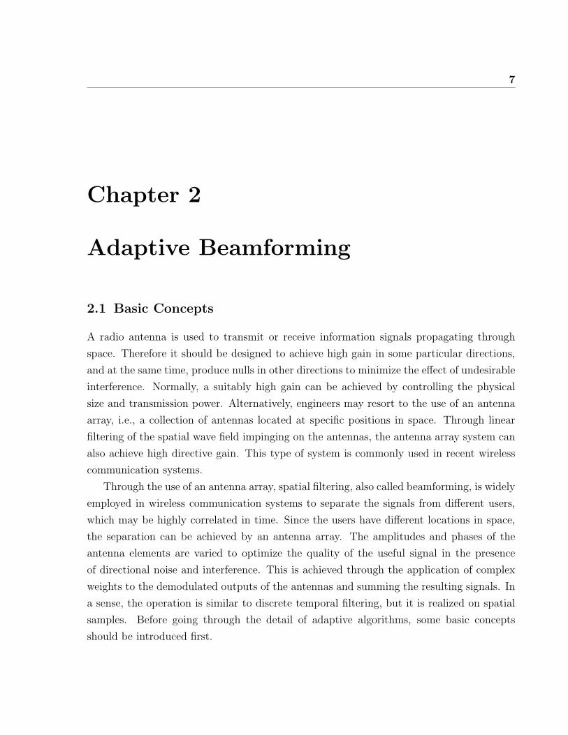
2.1 Basic Concepts

A radio antenna is used to transmit or receive information signals propagating through

space. Therefore it should be designed to achieve high gain in some particular directions,

and at the same time, produce nulls in other directions to minimize the effect of undesirable

interference. Normally, a suitably high gain can be achieved by controlling the physical

size and transmission power. Alternatively, engineers may resort to the use of an antenna

array, i.e., a collection of antennas located at specific positions in space. Through linear

filtering of the spatial wave field impinging on the antennas, the antenna array system can

also achieve high directive gain. This type of system is commonly used in recent wireless

communication systems.

Through the use of an antenna array, spatial filtering, also called beamforming, is widely

employed in wireless communication systems to separate the signals from different users,

which may be highly correlated in time. Since the users have different locations in space,

the separation can be achieved by an antenna array. The amplitudes and phases of the

antenna elements are varied to optimize the quality of the useful signal in the presence

of directional noise and interference. This is achieved through the application of complex

weights to the demodulated outputs of the antennas and summing the resulting signals. In

a sense, the operation is similar to discrete temporal filtering, but it is realized on spatial

samples. Before going through the detail of adaptive algorithms, some basic concepts

should be introduced first.


2.1.1 Uniform Linear Array (ULA)

Since different radio environments are characterized by different channel conditions, several

different types of antenna geometries have been considered. Among these, three common

types of array geometries that are encountered in applications include: the uniform linear

array (ULA), the circular array, and the planar array. The names of these arrays are

defined after their shapes. However, other geometries are possible. For example, in Ad Hoc

sensor network [18], the antenna elements are randomly distributed in a certain area to do

collaborative beamforming.

The model used in this thesis is based on a ULA, whose configuration is illustrated in

Figure 2.1. In this figure, θ is the angle of arrival (AOA) of a propagating plane signal

waveform. The same type of antennas are used in the array, and the antenna spacing, d,

between adjacent elements in a constant parameter, i.e., elements are uniformly distributed.

Typically, d = λ2

is often applied for a good compromise between unwanted mutual coupling

effects and control of ambiguity lobes, where λ is the wavelength of the transmitted signal

[19], i.e., the inverse of the carrier frequency.

Ө

dsin(Ө)

d d

Antenna elements

Signal direction Normal to

array

Fig. 2.1 Uniform Linear Array (ULA).

2.1.2 Fixed Beamforming

The array vector (AV), also called steering vector, is an important concept for beamforming.

It characterizes the number of the elements, the geometry of the array, and the amplitude

and phase of each element. When an ULA is used in the system, each element receives

the same signal but with different time delays, as represented by equivalent phase shifts.

Therefore, the received signal amplitude of each element is the same. Corresponding to


Figure 2.1, the AV is defined as

AV(θ) = [1, ejkdsin(θ), ej2kdsin(θ), . . . , ej(K−1)kdsin(θ)]T

(2.1)

where k is the steering parameter, and K is the number of the antenna elements in the

array.

The weight vector of the beamforming system is designed to adjust AV in order to

control the direction of the beampattern. The basic beamforming structure to compensate

for the phase difference in the array vector is shown in Figure 2.2, where [x1(n) · · ·xK(n)]

Sum

Sample

Sample

Sample

*

1w)(1 nx

)(2 nx

)(nxK

)(ny*

2w

*

Kw

Fig. 2.2 Beamforming Structure.

denote the baseband antenna samples at discrete-time n, wi is the complex weight applied

to the ith antenna output and y(n) is the beamforming output, given by

y(n) =K∑i=1

w∗i xi(n) (2.2)

A normalized beampattern, corresponding to weights wi = 1, is shown in Figure 2.3

for a ULA with K = 10 antennas. In this example, the polar plot gives the response, (i.e.

gain), of the beamforming system to a plane wave with AOA of θ ∈ (−90◦, 90◦). Because

of the special choice of weights, the main lob is perpendicular to the ULA. If the useful

signal has an AOA= 10◦, by changing the amplitude and phase of the weight vector, the

beampattern can be redirected to the desired direction, as shown in Figure 2.4.


0.2

0.4

0.6

0.8

1

30

210

60

240

90

270

120

300

150

330

180 0

Fig. 2.3 Original beampattern (all weights set to 1).

0.2

0.4

0.6

0.8

1

30

210

60

240

90

270

120

300

150

330

180 0

Fig. 2.4 Beampattern for steering direction of θ = 10◦.

2.1.3 Adaptive beamforming

Adaptive beamforming is based on similar principles, but instead of using a set of fixed

antenna weights, these are updated in realtime to “best match” the changing conditions of

the surrounding propagation and interference environment. This is typically achieved via

feedback control aimed at restoring the quality of the output signal, y(n). This can be done

by exploiting the statistics of the channel, a pilot of reference signals or other structural

properties. The basic adaptive beamforming structure is shown in Figure 2.5, which is

modified from Figure 2.2 by adding the feedback control algorithm into the system, and

allowing the weights to vary with time, i.e., wi(n).

For adaptive beamforming, several different methods or algorithms are available to ad-


Sum

Sample

Sample

Sample

*

1w)(1 nx

)(2 nx

)(nxK

)(ny*

2w

*

Kw

Adaptive

algorithm

Fig. 2.5 Adaptive Beamforming Structure.

just the weights, wi(n), iteratively over time as new data xi(n) become available. The

directivity of the adaptive beamforming system, represented by its beampattern, will also

change with the weights, which are adjusted at each iteration. A well designed adap-

tive beamforming system will result in an increase of output signal quality over time, as

measured by its SINR or the bit-error-rate (BER) in digital communication applications.

In general, the various adaptive beamforming algorithms can be classified into two broad

categories, namely: non-blind adaptive beamforming, and blind adaptive beamforming.

Both categories are discussed below.

2.2 Non-Blind Adaptive Beamforming

As mentioned above, the weight vector is utilized to adjust the beampattern to increase the

quality of the signal of interest. In this section, some well-known non-blind adaptive algo-

rithms that are available to update the weight vector are described briefly. The algorithms

in this category make use of a training sequence (a pilot) to update the weight vector.

2.2.1 Least Mean Square (LMS) Algorithm

The LMS algorithm belongs to the family of stochastic gradient optimization algorithms.

It is a modified form of the classic steepest descent (SD) optimization algorithm. The

main difference between them is that, the LMS uses a estimated gradient rather than a

deterministic gradient in the algorithm. Since the LMS is based on the SD, the latter


will be explained first. Assume W(n) is a K × 1 weight vector at time n. The algorithm

looks for the W which minimizes E|ε(n)|2, where ε(n) = d(n) − y(n). The signals are

assumed stationary and E denotes expectation. The following two equations illustrate the

SD approach [9],

W(n+ 1) = W(n)− µ

2∇(E|ε(n)|2) (2.3)

∇(E|ε(n)|2) = 2(RW(n)− p) (2.4)

where R = E{X(n)XH(n)}, and p = E{X(n)d∗(n)}. In these equations, R is the auto

correlation matrix of the input vector, X(n) = [x1(n) . . . xK(n)]T , p is the cross correlation

vector between the input vector and the desired signal (e.g. pilot), d(n), and µ is the step

size of the weight optimization. These two equations iteratively minimize the mean square

error, E|ε[n]|2, and consequently result in an optimal weight vector.

In practice, it is difficult to estimate the quantities R and p. In LMS, instantaneous

estimation is used instead. To implement LMS, we use vector X(n) to obtain instantaneous

approximation to R and p, i.e.

R(n) = X(n)XH(n) (2.5)

p(n) = X(n)d∗(n) (2.6)

Substituting (2.5) and (2.6) into (2.3), the new weight vector updating equation is obtained

as:

W(n+ 1) = W(n) + µX(n)[d∗(n)−XH(n)W(n)]

= W(n) + µX(n)[d(n)− y(n)]∗

= W(n) + µX(n)ε∗(n) (2.7)

By using this equation, the optimal weights can be obtained iteratively over time. If

the iteration is sufficient long, the LMS solution may converge to the SD solution. To

ensure convergence of the algorithm µ can be selected between 0 and 2λmax

, where λmax is

the maximum eigenvalue of R. The step size plays a very important role in the operation

of the algorithm. If its value is too small, the convergence rate of the LMS is low, and

consequently, much time is consumed to obtain the optimal weight vector. Furthermore, if

the signal statistics, i.e. R and p, change rapidly, the algorithm with small µ is not able


to reach an optimal weight vector, due to its slow convergence. However if µ is too large,

although the algorithm may converge more rapidly, the residual error will be higher than

in the former case.

To illustrate these concepts, an example is shown below. Assume there is a K = 10

element ULA, the desired signals AOA is 10◦ and the interferers AOA is −30◦. Both the

signal and interference are assumed to have unit power, and the signal-to-noise ratio (SNR)

is 10dB. For simplicity, the AOAs are assumed to be invariant during the adaptation. In

this example, µ = 0.01 and µ = 0.005 are selected for comparison.

−100 −80 −60 −40 −20 0 20 40 60 80 100−60

−40

−20

0

theta(deg)

AF

gain

(dB

)

LMS µ=0.005

LMS µ=0.01

0 1000 2000 3000 4000 5000 6000 7000 8000 9000 10000−10

0

10

20

Number of snapshots

SIN

R(d

B)

LMS µ=0.005

LMS µ=0.01

Fig. 2.6 Beampattern after convergence (top) and SINR versus iteration(bottom) for the LMS algorithm with different values of the step size µ.

As depicted in Figure 2.6, after 104 iterations, both beampatterns can achieve a high

gain at 10◦, and a low gain at −30◦. The one of a smaller step size µ = 0.005 results in a

better performance for the beampattern, i.e., a deeper null (by -5dB) in the interference

direction; however, a longer time is needed for convergence. In practice, the value of µ is

adjusted to achieve a proper trade-off between steady-state performance and convergence


speed.

2.2.2 Recursive Least Squares (RLS) Algorithm

The LMS algorithm has a relatively slow convergence rate, and its behavior largely depends

on the step size, µ. The RLS algorithm discussed in this section offers an alternative to

the LMS: its convergence rate from initialization is typically faster but its complexity is

higher. The RLS is developed based on the Method of Least Square (LS). In this case, the

algorithm attempts to recursively update the least square solution for the weight vector,

W, from time 0 up to current time n. A detailed algorithm derivation can be found in [9];

here, we only provide a general overview.

The cost function of the RLS is given by

J(n) =n∑i=1

λn−i|ε(i)|2 =n∑i=1

λn−i|d(i)−WHX(i)|2 (2.8)

where 0 < λ < 1 is the forgetting factor, which is used to control the memory of the

algorithm. The other parameters and variables are identical as those defined for the LMS

algorithm. According to LS theory, the optimal weight vector that minimizes the cost

function is given by

W(n) = Φ−1(n)z(n) (2.9)

where

Φ(n) =n∑i=1

λn−iX(i)XH(i) (2.10)

z(n) =n∑i=1

λn−iX(i)d∗(i) (2.11)

In the equations, Φ(n) is the time-average correlation matrix of the input data, and z(n) is

the time-average cross-correlation between the input signal and the training sequence. by

expressing the equations for Φ(n) and z(n) as 1st order difference equations, and applying

the matrix inversion lemma, the RLS is obtained in [9] as follows,

H(n) = P(n− 1)X(n) (2.12)

G(n) = H(n)/(λ+ XH(n)H(n)) (2.13)


ξ(n) = d(n)−WH(n− 1)X(n) (2.14)

W(n) = W(n− 1) + G(n)ξ∗(n) (2.15)

P(n) = λ−1P(n− 1)− λ−1G(n)XH(n)P(n− 1) (2.16)

The initial values of the parameters are W(0) = 0, P(0) = δ−1IL×L, and δ is a small

positive constant. In the algorithm, P(n) = Φ−1(n), H(n) is an internal parameter, and

ξ(n) is called a priori estimation error, which is calculated based on W(n − 1) instead of

W(n).

Compared to the LMS algorithm, the RLS has a faster convergence rate. However, since

the algorithm includes a matrix inversion, its computational complexity is much higher.

The RLS can also be applied to the example in Section 2.2.1, and the comparison results

are shown in Figure 2.7. The RLS algorithm forms a better beampattern, and has a much

faster convergence rate than the LMS.

−100 −80 −60 −40 −20 0 20 40 60 80 100−60

−40

−20

0

theta(deg)

AF

gain

(dB

)

LMS µ=0.005

RLS λ=0.98

0 500 1000 1500 2000 2500 3000 3500 4000 4500 5000−10

0

10

20

Number of snapshots

SIN

R(d

B)

LMS µ=0.005

RLS λ=0.98

Fig. 2.7 Beampattern after convergence (top) and SINR versus iteration(bottom) for the LMS and the RLS algorithm.


2.3 Blind Adaptive Beamforming

Both of the conventional non-blind adaptive beamforming algorithms in the above section

are said to be “pilot-aided”, i.e. they use a training signal to update the weight. Accord-

ingly, these methods suffer from consuming precious channel bandwidth, i.e., when the pilot

is transmitted, no other useful sequences can be transmitted by the same spectrum. Some-

times it is also difficult to characterize the statistical properties of the training sequence

to estimate the radio environment. To overcome these limitations, there has been much

interest in blind beamforming approaches, which can adapt their weight vector by restoring

certain structural properties of the transmitted signals. Many communication signals, such

as FM, PM, BPSK, and some QAM signals, have the constant modulus (CM) property,

which means the amplitude of the signal is constant after these modulation schemes are

applied. However, this CM property is lost after the transmitted signals are corrupted by

the channel effects, noise and interference. If the CM property can be restored by apply-

ing some adaptive beamforming algorithms, the source signal can be detected from the

interferences, which do not have CM property, even without the help of training sequences.

Algorithms, which can recover the CM property, are generally called constant modulus al-

gorithms (CMA). Corresponding to the above discussion, both LMS and RLS based CMA

will be illustrated here.

2.3.1 LMS-based CMA

As described in [10], a CMA can be developed from the LMS algorithm, by attempting to

minimize the following cost function:

J(W) = E[(|y(n)|2 − 1)2] (2.17)

where y(n) is the output of the antenna array beamformer. J(W) is the mean square

difference between the square of modulus of y(n) and 1, which is assumed to be the CM

value of the unknown source signal. The CMA looks for a weight vector such that J(W)

is minimized. The following equations are the key steps of the algorithm.

y(n) = WH(n− 1)X(n) (2.18)


ε(n) = y(n)[1− |y(n)|2] (2.19)

W(n) = W(n− 1) + µX(n)ε∗(n) (2.20)

In [20], this basic algorithm is further extended to variable µ, where µ is the algorithm

step-size. This modification allows the algorithm to work in the fast fading channel.

Since the LMS-CMA is only considering the signal’s CM property, it is phase-blind, in

that the convergency of the weight vector is invariant to phase rotations in the transmitted

signal constellation. Hence the received symbols may have phase offset as compared with

the transmitted ones. This situation is illustrated in Figure 2.8 for a 4-QAM example. This

simulation result is obtained based on passing 5000 4-QAM symbols through an additive

white gaussian noise (AWGN) channel, with a co-channel interference. The “•” represents

the receiver side symbol constellation with phase offset, and the “◦” represents the symbol

constellation after applying a proper phase shift.

In practice, it is necessary to compensate the phase offset to obtain adequate BER

performance of the system. This can be achieved by either utilizing the phase-locked loop

[21], or applying a modified form of the LMS-CMA algorithm, which recovers the CM

property of the signal in both real and imaginary domains separately [14, 22]. The phase-

locked loop method needs additional decision-directed processing besides the LMS-CMA,

while the modified CMA approach can yield a similar performance in a more efficient way.

Hence, the latter method is often preferred.

2.3.2 RLS-CMA

In this section, we explain how the RLS approach can be used to develop a blind algorithm,

with faster convergence rate. An approximation to the cost function in (2.17) has to be

made to derive the RLS-CMA. The details of the algorithm development are described in

[12, 13], while the main steps are summarized below.

First, the expectation operator in the cost function in (2.17) is replaced by an exponen-

tially weighted time average sum as follows:

J(W) =n∑k=1

λn−k(|WHX(k)|2 − 1)2 =n∑k=1

λn−k(WHX(k)XH(k)W − 1)2 (2.21)

where λ ∈ [0, 1] is a forgetting factor. To obtain a quadratic expression of the weight vector


−1.5 −1 −0.5 0 0.5 1 1.5−1.5

−1

−0.5

0

0.5

1

1.5

constellation before phase shiftconstellation after phase shift

Fig. 2.8 Constellation of the received symbols before and after the phaserotation.

W, the following approximation is made to (2.21).

J ′(W) =n∑k=1

λn−k(WHX(k)XH(k)W(k − 1)− 1)2 (2.22)

In (2.22), the previously calculated weight vector, i.e. W(k − 1) is used in place of the

current weight vector, W, to compute one of the products XH(k)W. The resulting ex-

pression in (2.22) is now quadratic in W. From there, the RLS-CMA is obtained by

proceeding as in the derivation of the standard RLS algorithm [9]. The RLS-CMA is

similar in form to the standard RLS except that it operates on the input signal vector

Z(k) = X(k)XH(k)W(k − 1), and the reference signal is set to a constant, 1. The RLS-

CMA is summarized below.

Z(n) = X(n)XH(n)W(n− 1) (2.23)


H(n) = P(n− 1)Z(n) (2.24)

G(n) = H(n)/(λ+ ZH(n)H(n)) (2.25)

ξ(n) = 1−WH(n− 1)Z(n) (2.26)

W(n) = W(n− 1) + G(n)ξ∗(n) (2.27)

P(n) = λ−1P(n− 1)− λ−1G(n)ZH(n)P(n− 1) (2.28)

where, to ensure adequate operation, the initial values of the algorithm parameters are set

to W(0) = [1, 01×(K−1)]T , P(0) = δ−1IK×K (K is the number of the antenna elements), and

δ is a small positive constant (e.g. 10−2).

As discussed for the LMS-CMA, a modification for phase rotation can also be applied

to the RLS-CMA. In that case, (2.26) just needs to be replaced by the following steps:

y(n) = WH(n− 1)X(n) = yr(n) + jyi(n) (2.29)

ξ(n) = [yr(n)(1√2− |yr(n)|2) + jyi(n)(

1√2− |yi(n)|2)]/y(n) (2.30)

By considering the real and imaginary parts of the signal separately, (2.29) and (2.30)

can combat the constellation phase error. With this modification, the phase offset issue

can be compensated. The multi-modulus algorithm (MMA) [23, 24], which works for

multiple modulus modulation schemes, such as 16-QAM, 64-QAM, and even some non-

square constellations schemes, can also be developed based on this phase modified CM

adaptation.

At this point, it is interesting to compare the behavior of the LMS-CMA and RLS-

CMA, when applied to the same simulation scenario as in Section 2.2.1, originally presented

for illustrating the performance of the LMS algorithm. The simulation results, shown in

Figure 2.9, indicate that the same level of performance can be obtained from the blind

algorithms as their non-blind counterparts. After convergence, both blind CMA and RLS-

CMA approaches will result in the formation of a high gain lobe in the direction of the

desired source and deep nulls in the direction of the main interference source. As expected,

the RLS-CMA has a faster convergence rate than the LMS-CMA.

Finally, it is also of interest to test the blind algorithms in a time varying radio envi-

ronment, and specifically the ability of these algorithms to “re-converge” after a sudden


−100 −80 −60 −40 −20 0 20 40 60 80 100−60

−40

−20

0

theta(deg)

AF

gain

(dB

)

LMS−CMA µ=0.005

RLS−CMA λ=0.98

0 500 1000 1500 2000 2500 3000 3500 4000 4500 5000−10

0

10

20

Number of snapshots

SIN

R(d

B)

LMS−CMA µ=0.005

RLSCMA λ=0.98

Fig. 2.9 Beampattern after convergence (top) and SINR (bottom) versusiteration for the LMS-CMA and the RLS-CMA.

change in the propagation condition. For the example presented below conditions are ini-

tially based on the previous example. At time 5000, the radio condition are changed by

adding two other interference sources with different AOAs. The plot in Figure 2.10 shows

that both algorithms can re-converge after the sudden change, but again, the RLS-CMA

shows a better performance than the LMS-CMA.

2.4 Chapter Summary

In this chapter, a general overview of various adaptive beamforming techniques was given,

and several kinds of adaptive algorithms were illustrated. These are classified into two broad

categories, i.e. non-blind and blind adaptive algorithms. As illustrated with simulations,

all the algorithms considered are able to obtain an optimal weight vector so as to form a

high gain lobe in the desired direction, and nulls at the AOAs of interferences provided the

radio channel is not experiencing very fast fading. In these examples the overall attainable


0 1000 2000 3000 4000 5000 6000 7000 8000 9000 10000−5

0

5

10

15

20

Number of snapshots

SIN

R(d

B)

RLS−CMA λ=0.98

LMS−CMA µ=0.005

Fig. 2.10 Re-convergence ability of the LMS-CMA and the RLS-CMA.

SINR in the steady state for each algorithm is about 20dB, when the SNR is assumed to

be 10dB. Since the non-blind algorithms need pilot sequences to carry out the adaptation

process, preference is given in this work to blind approaches. While the blind LMS-CMA

converges relatively slowly, the RLS-CMA is of particular interest due to its good overall

co-channel interference cancelation performance and fast convergence.

Finally, we note that the adaptive beamforming (i.e. spatial filtering) algorithms dis-

cussed above were originally developed for narrow band processing scenarios. In this thesis,

our interest lies in the application of these algorithms to broadband radio communications,

characterized by frequency selective fading channels. To this end, we will consider these

combined application with another popularly used broadband communication technique,

orthogonal frequency division multiplexing (OFDM), which is further discussed in Chapter

3. The RLS-CMA is selected as the candidate algorithm for our study of blind beamforming

in OFDM systems.

22

Chapter 3

OFDM and System Model

The increasing demand for high data rate transmission calls for broadband wireless com-

munications. The combined requirements of frequency selective fading, due to multipath

propagation, and acceptable receiver complexity for broadband communication systems

naturally lead to the use of the orthogonal frequency division multiplexing (OFDM) tech-

nique. Indeed, OFDM allows the utilization of simple channel equalization techniques for

data processing over the frequency selective fading channel.

In this chapter, the basic principles of OFDM are first reviewed and some of its im-

portant characteristics are given. Then, the SIMO-OFDM adaptive beamforming system,

that is applied to the uplink of a broadband communication system, is presented and its

performance is discussed.

3.1 OFDM

For broadband transmission systems with extremely high data rates, the transmitted sig-

nals will experience frequency selective fading, since the transmitting bandwidth is larger

than the coherence bandwidth. As a result, data communication suffers from inter sym-

bol interference (ISI), which cannot be overcome by utilizing simple channel equalization

techniques. In such a situation, OFDM which is a multi-carrier transmission scheme can

be applied to the system as an economical way to solve the ISI problem.

The OFDM technique is well explained in several references, including [1, 2, 3]. It is

a parallel transmission scheme, which splits the single-carrier high speed transmission into

multi-carrier low speed parallel transmissions. By choosing an appropriate number of sub-


carriers for transmission, the bandwidth of these parallel sub-channels is smaller than the

corresponding coherence bandwidth of the entire frequency selective channel. Therefore,

each sub-channel experiences flat fading, and low-cost (e.g. 1-tap) equalization technique

can be applied to each of these sub-channels.

Although ISI in broadband environments can be mitigated by applying the OFDM

scheme, which has been known for a long time, OFDM was not commonly used in commer-

cial system until recently, due to its implementation complexity. However, the emergence

of high-speed low-cost VLSI-based digital technologies for the calculation of the discrete

Fourier transform (DFT) and its inverse (IDFT), based on the fast Fourier transform (FFT)

algorithm1, has enabled the utilization of OFDM in practical broadband wireless commu-

nications.

3.1.1 Orthogonality

The parallel sub-channels resulting from the application of the OFDM scheme overlap each

other, so that, high spectral efficiency can be achieved. However, the overlapping may

cause the inter channel interference (ICI) between adjacent sub-channels. One advantage

of IDFT-based modulation is that the sub-carriers are appropriately shaped and spaced so

as to generate correct frequency domain zero crossings. Consequently, the orthogonality

between adjacent sub-channels can be preserved, and the ICI is eliminated.

By definition, two signals, s1(t) and s2(t), are orthogonal over the interval (0, T ) if∫ T

0

s1(t)s∗2(t)dt = 0 (3.1)

Assume the desired OFDM system has N sub-channels equally spaced in frequency. Each

sub-channel is represented by a complex exponential carrier, i.e.

ψm(t) = ej2πfmt (3.2)

where fm is the corresponding center frequency.

To ensure the orthogonality among all the sub-carriers in a multi-carrier modulation

1For a data vector X of size N , calculation of the FFT algorithm allows a reduction from O(N2) toO(Nlog2N) in the number of operations needed for the DFT of X.


system, the functions ψm(t) should be selected such that

1

T

∫ T

0

ψm(t)ψ∗i (t)dt =

{0, m 6= i

1, m = i(3.3)

where T is the OFDM symbol duration. This property can be satisfied if the individual

sub-carriers are uniformly spaced in frequency with

fm =m

T(3.4)

Assuming, there are N such sub-carriers with index m ∈ {0, 1, . . . , N − 1}, the system

bandwidth is then roughly given by B = NT

.

An example is given in Figure 3.1, where the orthogonality of the sub-carriers in the

frequency domain is illustrated. Each of the sinc functions result from the Fourier trans-

formation of a frequency modulated rectangular pulse. As shown in this figure, pulses

modulated with carriers frequencies that differ by a multiple of 1T

do not interfere at the

discrete frequency values of mT

for m ∈ {0, 1, . . . , N − 1}, so that ICI is not present.

t

T/2- T/2

1

rect T (t )

Modulate F

t

T/2- T/2

1

rect T (t )

Modulate F+2/T

t

T/2- T/2

1

rectT(t )

Modulate F+1/T

)

f

T

F+2/T

F

T.sinc 1/T (f - F )

f

T

F+1/T

F

f

F+2/T

F+1/T F+3/T

t

T/2- T/2

1

rect T (t )

t

T/2- T/2

1

rect T (t )

Modulate F

t

T/2- T/2

1

rect T (t )

t

T/2- T/2

1

rect T (t )

Modulate F+2/T

t

T/2- T/2

1

rectT(t )

Modulate F+1/T

f

T

F+2/T

F

f

T

F+2/T

F

T.sinc 1/T (f - F )

f

T

F+1/T

F

T.sinc 1/T (f - F )

f

T

F+1/T

F

f

F+2/T

F+1/T F+3/T

T.sinc 1/T (f - FT.sinc 1/T (f - FT.sinc 1/T (f -F-1/T)

T.sinc 1/T (f - FT.sinc 1/T (f - FT.sinc 1/T (f -F-2/T)

Fig. 3.1 Combining OFDM sub-carriers.


In a practical implementation of OFDM, several additional issues need to be considered,

including the effect of incorrect synchronization, which relates to phase noise and frequency

offset [3]. Since the perfect orthogonality of the OFDM scheme is based on both the

transmitter and receiver using exactly the same frequency for each corresponding sub-

carriers, both phase noise and frequency offset, due to incorrect synchronization, break

the orthogonality of the sub-carriers, and consequently, result in ICI. In this thesis, the

focus is on the study of an adaptive blind beamforming algorithm for the SIMO-OFDM

system, and for simplicity, we shall assume that these imperfections can be neglected, i.e.

incorrect propagation synchronization, which affects the orthogonality between the OFDM

sub-carriers, will not be considered in the system.

3.1.2 Baseband OFDM Configuration

To simplify the presentation and without lost in generality, a baseband model is used to

describe the OFDM scheme, in which shifting of the signal to the high frequency band

in the transmitter (TX) and corresponding demodulation in the receiver (RX) is omitted.

This system is assumed to use N orthogonal sub-carriers, and the model is built with a

single transmit antenna and a single receive antenna, as depicted in Figure 3.2.

Input

Bits QAM

ModulatorS/P IFFT

Add

CP

&

P/S

Channel

+Noise

S/P

&

Remove

CP

FFTP/SQAM

Demodulator

Output

Bits

0 1 0 1 1 0 1

0 1 0 1 1 0 1

Tx

Rx

0s

1−Ns

0S

1−NS

1−Nx

0x

0X

1−NX

Fig. 3.2 Baseband OFDM model.

Input bits first go through a QAM-based modulator, in which they are mapped into


a sequence of complex symbols. Then by using a serial-to-parallel (S/P) converter, the

modulated symbol stream is split into N sub-streams, [S0, S1, . . . , SN−1], corresponding to

the N sub-carriers. After the S/P conversion, the parallel symbol streams go through an

OFDM modulator, in which the IFFT is applied as follows:

sn =

√1

N

N−1∑k=0

Skej2πnk/N , 0 ≤ n ≤ N − 1 (3.5)

where k and n are the discrete frequency index and time index respectively. The IFFT

operation converts the frequency symbols [S0, S1, . . . , SN−1] into a vector of time domain

samples, [s0, s1, . . . , sN−1]. Following these operations, a guard interval (GI) is added at the

leading edge of each time domain vectors, which extends the length of the OFDM symbol.

Finally, the OFDM symbols are converted from the parallel to serial form (P/S) for trans-

mission over the radio channel. After going through the channel, the transmitted signal is

corrupted by linear channel effects, interference, and noise. At the RX side, the baseband

signal is passed through a S/P converter, and the GI is removed, resulting in a time-domain

data vector [x0, . . . , xN−1]. Following this step, OFDM demodulation is performed by ap-

plying the FFT, resulting in the corrupted QAM symbols, i.e. [X0, X1, . . . , XN−1], that

is

Xk =N−1∑n=0

xnej2πnk/N , 0 ≤ k ≤ N − 1 (3.6)

Finally, a QAM demodulator (or detector) is used to recover the original transmitted bits.

3.1.3 Cyclic Prefix (CP)

As mentioned previously, the use of a GI is needed in OFDM modulation. Indeed by

adding and later removing the GI, wideband ISI can be mitigated, which is one of the main

motivation for using OFDM as an efficient mean to deal with dispersive channels. The

simplest way to create a GI, also called the silent GI, is to add a number of zeros, at the

beginning of each time-domain data vector.

As shown in Figure 3.3, if the GI is longer than the expected maximum delay of the

dispersive channel, the ISI can be eliminated, since the OFDM symbols, which carry the

useful messages, are prevented from overlapping with each other. The GI, which does not

contain directly useful information, is simply discarded at the RX. However, by adding a


00K10 −N

ss K

Silent GI OFDM Symbol

ISI00K

10 −Nss K

Silent GI OFDM Symbol

ISI

Fig. 3.3 ISI elimination by adding silent GI to OFDM time domain symbols.

silent GI, it can be shown that the orthogonality among sub-carriers is lost [3]. As described

in [3, 5], it is preferable to use a CP, which is generated by repeating the last L samples of

each time domain vector at their beginning, as shown in Figure 3.4.

20 −− LNss K

CP OFDM Symbol

ISI11 −−− NLN

SS K11 −−− NLNSS K

Fig. 3.4 Cyclic Prefix.

In the CP approach, instead of using a silent GT, the samples [sN−L−1, . . . , sN−1] are

inserted in front of [s0, s1, . . . , sN−1], which results in

s = [sN−L−1, . . . , sN−1, s0, s1, . . . , sN−1] (3.7)

being transmitted through the channel.

Assume that for the dispersive radio environment, the channel impulse response is

[h0, . . . , hL]. The channel output is the discrete time linear convolution of the input OFDM

symbol stream, sn, and the channel impulse response, hn, plus the noise, vn:

xn =L∑k=0

hksn−k + vn (3.8)

Since sn = s(n)Nfor −L ≤ n ≤ N − 1, where (n)N is used in this thesis to denote

n modulo N , the linear convolution (3.8) in effect corresponds to a circular convolution,


shown as follows:

xn =L∑k=0

hks(n−k)N + vn, n = 0, . . . , N − 1 (3.9)

This ensures that the sub-carriers of the OFDM scheme always differ by a multiple of 1T

,

which prevents the sub-channels from losing their orthogonality. Consequently, by adding

the CP, multipath signals with time delay intervals smaller than the CP will not cause ICI.

We note that circular convolution in time leads to multiplication in frequency. Therefore

if the channel impulse response is known at the receiver, and in the absence of noise, the

input symbols can be recovered by taking the FFT of the channel output:

Sk =Xk

Hk

(3.10)

where Xk = FFT{xn} and Hk = FFT{hn}. Thus, besides eliminating ISI and ICI, the

use of the CP facilitates the channel equalization.

Nevertheless, the OFDM scheme also has its drawbacks. One of its main disadvantages

is related to the use of the CP. Indeed, since the CP is removed at the receiver side, the

information contained in the CP is not utilized. Hence, the elimination of ISI comes at the

cost of a reduction of the effective transmission rate, i.e. system capacity, which is due to

adding the redundant CP message.

3.2 SIMO-OFDM System Model

3.2.1 System Configuration

The use of adaptive beamforming techniques in an OFDM broadband system to mitigate

co-channel interference (CCI) has attracted much interest for wireless communications.

Besides [6, 7, 8], as mentioned in the first chapter, some other solutions were also proposed

in [25, 26] from different perspectives. The system that we are proposing in this thesis is

designed for a slowly fading frequency selective radio environment. Because of the multiple

antennas at the receiver side, a spatial filtering scheme can be applied to each OFDM

sub-channel. Specifically, the RLS-CMA is incorporated into the SIMO-OFDM system for

a broadband communication environment. One of the main advantage of the RLS-CMA is


its ability to achieve faster convergence rate.

The configuration of the system under consideration in this thesis is shown in Figure

3.5. The structure of the TX side of the system is the same as the baseband OFDM model

described in Section 2, and the entire transmission bandwidth is split into N sub-carriers

by applying the OFDM scheme. At the RX side, the system is equipped with K antennas.

The use of the OFDM scheme enables the application of the RLS-CMA, which is capable

to suppress CCI and noise received by multi-antennas, on each sub-carrier. The RLS-CMA

is applied in the frequency domain after OFDM demodulation, which is called post-FFT

[27]. After applying the RLS-CMA to each individual sub-carrier, the resulting signal for

the kth sub-carrier at the nth iteration2 is expressed as follows:

Sk(n) = WHk (n)Xk(n) (3.11)

where

Wk(n) = [W 1k (n),W 2

k (n), . . . ,WKk (n)]

T(3.12)

Xk(n) = [X1k(n), X2

k(n), . . . , XKk (n)]

T(3.13)

After obtaining [S1(n), S2(n), . . . , SN(n)]T

adaptively from different sub-carriers, these sym-

bols are P/S converted, and a QAM demodulator is used to estimate the original transmit-

ted bits from the desired source.

We note that since the OFDM symbol duration is much longer than a single carrier

system, the information updating for each sub-carrier is relatively slow. Hence, this system

model is not suitable for an environment with very fast variations. In this work we assume

that the coherence time of the system is much larger than the symbol period, i.e. the radio

environment is experiencing slow fading, and each sub-channel is relatively unchanged

during the RLS-CMA adaptation, which allows Wk(n) to be updated and to converge to

an optimal solution for the corresponding propagation channel.

3.2.2 System Performance

As described above, by combining a SIMO-OFDM structure and adaptive beamforming, the

proposed system can be used over frequency selective fading channels. A simplified example

2Iteration in computing is the repetition of a process within an adaptive program, such as the proposedRLS-CMA.


QAM

Modulator S/P

Converter

Rayleigh

Fading

Channel

+

Noise

Add Cyclic

Prefix, &

P/S

Converter

IFFT

FFT

Remove

Prefix, & S/P

Converter

FFT

Remove

Prefix, & S/P

Converter

QAM

Demodulator

P/S

Converter

.

.

.

.

.

.

.

.

.W1

WN

Data

Data

1

K

.

.

.

2S

1S

NS

1s

2s

Ns

)1(

1x

)1(

2x

)1(

Nx

)(

1

Kx

)(

2

Kx

)(K

Nx

)1(

1X

)1(

NX

)(

1

KX

)(K

NX

1S

ˆN

S

S

Fig. 3.5 Baseband SIMO-OFDM model.

is considered in this chapter to illustrate the operation of the system. If the K receiving

antennas are closely spaced, the corresponding radio channels will be strongly correlated to

each other. Therefore, for illustrative purpose, let us assume that these channels are fully

correlated, i.e. all the antenna elements experience the same level of fading. The channel

from the TX antenna to the jth RX antenna is assumed to consist of three discrete paths

with different delays, i.e.

hj(k) = Vj(θ)2∑i=0

hiδ(k − iT ) (3.14)

where Vj(θ) is the array vector of the jth path, which contains the phase information of

the antenna elements in the ULA, k is a discrete time index, T is the baseband QAM

symbol duration (or the sampling period), and hi is the amplitude of the ith path. The

latter is normally distributed with zero-mean and unit variance, and is taken to be the

same for each antenna. The magnitude response of a signal realization of this frequency

selective fading channel is shown in Figure 3.6. In this example, the 3 paths are assumed


to have the same AOA, which is θ = 10o. The OFDM scheme splits the broadband into 64

sub-channels, and the length of the CP is 8 symbols in duration, which is larger than the

maximum delay of the channel to eliminate ISI. Interference is also inserted in each OFDM

sub-carrier with an AOA equal to −30o. The interference and signal power are set to the

same level. At last the AWGN is added with SNR = 10dB.

020

4060

80

0

5

101

1.5

2

2.5

3

Frequency indexAntenna elements

|H(f

)|

Fig. 3.6 Simplified frequency selective channel.

After applying the RLS-CMA on each sub-carrier, the beampatterns obtained after

convergence are illustrated in Figure 3.7. As shown in the figure, the use of the RLS-CMA

results in high gain lobes in the direction of the desired source on most of the sub-carriers,

and deep nulls in the direction of the interference. However, the specific values of the

beampatterns for different sub-channels are not identical. This difference depends on the

characteristics of the frequency selective channel. If a certain sub-carrier is experiencing

extremely deep fades, the adaptive algorithm cannot form the correct beampattern to find

the desired AOA. This may eventually cause the presence of error bursts, i.e., contiguous

sequences of erroneous symbols. This kind of error can be mitigated by applying pre-coding

schemes, such as convolutional code and interleaving or the Reed-Solomon code [28]. For

different radio environments, different coding schemes should be applied to improve the


system performance.

−90−70−50−30−101030507090110

010

20

3040

5060

70

−70

−60

−50

−40

−30

−20

−10

0

10

Frequency(Hz)

AOA(deg)

Bea

mpa

ttern

(dB

)

Fig. 3.7 Beampatterns obtained with the RLS-CMA in SIMO-OFDM sys-tem for all sub-carriers.

3.3 Chapter Summary

In this chapter, the OFDM multi-carrier parallel transmission technique, was briefly re-

viewed. It is one of the promising techniques to deal with the broadband frequency selective

fading channel. It mitigates ISI by adding a cyclic prefix (CP) at the beginning of each

transmitted time domain symbol. Since the sub-carriers are orthogonal to each other, the

overlapping of the sub-channels, needed for spectrum efficiency, does not cause any ICI.

However, since adding a CP increases the OFDM symbol duration, the elimination of ICI

and ISI comes at the cost of a reduction in system capacity.


After this general presentation of the OFDM technique, the proposed SIMO-OFDM

beamforming system was described, which allows the adaptive beamforming techniques to

work in frequency selective fading environments for broadband wireless communication. In

this thesis, the focus is on the use of RLS-CMA within the SIMO-OFDM system structure.

Also, consideration is limited to slowly fading frequency selective radio environment, in

which the RLS-CMA can efficiently converge to a near optimal solution and track changes

in the radio channel. The corresponding system performance was also discussed.

The above simulation results indicate the capability of the proposed system to combat

frequency selective fading and achieve high-gain lobes in the direction of arrival of the

desired signal. However, the direct use of the RSL-CMA within a SIMO-OFDM system

induces considerable computational complexity. Indeed, the RLS-CMA adaptation involves

the calculation of the inverse correlation matrix of the input symbols, which has complexity

of O(K2) [13], where K is the length of the weight vector. Furthermore, a distinct copy of

the RLS-CMA must be run on each individual OFDM sub-carrier, for a total complexity of

O(NK2) per iteration, where N is the number of sub-carriers. It is therefore of interest to

develop and study new methods for the implementation of the RLS-CMA in SIMO-OFDM

system so as to reduce the system complexity while minimizing possible losses in system

performance.

34

Chapter 4

Reduction of System Complexity

As mentioned in the previous chapter, the direct use of the RSL-CMA within a SIMO-

OFDM system induces considerable computational complexity, which is defined as the

number of mathematical operations, such as summation or multiplication, involved in the

system implementation. In this chapter, we propose to reduce the system complexity by

exploiting both the frequency domain and the space domain. In the frequency domain,

similar to [16, 17], an interpolation scheme is utilized. In this case, an adaptive algo-

rithm is applied only to selected tones, while the weight vectors of the other tones are

obtained by interpolation. In the space domain, the processing complexity can be reduced

by partitioning the receiving array into sub-arrays and using a special approximation in

the RLS-CMA. This allows a partial decoupling of the algorithm which can then be run

on multiple processors with reduced overall complexity. Both of these methods for system

complexity reduction are developed in detail as follows.

4.1 Interpolation

In the frequency domain, when applying the OFDM scheme over a channel with a relatively

large coherence bandwidth, it is possible that a number of adjacent sub-carriers experience

similar fading conditions. This will be the case if the number of OFDM sub-carriers is

much larger than the order of the channel impulse response, as illustrated in Figure 4.1. In

such a situation, it is reasonable to assume that an optimal weight vector generated for a

selected sub-carrier may remain valid for neighboring sub-carriers. As a practical example,

if IEEE 802.11a OFDM standard scheme is applied to a frequency selective channel with


B

Channel Bandwidth

)( fH

Fig. 4.1 Coherence bandwith versus OFDM sub-carriers.

a coherence bandwidth of 1.25MHz, groups of 4 sub-carriers will experience similar fading,

since the subcarrier spacing for IEEE 802.11a is 312.5kHz [15].

These considerations suggest that we may divide all the sub-carriers into several groups,

as shown in Figure 4.2, and apply the RLS-CMA to a selected sub-carrier in each group

to calculate the optimal weight vector corresponding to it. The optimal weight vectors for

the other tones in the group will be obtained by applying an interpolation scheme, such as

those available to reconstruct a function from a set of corresponding sample values.

All N subcarriers of the OFDM system

Group 1 Group 2 Group I

S 1 S 2 S I

Fig. 4.2 Select OFDM sub-carriers into groups.

Before going through each interpolation scheme in detail, some corresponding indices

will be defined for the system. Assume there are N sub-carriers in the OFDM system,

and the interpolation group size is M . Hence, the system is divided into I groups, where

N = IM . In general, the mth sub-carrier in the ith group can be defined as ωim = 2π(Mi+m)N

,

where m ∈ {0, . . . ,M − 1}, and i ∈ {0, . . . , I − 1}. These indices will be used for all

interpolation methods being discussed below.

4.1.1 DFT-based Interpolation

The DFT-based interpolation, used in [17] for channel estimation, could be adopted to

interpolate the weight vectors. In this approach, the weight vector at the frequency ωk =


2πkN

, for k ∈ {0, . . . , N − 1} is obtained as

W(ωk) = DFTN(IDFTI(W(ωi0)) + (ZeroPad))

=N−1∑n=0

{1

I

I−1∑i=0

W(ωi0)ejωi

0n}e−jωkn (4.1)

where ωi0 indicates the first sub-carrier in the ith group, and the weight vector for this

sub-carrier is estimated by applying the RLS-CMA.

In practice, the DFT can be implemented via FFT to reduce the complexity. Yet,

the computational cost of the interpolation (4.1) is still high, as will be shown in the

next section. In this thesis, two other interpolation schemes, i.e. zero order (flat-top)

interpolation and first order (linear) interpolation, are chosen to avoid the increase in

system complexity associated with the use of the DFT. Indeed, both of them are simpler

to implement and require many less operations than the DFT-based interpolation.

4.1.2 Flat-top Interpolation

Flat-top interpolation, also called zero-order hold [29], is the simplest interpolation scheme.

By definition, it maintains the level of the function to be interpolated constant between

known sample values (see Figure 4.3).

)(ωW

ω0

Fig. 4.3 Flat-top interpolation.

To implement flat-top interpolation for our wireless communication system, we first

divide the OFDM sub-carriers into several groups with equal size. We then apply the RLS-

CMA to a selected sub-carrier in each group, and the remaining members in a group use

the same weight vector as the one obtained for the selected sub-carrier.


Since our system employs blind beamforming to save the spectrum, there is no side

information available to guide us in the selection of a representative sub-carrier. For in-

stance, it is possible that the tone selected to calculate the weight vector is in deep fade.

Another issue that needs to be considered is the selection of the proper group size. If the

group size is much greater than the coherence bandwidth, the sub-carriers in one group may

experience highly different channel fades, and the weight vector obtained from the selected

sub-carrier by applying RLS-CMA may not be suitable for the other group members. In

this work, the sub-carrier located in the middle of the group is selected for the adapta-

tion. This minimizes the spectral distance between the representative sub-carrier and the

interpolated frequency, which helps maintaining an adequate correlation between these two

frequencies. Different group sizes are also tried; in practice, the size which offers the best

compromise between the computation complexity and the system performance should be

chosen.

The details of the flat-top interpolation approach can be formulated as follows. Let

ri = iM + M2

for i ∈ {0 . . . I − 1} denote the index of the middle tone in each group. We

apply the RLS-CMA to estimate the optimal weight vector, Wri(n), for each of the selected

tones, ri, i.e.:

Wri(n) = RLS-CMA(Wri(n− 1),Xri(n)) (4.2)

where Xri(n) is the input vector for the representative tone. All the remaining tones in a

group use this adaptive weight vector, that is

WiM+m(n) = Wri(n) (4.3)

where m ∈ {0 . . .M − 1} and m 6= M2

.

4.1.3 Linear Interpolation

If the radio propagation channel is more frequency selective, i.e. the group members are

not experiencing similar fades, flat-top interpolation may not be sufficient to achieve a good

system performance. In this case, linear interpolation can be used instead to improve the

system performance without adding much complexity. The linear interpolation scheme,

whereby adjacent selected samples are connected by a straight line [29], is illustrated in

Figure 4.4. In this case, instead of using the same weight vector for all the group members,


)(ωW

ω0

Fig. 4.4 Linear interpolation.

the weight vectors of the sub-carriers between two selected tones are obtained by applying

linear interpolation between Wri(n) and Wri+1(n). The direct application of a linear

interpolation scheme would lead to the following equation,

Wl(n) =ri+1 − lM

Wri(n) +l − riM

Wri+1(n) (4.4)

where l ∈ {ri . . . ri+1} and i ∈ {0 . . . I − 2}.Perhaps surprisingly, equation (4.4) fails to perform properly. A simple example is

considered to explain this problem. Assume there is only a single antenna at the RX side.

Hence, instead of a weight vector, each sub-carrier is characterized by a single complex

weight. The problem is that each copy of the blind RLS-CMA will introduce an ambiguous

phase factor in the estimation of Wri(n). The presence of these phase factors render the

direct application of linear interpolation impractical. Indeed, from Figure 4.5, vector ~OA

represents the interpolated weight between Wri and Wri+1in the complex plane. From the

figure, we note that | ~OA| 6= Ri+Ri+1

2and in general, the interpolated weight fails to provide a

meaningful solution for the corresponding tone. Therefore, the linear interpolation scheme

needs to be modified to properly handle phase ambiguity.

To see how this can be done, the characteristic of the RLS-CMA needs to be reviewed.

As a member of the CM family of algorithms, the RLS-CMA updates its weight vector

based only on the modulus of the incoming symbols, i.e., it is phase-blind. Therefore, the

weight vector convergency is invariant to a phase rotation, and the weight vector can achieve

the optimal operation point with arbitrary phase shift, as long as the correlation between

adjacent elements in the vector is kept the same. For instance, if Wl(n) is optimal for the

tone l, Wl(n)ejφ is also an optimal weight vector for this tone, where φ ∈ (−π, π]. Hence,


||

||

1

1

+

=+

ir

i

W

R

||

||ir

i

W

R=

1+ir

W

irW

A

O

Fig. 4.5 Linear interpolation with phase error in the complex plane.

because of this phase ambiguity, the weight vectors obtained by directly applying linear

interpolation to Wri(n) and Wri+1(n), may not work for an intermediate tone. To solve

this phase ambiguity problem, we propose that before implementing linear interpolation,

the weight vectors obtained by the RLS-CMA should be rotated to minimize the phase

difference between them. Specifically, we propose a least-square approach in which the

required phase shift is obtained by minimizing the following equation:

||Wri(n)− ejφWri+1(n)||2 (4.5)

in which φ is the phase difference between the weight vectors of the adjacent selected tones.

Using standard optimization techniques, the solution to this problem is obtained as:

φ0 = arg minφ||Wri(n)− ejφWri+1

(n)||2

= (WHri+1

(n)Wri+1(n))−1WH

ri+1(n)Wri(n) (4.6)

After obtaining φ0, in this way, the linear interpolation is applied between Wri(n) and

ejφ0Wri+1(n), instead of the original Wri+1

(n). The corresponding equation is shown as

Wl(n) =ri+1 − lm

Wri(n) +l − rim

ejφ0Wri+1(n) (4.7)

where l ∈ {ri . . . ri+1} and i ∈ {0 . . . I − 2}.Within this framework, it is interesting to take another look at the above example in


Figure 4.5. The improved solution is now depicted in Figure 4.6, in which ~OA′ represents

the interpolated complex weight after the phase rotation. After phase compensation, ~OA′

and the two complex weights of the selected tones have the same phase. As a result

| ~OA′| = Ri+Ri+1

2, and the performance degradation due to phase ambiguity is avoided.

||

||

1

1

+

=+

ir

i

W

R

||

||ir

i

W

R=

Φ

1+ir

W

irW

1+irj We

φA’

Fig. 4.6 Interpolation with phase-rotation.

Finally, we note that the weight vectors corresponding to the sub-carriers in the first

group before r0, and in the last group after rI−1 do not qualify for the application of the

linear interpolation. This is because the term Wr−1(n) or WrI (n), which would be needed

as reference point to carry out the linear interpolation, are not defined. Therefore, for these

”band-edge” group members, the flat-top interpolation is applied instead, by using Wr1(n)

and WrI−1(n).

4.1.4 Complexity Reduction

Several interpolation schemes were presented above for the purpose of reducing the im-

plementation complexity of OFDM-based frequency domain beamforming using the RLS-

CMA. In this section, the computational complexities corresponding to the original SIMO-

OFDM beamforming system based on the RLS-CMA and the interpolated systems are

evaluated and discussed.

The computational complexity of the RLS-CMA beamforming scheme, as presented

in [13], is 3K2 + 6K complex multiplies per iteration, where K indicates the number of


antennas in an array. The term 3K2 and 6K in this expression represent the complexity

of the RLS-CMA weight adaptation and the beamforming, respectively. For the original

system without complexity reduction, a distinct copy of the RLS-CMA must be run on

each individual sub-carrier. Hence, the computational complexity of the system is written

as follows:

Γ = N(3K2 + 6K) = 3NK2 + 6NK (4.8)

where N is the number of the sub-carriers.

Since only the first weight vector in each group is updated by the RLS-CMA, the

DFT-based interpolation, which is implemented via FFT and IFFT, reduces the system

complexity as shown in the following equation:

ΓDFT =N

M(3K2) +N(6K) +KN log2N +KI log2 I

' 3NK2

M+ 6NK +KN log2N (4.9)

where M is the number of sub-carriers in each interpolation group, I is the number of groups

and the terms N log2N and I log2 I indicate the complexity of the N -point FFT and I-

point IFFT, respectively. Since I = NM

, the latter term can be neglected. As presented in

(4.9), the DFT-based interpolation is still very complex, due to the term KN log2N , which

for N large, exceeds the complexity value of the beamforming itself. From the perspective

of complexity reduction, DFT-based interpolation scheme does not match the objective of

this thesis. Therefore, the further analysis and discussion will only focus on the flat-top

interpolation and the linear interpolation.

The complexity of the flat-top interpolation scheme is given by

ΓFlat-Top =3NK2

M+ 6NK (4.10)

Comparing this equation to (4.8), the complexity of the RLS-CMA term is reduced by a

factor of M . However, this complexity reduction may decrease the system performance.

Therefore, the size of the interpolation group, M , should be chosen wisely. Generally,

beamforming on each subcarrier can be considered as a partial estimation of this sub-

channel. Therefore, the characteristics of the channel affect the choice of M . For instance,

if the channel is less frequency selective, a larger group size can be used, and vise versa.


As mentioned above, for the blind system, different choices of M should be tried, and the

one achieving a desired level of performance with less complexity should be chosen.

For the linear interpolation scheme, the use of (4.7) adds a factor of 2NK to the

complexity of the flat-top approach. We note that the evaluation of the phase factor in

(4.6) only involves K multiplication and 1 division per group, for a total of ∼NKM

operations

in total. This factor is usually small in comparison to the factor 8KN and can be neglected.

Therefore, the complexity of the linear interpolation scheme is approximately,

ΓLinear =3NK2

M+ 8NK (4.11)

4.2 Distributed Processing

Besides the use of frequency interpolation schemes, system complexity can also be reduced

by considering processing across the space domain. As described in Chapter 2, the RLS-

CMA can achieve a fast convergence rate at the cost of a high computational complexity,

which is due to the recursive matrix inversion calculation. Specifically, if the antenna

array contains K elements, the RLS-CMA requires on the order of K2 operations per

iteration. For K being large, the complexity rapidly becomes prohibitive. In this section,

a distributed algorithm, which can reduce the system complexity with acceptable loss in

system performance, is developed.

The distributed processing approach relies on the partitioning of the receiving array into

sub-arrays and the use of a special approximation in the RLS-CMA. This allows a partial

decoupling of the algorithm which can then be run on multiple processors with reduced

overall complexity. Also since the RLS-CMA is run in parallel, and the weight vector for

each sub-array has less elements, it is possible for the distributed process to achieve a faster

convergence rate when compared to the original approach.

This distributed processing approach is also well-suited for collaborative beamforming

in multi-node distributed relaying [18], which occurs in the framework of wireless ad hoc

sensor networks. In these networks, a number of sensors randomly distributed in a local

area, such as an office or a laboratory, collect useful information collaboratively with high

energy efficiency. If sensor terminals are located sparsely enough and their number is

large, the directivity of a “collaborative” beamformer can significantly exceed that of an

individual terminal [18].


4.2.1 Algorithm Derivation

To develop a distributed processing scheme, we assume that the original K-element antenna

array is partitioned into Q sub-arrays, each equipped with L antennas. In a distributed

processing, the sub-arrays can be mounted on different cooperating relays as illustrated in

Figure 4.7. In effect, if the relays exchange information and cooperate with each other, the

beamforming ability of the whole system is enhanced compared to that of individual relays.

The corresponding expression of the complete received signals from the K antennas at the

nth time iteration is given by

X(n) = [XT1 (n) . . .XT

Q(n)]T

(4.12)

where

XTi (n) = [xi1(n) . . . xiL(n)] (4.13)

is the received signal vector at the ith sub-array. In a corresponding manner, the complete

weight vector can be written as

W(n) = [WT1 (n) . . .WT

Q(n)]T

(4.14)

where

WTi (n) = [wi1(n) . . . wiL(n)] (4.15)

TX

RX

collaborative relays

with local

communication

1

2

Q

{ L

Fig. 4.7 Collaborative beamforming: Q sub-arrays, each equipped with Lantennas.


In order to modify the RLS-CMA to accommodate distributed processing, we partition

this algorithm into two sub-processes: a centralized process and a local process. That is, a

centralized processor collects information from all the sub-arrays, performs certain“global”

operations, and sends back the results to the sub-arrays for local processing. By utilizing

the common information from the centralized processor, the local processor associated to

each sub-array can run the RLS-CMA locally to obtain the optimal beamforming weight

vector. Since the RLS-CMA is running locally, the dimensions of the computing matrices

and vectors are relatively small, and consequently, the overall system complexity can be

reduced. However, because of information sharing with the central processor, the beam-

forming performance of the complete K-antenna system is not dramatically affected.

The RLS-CMA was reviewed in Chapter 2, and the details of its derivation are described

in [13]. As seen from (2.23) to (2.28), vector Z(n), which contains the received signal’s

information, is the only input vector to the RLS-CMA at a given iteration. Other quantities,

such as H(n), G(n) and P(n), are internal parameters of the algorithm. Let Zi(n) represent

the input vector of the RLS-CMA for the ithsub-array, where i ∈ {1 . . . Q}. As mentioned

above, an information exchange should be done first with the central processor. The way

to carry it out is to collect X(n) and W(n) as shown in (4.12) and (4.14), and apply (2.23)

to obtain Z(n). We note that Z(n) can be partitioned as

Z(n) = [ZT1 (n), . . . ,ZT

Q(n)]T

(4.16)

Besides information associated to the current ith sub-array, Zi(n) also contains information

from the other sub-array. Indeed from the definition in (2.23), we find

Zi(n) = Xi(n)XH(n)W(n− 1) (4.17)

The term XH(n)W(n − 1) contains common information from all the sub-arrays, and is

included in each Zi(n).

To simplify the information exchange between the central and local processors, we now

take a closer look at the common information term in (4.17), which we denote as Y H(n):


Y H(n) = XH(n)W(n− 1)

= [XH1 (n) . . .XH

Q (n)]

W1(n− 1)

...

WQ(n− 1)

=

Q∑i=1

Y Hi (n) (4.18)

where

Y Hi (n) = XH

i (n)Wi(n− 1) (4.19)

From the above equations, it is seen that the ith sub-array only needs to transmit Y Hi (n)

(4.19) to the centralized processor, which can then perform simple summation operation

(4.18), to obtain the common information. Since Y Hi (n) is only a complex number, the

data transmission process is much simplified.

Based on the above consideration, a distributed processing form of the RLS-CMA with

Q sub-arrays can be developed as follows. After receiving its signal vector at the nth time

iteration, each sub-array computes its local beamforming output, i.e. Y Hi (n) in (4.19).

Each sub-array then sends Y Hi (n) to the central processor, where the sum Y H(n) in (4.18)

is obtained. Finally, the sum is sent back to each one of the sub-arrays, where it is used

to perform the weight update, Wi(n − 1) → Wi(n), based on a local realization of the

RLS-CMA. This distributed algorithm is summarized in Table.4.1.

If we compare the above distributed realization of the RLS-CMA with the original form

for K = ML antenna array, we note important differences between them. Indeed, the

distributed approach, the individual updating error term ξi of each sub-array takes the

form

ξi(n) = 1−WHi (n− 1)Zi(n). (4.20)

This is different from the error term in the complete original algorithm, as given by

ξ(n) = 1−WH(n− 1)Z(n)

= 1−Q∑i=1

WHi (n− 1)Zi(n). (4.21)


Table 4.1 Summary of the distributed RLS-CMAInitialize the algorithm by settingWi(0) = [1, 01×(K−1)]

T

Pi(0) = δ−1IL×L, δ =small positive constant

For time iteration index n = 1, 2, . . .For sub-array index i = 1, 2, . . .,

Local processing:YHi (n) = XH

i (n)Wi(n− 1),Centralized processing:

YH(n) =∑Q

i=1 YHi (n)

Local processing:Zi(n) = Xi(n)YH(n),Hi(n) = Pi(n− 1)Zi(n),Gi(n) = Hi(n)/(λ+ ZH

i (n)Hi(n)),ξi(n) = 1−WH

i (n− 1)Zi(n),Wi(n) = Wi(n− 1) + Gi(n)ξ∗i (n),Pi(n) = λ−1Pi(n− 1)− λ−1Gi(n)ZH

i (n)Pi(n− 1).end

end

Therefore, after each adaptive update, the parameters in these two forms of the RLS-

CMA are modified differently. In practice, we find that the updating error of the local

processor in (4.20) is larger than the updating error term in the complete RLS-CMA,

which results in a loss of performance. This effect is further investigated in Chapter 5.

Finally, a block diagram of the proposed distributed form of the RLS-CMA is shown

in Figure 4.8. In this distributed algorithm, the optimal weight vectors of the sub-arrays

are iteratively obtained through the exchange of information between the local and cen-

tralized processors and the use of low-dimensional versions of the RLS-CMA running on

the individual terminals.

4.2.2 Complexity Reduction

The complexity of this proposed distributed version of the RLS-CMA consists of two com-

ponents. The first component results from the centralized information processing, and the

other one results from the local processing. As shown in Table.4.1, the centralized processor

collects the quantities Yi = XHi (n)Wi(n− 1) from each one of the individual sub-array, i.e.


Terminal 1

Terminal Q

)1()( 11 −nWnXH

)(nYH

)(nYH

Centralized

Processor

( ) ( 1)H

Q QX n W n −

1

2

L

1

2

L

Local

Vesion of

the

RLS-CMA

Local

Vesion of

the

RLS-CMA

Fig. 4.8 Block diagram of distributed RLS-CMA.

for i = 1, . . . , Q, and then sums them together to produce Y (n) as shown in (4.18). This

requires QL = K complex multiplies per iteration, per each sub-carriers. The complexity

of the local RLS-CMA processing is approximately 3QL2 + 6QL complex multiplications

per iteration for each OFDM sub-carrier, where L indicates the number of antennas in each

sub-array. Therefore, the resulting complexity of the distributed process for a single carrier

is approximately given by 3QL2 +7QL. Finally, the computational complexity of the whole

broadband blind beamforming system based on the distributed approach is obtained as

ΓDistributed = NK(3K

Q+ 7) (4.22)

where N is the number of OFDM sub-carriers. Comparing (4.22) with (4.8), it is seen that

the complexity of the RLS-CMA term is reduced by a factor of Q with the distributed

approach.

If Q is chosen close to K, i.e., each sub-array terminal only contains a few antennas, we

generally find that (see Chapter 5) even though the system complexity is much reduced,

the performance of the system is poor. Therefore, the number of the antennas in each relay

should be selected to achieve a compromise between the system complexity and the beam-

forming ability. If side information of the corresponding radio environment is available,


it may help in selecting the partition of the sub-array. For instance, when the channel is

more frequency selective, we can choose a relatively larger group size to increase the group

power, and vice versa.

Finally, we note that the sub-arrays need not have the same number of elements. The

proposed distributed scheme can easily be modified to accommodate sub-arrays of different

sizes. In this case, we can evaluate the complexity for each sub-array individually, and sum

the results together.

4.3 Chapter Summary

In this chapter, complexity reduction techniques were developed for blind beamforming in

SIMO-OFDM system based on the RLS-CMA. Flat-top interpolation and linear interpo-

lation of the weight vectors in the frequency domain have been proposed. In the original

system, a distinct copy of the RLS-CMA must be run on each individual sub-carriers. The

application of frequency domain interpolation techniques, which allow the system to run

the RLS-CMA only on some representative sub-carriers, decreases the system complexity.

A distributed form of processing over the spatial domain was also presented. By parti-

tioning the original array into several sub-arrays, and running the RLS-CMA locally, the

size of the input signal correlation matrices of the sub-arrays is decreased, which is shown

to result in a reduction of the system complexity. Hence, the system complexity is also

reduced.

In the next chapter, a practical simulation example will be considered to evaluate these

proposed schemes in terms of system complexity reduction.

49

Chapter 5

Simulation Results and Discussion

After presenting all the necessary technical concepts, such as adaptive beamforming algo-

rithms and SIMO-OFDM techniques, simple schemes for reducing system complexity were

developed in Chapter 4. In this chapter, we will validate the proposed complexity reduction

schemes through numerical simulations. Specifically, these schemes will be applied to the

up-link of a SIMO-OFDM blind beamforming system, operating over multi-path rayleigh

fading channels. The particular focus of the simulation is on the SINR, and the bit error

rate (BER). The main advantages and disadvantages of these proposed schemes will be

discussed and summarized.

The present chapter is divided as follows, Section 5.1 introduces a number of parameters

in the SIMO-OFDM beamforming model, and explains the characteristics of the statistical

propagation channel model. Section 5.2, 5.3, and 5.4 provide numerical simulation results

of the interpolation schemes, the distributed processing approach, and the combination of

these two methods for complexity reduction, respectively.

5.1 Simulation Parameters and Channel Model

Before evaluating the performance of a complexity reduction scheme for the SIMO-OFDM

blind beamforming application based on the RLS-CMA, we first need to define the main

parameters of the system platform and the transmitted symbol mode. Also, the character-

istics of the propagation channel need to be defined.


5.1.1 System Parameters

We assume that a 10-element uniform linear array (ULA) is employed at the RX side of the

SIMO-OFDM system. The distance between adjacent elements in the array is set to half of

the wavelength at the carrier frequency. The data are transmitted through uncoded OFDM

symbols with N = 64 sub-carriers. The bandwidth of the transmitted signal is 1.2288MHz,

with center frequency at 1GHz [30]. The length of the CP is 8 samples, which equals to 1/8

of the OFDM symbol duration, in order to eliminate ISI. Note that because an uncoded

OFDM scheme is applied, each sub-carrier transmits independent data streams.

To mitigate co-channel interference (CCI) and noise, the original RLS-CMA and its

proposed variations are used in the SIMO-OFDM system configuration (see Figure 3.5) to

adapt the beamforming weights. Under otherwise indicated, the forgetting factor is set to

λ = 0.98. Because a blind algorithm is used, the transmitted symbol should be defined to

exhibit a special characteristic, namely the CM property. We use a quadrature phase shift

keying (QPSK) signal constellation with a normalized energy, i.e. ES = E{|S(k)|2} = 1.

The TX signals propagate through a multi-path SIMO channel (see below), and are received

in the presence of additive white Gaussian noise and co-channel interference. The additive

noise is modeled as complex circular Gaussian (i.e., independent Gaussian distributions for

the real and imaginary parts) with zero mean and unit power, i.e. EN = σ2I + σ2

Q = 1.

Under otherwise indicated, the SNR = ES

ENis set to 10dB. The AOA of the interfering

signal is set to −10◦ and its power level is denoted as EI .

5.1.2 Channel Model

Our system is tested under a dispersive propagation channel. The latter is generated by a

statistical multi-path vector channel simulator [30], which evaluates the radio environment

as multiple correlated Rayleigh fading channels. In the experiments reported below, all

channels are assumed to have the same exponential power delay profile with L = 3 resolvable

path. The corresponding AOAs of these dispersive signal paths are −90◦, 90◦, 150◦ with

angular spread 5◦, 10◦, 2◦, respectively. A sample realization of the channel is illustrated

in Figure 5.1, which shows the magnitude response as a function of frequency for different

antenna elements. We note that while the elements of the ULA are experiencing different

fades, there is spatial correlation among them.


020

4060

80

0

5

100

0.5

1

1.5

2

Frequency indexAntenna elements

|H(f

)|

Fig. 5.1 Illustrative realization of the Rayleigh fading channel.

5.1.3 Performance Measure

The performance of the SIMO-OFDM systems with adaptive beamforming is evaluated in

terms of the signal plus interference-to-noise ratio (SINR) and the bit error rate (BER) in

uncoded transmission. For a given realization of the dispersive SIMO channel, the SINR

for the nth sub-carrier is given by

SINRn =ES |WH

n HS,n|2

WHn (HI,nPIHH

I,n + ENI)Wn

, (5.1)

where Wn represents the beamforming weight vector used on the nth sub-carrier and

HS,n and HI,n denote the K × 1 vectors of complex channel coefficients for the desired

source signal and the interference signal, respectively, corresponding to that frequency. We

also define an overall broadband SINR by averaging SINRn over all the sub-carriers, i.e.

SINR = 1N

∑N−1n=0 SINRn. Referring to Figure 3.5, the BER is calculated by comparing the

detected source data on the receiver side to the original transmitted source data.


5.2 Interpolation Methods

In this section, the proposed interpolation schemes across different sub-carriers are tested.

As mentioned before, the middle tone sub-carrier is selected in each group, and different

group sizes should be tried. Since the number of the OFDM tones in our system is set to 64,

to make each group have the same bandwidth, the group size is selected as M ∈ {4, 8, 16}.According to the analysis in Section 4.2, as M increases, more weight vectors are ob-

tained by interpolation, and consequently the system complexity is reduced. The compu-

tational complexity of the direct and interpolated RLS-CMA schemes for different values

of M , in unit of the number of complex multiplications per iteration, is shown in Table 5.1.

The value given for M = 1 is obtained from (4.8) and corresponds to a direct application

of the RLS-CMA to each sub-carrier (i.e. no interpolation). The values given for M > 1

are obtained from (4.10) for the flat top interpolation. The right-most column in the table

shows the ratio ΓInterp(M)/ΓDirect, i.e., the reduction ratio of the original complexity. We

note that the use of even a small value of M = 4 results in quite significant computational

savings.

Table 5.1 Computational complexity of interpolated RLS-CMA.M Complexity Complexity ratio1 23040 14 8640 0.388 6240 0.2716 5040 0.22

Figure 5.2 shows the time evolution of the SINR, averaged across all sub-carriers for

the flat-top interpolation scheme. Since the RLS-CMA is applied, the system convergence

rates are fast for all the different values of M . The main distinction among these plots is

the SINR level after convergence, i.e., steady-state performance of the system. The steady-

state SINR level for M = 16 is significantly lower than for the other three cases. This is

because when the interpolation group size is too large, such as 16, it is possible that the

group bandwidth becomes larger than the channel coherence bandwidth. Consequently,

the weight vector obtained by interpolation may not be suitable for certain sub-carriers.

Note that, the steady-state SINR level for the 4 plots in Figure 5.2 are lower than

the so called “optimal limit”. The latter is obtained by averaging over the frequency the

SINR resulting from the use of a special optimum weight vector, which is given for the nth


sub-carrier by:

Wn,opt =HS,n

HI,nEIHHI,n + ENI

(5.2)

This weight vector corresponds to the minimum-variance distortionless response (MVDR)

beamforming algorithm [31], when the perfect channel knowledge of the desired signal and

interference is available, and the noise power is known. The curve labeled “optimal” in

Figure 5.2 is obtained by substituting the expression for Wn,opt in (5.2) into (5.1).

Results for the linear interpolation scheme, presented in Figure 5.3, show a similar

performance as the flat-top interpolation for different group sizes. Hence, from these two

figures, values of M = 4 and M = 8 yield satisfactory performance for this particular

example.

It is interesting to look at the SINR performance from the frequency domain. Figure

5.4 and 5.5 show the steady-state SINR performance as a function of frequency for the

flat-top and linear interpolation schemes, respectively. Both figures were obtained after

stabilization of the adaptive weight vectors, i.e.,

‖W(n)−W(n− 1)‖∞ ≤ 10−4 (5.3)

where ‖ · ‖∞ denotes the infinity norm. Since the system under study is working over a

frequency selective fading channel, the convergence level of the SINR corresponding to each

tone varies greatly. Comparing the results from these two figures, the plots indicate that

the system performance for the linear interpolation scheme is generally better than for the

flat-top interpolation. This advantage is especially apparent when the group size is large,

such as M = 16, and when the sub-carrier is experiencing deep fading. This is because

the linear interpolation uses weight vectors at two representative frequencies to interpolate

the weight vectors for sub-carriers between them, while the flat-top interpolation directly

applies the selected tone’s weight vector to other group members. For these reasons, the

linear interpolation can generally achieve a better performance in a frequency selective

fading environment. However, if the coherence bandwidth of the channel is very small,

neither of these interpolation schemes can be applied to significantly reduce the system

complexity.

Figure 5.6 and 5.7 show the uncoded average BER performance corresponding to the

flat-top and linear interpolation schemes, respectively. Both these figures show that the


0 500 1000 1500 2000 2500 3000 3500 4000 4500 50000

2

4

6

8

10

12

14

16

18

20

Iterations

SIN

R(d

B)

M=1,4,8M=16

optimal

Fig. 5.2 Average SINR versus iteration number for flat-top interpolation.

0 500 1000 1500 2000 2500 3000 3500 4000 4500 50000

2

4

6

8

10

12

14

16

18

20

Iterations

SIN

R(d

B)

M=16 M=1,4,8

optimal

Fig. 5.3 Average SINR versus iteration number for linear interpolation.


0 10 20 30 40 50 60 7013

14

15

16

17

18

19

20

21

22

23

Frequency

SIN

R(d

B)

optimalM=1M=4M=8M=16

Fig. 5.4 Steady-state sub-carrier SINR versus frequency index for flat-topinterpolation.

.

0 10 20 30 40 50 60 7014

15

16

17

18

19

20

21

22

23

Frequency

SIN

R(d

B)

optimalM=1M=4M=8M=16

Fig. 5.5 Steady-state sub-carrier SINR versus frequency index for linearinterpolation.


BER performance is decreasing with an increase in the sub-carrier group size, M . Compared

to M = 1, use of M = 8 with flat-top interpolation leads to a 1dB performance loss at

SNR= 5dB. For linear interpolation, this loss is only around 0.5dB.

An interesting situation is featured in Figure 5.7. Indeed, for the linear interpolation,

when the group size is relatively small, in our case M = 4, it is possible that the weight

vectors obtained by interpolation perform even better than those obtained by individual ap-

plication of the RLS-CMA on each sub-carrier. It is because for some sub-carriers which are

experiencing deep fading, the direct-adaptation of the weight vectors with the RLS-CMA

may not properly converge, while the weight vectors obtained by interpolating adjacent

sub-carriers, which do not experience deep fades, may form adequate beampatterns.

−5 0 5 1010

−5

10−4

10−3

10−2

10−1

100

SNR(dB)

BE

R

M=1M=4M=8M=16

Fig. 5.6 BER of SIMO-OFDM beamforming based on RLS-CMA with flat-top interpolation.


−5 0 5 1010

−5

10−4

10−3

10−2

10−1

100

SNR(dB)

BE

R

M=1M=4M=8M=16

Fig. 5.7 BER of SIMO-OFDM beamforming based on RLS-CMA with linearinterpolation.

5.3 Distributed Processing

The numerical simulation of the spatial domain distributed processing approach is made

to verify the corresponding development in Section 4.3. As above, the original ULA is

made up of 10 elements. For comparison purpose, two different partitions of this ULA are

considered for distributed processing, namely (see Figure 5.8):

• Partition into two 5-element sub-arrays;

• Partition into 3 sub-arrays with 3, 3 and 4 elements, respectively.

According to the analysis in Section 4.3, the numerical values of the computational

complexity for different sub-array partitions are shown in Table 5.2. As before, the com-

plexity is measured in terms of the number of complex multiplications per iteration; the

complexity ratio represents the reduction of complexity relative to original scheme (i.e.,

no partition). These figures show that the greater the number of sub-arrays we have, the

greater the system complexity can be reduced.


Original (10)-element array

(5,5)-element array

(3,3,4)-element array

Fig. 5.8 Array partitions used for evaluation of the the distributed process-ing scheme.

Table 5.2 Computation complexity of distributed processing.Array partition Complexity Complexity ratio

10 23040 15− 5 13504 0.58

3− 3− 4 9344 0.40

As explained previously, the distributed processing approach cannot achieve the same

level of performance as the original RLS-CMA based on the complete 10-element array.

This is because each sub-array in the distributed processing scheme contains a weight

vector with smaller dimension, and consequently, the residual error of the algorithm is

larger. Correspondingly, as shown in Figure 5.9, without adjusting the forgetting factor λ

of the RLS-CMA, the steady-state SINR of the original scheme is the highest among the

three curves, but it has the slowest convergence rate. The (3,3,4) distributed scheme, on

the other hand, has the lowest steady-state SINR, but the highest convergence rate. The

resulting SINR from the two (5,5)-element array distribution is a compromise of the other

two, which can achieve both reasonable steady-state and convergence rate.

By changing λ, the steady-states and the convergence rates of these curves can be

adjusted in a constrained way. Since λ is the forgetting factor of the RLS-CMA, which

controls the memory of the algorithm, the convergence rate is reduced corresponding to

an increase in λ. For the purpose of comparing the three sub-array configurations, we

tried different values of λ for each distribution. Figure 5.10 was generated to display the

performance of the distributed RLS-CMA for the three different array configurations. In

this figure, the horizontal axis represents the initial convergence slope, which indicates the


0 500 1000 1500 2000 2500 3000 3500 4000 4500 50000

2

4

6

8

10

12

14

16

18

20

Iterations

SIN

R(d

B)

optimalCentralized processing(5,5)−element arrays(3,3,4)−element arrays

Fig. 5.9 Comparing average SINR for RLS-CMA based on different sub-array distributions (same λ = 0.98 for all configurations).

algorithm’s convergence rate, and the vertical axis is the measurement of the corresponding

steady-state SINR. The raw data with corresponding values of λ is presented in Appendix A.

As shown in this figure, the (10)-element distribution can achieve the highest steady-state

SINR, which cannot be obtained by using the other two distributions. For the comparison

of the convergence rate, the (3,3,4) array distribution achieves the highest convergence

rate in general, but at the cost of a significant reduction in steady-state SINR. As pointed

out before, the (5,5) distribution achieves a compromise between these two extreme cases.

When the value of λ is close to 1, such as 0.999, all three distributions need more time to

converge. It is due to the increase of the algorithm’s memory size. Indeed, because of the

slow convergence rate, the steady-state of the maximum SINR cannot be obtained over the

duration of the simulation experiment. Hence, in Figure 5.10, the SINR level goes down

when λ is very close to 1. In practice, since the radio channel is changing rapidly and will

“not wait for” the algorithm to achieve its steady-state beampattern, a value of λ very

close to 1 could not be used in practice.


0 0.1 0.2 0.3 0.4 0.5 0.6 0.714

14.5

15

15.5

16

16.5

17

17.5

18

18.5

19

Initial convergence slope (dB/iteration)

SIN

R

One (10)−element arrayTwo (5)−element arraysThree (3,3,4)−element arrays

Fig. 5.10 Steady-state SINR of three different array distributions versestheir corresponding initial convergence slope.

As shown in Figure 5.11, by adjusting the values of λ, the distributed processing and

the centralized processing can achieve the same steady-state SINR (the dash-line in Figure

5.10), although the corresponding SINR level of 16.4dB is lower than the maximum of

18.5 with the 10-element configuration (see Figure 5.10). Both the distributed processing

schemes, in this figure, have faster convergence rate than the centralized processing scheme.

These facts are consistent with the corresponding statements we made for Figure 5.10.

Figure 5.12 shows the BER performance obtained with the steady-state beampattern

corresponding to the results in Figure 5.9. The distributed algorithms show losses in the

uncoded average BER performance as compared to the centralized processing scheme. For

the same channel, the more groups we have, the larger degradation the BER performance

suffers. This is because the distributed processing scheme, which contains less elements in

each sub-array, is not as capable as the centralized processing scheme to form a directional

beampattern.

In conclusion, we can summarize our observations as follows:

• The distributed processing scheme reduces the computational complexity and gener-


0 500 1000 1500 2000 2500 3000 3500 4000 4500 50000

2

4

6

8

10

12

14

16

18

20

Iterations

SIN

R(d

B)

optimal(10)−element array (λ=0.956)

(5,5)−element array (λ=0.945)

(3,3,4)−element array (λ=0.940)

Fig. 5.11 Comparing average SINR on all sub-carriers for different sub-arraydistributions with different values of λ.

ally leads to a faster convergence rate, for a fixed forgetting factor, λ.

• There is a degradation in the maximum steady-state SINR and BER achievable with

the distributed scheme, as compared to the original algorithm.

• By changing λ, the steady-state SINR and the convergence rate can be adjusted.

5.4 Combining Both Approaches

It is reasonable to assume that the combination of the interpolation approach with the dis-

tributed processing approach may provide additional flexibility in reaching a satisfactory

trade-off between complexity and system performance. In this section, the performance of

the combined scheme is evaluated. If the combined scheme can also achieve good BER per-

formance and high steady-state SINR (i.e. consistent with the original system performance)

it can be considered as a method for parallel simplification of the system computational

complexity in both frequency and space domains.


−5 0 5 1010

−5

10−4

10−3

10−2

10−1

100

SNR(dB)

BE

R

(10)−element array(5,5)−element array(3,3,4)−element array

Fig. 5.12 Comparing BER performance of RLS-CMA based SIMO-OFDMbeamforming for different sub-array distributions (same λ = 0.98 for all con-figurations).

As discussed above, the performance of both the interpolation and the distributed pro-

cessing schemes are affected by the group sizes. For this combined processing, not all the

sub-carrier group sizes and sub-array partitions are tested, only a typical example is con-

sidered. In the example, linear interpolation, which can achieve better system performance

than flat-top interpolation, is applied with the sub-carrier group size equal to 4. The an-

tenna array is partitioned into two 5-element sub-arrays. Corresponding to (4.8), (4.22)

and Table 5.2, the complexity reduction of this combined scheme has a value of γ = 0.25

(i.e. 25% of the original system’s complexity). The SINR and BER performance of the

combined scheme and the original system are shown in Figure 5.13 and 5.14, respectively.

As shown in Figure 5.13, the combined application of both complexity reduction schemes

results in higher convergence rate, but smaller steady-state SINR. In Figure 5.14, we see

that the degradation of the BER with the combined scheme is of the order of 1dB, as

compared to the original algorithm. This result is consistent with the above discussion of

the individual complexity reduction methods.


0 500 1000 1500 2000 2500 3000 3500 4000 4500 50000

2

4

6

8

10

12

14

16

18

20

Iterations

SIN

R(d

B)

optimalOrignal (10)−element array(5,5)−element array with linear interpolation group size 4

Fig. 5.13 Comparing average SINR on all sub-carriers of combined schemewith the original algorithm (λ = 0.98).

−5 0 5 1010

−5

10−4

10−3

10−2

10−1

100

SNR(dB)

BE

R

Orignal (10)−element array(5,5)−element array with linear interpolation group size 4

Fig. 5.14 Comparing BER of RLS-CMA based SIMO-OFDM beamformingof combined scheme with the original algorithm (λ = 0.98).


5.5 Chapter Summary

In this chapter, numerical simulation experiments have been used to evaluate the steady-

state SINR, the SINR convergence rate and the BER performance of the proposed com-

plexity reduction schemes. By selecting different interpolation group sizes and sub-array

configurations, the performance of both the frequency interpolation and the distributed

processing schemes were evaluated and compared with that of the original system. We

can summarize our results by noting that both these frequency domain and space do-

main schemes can indeed reduce the system complexity. The cost incurred is a loss in the

achievable system performance. By properly selecting the interpolation parameters or the

partitioning configuration, the system performance is not degraded below tolerable levels.

Also, for distributed processing, due to the smaller dimension of the weight vectors, the

convergence rate of the algorithm is increased. In addition, we have verified that by com-

bining these two schemes, the system complexity can be further reduced with small losses

in BER performance.

65

Chapter 6

Conclusion and Future Work

The main objective of this research was to investigate solutions in both the frequency

domain (sub-array interpolation) and the spacial domain (antenna array distribution) to

reduce the processing complexity of SIMO-OFDM beamforming system for wireless com-

munication, based on the blind RLS-CMA algorithm and operating in a slowly fading radio

channel.

6.1 Thesis Overview

• In Chapter 2, adaptive beamforming techniques were reviewed, and classified into

two categories, i.e. non-blind algorithms and blind algorithms. Since the non-blind

algorithms suffer from consuming precious channel bandwidth, and the LMS based

CMA in the blind category has slow convergence rate, the RLS-CMA was adopted

for our system.

• In Chapter 3, the basic OFDM technique was briefly reviewed. A SIMO-OFDM

beamforming system was then developed, which can achieve good performance over a

slowly fading frequency selective channel. However, the system operation complexity

was relatively high, and this motivated our work in the remaining chapters, i.e. re-

ducing the complexity of this proposed system while maintaining an acceptable level

of performance.

• In Chapter 4, to achieve this goal, the frequency domain flat-top interpolation, linear

interpolation and the space domain distributed processing schemes were proposed


and developed in detail.

• In Chapter 5, simulation results of a practical example were presented and discussed.

Different values of the main system parameters were tried to find the best trade-

off between complexity reduction and system performance. These include: choice

of representative sub-carrier in the interpolation group, the interpolation group size

and different partitions of the distributed algorithm. The combined utilization of the

interpolation and distributed processing scheme was also tested.

6.2 Main Contributions

To achieve the objectives, the following novel algorithms were proposed and evaluated by

means of Monte Carlo simulations.

• Interpolation techniques that exploit the coherence bandwidth of the radio channel:

in these schemes only the weight vectors at representative frequencies are adapted

while interpolation is used to obtain the intermediate weight vectors. Two inter-

polation schemes were considered, namely: (i) flat-top interpolation and (ii) linear

interpolation.

• Distributed processing approach: This approach relies on the partitioning of the

receiving array into sub-arrays and the use of a special approximation in the RLS-

CMA. The latter allows a partial decoupling of the algorithm which can then be run

on multiple processors with reduced overall complexity.

As explained and verified in the thesis, if the proper interpolation group size and the

representative tones are selected in the frequency domain or a proper partition of the sub-

arrays is chosen in the space domain, both of these methods can reduce the computational

complexity of the system without too much effect on the system performance. The simu-

lation results enable us to conclude that both of these complexity reduction schemes can

be utilized as good solutions to reduce the system complexity in practical application of

SIMO-OFDM systems.


6.3 Future Research Direction

Further work is needed to develop practical guidelines for the selection of relevant sys-

tem parameters, i.e. group size and sub-array configuration in application over true radio

channels. The final solution might involve a learning period, during which relevant char-

acteristics of the channel (e.g. coherence bandwidth) are gathered and used to make the

appropriate choice of parameters, so as to reduce the computational complexity of the sys-

tem without exceeding an acceptable performance degradation. For time-varying channels,

further analysis would be needed to better understand the fundamental decoupling approx-

imation used in Section 4.2 to derive the decentralized processing scheme. Presently, the

validity of this approximation is only supported by a limited set of experimental results.

It would be interesting to quantify the performance loss resulting from this approximation

and to characterize its domain of validity, i.e. what condition must be satisfied for the

resulting algorithm to behave like the original RLS-CMA.

To improve the performance of the proposed techniques for blind SIMO-OFDM beam-

forming, some extra work could be done in the future. First, channel coding and interleaving

schemes should be added to mitigate the effects of error bursts, which are due to the deep

fading of the frequency selective channel. As mentioned in Chapter 3, this goal can be

pursued through the application of convolutional and Reed-Solomon codes to the system.

Practical OFDM systems are often semi-blind, i.e. partial knowledge of the propagation

channel can be obtained at the RX side. Therefore, this information may help recognize

some characteristics of the radio channel, and consequently guide the selection of represen-

tative sub-carriers, proper group sizes or partitions of the distributed processing to improve

the system performance.

In a practical application of SIMO-OFDM, the synchronization impairments, which

was omitted in the thesis for simplification, should be considered. Since these impairments

compromise the orthogonality of the channel, ICI between the sub-carriers may appear,

and consequently, some corresponding techniques should also be applied to achieve the

frequency synchronization.

68

References

[1] A. Goldsmith, Wireless Communications, NY: Cambridge University Press, 2005.

[2] A. Paulraj, R. Nabar, and D. Gore, Introduction to Space-Time Wireless Communi-cations, NY: Cambridge University Press, 2003.

[3] R. V. Nee and R. Prasad, OFDM for Wireless Multimedia Communications. Boston:Artech House, 2000.

[4] Y. Li, and G. Stuber, Orthogonal Frequency Division Multiplexing for Wireless Com-munications, Springer Science, 2006.

[5] A. Peled and A. Ruiz, “Frequency domain data transmission using reduced compu-tational complexity algorithms,” IEEE Int. Conf. on Acoustics, Speech, and SignalProcessing (ICASSP), Denver, USA, pp. 964-967, Apr. 1980.

[6] F. W. Vook and K. L. Baum, “Adaptive antennas for OFDM,” IEEE 48th VehicularTechnology Conf., vol. 1. pp. 606-610, May 1998.

[7] V. Venkataraman, R. E. Cagley and J. J. Shynk, “Adaptive beamforming for interfer-ence rejection in an OFDM system,” The 37th Asilomar Conf. on Signal, System andComputers, vol. 1, pp. 507-511, Nov 2003.

[8] H. Liu, and Q. Feng, “A blind adaptive beamforming for OFDM system,” CanadianConf. on Electrical and Computer Engineering (CCECE), pp. 1208 - 1211, May 2005.

[9] S. Haykin, Adaptive Filter Theory, 4th ed. NJ: Pentice-Hall, 2002.

[10] R. P. Gooch and J. D. Lundell, “The CM array: an adaptive beamformer for constantmodulus signals” in Proc. IEEE Int. Conf. Acoust., Speech, Signal Processing, pp.2523-2526, Apr. 1986.

[11] T. E. Biedka, W. H. Tranter, and J. H. Reed, “Convergence analysis of the least squaresconstant modulus algorithm in interference cancellation applications” in IEEE Trans.Signal Processing, vol. 48. pp. 491-501, March 2000.

References 69

[12] Y. X. Chen, Z. Y. He, T. S. Ng, and P. C. K. Kwok, “RLS adaptive blind beamformingalgorithm for cyclostationary signals”, Electron. Lett., Vol. 35, pp. 1136-1138, July1999.

[13] Y. X. Chen, T. Le-Ngoc, B. Champagne, and C. Xu, “Recursive least squares constantmodulus algorithm for blind adaptive array”, IEEE Trans. Signal Processing, Vol. 52,pp. 1452-1456, May 2004.

[14] C. A. R. Fernandes, G. Favier, and J. C. M. Mota, “Decision directed adaptive blindequalization based on the constant modulus algorithm,” Signal, Image and VideoProcessing , vol. 1, pp. 333-346, Oct. 2007.

[15] “802.11, Part 11: Wireless LAN Medium Access Control (MAC) and Physical Layer(PHY) specifications: High-speed Physical Layer in the 5 GHz Band”, IEEE standard,Sept. 1999.

[16] T. Haustein, S. Schiffermuller, V. Jungnickel, M. Schellmann, T. Michel and G. Wun-der, “Interpolation and noise reduction in MIMO-OFDM a complexity driven perspec-tive”, IEEE Trans. on Signal Processing, vol. 1, pp. 143-146, Aug. 2005.

[17] M. Borgmann and H. Bolcskei “Interpolation-based efficient matrix inversion forMIMO-OFDM receivers”, in Proc. 38th Asilomar Conf. Signals, Systems, Comput-ers, Pacific Grove, CA, (invited paper), vol. 2, pp. 1941- 1947, Nov. 2004.

[18] H. Ochiai, P. Mitran, H. V. Poor, and V. Tarokh, “Collaborative beamforming fordistributed wireless ad hoc sensor networks,” IEEE Trans. Signal Processing, vol. 53,pp. 4110-4124, Nov. 2005.

[19] P. R. P. Hoole, D. Phil. Oxon, Smart Antennas and Signal Processing for Communi-cations, Biomedical and Radar Systems, WIT Press, 2001.

[20] A. Mathur, A. V. Keerthi, and J. J. Shynk, “A variable step-size CM array algorithmfor fast fading channels”, IEEE Trans. Signal Processing, vol. 45, pp. 1083-1087, Apr.1997.

[21] J. R. Barry, and A. Batra, “A multidimensional phase-locked loop for blind equal-ization of multi-input multi-output channels,” Int. Conf. on Communications, Dallas,USA, vol. 3, pp. 1307-1312, June 1996.

[22] K. N. Oh, and Y. O. Chin, “Modified constant modulus algorithm: blind equalizationand carrier phase recovery algorithm,” Int. Conf. on Communications, Seattle, USA,vol. 1, pp. 498-502, June 1995.

References 70

[23] J. Yang, J. J. Wrner, and A. Dumont, “The multimodulus blind equalization and itsgeneralized algorithms” IEEE J. on Selected Areas in Communcations, vol. 20, pp.997-1015, June 2002.

[24] J. T. Yuan and K. D. Tsai, “Analysis of the multimodulus blind equalization algorithmin QAM communication systems”, Int. Symp. on Communications and InformationTechnologies, Sappom, Japan, pp. 1427-1431, Oct. 2004.

[25] Y. Li and N. R. Sollenberger, “Adaptive antenna arrays for OFDM systems withcochannel interference”, IEEE Trans. on Communications, vol. 47, pp. 217-229, Feb.1999.

[26] Y. F. Chen, “Adaptive antenna arrays for the co-channel interference cancellationin OFDM communication systems with virtual carriers”, Proc. IEEE Sensor ArrayMultichannel Signal Process, pp. 393-397, Aug. 2002.

[27] K. Wong, R. S. Cheng and K. B. Letaief, “Adaptive antennas at the mobile and basestations in an OFDM/TDMA system”, IEEE Trans. on Communications, vol. 49, pp.195-206, Jan. 2001.

[28] J. G. Proakis, Digital Communications, 4th ed. McGraw-Hill, 2001.

[29] A. V. Oppenheim, A. S. Willsky, and S. H. Nawab, Signals and Systems, 2nd ed.Prentic-Hall, 1983.

[30] A. Stephenne and B. Champagne, “Effective multi-path vector channel simulator forantenna array systems” IEEE Trans. on Vehicular Technology, vol. 49, Nov. 2000.

[31] H. L. Van Trees, Optimum Array Processing, John Wiley & Sons, 2002.

71

Appendix A

Raw data for Figure 5.10

Table A.1 (10)-element arrayλ Initial slope Steady-state SINR

0.995 0.060 17.850.990 0.070 18.500.955 0.109 16.380.920 0.115 14.40

Table A.2 (5,5)-element arrayλ Initial slope Steady-state SINR

0.995 0.066 17.510.990 0.070 17.750.980 0.110 17.630.945 0.252 16.420.820 0.280 14.85

Table A.3 (3,3,4)-element arrayλ Initial slope Steady-state SINR

0.995 0.140 15.650.992 0.190 16.800.990 0.210 17.000.962 0.315 16.700.820 0.600 15.00

Computationally E cient Approaches for Blind Adaptive Beamforming...

Documents

Transcript of Computationally E cient Approaches for Blind Adaptive Beamforming...