Hybrid models for hardware-in-the-loop simulation of ...

1

Hybrid models for hardware-in-the-loop simulation ofhydraulic systemsPart 2: experiments

J A Ferreira1*, F Gomes Almeida2, M R Quintas2 and J P Estima de Oliveira31Department of Mechanical Engineering, University of Aveiro, Aveiro, Portugal2IDMEC–Polo FEUP, University of Porto, Porto, Portugal3Department of Electronic Engineering, University of Aveiro/IEETA, Aveiro, Portugal

Abstract: The use of new control schemes for hydraulic systems has been the object of study duringthe last few years. A simulated environment is the cheapest and fastest way of evaluating the relativemerits of different control schemes for a given application. Real-time simulation allows parametrizationand test of the performance of real controllers. This paper describes the set-up of a real-time simulationplatform to perform hardware-in-the-loop simulation experiments with the hydraulic models proposedin the companion paper (Part 1). A set of parametrization techniques are proposed for the semi-empirical models of a valve-controlled hydraulic cylinder. Manufacturer’s data sheets and/or experi-mental measurements were used to adjust the model parameters. Some of these were directly calculatedand others were estimated through the use of optimization techniques. Closed-loop control experimentswere then performed on the real-time simulation platform and on the real system, in order to evaluatethe real-time performance of the developed models.

Keywords: fluid power, modelling, real-time simulation, hardware-in-the-loop simulation

NOTATION K9 q0 flow gain at x: s=0Kvn , Kvp estimated viscous friction

As1, As2 A1t, A2t pseudo-sections coefficients for negative andpositive velocities respectivelyA1, A2 cylinder chamber areas

fn, vn

natural (angular) frequency L cylinder maximum strokeLv, La

spool velocity and accelerationFf frictional forceFL load applied force limits respectively

M connected mass ( load, pistonFCOn, FCOp estimated Coulomb frictionalforces for negative and positive and rod)

Pi

relative pressure at valve port ivelocities respectivelyFSn , FSp estimated Stribeck friction for PL load pressure drop

Pn nominal pressure dropnegative and positive velocitiesrespectively P1, P2 cylinder chamber relative

pressuresg acceleration due to gravityglkc cylinder leakage conductance P9 L relative load pressure drop

qij

volumetric flowrate from port ik1, k2, k3, k4, k5 pseudo-section parametersk1t, k2t, k3t, k4t, k5t pseudo-section parameters to port j

qlk leakage volumetric flowrateK9 p0 relative pressure gain at x: s=0qlkc cylinder leakage volumetric

flowrateThe MS was received on 20 February 2004 and was accepted afterrevision for publication on 25 May 2004. qlk0 leakage flow at xs=0* Corresponding author: Department of Mechanical Engineering,

QL load volumetric flowrateUniversity of Aveiro, Campo Universitario, Aveiro 3810, Portugal. E-mail:[email protected] Qn nominal volumetric flowrate

I03504 © IMechE 2004 Proc. Instn Mech. Engrs Vol. 218 Part I: J. Systems and Control Engineering

mi00003504 12-07-04 16:57:59 Rev 14.05

The Charlesworth Group, Huddersfield 01484 517077

2 J A FERREIRA, F GOMES ALMEIDA, M R QUINTAS AND J P ESTIMA DE OLIVEIRA

Qs, Qt tank and source volumetric conditions, including failure modes. Testing a controlsystem prior to its use in a real plant can reduce the costflowrates respectively

Q1, Q2 volumetric flowrates of outlet and the development cycle of the overall system. HILShas been used with success in the aerospace industry andports

u: normalized valve input µ[−1, 1] is now emerging as a technique for testing electroniccontrol units [4, 5]. This procedure has been applied tovp piston velocity

vS Stribeck velocity solve some specific problems but is seldom used as aplatform to test the real-time behaviour of hardwarevSn , vSp estimated Stribeck velocities for

negative and positive velocities components. The implementation of HILS is importantfor the performance analysis of components or systems,respectively

VL1, VL2 enclosed volumes at lines 1 and and also for control algorithm validation. The real-timecode should be generated through model descriptions.2 respectively

xp piston position This code can be executed afterwards in dedicatedhardware, in order to guarantee enough performance forx: s normalized valve spool position

µ[−1, 1] real-time execution.The following section presents the hardware set-upz seal deformation (friction model )

for the valve and cylinder model parametrization andthe real-time simulation platform to perform HILSb oil bulk modulus

be1 effective bulk modulus for experiments.chamber 1

be2 effective bulk modulus forchamber 2

DPij

pressure drop between port i and 2 HARDWARE SET-UP AND HARDWARE-IN-THE-LOOP SIMULATION PLATFORMport j

DPm pressure difference to the middlepoint A hydraulic apparatus that consists of a linear hydraulic

actuator driven by a servo-solenoid valve, as shown inj damping ratios0 seal stiffness (friction model ) Fig. 1, was developed for identification of model’s para-

meters and to perform HILS experiments. The system iss1 seal damping coefficient (frictionmodel ) equipped with a set of sensors to measure the system

pressures and piston position. The valve ports and cylinderchambers pressures P1 , P2 , Ps and Pt are measured usingfour analogue pressure sensors. The cylinder rod positionis acquired with a linear digital encoder with 1 mm of1 INTRODUCTIONresolution. The velocity was obtained by differentiation ofthe position signal. All the sensors and the valve electricalThe use of new control schemes for hydraulic systems has

been the object of study during the last few years [1]. It input are connected to a low-cost DSP-based real-timecard (RTC) from dSPACEA [6 ], model DS1102, in suchis commonly accepted that a simulated environment is

the cheapest and fastest way for the evaluation of the a way that real-time control and data acquisition can beperformed.relative merits of different control schemes for a given

application. Modelling and real-time simulation of com- To perform HILS experiments (see section 4), twoDS1102 boards, installed in two different personalplex systems still are, according to Burrows [2], areas to

explore. In fact, and as stated by Lennevi et al. [3], with computers, were used as shown in Fig. 2. The controlalgorithms run in one of the RTCs, the other beingthe growing computing power, more and more complex

systems can be simulated in real time, with decreasing responsible to run the real-time simulation of the cylinderand valve models. The real system is then connected tocosts.

Hardware-in-the-loop simulation (HILS) refers to a the controller, through a double switch, to acquire thedata used in the HILS performance evaluation.technology in which some of the components of a pure

simulation are replaced with the respective hardware com-ponents. This type of procedure is useful, for example,to test a controller which, instead of being connectedto the real equipment under control, is connected to a 3 PARAMETER IDENTIFICATION AND

PARTIAL RESULTSreal-time simulator. The controller must ‘think’ that it isworking with the real system and so the accuracy of thesimulation and its electrical interfacing to the controller This section presents the strategies and experiments

performed for the identification of the parameters of themust be adequate. This technology provides a mean fortesting control systems over the full range of operating hybrid models proposed in Part 1 [7].

I03504 © IMechE 2004Proc. Instn Mech. Engrs Vol. 218 Part I: J. Systems and Control Engineering

mi00003504 12-07-04 16:57:59 Rev 14.05


3HYBRID MODELS FOR HARDWARE-IN-THE-LOOP SIMULATION OF HYDRAULIC SYSTEMS. PART 2

Fig. 1 Hydraulic test bed (draft and real system)

Fig. 2 HILS platform

3.1 Valve model used for the parameter estimation. The block diagrammodel, shown in Fig. 3, was simulated over a frequency

3.1.1 Spool motion model parametersrange from 10 to 300 Hz in steps of 10 Hz. The para-meters were adjusted using three Bode amplitude curvesThe spool motion model reproduces the frequency

response amplitudes with a second-order model with available in the manufacturer data sheet (5, 25 and 50per cent of maximum amplitude). A variable frequencyacceleration and velocity saturation, with the phase lag

adjusted with a delay. The least-squares method was (and amplitude) sine wave u: was applied to the input of

Fig. 3 Dynamic model for spool position with velocity and acceleration limits


mi00003504 12-07-04 16:57:59 Rev 14.05



the dynamic model. The output spool position x: s was cluded that very good results are obtained for the 5 percent input variation (for the valve application frequencythen used to evaluate the output gain in decibels, Gs

n.

This gain was then compared with the data sheet gain range).at the same frequency and amplitude, Gr

n. The cost

function F is calculated for each set of model parameters3.1.2 Static parametersv

n, j, L

vand L

a. The model parameters were selected

for the minimum value of the function F. Because most The static model equations proposed in Part 1 of theof the valve action takes place near the middle position, paper [7] for a symmetrical but unmatched valve usesa weighting factor of four was applied on the 5 per cent four pseudo-section functions As1(x: s), As2(x: s), A1t(x: s)quadratic error when calculating the cost function value: and A2t(x: s) and as follows:

u:=Ain sin (2p fnt), Aout=|x: s | (1)

As2(x: s)=k1x: s+k2+√k3x:2s+k4x: s+k5where n={1, 2, … , 29, 30}, f

n=10n and t is the variable

time. As1(x: s)=−k1x: s+k2+√k3x:2s−k4x: s+k5The amplitude gain Gs=20 log (Aout /Ain) is used to

calculate the cost function: A1t(x: s)=k1tx: s+k2t+√k3tx:2s+k4tx: s+k5t

A2t(x: s)=−k1tx: s+k2t+√k3tx:2s−k4tx: s+k5tF(v

n, j, L

v, La)=4 ∑

30

n=1

(Gsn−Gr

n)2

2 KAin=5%

(3)+ ∑30

n=1

(Gsn−Gr

n)2

2 KAin=25% The k

iparameters of As1 (x: s ), As2 (x: s ), A1t (x: s ) and

A2t(x: s) and can be estimated in order to reproduce thevalve pressure gain and the valve flow gain. The valve+ ∑

30

n=1

(Gsn−Gr

n)2

2 KAin=50%

(2)used has the following static measured characteristics:Qn=25.5 l/min, Pn=35 bar, Ps=70 bar, K9 qo=28 l/min,The following parameter set minimizes the cost functionKp0=36.5, qlk0=1.36 l/min, where K9 p0 is the relativefor the selected model: v

n=1007.01 rad/s, j=0.48,

pressure gain at x: s=0, K9 q0 is the flow gain at x: s=0, PnLv=125.56 s−1 and L

a=81184.24 s−2.

is the nominal pressure drop, qlk0 is the leakage flow atThe simulation results (dotted curves) presented inx: s=0, Qn is the nominal volumetric flowrate and Ps isFig. 4 show that the amplitude effects of non-modelledthe source pressure.dynamic behaviour are more visible for frequencies

A characteristic of this type of valve is that thehigher then 200 Hz. To adjust the phase curve for thechamber pressures may not intercept at Ps /2, as can bedifferent amplitudes a delay was used. The approachseen later in Fig. 5a. The actual valve has the interceptionfor the delay estimation was identical with that used forpoint at 43 bar for Ps=70 bar, thus having a differencethe amplitude response parameters. Analysing the resultsDPm=8 bar relative to Ps/2. Using equations (2) and (4)(Dt=7.625×10−4 s) presented in Fig. 4, it can be con-(presented in Part 1) and considering that ports 1 and 2are closed (pressure gain measurement), i.e. Q1=Q2=0,the following relation can be set for the pressure differenceat the middle point:

DPm=Ps2

As2(0)2−A2t(0)2As2(0)2+A2t(0)2

(4)

Using again equations (2) and (4) of Part 1 andQ1=Q2=0, the relative load pressure is given by

P9 L(xs)=As1(x: s)2

As1(x: s)2+A1t(x: s)2−

As2(x: s)2As2(x: s)2+A2t(x: s)2

(5)

where PL=P1−P2 and P9 L=PL /PS .The pressure gain is then defined as

Fig. 4 Datasheet (—) and simulated (· · ·) Bode diagramsfor amplitude and phase lag response (by courtesy of K9 p0=

qP9 L(x: s)qx: s Kx:

s=0

(6)Eaton Corporation)


mi00003504 12-07-04 16:57:59 Rev 14.05



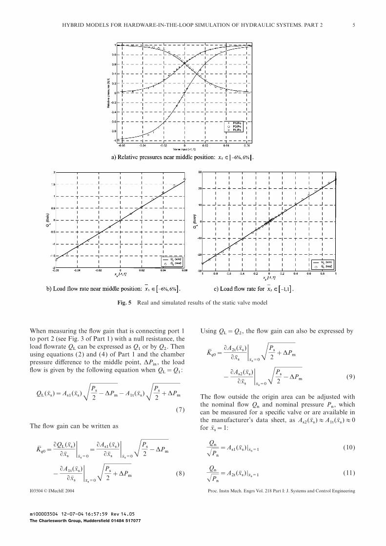
Fig. 5 Real and simulated results of the static valve model

When measuring the flow gain that is connecting port 1 Using QL=Q2 , the flow gain can also be expressed byto port 2 (see Fig. 3 of Part 1) with a null resistance, theload flowrate QL can be expressed as Q1 or by Q2 . Then

K9 q0=qA2t(x: s)qx: s Kx:

s=0SPs

2+DPmusing equations (2) and (4) of Part 1 and the chamber

pressure difference to the middle point, DPin , the loadflow is given by the following equation when QL=Q1 : −

qAs2(x: s)qx: s Kx:

s=0SPs

2−DPm (9)

QL(x: s)=As1(x: s)SPs2−DPm−A1t(x: s)SPs

2+DPm The flow outside the origin area can be adjusted with

the nominal flow Qn and nominal pressure Pn , which(7) can be measured for a specific valve or are available in

the manufacturer’s data sheet, as As2(x: s)#A1t(x: s)#0The flow gain can be written as for x: s=1:

Qn√Pn

=As1(x: s) |x:s=1

(10)K9 q0=qQL(x: s)qx: s Kx:

s=0=qAs1(x: s)qx: s Kx:

s=0SPs

2−DPm

Qn√Pn

=A2t(x: s) |x:s=1

(11)−qA1t(x: s)qx: s Kx:

s=0SPs

2+DPm (8)


mi00003504 12-07-04 16:57:59 Rev 14.05



The leakage flow can be expressed as a function of and its occurring frequency (natural frequency of thethe relative valve chamber pressures, P9 1=P1 /Ps and system) with the results of the simulation of a linearP9 2=P2 /Ps , using equations (2) and (3) of Part 1 when version of the whole system. The experimental blockQ1=Q2=0: diagram used to measure the natural frequency is shown

in Fig. 6. The system has to run in closed loop around Xp0qlk(x: s)=qs1+qs2 because of the different cylinder areas and because of thedifficulties in setting the valve middle position. The system=As1(x: s)

√Ps(1−P9 1)+As2(x: s)√Ps(1−P9 s) is linearized around [P10 P20 Xp0 Vp0 X9 s0 ]T. These

(12) values are obtained from the steady state conditions ofvelocity and acceleration equal to zero, which occur forqlk(x: s)=q1t+q2t X9 s0=0.009 where P1=P10 and P2=P20. In this situation

=A1t(x: s)√PsP9 1+A2t(x: s)

√PsP9 2 (13) the resulting force is zero, i.e. A1P10+Mg−A2P20=0and, with Ps=P10+P20 [9], the equilibrium pressuresAssuming the conditions P9 1#1 and P9 2#0, and usingare given byequations (12) and (13), new relations can be stated for

the leakage flow and leakage flow derivative at a certainspool position. If the leakage flow curve is available, a P10=

A2Ps−Mg

A1+A2, P20=

A1Ps+Mg

A1+A2(18)

measurement at a certain position (x: s>0) can be used;otherwise the leakage at x: s=1 can be set to a very small

where g is the acceleration due to gravity.value or even zero:At the position Xp0=82 mm the chamber volumes are

qlk|P91=1P92=0

=√PsAs2(x: s) (14) almost the same. The cylinder areas are A1=1.2566×10−3 m2 and A2=8.7650×10−4 m2.

The valve static characteristics at the linearized pointsqlk|P91=1P92=0

=√PsA1t(x: s) (15) have the measured values

qqlkqxs KP91=1P92=0

=√PsqAs2(x: s)qx: s KP91=1

P92=0

(16) kq1=qQ1qx: s KX9

s0

=4.76×10−4S Ps2Pn

m3 /s;

qqlkqxs KP91=1P92=0

=√PsqA1t(x: s)qx: s KP91=1

P92=0

(17) kq2=qQ2qx: s KX9

s0

=4.76×10−4S Ps2Pn

m3 /s

Using equation (3) for the pseudo-section functions, tenequations can be stated to solve for the k

iand k

it pseudo- kp1=qP1qx: s KX9

s0

=19Ps Pa, kp2=qP2qx: s KX9

s0

=−15.6Ps Pasection parameters model. Thus, using equations (4),(5), (8), (9), (10), (11), (14), (15), (16) and (17), andconsidering that the leakage flows and their derivatives where k

q1is the flow gain at X9 s0 , k

q2 is the flow gainare zero for x: s=1 (where P9 1=1 and P9 2=0), the pseudo- at X9 s0 , k

p1 is the pressure gain (in chamber 1 at X9 s0 ,section equation parameters k

i, [see equation (3)], are and k

p2 is the pressure gain in chamber 2 at X9 s0 . Theas following: flow–pressure coefficients are then defined as

k1=−2.136, k2=1.602×10−2, k3=4.561

kc2=−kq2

kp2

, kc1=kq1

kp1

(19)k4=−8.084×10−2, k5=1.563×10−2

k1t=−2.145, k2t=7.276×10−3, k3t=4.602

k4t=−4.208×10−2, k5t=1.092×10−2

The results for the relative pressures and load flowratesobtained from the simulation of the static valve modelare presented in Fig. 5.

3.2 Cylinder model

3.2.1 The effective bulk modulus

The effective bulk modulus be, was estimated through theFig. 6 Block diagram to measure the natural frequencycomparison of the maximum cylinder piston acceleration


mi00003504 12-07-04 16:57:59 Rev 14.05



The linearized cylinder and valve equations are expressedin state space format and were simulated in the SimulinkA[10] environment:

C dp1dp2dvpdxpD=tNNNNNNNNv

−be1V1

Kc1 0 −be1V1

A1 0

0 −be2V2

Kc2be2V2

A2 0

A1M

−A2M

−f

M0

0 0 1 0

uNNNNNNNNw

Fig. 7 Acceleration versus frequency plot

×Cdp1dp2dvpdxpD+tNNNNNNNv

be1V1

Kq1

0

−be2V2

Kq2

0

0 1

0 0

uNNNNNNNw

Cdx: sg D

CdvpdxpD=C0 0 1 0

0 0 0 1DCdp1dp2dvpdxpD(20) Fig. 8 Effective bulk modulus versus chamber pressure

where V1=V01+A1Xp0 and V2=V02+A2(L−Xp0) arethe equilibrium volumes and where V01=3×10−5 m3 have the values B=9.71×10−10 and C=1.15×10−3 :and V02=5×10−5 m3 are used for dead volumes of thelines and valve chambers respectively. M represents all

be=105+P

BP+C(21)

the mass in motion and equals 80 kg. The linearizedversion of the friction model (Part 1) [7] is only valid

where B (Pa−1) and C are constants related to the oilfor small displacements ( less than 15 mm) where the sealcharacteristics of the model proposed in reference [11].deformation (variable z) is equal to the piston displace-

ment xp ; i.e. it is assumed that the piston is in the stiction3.2.2 The cylinder leakage conductancestate. The friction factor f is then intended to model all

the friction effects (valve and cylinder) that occur when The internal cylinder leakage is assumed laminar and isthe spool velocity sign have fast changes. represented by a conductance defined as

The effective bulk modulus be and friction factor f wereestimated by an optimization process that minimizes the glkc=

qlkcP1−P2

(22)distance (in the acceleration–frequency plane) betweenthe real and simulated piston maximum acceleration. The The leakage flowrate is measured indirectly in the follow-amplitudes of the acceleration signals measured with ing way. In the initial piston position xp=0, port 2 ofbe1=7.7×108 Pa, be2=9.6×108 Pa and f=8100 N s/m the valve was trapped, port 1 is open to atmosphere andare presented in Fig. 7. The piston acceleration was the cylinder was allowed to run in a free way with ameasured with a high bandwidth accelerometer from 1 to heavy load. The piston position and chamber pressure130 Hz. The experience shown in Fig. 6 was repeated for were measured over a long period Dt of time in orderseveral source pressures in order to evaluate the effective to obtain a constant velocity in steady state, vps . Thebulk modulus as a function of the pressure. Figure 8 shows leakage conductance can then be calculated fromthe evolution of the real be with the chamber pressureand be calculated with equation (21). The parameters glkc=

vpsA2P2

(23)for the equation (21) were obtained by optimization and


mi00003504 12-07-04 16:57:59 Rev 14.05



The piston position and the pressure in chamber 2 were positive velocities. The new estimated parameters are thenmeasured for a period of time Dt=200 s. The total

FCOn=89.26 N, (FSn−FCOn)=160.3 Ndisplacement, in this period, was 1504 mm, and thepressure mean value was P2=5.28 bar. The value

vSn=0.0251 m/s, Kvn=1387 N s/mobtained for the internal leakage conductance was

FCOp=110.2 N, (FSp−FCOp)=150.8 Nglkc=1.248×10−14 m3 /s Pa.

vSp=0.0152 m/s, Kvp=818.4 N s/m3.2.3 Friction model

where the subscripts n and p indicate negative and positiveEstimation of the static parameters FCO, FS, vS and Kv andvelocities respectively.the dynamic parameters s0 and s1 for the LuGre friction

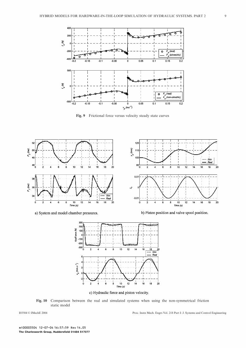
The comparison of the measured static frictionalmodel (see section 3 in Part 1 [7]) are presented below.forces and those obtained from the symmetric and non-symmetric static friction models is presented in Fig. 9.(a) Identification of the static parameters. The static

parameters are estimated from the velocity–frictionalforce curve measured with constant velocities. The sample

(b) Identification of the dynamic parameters. The strategytime was 5 ms, with the frictional forces and velocitiesfor the identification of the dynamic parameters s0 and s1being calculated with 20 samples in order to minimizeconsists in matching the real hydraulic force with thethe noise effects. The experiments at constant velocitiesequivalent hydraulic force, obtained for the same con-were performed with closed-loop velocity control.ditions, from the simulation of the non-linear valveAt constant velocity (a steady state situation, ap=0),plus cylinder model. The non-symmetric static frictionwith the platform in the horizontal position, the frictionparameters were used. The identification used open-force can be measured through the chamber pressuresloop experiments, with the valve and cylinder models[see equation (5) in Part 1]:enhancing the visibility of the dynamic parameters. The

Ff=P1A1−P2A2 (24) system working in the horizontal direction was excitedwith a sinusoidal signal with sufficient amplitude to leadThe frictional force was measured for constant velocitiesthe system in and out of the stiction state; i.e. thebetween −0.2 and 0.2 m/s.resulting force should be, during simulation, larger andAt constant velocity the state variable z of the frictionlower than the breakaway force.model [equations (10) to (12) of Part 1] is constant,

An optimization method, such as that used for esti-dz/dt=0, and the friction force can be estimated frommation of the static parameters, was used to identify the

Ff= [FCO+(FS−FCO) e−(vp/vS)2 ] sgn (vp)+Kvvp (25) dynamic parameters. The cost function is

where FCO , FS , vS and Kv are the estimated staticparameters and Ff is the estimated frictional force. cf (Fh , Fhm , s)= ∑

n

k=1[Fh(k)−Fhm(k, s)]2 (27)

For the parameter estimation the least-squares methodwas used for the cost function cf:

where Fh(k) is the k sample of the real hydraulic force(sample time equal to 10 ms) and Fhm (k, s) is the

cf= ∑n

i=1[Ff(vi)−Ff(vi)]2 (26)

hydraulic force that results from the model simulationwith the same initial conditions, for the same time instant.

where vi

are the measured velocities.The utilization of the hydraulic force as the comparisonThe cost function was calculated for each parameter

force results from the following simplification. The netset (FCO , FS , vS , Kv ) given by the Simplex algorithmacceleration force is given byused in the fminsearch function of the MATLABA [12]

optimization toolbox [13]. Initial values for the para-meters were obtained from the measured velocity versus M

dvpdt=Fh−Ff (28)

frictional force curve. The static parameters to be usedare those that minimize the cost function.

With the mass used in the tests (piston plus rod), as theFor a symmetrical friction model, i.e. the same

maximum values of M dvp /dt are less then 0.05 N, thismodel parameters for positive and negative velocities,

force is negligible when compared with the hydraulic andthe estimated parameters are

frictional forces.FCO=101.8N, FS−FCO=153.0N The comparison of the hydraulic forces, the cylinder

chamber pressures, the spool position and the pistonvS=0.019 m/s, Kv=1090 N s/m

velocity, when simulating the model with the non-symmetrical friction static parameters, is presented inAs the measured frictional forces denote different para-Fig. 10. The estimated dynamic parameters are s0=meters for different signs of velocity, the model can be

enhanced with different parameters for negative and 2.114×107 N/m and s1=2.914×103 N s/m.


mi00003504 12-07-04 16:57:59 Rev 14.05



Fig. 9 Frictional force versus velocity steady state curves

Fig. 10 Comparison between the real and simulated systems when using the non-symmetrical frictionstatic model


mi00003504 12-07-04 16:57:59 Rev 14.05



4 HARDWARE-IN-THE-LOOP SIMULATION the usual spring and damper components (spring stiff-ness equal to 1010 N/m and the damper coefficient equalEXPERIMENTSto 1010 N/m s) and the seal friction model only considersthe viscous friction component. The overall system needsA SimulinkA block implementing the cylinder hybrid

state chart [7] and the valve model was used. The model a third-order fixed-step solver with a 2 ms step size inorder to run properly, negating real-time operation withwas simulated in real time with a third-order explicit

solver and a fixed step size of 0.5 ms. low-cost hardware.Closed-loop position control experiments, with point-

to-point position trajectory as the input reference signal,were performed. Figure 11 shows the comparisons betweenthe two experiments when controlled by proportional 5 CONCLUSIONScontrol, with the proportional constant equal to 50 anda moved mass of 80 kg. A model of a hydraulic system composed of a high-

performance proportional valve and a hydraulic cylinderThe experiment presented in Fig. 12 intends to evaluatethe performance of the real and simulated systems when presented in Part 1 [7], was fully parametrized. Most

of the used models are semiempirical with their para-the desired input trajectories are steps and ramps. In thisexperiment a pressure source with Ps=120 bar was used meters being calculated with simple methods or by

optimization. The static valve parameters are calculatedwith a proportional gain Kp=100.From the results of the above experiments it can be by solving a non-linear equation system. This equation

system is specified in order to reproduce the relevantsaid that the system model presents a satisfactory per-formance at small velocities and at trajectories with static characteristics available from the manufacturer’s

data or from experimental measurements. The parametershigh-frequency content. A similar set of simulations wasproduced using a commercial library of hydraulic com- of the dynamic part of the valve and of the friction model

are determined with optimization techniques.ponents [14]. The cylinder end stops are modelled with

Fig. 11 HILS experimental and simulated results


mi00003504 12-07-04 16:57:59 Rev 14.05



Fig. 12 Experimental and simulation results for input trajectories with high frequency contents

2 Burrows, C. R. Fluid power systems—an academic per-The main goal of this work was to obtain not toospective. JHPS J. Fluid Power Systems, January 1998,complex models allowing their use in HILS experiments.29(1), 26–32.The developed models are reasonably accurate and the

3 Lennevi, J., Palmberg, J. and Jansson, A. Simulation toolwhole system can be simulated in real time with a third-for the evaluation of control concepts for vehicle driveorder explicit solver with a fixed step size of 0.5 ms.systems. In Proceedings of the 4th Scandinavian Inter-Closed-loop position control experiments were performednational Conference on Fluid Power, Tampere, Finland,

with the overall model running in a low-cost real-time September 1995.card from dSPACEA. The results were compared with 4 Maclay, D. Simulation gets into the loop. Instn Electl Engrsthe behaviour of the real system, with the comparison Rev., May 1997, 109–112.being very satisfactory. 5 Otter, M. M., Schlegel, M. and Elmqvist, H. Modelling and

realtime simulation of an automatic gearbox using Modelica.In Proceedings of the European Simulation Symposium

ACKNOWLEDGEMENT (ESS ’97), Passau, Germany, October 1997.6 DS1102 DSP Controller Board, Technical Manuals (dSPACE

This work was funded by FCT under the programme gmbH, Paderborn).POCTI. 7 Ferreira, J. A., Gomes de Almeida, F., Quintas, M. R. and

Estima de Oliveira, J. P. Hybrid models for hardware-in-the-loop simulation of hydraulic systems. Part 1: theory.

REFERENCES Proc. Instn Mech. Engrs, Part I: J. Systems and ControlEngineering, 2004, 218(I0), 000–000.

8 Ferreira, J. A. Modelacao de Sistemas Hidraulicos1 Edge, K. A. The control of fluid power systems—respondingpara Simulacao com hardware-in-the-loop. PhD thesis,to the challenges. Proc. Instn Mech. Engrs, Part I: J. Systems

and Control Engineering, 1997, 211(I2), 91–110. University of Aveiro, Aveiro, Portugal, 2003.


mi00003504 12-07-04 16:57:59 Rev 14.05



9 Gomes de Almeida, F. Model reference adaptive control of 12 MATLAB—The Language of Technical Computing, Tech-a two axes hydraulic manipulator. PhD thesis, University nical Manuals.of Bath, Bath, 1993. 13 Coleman, T., Branch, M. A. and Grace, A. Optimization Tool-

10 Simulink—Dynamic System Simulation for MATLAB, box, 1999 (The Math Works, Inc., Nanch, Massachusetts).Technical Manuals. 14 Beater, P. Hylib—Library of Hydraulic Components for Use

11 Yu, J., Chen, Z. and Lu, Y. The variation of oil effective with Dymola, 2001 (Dynasim AB, Sweden).bulk modulus with pressure in hydraulic systems. Trans.ASME, J. Dynamic Systems, Measmt Control, March 1994,116, 146–149.


mi00003504 12-07-04 16:57:59 Rev 14.05


Hybrid models for hardware-in-the-loop simulation of ...

Documents

Transcript of Hybrid models for hardware-in-the-loop simulation of ...