Hybrid 3D Modeling of Large

Landscapes from Satellite Maps

Project in Lieu of Thesis

for

Master’s Degree

The University of Tennessee, Knoxville

Advisors:

Dr. Mongi Abidi

Dr. Besma Abidi

Vijayaraj Alagarraj

Fall 2003

1

Abstract

Virtual Reality based geographic information systems are successfully employed

today for real-time visualization in such diverse fields as urban planning, city planning

and architectural design. A Virtual Reality based software solution allows the interactive

visualization of high resolution 3D terrain data over an intra and internet. Due to

advanced software technology and innovative data management concepts, large amounts

of data may be processed in real time. Digital elevation models, high resolution satellite

images, 3D buildings and vector data provide real life applications with the information

to display excellent high quality representations of complex terrains and landscapes.

In this project a 3D hybrid model of the Port Arthur Harbor using satellite imagery

and Virtual Reality Modeling Language (VRML) software is built. The 3D textured

terrain model is created by draping satellite images over the Digital Elevation Map

(DEM). To make the scene more realistic, synthetic vegetation at different levels of detail

is added to the model. A bridge model similar to the Martin Luther King Bridge in Port

Arthur, TX, is also added to the terrain model. Harbor buildings, ships, cranes and other

3D synthetic models are placed on the terrain model at different levels of detail. Finally,

after creating a realistic scene of the Port Arthur Harbor, a movie was generated using the

overall 3D model. The movie illustrates the various landscape characteristics and can be

used for further surveillance tasks such as sensor placement scenarios.

2

Table of Contents

Abstract ........................................................................................................... 1 List of Figures................................................................................................. 3 List of Tables .................................................................................................. 6 1. Introduction................................................................................................. 7

1.1 Background........................................................................................................ 8

1.2 Proposed Approach ......................................................................................... 10

2. Image Mosaicing....................................................................................... 12 2.1 Mosaicing of Non Geo-referenced data........................................................... 12

2.2 Mosaicing of Geo-referenced Data ................................................................. 14

3. 3D Digital Terrain Modeling .................................................................... 15 4. Texture Mapping....................................................................................... 17 5. Level of Detail (LOD) Models ................................................................. 23

5.1 Discrete LOD................................................................................................... 23

5.2 Continuous LOD.............................................................................................. 24

5.3 View Dependent LOD ...................................................................................... 24

5.4 Local Simplification Operators ....................................................................... 25

6. Navigation in VRML models ................................................................... 28 6.1 Virtual Reality Model Language...................................................................... 28

6.2 Custom Navigation in VRML........................................................................... 30

7. Experimental Results ................................................................................ 32 7.1 Software Used .................................................................................................. 32

7.2 Image Mosaicing.............................................................................................. 37

7.3 3D Terrain Model Creation............................................................................. 40

7.4 Port Arthur Harbor Simulated Additions ........................................................ 43

7.4.1 Bridge Model Overlay .................................................................................. 43

7.4.2 Harbor Buildings Modeling and Overlay..................................................... 45

7.4.3 Adding a Ship, Crane and Truck .................................................................. 46

7.4.4 Vegetation Modeling and Overlay................................................................ 47

7.5 Level of Detail.................................................................................................. 50

7.6 Camera Modeling, Animation, and VRML Navigation ................................... 53

8. Conclusion ................................................................................................ 56 References:.................................................................................................... 57

3

List of Figures

Figure 1: City model of Zurich rendered with Terrain View [34]……… 4

Figure 2: Example application of 3D-city-models [35]………………… 6

Figure 3: Port Arthur digital images (a) aerial satellite image (DOQQ) (b)

digital elevation map………………………………………… 7

Figure 4: Bridge in the 3D model……………………………………….. 8

Figure 5: Proposed approach flow diagram…………………………… 8

Figure 6: Top row shows the input images and bottom row shows the

output image of the pixel based image mosaicing [55]………. 10

Figure 7: (a) ENVI pixel based image mosaicing window, (b) ENVI geo-

referencing window………………………………………….. 10

Figure 8: Geo-referenced based image mosaicking example (a) input

images, (b) output mosaiced image [56]…………………….. 11

Figure 9: Traditional processing of aerial imagery for the generation of

elevation data [12]……………………………………………. 12

Figure 10: Terrain modeling (a) triangular mesh (b) rectangular mesh.. 13

Figure 11: Texture mapping geometry……………………………………. 17

Figure 12: Computer-generated perspective transformation of downtown San

Jose, CA. Perspective view generated by ESL (now TRW

Sunnyvale, CA). (a) high oblique aerial source image (1 ft

resolution); (b) subsection of the source image with 3D models

overlaid; (c) low oblique wire-frame perspective view of 3D

models; (d) low oblique image perspective transformation output.

© TRW, Inc……………………………………………………. 19

Figure 13: High and low oblique, computer-generated perspective views of

the area around Irish Canyon, CO. Source data courtesy of STX

Corp. Perspective views generated by ESL (now TRW Sunnyvale,

CA).R TRW, Inc……………………………………………….. 20

Figure 14: View-dependent LOD [34]……………………………………. 22

4

Figure 15: Edge collapse and inverse split [34]…………………………… 23

Figure 16: Virtual-edge or vertex-pair collapse [34]……………………… 24

Figure 17: Triangle collapse [34]…………………………………………. 24

Figure 18: Cell collapse. [34]……………………………………………… 25

Figure 19: Vertex removal operation [34]……………………………….. 26

Figure 20: Cosmo player navigation controls [29]………………………. 29

Figure 21: Viewports in 3DS Max. [38]………………………………….. 30

Figure 22: (a) Wire frame mode, (b) Smooth and highlight mode, (c) Edged-

face mode in 3DS Max…………………………………………. 31

Figure 23: Snap shot of TreeMaker software [http://www.TreeMaker.nl]… 32

Figure 24: Snap shot of design workshop Lite software [www.artifice.com] 32

Figure 25: PlantVR software snap shot

[http://www.avic.sc.chula.ac.th/plantvr]………………………….. 33

Figure 26: Tree factory plug-in for 3D Max………………………………… 33

Figure 27: The Panorama factory software input and output images

[www.panoramafactory.com]……………………………………………..…. 35

Figure 28: Pixel based image mosaicking input (4 quads of Port Arthur, TX)

and output image (mosaiced Port Arthur, TX) [55]……………… 36

Figure 29: Geo-referenced mosaic (a) Port Arthur, TX (b) San Diego, CA… 36

Figure 30: Band math input and output images. (a) False color DOQQ and

(b) True color DOQQ…………………………………………… 37

Figure 31: (a) DOQQ and (b) DEM of Port Arthur, TX…………………… 38

Figure 32: Port Arthur 3D model………………………………………….. 38

Figure 33: (a) DOQQ, (b) DEM, (c) Port Arthur 3D textured terrain model 39

Figure 34: (a) San Diego, CA, DOQQ 2.5 meter resolution, (b) San Diego,

CA DEM 30 meter resolution…………………………………… 39

Figure 35: 3D model of San Diego………………………………………… 39

Figure 36: DOQQ color conversation. (a) Monochrome DOQQ, (b) False

color applied after contrast stretching in each band and (c) green

and white color band DOQQ uses green and white to substitute

black and white bands………………………………………….. 40

5

Figure 37: Knoxville input maps (a) One meter DOQQ, (b) 30 meter DEM.. 40

Figure 38: Knoxville 3D model……………………………………………… 41

Figure 39: Terrain model with downloaded bridge (a) Front view and (b)

Side view……………………………………………………….. 41

Figure 40: The real picture of the Martin Luther Kings Bridge in Port Arthur,

Texas……………………………………………………………. 42

Figure 41: (a) Downloaded bridge model [39] (b) altered bridge within 3D

studio max……………………………………………………… 42

Figure 42: (a), (b), (c) & (d) show views of the terrain model with new

embedded bridge model……………………………………….. 42

Figure 43: (a) & (b) Roof texture for the harbor buildings taken from the

satellite image…………………………………………………. 43

Figure 44: (a) & (b) Building front side texture applied from photographs of

the buildings [43]……………………………………………… 43

Figure 45: (a) and (b) Brick textures applied to sidewalls of the building [43] 43

Figure 46: (a) and (b) Harbor buildings with roof and front side textures

applied……………………………………………………………. 43

Figure 47: (a) Harbor buildings before correction, (b) after correction……… 44

Figure 48: (a) 3D ship model [40] (b) 3D truck model [41] (c) 3D crane

model [41]……………………………………………………….. 44

Figure 49: (a), (b) show the terrain model with ship and cranes, (c)shows

additional truck to the Harbor model……………………………. 44

Figure 50: VRML tree models created using TreeMaker………………….. 45

Figure 51: (a) Growth function and (b) leaf shape………………………….. 46

Figure 52: Plant model created using PlantVR Software…………………… 47

Figure 53: (a) & (b) Terrain model with vegetation added…………………. 47

Figure 54: Tree LODs………………………………………………………. 49

Figure 55: Static LOD transition with simple geometry and a tree LOD group 49

Figure 56: Tree LOD group is placed on the Harbor Terrain model………… 50

Figure 57: (a) Video camera model, (b) Video camera placed on the terrain

model and its field of view……………………………………… 50

6

Figure 58: (a) Satellite image zooming window, (b) VRML model of a

selected area in the zooming window…………………………… 51

Figure 59: (a) Harbor model with sphere sensors (red sphere) (b) view from

one of the sphere touch sensor…………………………………… 52

Figure 60: Example of hyper linking with anchor node……………………… 52

Figure 61: (a) & (b) Port Arthur Harbor 3D model with embedded bridge,

ship, buildings, cranes, vegetation models……………………… 53

Figure 62: Video clip layout………………………………………………… 53

List of Tables

Table1: Difference between traditional and image perspective transformation texture

mapping……………….………………………………………………………….18

Table 2: LOD models and their file size………………………………………….51

7

1. Introduction

Many real-time graphics and Virtual Reality (VR) applications aim to immerse the

user in an outdoor scenario composed to a large extent of natural phenomena like plants,

trees, mountains, etc. Some of the most successful virtual reality applications are based

on outdoor settings. Among these applications are flight simulators, tactical training

systems, video games, and urban reconstruction projects. Outdoor environments are

typically flat and sparsely occluded and the area that can be observed by the user is rather

large.

A desired characteristic of the outdoor scene is that the user be able to move freely

over a large area without reaching an artificial border too fast. The environment should

contain significant detail (e.g., leaves on trees) even at close inspection to obtain a

realistic impression. The successful simulation of a large virtual environment represented

with a high degree of fidelity requires construction, run-time management, rendering, and

network transmission of very large geometric databases. Traditionally, research has

focused on the problem of real time rendering of very large geometric databases.

Powerful rendering hardware for polygonal models has been developed for that purpose.

In combination with texture mapping, level of detail (LOD) rendering, and scene culling,

even large scene databases can be rendered in real time as shown in the example of

Figure 1.

Figure 1: City model of Zurich rendered with Terrain View [34]

8

Despite the advances in state of the art graphics technology, the craving for even

more realism often defeats the purpose when the large scene databases become difficult

to handle. We see three areas where improvement is needed:

• Modeling of natural environments: The construction of a large number of

detailed models is extremely labor intensive. While models of artificial

structures such as machines or buildings are relatively easily obtained from

CAD sources, this is not true for plants and other natural phenomena. The use

of texture maps (ex photographs) reduces modeling costs, but this shortcut

becomes painfully obvious when inspecting models in close-up views.

Instancing (i.e. using the same model multiple times) is also easily detected

and destroys the user’s belief in the virtual world.

• Storage requirements: A very large geometric database requires significant

storage. Today’s typical workstations have enough memory to store scene

databases that by far exceed the capacity of the image generator. However, if

only a small portion of an extensive virtual environment is visible at any

time, and the application allows the user to cover large distances, the actual

database can easily exceed memory capacity. Loading data from a disk in real

time has its own set of problems; a compact representation that allows

holding all or a large portion of the scene database is highly preferred.

• Networking: If the geometry database is to be distributed over a network, a

compact representation is even more essential. The rapid growth of Internet-

based VR applications that suffer from notoriously low and unpredictable

bandwidth drives the desire for compact geometric representations that can be

transmitted in a shorter time.

1.1 Background Most publications [3, 4, 7, 9, and 12] discuss building 3D city models by using 3D

CAD and GIS systems. Usually these refer to solutions for single projects that were

produced with very high manual labor expenditure, without taking into account existing

digital maps and plans. Many users already have digital maps in 2D GIS at present,

9

which can be used in building 3D city models if a little additional information is

supplemented.

This data refinement from 2D to 3D presupposes the expansion of the data model

of the existing 2D GIS by the third dimension. In a strict sense this form of modeling

represents 2.5D GIS. The expression 2.5D GIS provides confusion outside the geodetic

field, for example in the fields of architecture, computer animation and Virtual Reality.

For this reason, in the following discussions we call the expansion to the third dimension

3D city models.

The provided 3D city models can be delivered to different users for further

processing as well as visualization and animation (see Figure 2). The refinement of

previous 2D databases represents an efficient and economic solution for building 3D city

models.

Figure 2: Example application of 3D-city-models [35]

A major distinction needs to be made between indoor and outdoor scenes. Indoors, a

scene is constructed from a set of interconnected rooms. In outdoor scenes there are

landscapes of plains, hills and valleys upon which buildings, roads, fields, and lakes can

be placed.

10

1.2 Proposed Approach The main task of this project is to create a realistic model of the Port Arthur Harbor

in Texas and generate a simulated movie showing all the details in that 3D model. This

can be achieved by the following steps. First, gather information about the area to be

modeled (Port Arthur, Texas, in this case). The 3D model can be created in a number of

ways; one is by using various digital satellite images such as Digital Ortho Quadrangle

Quads (DOQQ), Digital Elevation Maps (DEM) and Digital Terrain Models (DTM) [55].

(a) (b)

Figure 3: Port Arthur digital images; (a) aerial satellite image (DOQQ), (b) digital

elevation map

The aerial satellite image shown in Figure 3(a) can be draped on the digital

elevation map to create the terrain's textured 3D model of the area of interest. But the

terrain 3D model depends on the resolution of the image and maps used. For example if

high resolution aerial images are used more texture information in the terrain model will

be available. By using high resolution digital elevation maps better registered 3D models

are obtained. Once the first step of the collection of the aerial satellite images & digital

elevation maps of the area of interest is finished, the next step is to create a terrain model

by draping the aerial image on the DEM. Digital elevation maps do not account for the

elevation of bridges, buildings, and other objects that appear in aerial images because

11

they are created at ground level in the 3D model. Due to this fact, the bridge in the 3D

model collapsed (see Figure 4) and looks unrealistic and therefore needs to be altered. To

correct for this, the texture of the bridge is removed and replaced by a synthetic 3D

bridge model.

Figure 4: Bridge in the 3D model

The third step is to address the addition of vegetation to the terrain model. Different

species of trees, small plants, and grass can be placed at different levels of detail. This

makes the scene more colorful and realistic. For harbor modeling, a few additional

objects are required such as ships, cranes, harbor buildings, trucks, and other machinery.

By adding these models and placing at appropriate locations the scene will look more

realistic.

Figure 5: Proposed Approach Flow Diagram

Collection and mosaicking of satellite aerial images

Overlay satellite image over Digital Elevation Map

Create Port Arthur, TX harbor terrain model

Create synthetic bridge similar to Martin Luther Kings Bridge in Port Arthur, TX

Fuse the synthetic bridge with the Port Arthur terrain model

Create harbor building 3D models with texture taken from the satellite aerial images.

Fuse the building model with the terrain model

Add ship, boat, vegetation around the bridge, crane 3D models to the terrain model

Create virtual movie with the realistic 3D model of Port Arthur Harbor

12

The remainder of this report documents details of the project. Chapter 2 presents the

theory of image mosaicing and various methods used. An overview of the digital terrain

modeling is given in Chapter 3. Chapter 4 documents the theory that supports texture

mapping. Chapter 5 addresses different types of level of detail and local simplification

operators for mesh simplification. To handle easy navigation and viewing 3D models

through intra or internet issues, Chapter 6 presents navigation in VRML models. The

results from this integration are given in Chapter 7.

2. Image Mosaicing

The following sub_section discusses various theoretical issues of image mosaicing.

Image mosaicing is the process of registering or mosaicing two or more images to form a

single large image. There are two different kinds of image mosaicing: pixel based

methods and geo-referenced methods.

2.1 Mosaicing of Non Geo-referenced Data Two or more images with or without overlap can be mosaiced together using a

pixel based method. The first image is considered as the reference image and the

following images as secondary images. In the case of images with an area of overlap the

pixel values of the secondary image are matched and registered to the reference image. If

there is no overlap between the two images then a base image is created and the two

images placed together on that base to form the final single image.

This method is preferable for non geo-referenced images. A number of

commercial software packages are available for image mosaicing using pixel based

methods. Any number of images can be put together to create a longer image from the

entire input series of images. In the result section, Figure 28 shows the output image

mosaiced using a pixel based method. The image sequence used has a minimum of 20%

overlap. The output image will be best when the image sequence has more than 50%

overlap. Figure 6 illustrates the pixel based method using input images with a minimum

of 20% overlap. The output image shows red vertical lines corresponding to the edges

between input images.

13

Figure 6: Top row shows the input images and bottom row shows the output image of the

pixel based image mosaicing [55]

Image mosaicing tools are available in ENVI software. Images with or without

overlap can be mosaiced using this software. ENVI is special purpose software designed

to process aerial, airborne and satellite images. It works in the IDL (Interactive Data

Language) environment and is powerful software for environment visualization. With

this software we can import many images (with or without overlap) to create a mosaic.

The image mosaicing window in ENVI software is shown in Figure 7.

(a) (b)

Figure 7: (a) ENVI pixel based image mosaicing window, (b) ENVI geo-referencing

window

14

2.2 Mosaicing of Geo-referenced Data A geo-referenced image is an image in which their coordinates in real world units

reference the pixels. The real world units can be latitude and longitude. Geo-referenced

mosaicing is used to overlay multiple geo-referenced images by finding pixels in multiple

images with the same latitude and longitude values.

The geo-referenced data consists of individual images and the accompanying

geodetic information (in most cases X, Y coordinates of the NW and SE corner of the

image are enough) or orthoimages. Orthoimages are created based on the digital terrain

modeling (DTM) and the corresponding original image. The coordinates of a point

projected on the original image are computed using co-linear equations based on the

ground coordinates. Height is interpolated from the DTM. It is recommended to use

software which can export geo-referenced files (IRAS/C, HMR Descartes, ArcINFO or

RV32, etc...) and input formats: GEOTIFF (.tiff), TIFF World (.tfw). The output format

usually matches the input format. Figure 8 below shows the mosaicing of geo-referenced

images.

(a) (b)

Figure 8: Geo-referenced based image mosaicking example (a) input images, (b) output

mosaiced image [56]

Notice the differences in brightness between the orthoimages in Figure 8 (a) due to

different weather conditions (cloudiness, fog, air humidity, etc.). During recording in real

situations ortho rectification is never ideal, so in overlapping areas, a mismatch between

orthoimages called the "ghost effect" can take place. Advanced mosaicing software has

the ability to remove these effects. Some areas (area with too much diversity) still need

15

manual correction. After the image mosaicing, a large variation in the quads is still seen.

This is due to high data volume. Further processing such as edge feathering, color

normalization and tonal correction can be done to get more accurate and less distorted

images.

3. 3D Digital Terrain Modeling

The collection of remote digital terrain models, by sensed data has traditionally been

based on stereo conjugate triangulation producing single stereo models. These models

have typically been obtained from aerial photography and, more recently, stereo overlap

in satellite-borne push broom sensors. The shift from analog input (film) to digital

imagery has added some degree of automation in DEM collection through the application

of various correlation techniques. However, even with these more advanced techniques,

processing has remained model-centric.

The processing of satellite data is essentially the same with the use of strips or

overlapping frame images. The general steps are outlined in Figure 9:

Figure 9: Traditional processing of aerial imagery for the generation of elevation data[12]

Pre-evaluation of the visual impact of large construction projects (such as electric

power plants) in the surveillance of large landscapes (examples: harbor, airport) has

lately received a great deal of attention. Two methods have commonly been used to

create synthetic terrain models; one is to paint the proposed area or object onto a

landscape photograph and the other is to build a three dimensional scaled model.

16

The first method lacks objectivity as it depends on an artist's skill, and the number of

views generated is restricted because each view must be separately painted. Using a

model case, the view point can be animated, but construction of the model is very time

consuming and expensive; camera angles may be restricted due to space limitations, and

the resulting images are very artificial looking.

In order to overcome these disadvantages, Uno et al. [15] developed a graphic

system which overlays computer generated images onto a background photograph,

Peibush et M. [4] proposed an anti-aliasing method for montages using digital filtering,

and Porter et al. [13] presented a method which creates composite complex 3D images

using an "a-channel" (8 bit). In [9], the authors proposed a montage method, in which a

computer generated image of the proposed construction is overlaid onto a background

photograph with fog and shadow effects. However, with this method the viewpoint is

restricted to the available background photos and cannot be animated.

A number of methods for generating 3D terrain models from contour lines have been

described. They can be separated into two classes [12]: (1) filling the area between

contour lines with a triangular mesh [1, 2], or (2) filling it with a rectangular mesh [5, 7,

8]. In both cases, the main aim has been to generate views for flight simulators; i.e., to

display mountains at some distance from a considerable height. Because the viewpoint is

at a high altitude, the range of distances from the viewpoint to various points on the

landscape is not very large. Therefore, patches of constant size, independent of distance

from the viewpoint, are generally satisfactory. A bird's eye animation of the Los Angeles

basin was made in this fashion by the Jet Propulsion Laboratory (JPL) [6].

Figure 10: Terrain modeling, (a) triangular mesh. (b) rectangular mesh

17

However, in environmental assessment images the viewpoint will usually be very

near the ground, i.e., at the level of the human eye. In this case, a small patch size results

in very inefficient processing for regions distant from the viewpoint, while a large patch

size results in inadequate image quality in regions near the viewpoint.

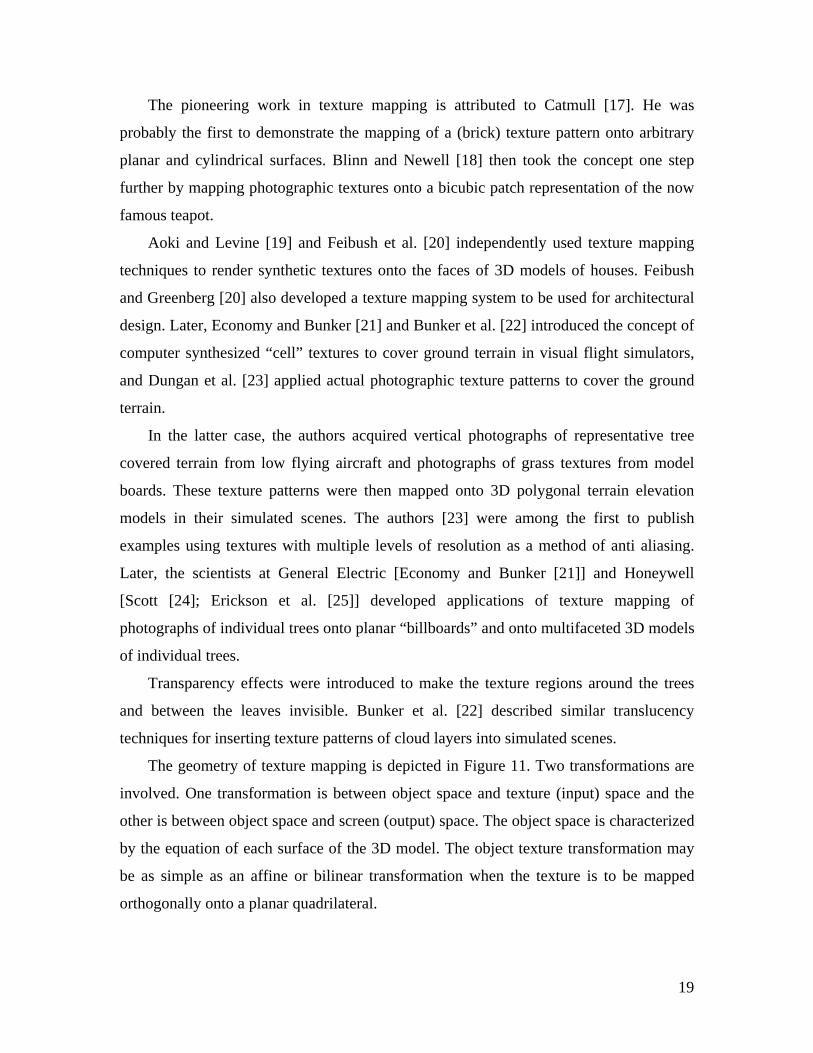
4. Texture Mapping

In the last few years texture mapping has become a popular tool in the computer

graphics industry. Texture mapping provides an easy way to achieve a high degree of

realism in computer generated imagery with little effort. Over the last decade, texture

mapping techniques have advanced to the point where it is possible to generate real time

perspective simulations of real world areas by texture mapping every object surface with

texture from photographic images of these real world areas.The techniques for generating

such perspective transformations are variations in traditional texture mapping that in

some circles have become known as the Image Perspective Transformation or IPT

technology.

Some of the salient challenges that must be met to achieve these images and movies

and to create effective visual simulations include:

(1) How to create high resolution models from heterogeneous input sources such as

magazine pictures, direct photography, digital imagery, artist’s renderings, and the like.

(2) How to align or register the imagery with the geometry models and smoothly

blend different models from different sources so that nothing stands out unnaturally.

(3) How to deal efficiently with very large databases to keep rendering times down

while maintaining realism, knowing that:

• Geometry models may include both natural terrain and urban features, where

the former may contain millions of (regularly or irregularly spaced) elevation

values.

• Many large, oblique, high resolution images may be needed to cover the vast

expanse of natural terrain.

(4) How to correct source imagery distortions so that resulting output views are

faithful to reality, considering:

18

• Source images are often oblique views.

• Source images are formed by various camera and sensor types often with

nonstandard geometries.

(5) How to pre-warp the output images so they project naturally onto domes, pancake

windows, and the like.

(6) How to perform these myriad tasks fast enough for real time or high speed non

real time display [18].

Although the distinction between the IPT texture mapping variation and traditional

texture mapping may be subtle, these differences are worth noting. Some of the important

differences between the image perspective transformation and the traditional texture

mapping technique are summarized in the following and listed in Table 1.

Table1. Difference between Traditional and Image Perspective Transformation

Texture mapping [18]

Traditional Texture Mapping Image Perspective Transformation

• Texture maps are frequently synthetic.

• Relatively few small texture maps are

used.

• Texture maps are frequently repeated on

multiple objects or faces.

• Texture maps are typically face-on views.

• Textures are often arbitrarily mapped onto

objects without concern for distortions.

• Alignment of texture maps with the object

faces is generally performed manually.

• 3D object models are typically built

independently from the texture maps.

• Polygon object models and rendering

approaches are typically used.

• Texture maps are actual photographs or

remote sensing images of real world areas.

• Many large images are used as texture

maps.

• Textures are unique per object face.

• Texture maps are typically oblique views.

• Photogrammetry techniques are often used

to project the textures onto object faces to

correct for camera acquisition geometry.

• Photogrammetry and remote sensing

techniques are frequently used to

automatically align the textures with the

object faces.

• Photogrammetry techniques are frequently

used to build 3D object models of terrain

and urban structures from the imagery.

• Height field, voxel and polygon object

models and rendering approaches are all

used.

19

The pioneering work in texture mapping is attributed to Catmull [17]. He was

probably the first to demonstrate the mapping of a (brick) texture pattern onto arbitrary

planar and cylindrical surfaces. Blinn and Newell [18] then took the concept one step

further by mapping photographic textures onto a bicubic patch representation of the now

famous teapot.

Aoki and Levine [19] and Feibush et al. [20] independently used texture mapping

techniques to render synthetic textures onto the faces of 3D models of houses. Feibush

and Greenberg [20] also developed a texture mapping system to be used for architectural

design. Later, Economy and Bunker [21] and Bunker et al. [22] introduced the concept of

computer synthesized “cell” textures to cover ground terrain in visual flight simulators,

and Dungan et al. [23] applied actual photographic texture patterns to cover the ground

terrain.

In the latter case, the authors acquired vertical photographs of representative tree

covered terrain from low flying aircraft and photographs of grass textures from model

boards. These texture patterns were then mapped onto 3D polygonal terrain elevation

models in their simulated scenes. The authors [23] were among the first to publish

examples using textures with multiple levels of resolution as a method of anti aliasing.

Later, the scientists at General Electric [Economy and Bunker [21]] and Honeywell

[Scott [24]; Erickson et al. [25]] developed applications of texture mapping of

photographs of individual trees onto planar “billboards” and onto multifaceted 3D models

of individual trees.

Transparency effects were introduced to make the texture regions around the trees

and between the leaves invisible. Bunker et al. [22] described similar translucency

techniques for inserting texture patterns of cloud layers into simulated scenes.

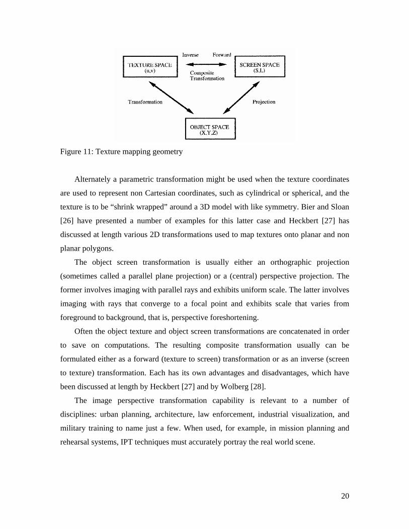
The geometry of texture mapping is depicted in Figure 11. Two transformations are

involved. One transformation is between object space and texture (input) space and the

other is between object space and screen (output) space. The object space is characterized

by the equation of each surface of the 3D model. The object texture transformation may

be as simple as an affine or bilinear transformation when the texture is to be mapped

orthogonally onto a planar quadrilateral.

20

Figure 11: Texture mapping geometry

Alternately a parametric transformation might be used when the texture coordinates

are used to represent non Cartesian coordinates, such as cylindrical or spherical, and the

texture is to be “shrink wrapped” around a 3D model with like symmetry. Bier and Sloan

[26] have presented a number of examples for this latter case and Heckbert [27] has

discussed at length various 2D transformations used to map textures onto planar and non

planar polygons.

The object screen transformation is usually either an orthographic projection

(sometimes called a parallel plane projection) or a (central) perspective projection. The

former involves imaging with parallel rays and exhibits uniform scale. The latter involves

imaging with rays that converge to a focal point and exhibits scale that varies from

foreground to background, that is, perspective foreshortening.

Often the object texture and object screen transformations are concatenated in order

to save on computations. The resulting composite transformation usually can be

formulated either as a forward (texture to screen) transformation or as an inverse (screen

to texture) transformation. Each has its own advantages and disadvantages, which have

been discussed at length by Heckbert [27] and by Wolberg [28].

The image perspective transformation capability is relevant to a number of

disciplines: urban planning, architecture, law enforcement, industrial visualization, and

military training to name just a few. When used, for example, in mission planning and

rehearsal systems, IPT techniques must accurately portray the real world scene.

21

Several non-real time, workstation based systems have made advances in these areas.

These include systems developed by TRW/ESL, General Dynamics Electronics Corp.,

SRI, and the University of California at Berkeley.

TRW’s system renders output scenes by computing texture coordinates for every

screen pixel using an incremental scan line method to evaluate the fractional linear

perspective transformation. This transformation is able to account for the oblique

geometry of the source texture images as well as the viewing perspective associated with

the output. Articles by Devich and Weinhaus [29] and Weinhaus and Devich [30] showed

how to derive the fractional linear transformation coefficients for a planar polygon

independent of the number of its vertices without the need to store u, v (or w) texture

coordinates for each polygon. The only information needed is the camera parameter

model for the texture image and the equation of the plane for the polygon. In fact, the

four coefficients defining the plane need not be carried with the polygon, since they can

be generated from the world coordinates of the vertices.

In this system, none of the imagery, either for the texture of the ground covering or

the sides of urban features, has to be rectified or mosaicked. A simple tiled pyramid is

created for each source image and the appropriate tile (or tiles) is automatically selected

to cover each surface at an appropriate resolution for anti-aliasing. A deferred texturing,

depth buffer technique is used and various re-sampling techniques may be selected to

trade quality for speed, including super sampling and/or EWA on a pyramid.

The EWA technique [31] is a very good method for anti-aliasing, since it samples the

input data within an elliptical “footprint” region that represents the projection of a given

(circular) output pixel. The size and orientation of the ellipse adapts to the geometry and

depends upon the orientation and location of both the input and output cameras and the

orientation of the 3D model surface upon which it is projected. The terrain elevation data,

which originate from a regular grid of elevation values, are automatically reformatted

into a multi resolution triangular surface mesh for each output frame.

This process allows coarser triangles to be used in the background of output images

and finer ones to be used in the foreground. However, before rendering any frame,

surfaces from two levels are blended. This prevents sudden transitions in level of detail

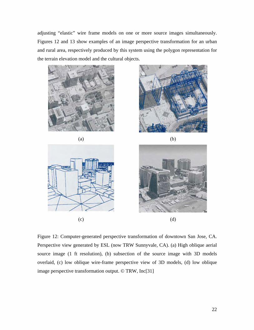
from being observed in motion sequences. Urban features are modeled by interactively

22

adjusting “elastic” wire frame models on one or more source images simultaneously.

Figures 12 and 13 show examples of an image perspective transformation for an urban

and rural area, respectively produced by this system using the polygon representation for

the terrain elevation model and the cultural objects.

(a) (b)

(c) (d)

Figure 12: Computer-generated perspective transformation of downtown San Jose, CA.

Perspective view generated by ESL (now TRW Sunnyvale, CA). (a) High oblique aerial

source image (1 ft resolution), (b) subsection of the source image with 3D models

overlaid, (c) low oblique wire-frame perspective view of 3D models, (d) low oblique

image perspective transformation output. © TRW, Inc[31]

23

(a) (b)

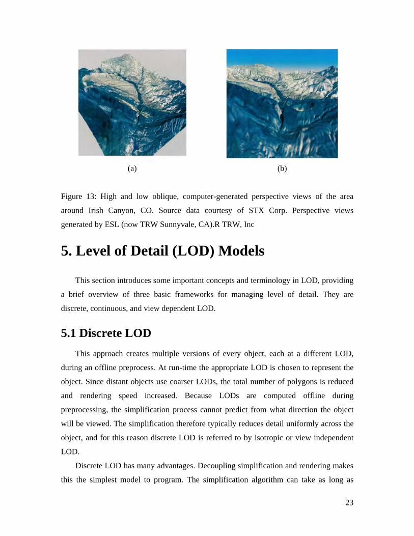
Figure 13: High and low oblique, computer-generated perspective views of the area

around Irish Canyon, CO. Source data courtesy of STX Corp. Perspective views

generated by ESL (now TRW Sunnyvale, CA).R TRW, Inc

5. Level of Detail (LOD) Models

This section introduces some important concepts and terminology in LOD, providing

a brief overview of three basic frameworks for managing level of detail. They are

discrete, continuous, and view dependent LOD.

5.1 Discrete LOD This approach creates multiple versions of every object, each at a different LOD,

during an offline preprocess. At run-time the appropriate LOD is chosen to represent the

object. Since distant objects use coarser LODs, the total number of polygons is reduced

and rendering speed increased. Because LODs are computed offline during

preprocessing, the simplification process cannot predict from what direction the object

will be viewed. The simplification therefore typically reduces detail uniformly across the

object, and for this reason discrete LOD is referred to by isotropic or view independent

LOD.

Discrete LOD has many advantages. Decoupling simplification and rendering makes

this the simplest model to program. The simplification algorithm can take as long as

24

necessary to generate LODs and the run time rendering algorithm simply needs to choose

which LOD to render for each object. Furthermore, modern graphics hardware lends

itself to the multiple model versions created by static LOD, because individual LODs can

be complied during preprocessing to an optimal rendering format. For example,

depending on the particular hardware targeted, developers may convert models to use

features such as triangle strips, display lists, and vertex arrays. These will usually render

much faster than simply rendering the LODs as a unordered list of polygons.

5.2 Continuous LOD Continuous LOD departs from the traditional discrete approach. Rather than creating

individual LODs during a preprocessing stage, the simplification system creates a data

structure encoding a continuous spectrum of detail. The desired level of detail is then

extracted from this structure at run time. A major advantage of this approach is better

granularity since the level of detail for each object is specified exactly rather than

selected from a few pre-created polygons for rendering other objects, which in turn use

only as many polygons as needed for the desired level of detail, freeing up more polygons

for other objects, and so on. Better granularity thus leads to better use of resources and

higher overall fidelity for a given polygon count.

Continuous LOD also supports streaming of polygonal models, in which a simple

base model is followed by a stream of refinement to be integrated dynamically. When

large models must be loaded from disk or over a network, continuous LOD provides

progressive rendering and interruptible loading often very useful properties.

5.3 View Dependent LOD View Dependent LOD extends continuous LOD, using View Dependent

simplification criteria to dynamically select the most appropriate level of detail for the

current view. Thus View Dependent LOD is anisotropic; a single object can span

multiple levels of simplification. For instance, nearby portions of the object may be

shown at higher resolution than distant portions, or silhouette regions of the object shown

at higher resolution than interior regions. This leads to still better granularity: polygons

are allocated where they are most needed within objects as well as among the objects.

25

This in turn leads to better fidelity for a given polygon count, optimizing the distribution

of this scarce resource. Figure 14 shows the view dependent level of detail model.

Figure 14. View-Dependent LOD [34]

Very complex models representing physically large objects, such as terrains, often

cannot be adequately simplified without view dependent techniques. Creating discrete

LODs does not help. The view point is typically quite close to part of the terrain and

distant from other parts, so a high level of detail will provide good fidelity at

unacceptable frame rates, while a low level of detail will provide a good frame rate but

terrible fidelity. Another source of difficult models is scientific visualization, which tends

to produce extremely large data sets that are rarely organized into conveniently sized

objects. Again, View Dependent LOD can enable interactive rendering without manual

intervention or extra processing for segmentation.

5.4 Local Simplification Operators There are various low level local operators that have been used for simplification of

meshes. Each of these operators reduces the complexity of a mesh by some small amount.

5.4.1 Edge Collapse

This operator collapses an edge (Va, Vb) to a single vertex Vnew. This causes the

removal of the edge (Va, Vb) as well as the triangle spanning that edge. The inverse

operator of an edge collapse is a vertex split, which adds the edge (Va, Vb) and the

triangle adjacent to it. Thus, the edge collapse operator simplifies a mesh and the vertex

26

split operator adds detail to the mesh. Figure 15 illustrates the edge collapse operator and

its inverse, the vertex split.

Figure 15. Edge collapse and inverse split [34]

The edge collapse operator has been widely used in view independent simplification,

view dependent simplification, progressive compression, as well as progressive

transmission. There are 2 invariants of the edge collapse operator: half edge collapse and

full edge collapse.

5.4.2 Vertex Pair Collapse

A vertex pair collapse operator collapses 2 unconnected vertices Va and Vb. Since

these vertices do not share an edge, no triangles are removed by a vertex-pair collapse,

but the triangle surrounding Va and Vb are updated as if an imaginary edge connecting Va

and Vb underwent an edge collapse as seen in Figure 16. For this reason, the vertex-pair

collapse operator has also been referred to as a virtual edge collapse. Collapsing

unconnected vertices enables connection of unconnected components as well as closing

of holes and tunnels.

Figure 16. Virtual-edge or vertex-pair collapse [34]

In general, for a mesh with n vertices there can be potentially n^2 virtual edges, so an

algorithm that considers all possible virtual edges will run slowly. Most of the topology

27

simplification algorithms rely on virtual edge collapse; therefore use heuristic choice of

virtual edges only between nearby vertices, considering virtual edge collapse from each

vertex Va to all vertices within a small distance from Va.

5.4.3 Triangle Collapse

A triangle collapse operator simplifies a mesh by collapsing a triangle to a single

vertex Vnew. The edges that define the neighborhood of Vnew are the union of edges of the

vertices Va, Vb, and Vc. The vertex Vnew to which the triangle collapses can be either one

of Va, Vb, and Vc or a newly computed vertex. This is shown in figure 17. A triangle

collapse is equivalent to two edge collapses.

Figure 17 Triangle collapse [34]

A triangle collapse based hierarchy is shallower than an equivalent edge collapse

based hierarchy and thus requires less memory. However, triangle collapse hierarchies

are also less adaptable, since the triangle collapse is a less fine-grained operation than an

edge collapse.

5.4.4 Cell Collapse

The cell collapse operator simplifies the input mesh by collapsing all the vertices in a

certain volume, or cell, to a single vertex. The cell undergoing collapse could belong to a

grid or a spatial subdivision such as an octree or could simply be defined as a volume in

space. The single vertex to which the cell collapses could be chosen from one of the

collapsed vertices or newly computed as some form of average of the collapsed vertices.

Consider a triangular mesh object as shown in Figure 18(a). The vertices of the mesh

are placed in a grid. All the vertices that fall in the same grid cell are then unified into a

single vertex. The vertices are identified in Figure 18(b). All triangles of the original

mesh that have two or three of their vertices in a single cell are either simplified to single

28

edge or a single vertex. This is shown in Figure 18(c). The final mesh is shown in Figure

18(d).

(a) (b) (c) (d)

Figure 18. Cell collapse [34]

5.4.5 Vertex Removal

The vertex removal operator removes a vertex, along with its adjacent edges and

triangles, and triangulates the resulting hole. Triangulation of the hole in the mesh

resulting from removal of vertex v can be accomplished in several ways and one of these

triangulations is the same as a half edge collapse involving vertex v. In this respect

atleast, the vertex removal operator may be considered to be a generalization of the half

edge collapse operator. Figure 19 illustrates the vertex removal operation.

Figure 19 Vertex Removal Operation [34]

6. Navigation in VRML models

6.1 Virtual Reality Model Language VRML is an acronym stands for Virtual Reality Modeling Language and was

designed to create a more friendly and interesting environment for the World Wide

29

Web. VRML incorporates 3D shapes, colors, textures, and sounds to produce both

models of individual objects and virtual worlds that a user could walk and fly through.

VRML uses a platform independent file format for sharing 3D worlds. VRML

worlds can be interactive and animated, and can include embedded hyperlinks to other

Web documents.

If you are a beginner, the ten most important things you need to know about VRML

are:

• VRML files usually have the extension '.wrl'

• They are usually viewed by means of a browser plug-in

• Browser plug-ins can be downloaded free of charge

• Files can be read by any computer platform (Apple Mac, PC, UNIX, Linux, etc.)

• Each file describes a 3D-model (i.e. an object or a world)

• Objects are described by their geometry and appearance (e.g. color, texture map)

• Objects can have behaviors and links added to them

• Models can have lighting, but there are usually no shadows

• There are libraries of existing VRML models that you can download and use

• There are editors to help you build VRML models

VRML has evolved in two phases. VRML 1.0 was adopted in the spring of 1995 and

provided the basic file format, but the worlds were static. The VRML community

immediately began work on strategies for incorporating animated behaviors into VRML.

The current specification, VRML 2.0, supports JAVA, sound, animation, and JavaScript

which allows the world to be dynamic and interactive.

Moving through a 3D space is similar to moving a camera around the scene being

viewed. A VRML viewer is best compared to a video camera that captures and converts

the images onto a screen. The camera has a position and orientation and user movements

in the model are continually repositioning and re-orienting it.

In addition to continuous camera movement, VRML models usually provide a

number of viewpoints: predefined camera locations describing a position and orientation

for viewing the scene. Viewpoints are usually placed at particularly interesting or well

positioned places from which the user may want to see the model. Since only one

30

viewpoint may be active at a time, viewpoints should be seen as a particularly convenient

starting point from which the 3D model can be best explored.

However, as we are dealing with 3D spaces, there are different types of movement

throughout the model. These types of movement are often called navigation modes,

usually simulating walking, flying or rotating.

While most of the browsers have similar layouts of the large model display area and

a control console at the bottom of the window, the exact names and configurations of

navigation modes vary from browser to browser,

6.2 Custom Navigation in VRML VRML97 browsers support a NavigationInfo node. This node specifies a number of

navigation characteristics that determines much of how the user interacts with the world

through the browser.

There may be more than one NavigationInfo node in the scene graph. The node in

effect is the one currently at the top of the NavigationInfo node stack. When a world first

starts, the first NavigationalInfo node is at the top of the stack. As the world evolves,

other NavigationalInfo nodes may be bound to the top location. The currently bound

NavigationalInfo node supplies all of the navigation parameters. If an individual field is

not specified, the default value is used.

The fields of NavigationalInfo are avatarSize, headlight, speed, type, and visibility

Limit. The avatarSize field specifies the size of the user in the world for collision

detection and terrain following. 'Headlight' turns on or off a directional light that tracks

the user's orientation. Speed is the rate of travel through the world. The type field

specifies the mode of navigation. Visibility Limit determines the furthest geometry that is

visible. The remainder of this discussion will focus on the type field.

The type field can be specified with multiple values. Legal values are at least:

"ANY", "WALK", "EXAMINE", "FLY", and "NONE". Browsers may define other

values. Any combination of values may be specified. The allowed navigation type is the

union of all specified values. Specifying "NONE" with other values does not decrease the

range of options.

31

The difference between "WALK" and "FLY" is gravity. In "WALK" mode, the

user's position falls until it collides with some geometry. This allows the user to traverse

across uneven terrain. The user moves in the XZ plane with Y being controlled by

geometry. In "FLY" mode, the y axis value is controlled by the user through various

browser controls.

"EXAMINE" mode allows the user to spin or rotate an object or the world as a

whole. It is not intended as a means for traversing a world. "ANY" allows any navigation

mode that the browser supports. "NONE" disallows all browser based navigation modes.

If your world specifies a NavigationInfo type of "NONE" you must provide a means

to move around the world. This can be done through a variety of means. For example,

Viewpoints Touch Sensors, or Anchors can animate the user's position throughout the

world. If you intend to give the user complete freedom of movement through your world,

you will need to provide an alternate means of user controls. The following paragraph

discusses one such solution.

This mechanism of navigation can be very useful. The world can limit the camera

position and orientation prior to causing a change in the displayed world (see Figure 20).

Figure 20: Cosmo Player Navigation Controls [29]

In this particular world, there is not much to gain by going to a custom navigation

system. There are cases when you need to move in a direction other than the current

camera orientation. For example, you need to fly level through a world where you wish to

look down. Normal browser navigation will cause your flight elevation to drop (you fly

32

where you look). Using custom navigation, you can separate the "looking down" portion

from the "moving around" navigation.

7. Experimental Results

7.1 Software Used 7.1.1 3D Studio Max

3D Studio Max is used for placing synthetic 3D models on the textured terrain

model. With 3D Studio Max, it is easy to create 3D places and characters, objects and

subjects of any type and arrange them in settings and environments to build the scenes for

creating 3D model. It is also easy to animate the characters, set them in motion, make

them speak, sing and dance, or kick and fight and then shoot movies of the whole virtual

scene. In 3DS Max objects are created in viewports. This software also imports geometry

created elsewhere. The object’s parameters can be controlled in the command-panel

rollouts. The objects can be surfaces or splines, 2D or 3D geometry, all positioned in 3D

space.

Lights and Cameras: Light objects are added to create shadows and illumination.

Cameras can be created to shoot movies of your scene.

Materials and Effects: The surfaces of the geometry are further enhanced with

materials, which are created and edited in the Material Editor and mapped to objects in

the scene. Special effects such as particle systems, combustion, atmosphere, and fog can

be added as well.

Keyframe Animation: The objects can then be moved, rotated, or scaled over

multiple time frames to create the animation.

Camera Animation: Cameras can fly through virtual spaces. Virtual camera motion

can be made to match the camera movement taken from video. Motion blur can be added

to camera animation.

Rendering: Once the animation is complete, the finished movie sequence can be

created through rendering. The output of the animation can be a movie file format or a

sequence of still images.

33

The Viewports: When you start 3DS Max, you are presented with a default user

interface. This consists of four viewports surrounded by tools and controls. (See Figure

21)

Figure 21: Viewports in 3DS Max [38]

A view port can display the scene from the front or back, left or right, top or bottom

views. It can also display different angled views such as perspective, user, spotlight, or

camera. Viewports can display geometry in a wire frame mode or several different

shaded modes (see Figure 22). Edged face mode lets you see your selected faces and

shading at the same time.

(a) (b) (c)

Figure 22: (a) Wire frame mode, (b) smooth and highlight mode, (c) edged-face mode in

3DS Max

34

7.1.2 Tree Animation Software

There are many commercial software packages available for tree animation.

Following is a survey on tree animation software and features.

TreeMaker

TreeMaker is a program for generating virtual 3D solid trees. The trees can be saved

in a 3D file format and loaded in a 3D modeling, landscape generator or rendering

program. Different kinds of vegetation models were created using this software and those

models were placed on the Port Arthur textured terrain model. A snap shot of the

software front end is shown in the Figure 23.

Figure 23: Snap shot of TreeMaker Software [57]

Design Workshop Lite

DesignWorkshop(R) Lite is a fast and creative tool for creating spatial models,

images, and walkthroughs, from initial sketches to polished presentations.

With DesignWorkshop, 3D designers can quickly and easily sketch out spatial ideas

in three dimensions, then develop them quickly and easily using flexible CAD-accurate

editing, alignment, and snapping functions. Automatic texture-mapping and real-time

QuickDraw 3D rendering with lights and textures bring design visions quickly to life.

The unique DesignWorkshop modeling environment is based on a live 3D crosshair,

so you can model in real perspective space, using natural click-and-drag style editing to

create, resize, and reshape walls, roofs, openings, etc. The software front end is shown in

the Figure 24.

35

Figure 24: Snap shot of Design Workshop Lite software [58]

PlantVR

PlantVR software is based on L-system. Smooth animation of plant growth can be

done using this software. There are many parameters which can be adjusted and allow the

creation of plant models. Figure 25 shows a snap shot of the PlantVR software

Figure 25: PlantVR software snap shot [59]

Tree Factory Plug-in for 3D Max

Tree Factory is a complete forestry creation toolkit in one robust package. One can

use Tree Factory to generate a wide variety of trees and ground foliage to add realism to

3D Studio MAX and 3D Studio VIZ scenes. Figure 26 shows images and screen shots of

the 3DS Max plug-in.

36

Figure 26: Tree Factory plug-in for 3D Max

7.1.3 ENVI

ENVI (Environment for Visualizing Images) is a revolutionary image processing

system. ENVI was used to create a terrain models by draping satellite aerial images on

digital elevation maps. From its inception, ENVI was designed to address the numerous

and specific needs of those who regularly use satellite and aircraft remote sensing data.

ENVI provides comprehensive data visualization and analysis for images of any size and

any type—all from within an innovative and user-friendly environment. One of ENVI's

strengths lies in its unique approach to image processing—it combines file-based and

band-based techniques with interactive functions. When a data input file is opened, its

bands are stored in a list, where they can be accessed by all system functions. If multiple

files are opened, bands of disparate data types can be processed as a group. ENVI

displays these bands in 8 or 24 bit display windows.

ENVI's display window groups consist of a main image window, a zoom window,

and a scroll window, all of which are re-sizeable. ENVI provides its users with many

unique interactive analysis capabilities, accessed from within these windows. ENVI's

multiple dynamic overlay capabilities allow easy comparison of images in multiple

displays. Real-time extraction and linked spatial/spectral profiling from multi-band and

hyper spectral data give users new ways of looking at high-dimensional data. ENVI also

provides interactive tools to view and analyze vectors and GIS attributes. Standard

capabilities such as contrast stretching and 2-dimensional scatter plots are just a few of

the interactive functions available to ENVI users.

37

ENVI is written in IDL (Interactive Data Language), a powerful structured

programming language that offers integrated image processing. IDL is required to run

ENVI and the flexibility of ENVI is due largely to IDL's capabilities. ENVI provides a

multitude of interactive functions, including X, Y, Z profiling, image transects, linear and

non-linear histogram and contrast stretching, color tables, density slicing, classification

color mapping, quick filter preview, and Region of Interest definition and processing.

7.1.4 The Panorama Factory

This package creates high-quality panoramas from a set of overlapping digital

images. The Panorama Factory transforms the images so that they can be joined

seamlessly into panoramas in which the fields of view can range up to 360 degrees.

Figure 27 shows input images and output image of the panorama factory software.

Figure 27: The Panorama Factory software input(top) and output(bottom) images

The Panorama Factory creates images that rival those made by rotational and

swing-lens panoramic cameras. Not only can The Panorama Factory facilitate creation of

immersive VR worlds, it also provides features for the fine-art panoramic photographer

who wishes to work from ordinary 35 mm images or images captured with a digital

camera.

The Port Arthur satellite aerial images were mosaiced using Panorama factory

software.

7.2 Image Mosaicing The different types of image mosaicing were discussed in Section 2. The results of

the various methods applied to the Port Arthur data are as follows.

38

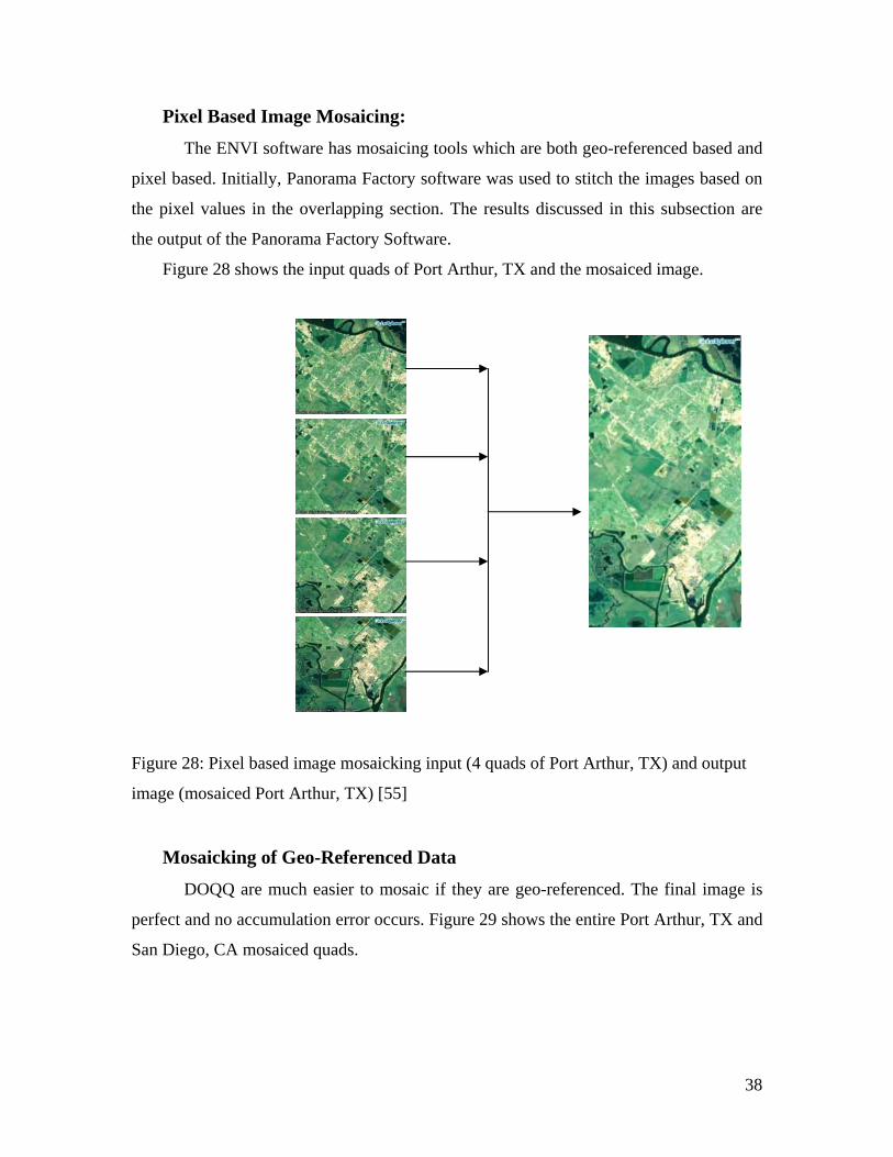
Pixel Based Image Mosaicing:

The ENVI software has mosaicing tools which are both geo-referenced based and

pixel based. Initially, Panorama Factory software was used to stitch the images based on

the pixel values in the overlapping section. The results discussed in this subsection are

the output of the Panorama Factory Software.

Figure 28 shows the input quads of Port Arthur, TX and the mosaiced image.

Figure 28: Pixel based image mosaicking input (4 quads of Port Arthur, TX) and output

image (mosaiced Port Arthur, TX) [55]

Mosaicking of Geo-Referenced Data

DOQQ are much easier to mosaic if they are geo-referenced. The final image is

perfect and no accumulation error occurs. Figure 29 shows the entire Port Arthur, TX and

San Diego, CA mosaiced quads.

39

(a) (b)

Figure 29: Geo-referenced mosaics; (a) Port Arthur, TX, (b) San Diego, CA

Initially all the 1 meter digital orthophoto quadrangles quads downloaded were in

false color format Color Infrared (CIR) band. Using the band math function in ENVI

false color quads were converted to true color. The expression to convert false color

(CIR) to true color is

• New Red Channel 0.9*B2 + 0.1*B1

• New Green Channel 0.7*B3 + 0.3*B1

• New Blue Channel B3

Where B1, B2 & B3 are false colors in the R, G, and B channels

Figure 30 (a) shows false color DOQQ converted to true color in Figure 30 (b) by

using the expression above.

Figure 30: Band math input and output images. (a) False color DOQQ and (b) true color

DOQQ

40

16 quads were used for Port Arthur, TX and 14 quads were used for San Diego, CA.

All 30 false color quads were converted into true color DOQQ and then used for image

mosaicing.

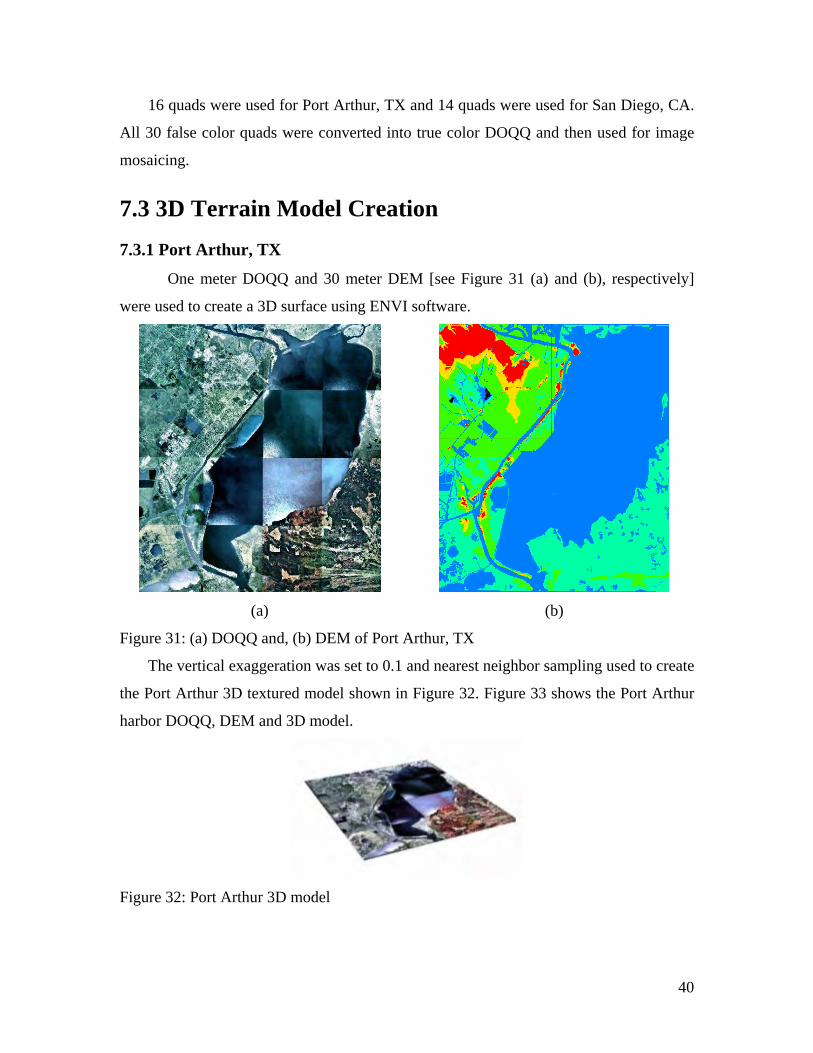
7.3 3D Terrain Model Creation 7.3.1 Port Arthur, TX

One meter DOQQ and 30 meter DEM [see Figure 31 (a) and (b), respectively]

were used to create a 3D surface using ENVI software.

(a) (b)

Figure 31: (a) DOQQ and, (b) DEM of Port Arthur, TX

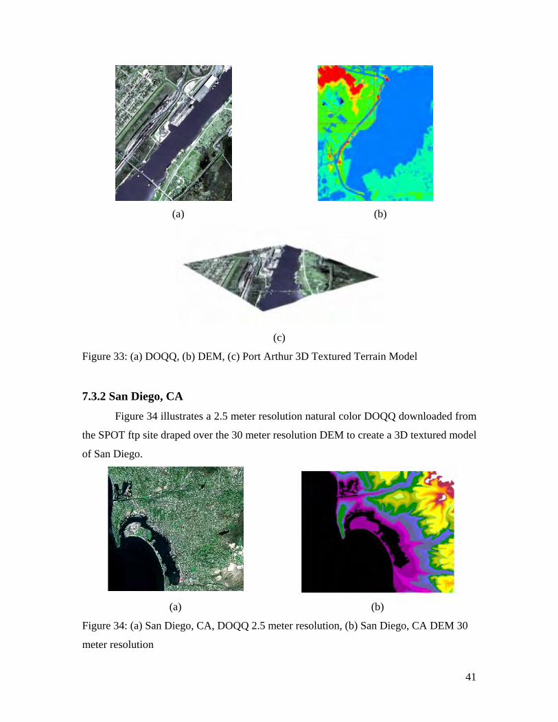
The vertical exaggeration was set to 0.1 and nearest neighbor sampling used to create

the Port Arthur 3D textured model shown in Figure 32. Figure 33 shows the Port Arthur

harbor DOQQ, DEM and 3D model.

Figure 32: Port Arthur 3D model

41

(a) (b)

(c)

Figure 33: (a) DOQQ, (b) DEM, (c) Port Arthur 3D Textured Terrain Model

7.3.2 San Diego, CA Figure 34 illustrates a 2.5 meter resolution natural color DOQQ downloaded from

the SPOT ftp site draped over the 30 meter resolution DEM to create a 3D textured model

of San Diego.

(a) (b)

Figure 34: (a) San Diego, CA, DOQQ 2.5 meter resolution, (b) San Diego, CA DEM 30

meter resolution

42

The vertical exaggeration and other parameters are set to the same values as before.

The output 3D Model of San Diego is shown in Figure 35.

Figure 35: 3D Model of San Diego

7.3.3 Knoxville, TN

The DOQQ available for Knoxville, TN is a one meter black and white, geo-

referenced image. First, false coloring is applied to the black and white DOQQ as seen in

Figure 36.

(a) (b) (c)

Figure 36: DOQQ color conversation. (a) Monochrome DOQQ, (b) false color applied

after contrast stretching in each band and, (c) green and white color band DOQQ uses

green and white as substitute for black and white bands

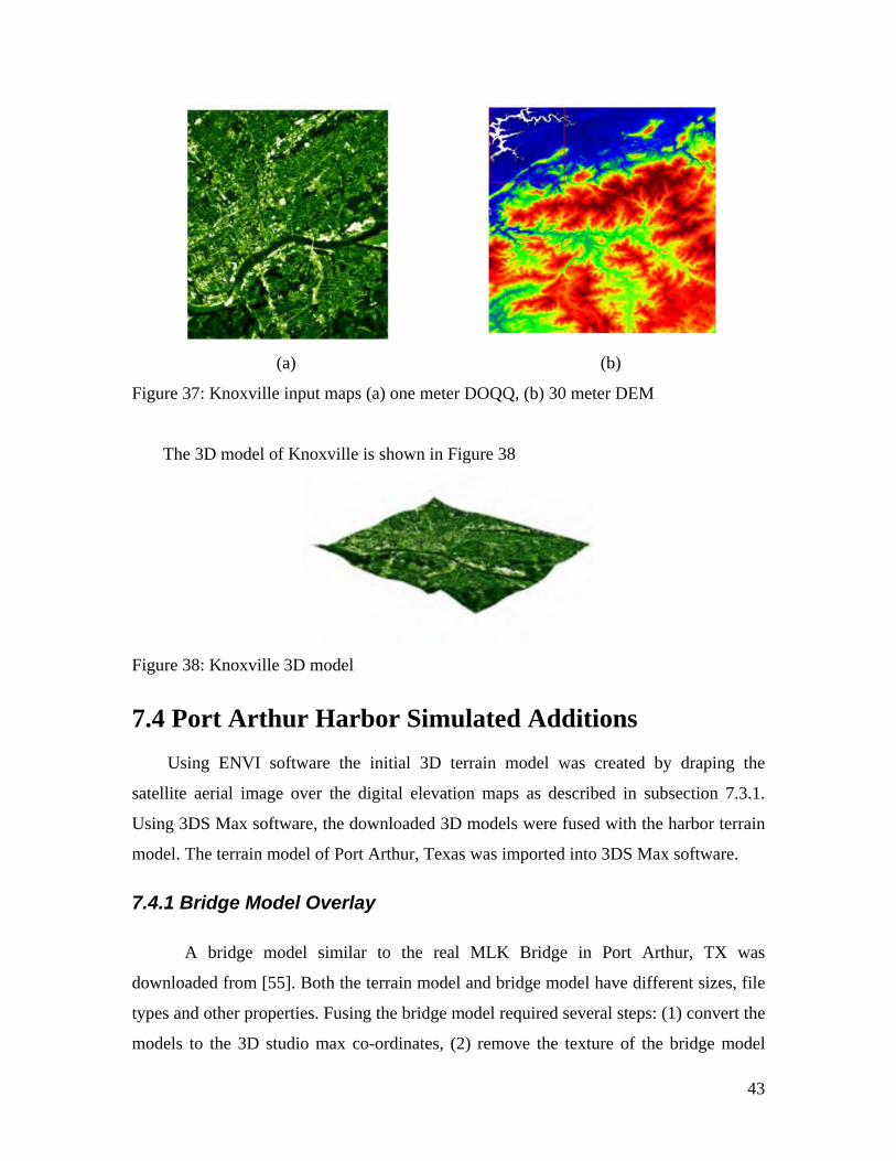
The green and white color band DOQQ and 30 m DEM were used to create the 3D

textured model of Knoxville as shown in Figure 37.

43

(a) (b)

Figure 37: Knoxville input maps (a) one meter DOQQ, (b) 30 meter DEM

The 3D model of Knoxville is shown in Figure 38

Figure 38: Knoxville 3D model

7.4 Port Arthur Harbor Simulated Additions Using ENVI software the initial 3D terrain model was created by draping the

satellite aerial image over the digital elevation maps as described in subsection 7.3.1.

Using 3DS Max software, the downloaded 3D models were fused with the harbor terrain

model. The terrain model of Port Arthur, Texas was imported into 3DS Max software.

7.4.1 Bridge Model Overlay

A bridge model similar to the real MLK Bridge in Port Arthur, TX was

downloaded from [55]. Both the terrain model and bridge model have different sizes, file

types and other properties. Fusing the bridge model required several steps: (1) convert the

models to the 3D studio max co-ordinates, (2) remove the texture of the bridge model

44

from the aerial image and (3) merge the imported bridge model onto the terrain model.

The output 3D hybrid model is shown in the Figure 39.

(a) (b)

Figure 39: Terrain model with downloaded bridge. (a) Front view and, (b) side view

After merging the bridge model, it still looks a bit different from the real Martin

Luther King Bridge in Port Arthur Harbor, Texas. The bridge was then modified and

reconstructed to look more like the real bridge in Port Arthur [Figure 40]. This was done

using 3DS Max software.

Figure 40: Martin Luther King Bridge in Port Arthur, TX

Figure 41 shows the downloaded bridge model and the modified bridge model.

(a) (b)

Figure 41: (a) Downloaded bridge model [39], (b) bridge altered within 3D studio

max

In figure 42 several views of the terrain model with the new bridge model are shown.

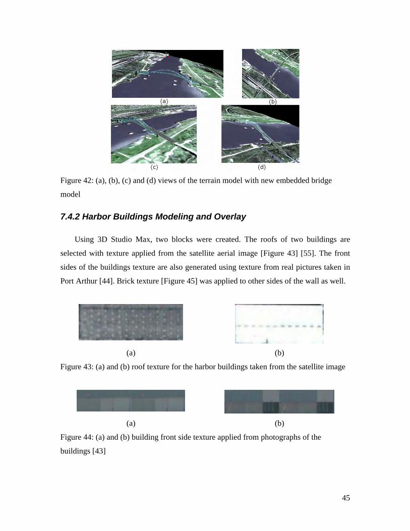
45

Figure 42: (a), (b), (c) and (d) views of the terrain model with new embedded bridge

model

7.4.2 Harbor Buildings Modeling and Overlay

Using 3D Studio Max, two blocks were created. The roofs of two buildings are

selected with texture applied from the satellite aerial image [Figure 43] [55]. The front

sides of the buildings texture are also generated using texture from real pictures taken in

Port Arthur [44]. Brick texture [Figure 45] was applied to other sides of the wall as well.

(a) (b)

Figure 43: (a) and (b) roof texture for the harbor buildings taken from the satellite image

(a) (b)

Figure 44: (a) and (b) building front side texture applied from photographs of the

buildings [43]

46

(a) (b)

Figure 45: (a) and (b), brick textures applied to sidewalls of the building [43]

Figure 46 shows the harbor building with all the above textures applied.

(a) (b)

Figure 46: (a) and (b), harbor buildings with roof and front side textures applied

Figure 47 illustrates the terrain model with the additions of the textured buildings.

(a) (b)

Figure 47: (a) Harbor buildings before correction, (b) after correction

7.4.3 Adding a Ship, Crane and Truck

A ship, crane, and truck 3D models (as seen in Figure 48) were also obtained [55]

and added to the Port Arthur harbor terrain model (Figure 49).

(a) (b) (c)

Figure 48: (a) 3D ship model [40], (b) 3D truck model [41], (c) 3D crane model [41]

47

(a) (b) (c)

Figure 49: (a), (b) terrain model with ship and cranes, (c) shows additional truck added to

the harbor model

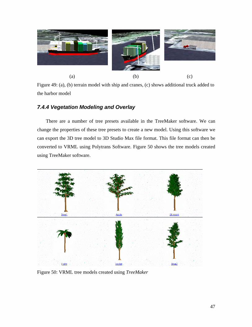
7.4.4 Vegetation Modeling and Overlay

There are a number of tree presets available in the TreeMaker software. We can

change the properties of these tree presets to create a new model. Using this software we

can export the 3D tree model to 3D Studio Max file format. This file format can then be

converted to VRML using Polytrans Software. Figure 50 shows the tree models created

using TreeMaker software.

Figure 50: VRML tree models created using TreeMaker

48

Steps to create a plant in PlantVR software

• Write the initial string

• Set the production rule and end rule

• Compile the initial string and generate the final L-string

• Assign the growth function to each component

• Define the leaf shape, flower shape

• Select the leaf texture to apply

• Set other properties like stem length, node diameter, internodes, time step,

leaf arrangement, etc

• Animate the 3D plant

• Capture each frame and create gif image

The L-system initial string to generate a plant and the generated string after iterations is

shown below.

Initial String prototype

Soybean{

Iterations=6

Angle=45

Diameter=1.5

Axiom=I[-iL][+iL]A

A=I[-P]I[+B]A

P=IIII[\pL][/pL][-pL]

B=IIII[\pL][/pL][+pL]

ENDRULE

B=IL

P=IL

A=IL

}

Generated string = I[-iL][+iL]I[-IIII[\pL]

[/pL][-pL]]I[+IIII[\pL][/pL][+pL]]I[-IIII

[\pL][/pL][-pL]]I[+IIII[\pL][/pL][+pL]]I

[-IIII[\pL][/pL][-pL]]I[+IIII[\pL][/pL]

[+pL]]I[-IIII[\pL][/pL][-pL]]I[+IIII[\pL]

[/pL][+pL]]I[-IIII[\pL][/pL][-pL]]I[+IIII

[\pL][/pL][+pL]]I[-IIII[\pL][/pL][-pL]]

I[+IIII[\pL][/pL][+pL]]IL

49

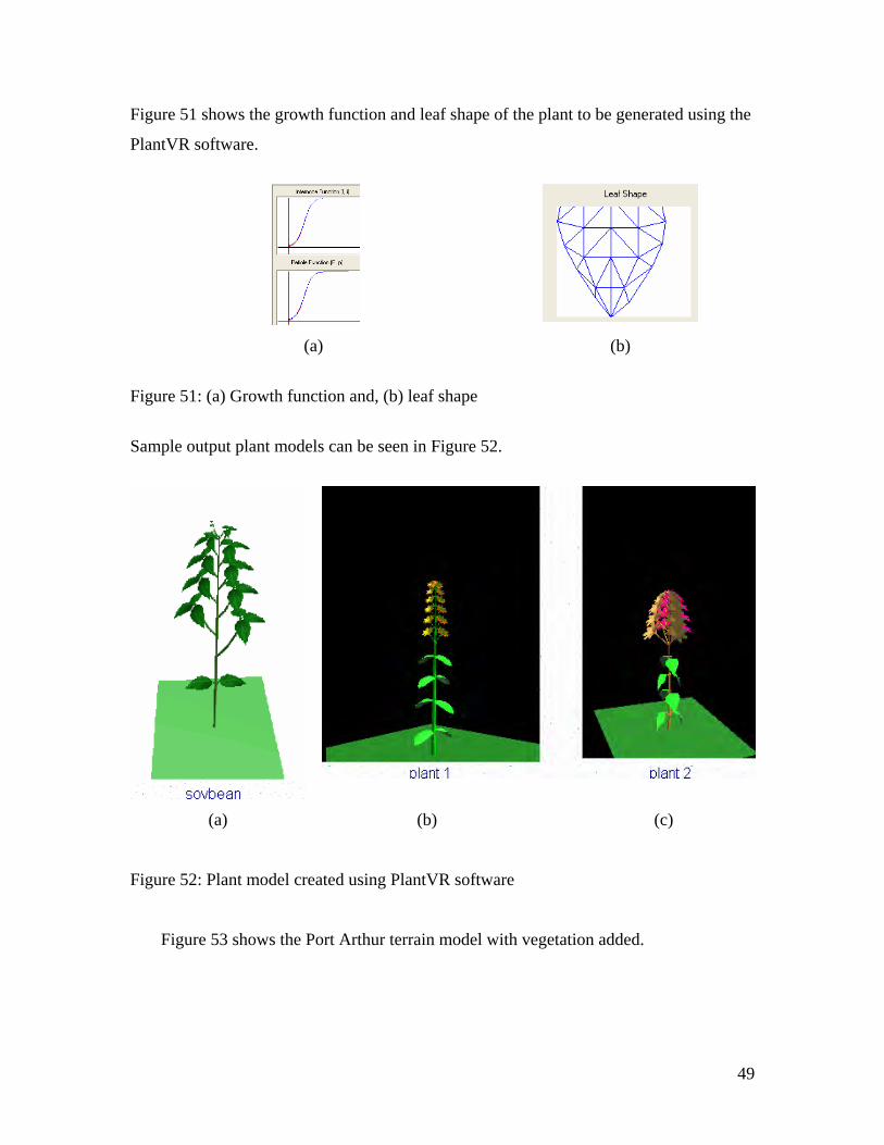
Figure 51 shows the growth function and leaf shape of the plant to be generated using the

PlantVR software.

(a) (b)

Figure 51: (a) Growth function and, (b) leaf shape

Sample output plant models can be seen in Figure 52.

(a) (b) (c)

Figure 52: Plant model created using PlantVR software

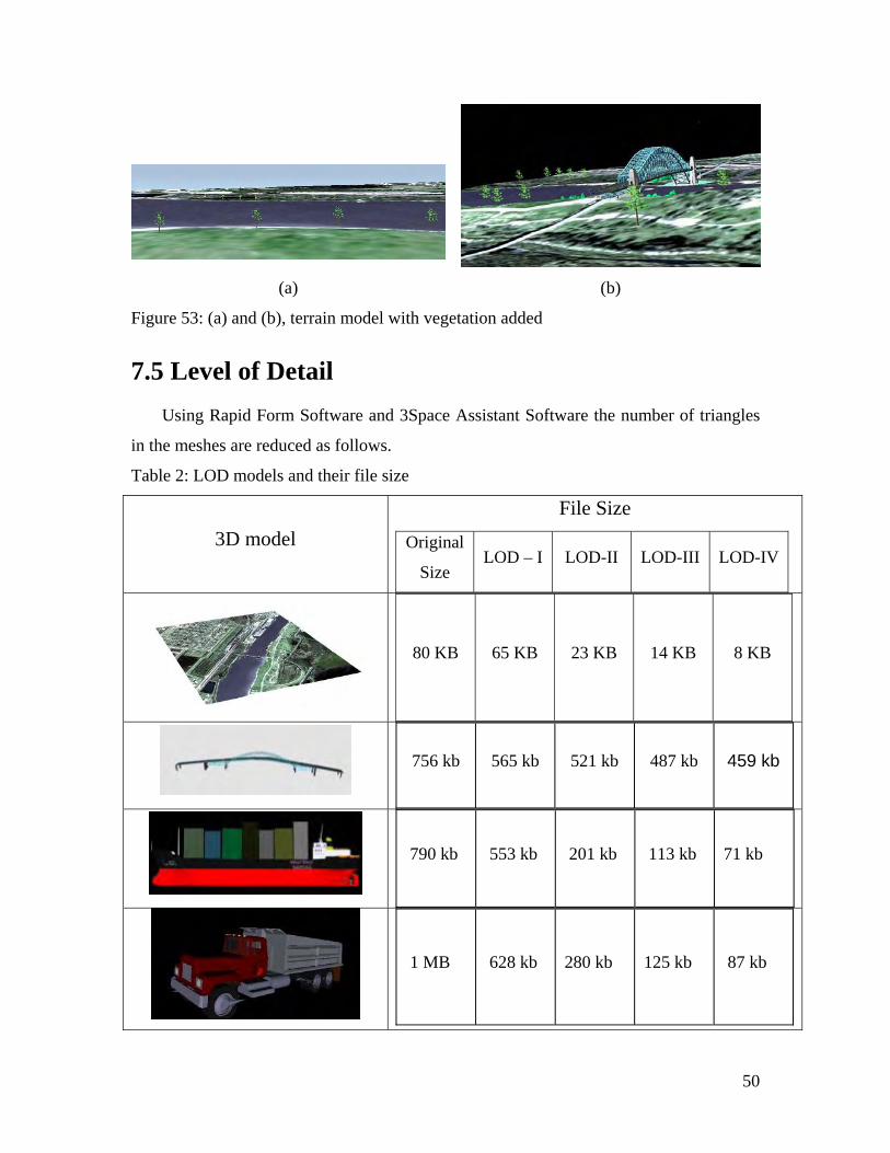
Figure 53 shows the Port Arthur terrain model with vegetation added.

50

(a) (b)

Figure 53: (a) and (b), terrain model with vegetation added

7.5 Level of Detail Using Rapid Form Software and 3Space Assistant Software the number of triangles

in the meshes are reduced as follows.

Table 2: LOD models and their file size

3D model File Size

Original

Size LOD – I LOD-II LOD-III LOD-IV

80 KB 65 KB 23 KB 14 KB 8 KB

756 kb 565 kb 521 kb 487 kb 459 kb

790 kb 553 kb 201 kb 113 kb 71 kb

1 MB 628 kb 280 kb 125 kb 87 kb

51

7.94 MB 6.07 MB 2.54 MB 1.06 MB 614 kb

2.54 MB 1.94 MB 851 kb 395 kb 237 kb

Figure 54 shows Tree LODs created using decimate operations.

Figure 54: Tree LODs

Using the above results, a LOD group was created for each model and placed on the

terrain model. The pre-defined LOD model can be displayed from any particular distance.

Static LODs are only groups of objects placed at particular distances from the viewer at

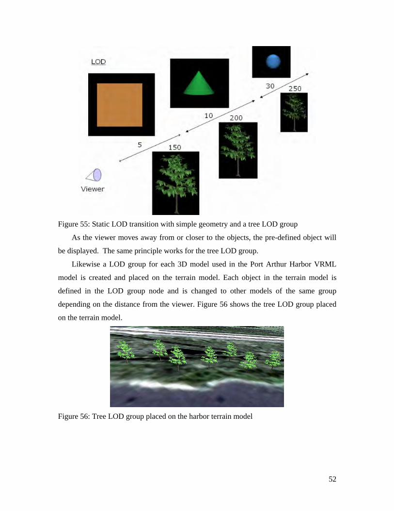
different levels of detail. Figure 55 illustrates the static LOD operations and consists of a

sphere, a cone and a box placed at specific distances from the viewer.

52

Figure 55: Static LOD transition with simple geometry and a tree LOD group

As the viewer moves away from or closer to the objects, the pre-defined object will

be displayed. The same principle works for the tree LOD group.

Likewise a LOD group for each 3D model used in the Port Arthur Harbor VRML

model is created and placed on the terrain model. Each object in the terrain model is

defined in the LOD group node and is changed to other models of the same group

depending on the distance from the viewer. Figure 56 shows the tree LOD group placed

on the terrain model.

Figure 56: Tree LOD group placed on the harbor terrain model

53

7.6 Camera Modeling, Animation, and VRML

Navigation 7.6.1 Video Camera Modeling and Placement

Figure 57 shows the video camera model and its placement on the terrain model.

(a) (b)

Figure 57: (a) Video camera model, (b) video camera placed on the terrain model and its

field of view

7.6.2 Embedding VRML file in html script

To avoid downloading large VRML files for viewing on a personal computer, an

embedding script is written that allows viewing of 3D models through the internet

browser. All the VRML models created earlier are embedded into a html script.

7.6.3 Additional Zooming Function

A zoom feature was also added to help in viewing 3D models of a particular area of

interest. Pre-specified small red boxes denote the areas of interest. By clicking on a red

box a detailed and high resolution map will be displayed. Again, by clicking the detailed

image the 3D model of that part will be displayed in the same window.

Figure 58 shows the satellite zooming window and the embedded 3D model in the

zooming window.

54

Figure 58: (a) Satellite image zooming window, (b) VRML model of a selected area in

the zooming window

Placing the Touch Sensor with Anchor Node for Easy Navigation and Hyper Linking

Create the trigger object (ex: sphere)

Place the anchor in the VRML world

Select an event (ex: hyper linking, jump to another view point)

Link the trigger object with anchor node with predefined event.

An example of the touch sensor with anchor node is shown in the Figure 59.

(a) (b)

Figure 59: (a) Harbor model with sphere sensors (red sphere), (b) view from one of the

sphere touch sensors

55

Upon clicking on the sensor point (green sphere) in Figure 60, which is hyper

linked to another VRML model, the new VRML can be displayed in the same window or

in a different window.

Figure 60: Example of hyper linking with anchor node

7.6.4 Simulated movie from the New Port Arthur Harbor 3D model

Figure 61 shows the final Port Arthur Harbor 3D hybrid model at different views

with each model placed at different levels of detail.

Figure 61: (a) and (b), Port Arthur Harbor 3D model with embedded bridge, ship,

buildings, cranes, vegetation models

3D Studio Max animation uses controllers. The default controllers used are the

position, rotation and scale of the object set with the Move, Rotate and Scale transforms.

56

Other controllers can make the object move and change in different ways. Figure 62

illustrates the video clip layout.

Figure 62: Video Clip Layout

8. Conclusion

The technology to generate arbitrary views of real world areas from photographic

information has evolved from both the computer graphics and flight simulation

industries. Two decades ago representations of real or fictitious scenes were generated

using simple wire frames. Then illumination based shading techniques were developed

that over time have evolved to create increasingly more realistic effects. This was

followed by the introduction of texture mapping a technique that adds realistic looking

synthetic or even photographic texture patterns to faces of objects. Over a decade ago, the

first true perspective transformations of images were published that completely texture

mapped every 3D model in the scene with actual photographic information about the real

world model to which it corresponded.

The popularity of this technology has grown dramatically over the last few years.

Low cost workstation based systems exist today that can present moderate quality 2.5D

transformed views of natural terrain environments in near real time (approximately one

frame per second). This is achieved using modern, general purpose processors and

efficient software, but limited texture information must be specially preprocessed to a

vertical format, mosaiced together, and then stored in memory. Other low cost,

57

workstation based systems are available that can create high quality 2.5D views for

arbitrary mixes of natural terrain and cultural models. They can handle extremely large

amounts of imagery with minimal preprocessing, but they are typically slower, since

these data must be transferred from disk storage. Furthermore, the algorithms must be

general enough to handle urban models as well as the terrain and therefore are not quite

as efficient.

Commercial and military flight simulators as well as some high end workstations can

achieve real time perspective transformation rates for mixed rural and urban areas,

because they use special purpose parallel hardware and make compromises with respect

to algorithms and data loads.

References:

[1] Agui, T., Miyata, K., and Nakajima, M. “A Reconstructing Method of 3D

Mountainous Shapes from Contours”. Trans. IEICE J69-D, 12 (1986), 1905-1912.

[2] Christiansen, N. H. and Sederberg, T. W. “Conversion of Complex Contour Line

Definitions into Polygonal Element Mosaics”. Computer Graphics 12, 3 (1978), 187-192.

[3] Crow, F. C. “Shadow Algorithms for Computer Graphics”. Computer Graphics

1I, 2 (1977), 242-247.

[4] Feibush, E. A., Leroy, M., and Cook, R. L. “Synthetic Texturing Using Digital

Filters”. Computer Graphics 14, 3 (1980), 294-301.

[5] Gardner, G.Y. “Simulation of Natural Scenes Using Textured Quadric Surfaces”.

Computer Graphics 18, 3 (1984), 11-19.

[6] Jet Propulsion Laboratory. “Finale L.A the Movie”. SIGGRAPH '87 Film and

Video Show (1987).

[7] Marshall, R., Wilson, R., and Carlson, W. “Procedure Models for Generating

Three-Dimensional Terrain”. Computer Graphics 14, 3 (1980), 154-162.

[8] Miller, G. S. P. “The Definition and Rendering of Terrain Maps”. Computer

Graphics 20, 4 (1986), 39-48.

58

[9] Nakamae, E., Harada, K., Ishizaki, T., and Nishita, T.A Montage method: “The

Overlaying of the Computer Generated Images onto A Background Photograph”.

.Computer Graphics ~0, 4 (1986), 201-214.

[I0] Nakamae, E., Ishizaki, T., Nishita, T., and Takita, S. “Compositing 3D Images

with Antialiasing and Various Shading Effects”. IEEE Computer Graphics ~

Applications 9, 2 (1989), 21-29.

[11] Nishita, T., Okamura, I., and Nakamae, E. “Shading Models for Point and

Linear Sources”. ACM Transactions on Graphics 4, 2 (1985), 124-146.

[12] Petrie, G. and Kennie, T. J. M. “Terrain Modeling in Surveying and Civil

engineering”. Computer Aided Design i9, 4 (1987), 171-187.

[13] Porter, T. and Duff, T. “Composing Digital Images”. Computer Graphics 18, 3

(1984), 253-259.

[14] Rougelot, 13.. S. “The General Electric Computed Color TV Display.”

Proceedings of the Second University of Illinois Conference on Computer Graphics. In

Pertinent Concepts in Computer Graphics. eds. Faiman, M. andNievergelt, J. University

of Illinois Press (1969), 261-281.

[15] Uno, S. and Matsuka, H. “A General Purpose Graphic System for Computer

Aided Design”. Computer Graphics 13, 2 (1979), 25-232.

[16] Williams, L. “Pyramidal Parametrics”. Computer Graphics 17, 3 (1983), 1-11.

[17] Catmull, E. “Computer Display Of Curved Surfaces”. In Proceedings Of The

Conference On Computer Graphics, Pattern Recognition And Data Structures (Ieee

Computer Society, New York, May 14–16), 1975, 11–17.

[18] Blinn, J. F. And Newell, M. E.. “Texture And Reflection In Computer

Generated Images”. Commun. Acm 19, 10 (May), 1976, 542–547.

[19] Aoki, M. And Levine, M. D. 1978. “Computer Generation Of Realistic Pictures.

Comput. Graph”. 1, 149–161.

[20] Feibush, E. And Greenberg, D. “Texture Rendering System For Architectural

Design. Comput. Aided Des”. 12, 2 (March), 1980, 67–71.

[21] Economy, R. And Bunker, M. “Advanced Video Object Simulation”. In

Proceedings Of The National Aerospace And Electronics Conference (Ieee, New York,

May), 1984, 1065–1071.

59

[22] Bunker, M., Economy, R., And Harvey, J. “Cell Texture—Its Impact On

Computer Image Generation”. In Proceedings Of The Sixth Interservice Industry

Training Equipment Conference, 1984, 149–155.

[23] Dungan, W., Stenger, A., And Sutty, G. “Texture Tile Considerations For Raster

Graphics”. Computer Graphics (Proceedings Of Siggraph), Acm Siggraph 12, 3 (Aug.),

1978, 130–134.

[24] Scott, W. B. “Image System To Unite Computer, Video”. Aviation Week Space

Technol. (May 16), 1983, 70–73.

[25] Erickson, C., Fairchild, K. M., And Marvel, O. “Simulation Gets A New Look”.

Defense Electron. (Aug.), 1984, 76–87.

[26] Bier, E. A. And Sloan, K. R. “Two-Part Texture Mappings”. Ieee Comput.

Graph. Appl. (Sept.), 1986, 40–53.

[27] Heckbert, P. S. “Fundamentals Of Texture Mapping And Image Warping”.

Masters Thesis, Computer Science Division, University Of California, Report No.

Ucb/Csd 89/516., 1989.

[28] Rg, G. “Digital Image Warping”. Ieee Computer Society Press, Los Alamitos,

Ca, 1990.

[29] Devich, R. N. And Weinhaus, F. M. “Image Perspective Transformations”. In

Proceedings Of Spie (Bellingham, Wa, July 29–Aug. 1), 1980, Vol. 238, 322–332.

[30] Weinhaus, F. M. And Devich, R. N.“Photogrammetric Texture Mapping Onto

Planar Polygons”. Graph. Models Image Process, 1997.

[31] Greene, N. And Heckbert, P. “Creating Raster Omnimax Images From Multiple

Perspective Views Using The Elliptical Weighted Average Filter”. Ieee Comput. Graph.

Appl. (June 1986), 21–27.

[32] Li, R., Potential Of High-Resolution Satellite Imagery For National Mapping

Products. Photogrammetric Engineering And Remote Sensing, Vol. 64, No. 12, Pp. 1998,

1165-1170.

[33] Cambray, B. " 3D Modelling in Geographic Database", in: AutoCarto, 11th

International Conference on Computer Assisted Cartography, Minneapolis, 1993

Web Link References

[34] www.Viewtec.ch

60

[35] http://gis1.bv.tum

[36] www.emse.fr

[37] http://home.tiscali.cz

[38] www.3dlinks.com

[39] http://web.nps.navy.mil

[40] http://www.huntfor.com/3d/links.htm

[41] http://cic.nist.gov/vrml/equip.html

[42] www.3dcafe.com

[43] D. Page Port Arthur Digital Images

Tutorial References

VRML Tutorial

[44] www.lighthouse3d.com

[45] www.web3d.com

[46] www.vrmlsite.com

[47] www.3dlinks.com

[48] www.bridgesite.com

[49] http://www.ballreich.net/vrml

[50] http://tom.di.uminho.pt/vrmltut/toc.html

3D Studio Max Tutorial

[51] www.3dcafe.com

[52] www.dform.com

[53] www.tinkering.net

[54] www.3dlinks.com [55] www.mapquest.com

[56] www.inet.hr

[57] http://www.TreeMaker.nl

[58] www.artifice.com

[59] http://www.avic.sc.chula.ac.th/plantvr

61