ORIGINAL ARTICLE

Global ionosphere maps based on GNSS, satellite altimetry, radiooccultation and DORIS

Peng Chen1 • Yibin Yao2,3 • Wanqiang Yao1

Received: 14 July 2015 / Accepted: 7 July 2016

� Springer-Verlag Berlin Heidelberg 2016

Abstract Global ionosphere maps (GIMs) provided by the

global navigation satellite systems (GNSS) data are

essential in ionospheric research as the source of the global

vertical total electron content (VTEC). However, conven-

tional GIMs experience lower accuracy and reliability from

uneven distribution of GNSS tracking stations, especially

in ocean areas with few tracking stations. The orbits of

ocean altimetry satellite cover vast ocean areas and can

directly provide VTEC at nadir with two different wave-

lengths of radio waves. Radio occultation observations and

the beacons of Doppler orbitography and radio positioning

integrated by satellite (DORIS) are evenly distributed

globally. Satellite altimetry, radio occultation and DORIS

can compensate GNSS data in ocean areas, allowing a

more accurate and reliable GIMs to be formed with the

integration of these observations. This study builds GIMs

with temporal intervals of 2 h by the integration of GNSS,

satellite altimetry, radio occultation and DORIS data. We

investigate the integration method for multi-source data

and used the data in May 2013 to validate the effectiveness

of integration. Result shows that VTEC changes by -11.0

to -7.0 TECU after the integration of satellite altimetry,

radio occultation and DORIS data. The maximum root

mean square decreases by 5.5 TECU, and the accuracy of

GIMs in ocean areas improves significantly.

Keywords Global ionosphere maps � Total electroncontent � GNSS � Satellite altimetry � Radio occultation �DORIS

Introduction

The ionosphere is an important part of the earth’s upper

atmosphere, approximately located between 60 and

1000 km above the surface of the earth where the

plasma affects the propagation of electromagnetic waves.

Ionospheric delay of electromagnetic wave is related to

signal frequency, which is utilized to detect and model

the ionosphere (Yuan 2002). Among the ionospheric

models, observational models are commonly employed

and are built by modeling ionosphere observations with

mathematical methods (Mannucci et al. 1998). Each

ionospheric data analysis center of International GNSS

Service (IGS) provides GIMs with the temporal interval

of 2 h and daily differential code bias (DCB) of satellites

and receivers (Feltens 2003; Hernandez-Pajares et al.

2009).

Early GIMs were developed using only global posi-

tioning system (GPS) data and further in combination of

global navigation satellite system (GLONASS). However,

GNSS tracking stations are only located on land, which

results in limited accuracy and reliability of GIMs in ocean

areas. Thus, different spatial and temporal distributions as

well as different observation characteristics and sensitivi-

ties concerning ionospheric parameter estimation from

various techniques can be integrated to make full use of

their advantages (Dettmering et al. 2011).

& Peng Chen

chenpeng0123@gmail.com

1 College of Geomatics, Xi’an University of Science and

Technology, Xi’an 710054, China

2 School of Geodesy and Geomatics, Wuhan University,

Wuhan 430079, China

3 Key Laboratory of Geospace Environment and Geodesy,

Ministry of Education, Wuhan University, Wuhan 430079,

China

123

GPS Solut

DOI 10.1007/s10291-016-0554-9

Research has been conducted on establishment of the

global ionospheric model using multi-source data. Todor-

ova et al. (2007) created GIMs from GNSS and satellite

altimetry observations. Results showed that a higher

accuracy of the combined GIMs over the ocean areas was

achieved based on the advantages of each particular type of

data with higher accuracy and reliability. However, the

precise weights of these two types of observations were not

determined. Dettmering et al. (2011) computed regional

models of VTEC based on the IRI 2007 and observations

from ground GNSS stations, radio occultation data from

low earth orbiters, dual-frequency radar altimetry mea-

surements and data obtained from Very Long Baseline

Interferometry. Alizadeh et al. (2011) investigated global

modeling of the total electron content through combining

GNSS and satellite altimetry data with global TEC data

derived from the occultation measurements of COSMIC.

The combined GIMs of VTEC show a maximum difference

of 1.3–1.7 TECU compared with the GNSS-only GIMs in a

day. The root mean square (RMS) maps of the combined

solution show a reduction of about 0.1 TECU over a day,

but not in combination with the observations of Doppler

orbitography and radio positioning integrated by satellite

(DORIS) and VTEC, and no precise weight of different

observations was obtained. Chen and Chen (2014) intro-

duced a new global ionospheric modeling software—

IonoGim, using ground-based GNSS data, altimetry satel-

lite and LEO (Low Earth Orbit) occultation data to estab-

lish the global ionospheric model. GIMs and DCBs

obtained from IonoGim were compared with the CODE

(Center for Orbit Determination in Europe) to verify its

accuracy and reliability. In addition, through comparison

between using only ground-based GNSS observations and

multi-source data model, it can be demonstrated that the

space-based ionospheric data effectively improve the

model precision in marine areas. Chen et al. (2015) used

both ground-based GNSS data and space-based data from

ocean altimetry satellite and radio occultation to establish a

global ionospheric model, the bias between the space-based

ionospheric data and ground-based GNSS data were seen

as parameters to estimate. The results showed that, by

adding space-based data, the accuracy of GIMs over the

ocean areas improves to make up the deficiencies of the

existing GIMs.

DORIS is designed for precise orbit determination and is

effective for ionospheric research (Auriol and Tourain

2010). Thus, integrating DORIS data can further improve

the accuracy of GIMs over the ocean areas.

This study includes satellite altimetry, radio occultation

and DORIS data in the global ionospheric modeling pro-

cess and investigates the integration approach of global

ionospheric modeling with multi-source data. The results

are compared with models using GNSS-only, and the

effectiveness of multi-source data integration is analyzed.

This study also considers the bias between different sys-

tems and uses variance component estimation to determine

the refined weights of different observations.

Acquisition of ionospheric VTEC

When the signals pass through the ionosphere, they will be

delayed by amounts that are inversely proportional to the

square of the signal frequency. Using dual-frequency sig-

nals, one can obtain information about the ionosphere, i.e.,

VTEC. Systems such as GNSS, ocean altimetry satellite,

ionospheric occultation and DORIS can obtain ionospheric

VTEC. This section provides a brief introduction.

Acquisition of ionospheric VTEC from GNSS

The Slant Total Electron Content (STEC) can be calculated

from double-frequency GNSS observations as shown in the

equation (Schaer 1999; Yuan 2002):

STEC ¼ f 21 f22

40:3ðf 21 � f 22 ÞðP2 � P1 þ Dbk þ DbsÞ ð1Þ

where P1 and P2 are code observations of the two fre-

quencies, f1 and f2 are frequencies, and Dbk and Dbs are

receiver and satellite DCBs. In practical modeling, the

method of phase-smoothing the pseudorange is commonly

employed to diminish noise of code observations. The

maximum error in the STEC calculation process is DCB

(Li et al. 2012), which is usually considered a daily con-

stant and estimated as a parameter together with iono-

spheric model coefficients by least squares.

When modeling the global ionospheric map, it is often

assumed that all electrons in the ionosphere are concen-

trated in a thin shell at altitude H, which is usually pre-

sumed 350–500 km. We assume a height of 450 km. The

intersection of the signal path and this thin shell is called

ionospheric pierce point. TEC along the signal path

(STEC) can be projected into VTEC using the trigono-

metric functions, namely,

STEC ¼ mf � VTEC ð2Þ

where mf ¼ 1=

ffiffiffiffiffiffiffiffiffiffiffiffiffiffiffiffiffiffiffiffiffiffiffiffiffiffiffiffiffiffiffiffiffi

1� RRþH

sin z� �2

r

, R is the earth radius, H

is the altitude of the ionospheric thin shell, and z is the

zenith distance at receiver’s location.

Acquisition of VTEC from satellite altimetry

Ocean altimetry satellites mainly include TOPEX/Poseidon

and its follow-on missions Jason-1 and Jason-2. These

satellites have a 1336 km circular, non-sun-synchronous

orbit with an inclination of 66� with respect to the earth’s

GPS Solut

123

equator. The altimeter on board has two frequencies

including the main Ku band (13.575 GHz) and assistant C

band (5.3 GHz). Let dR can be calculated as presented by

Brunini et al. (2005) without the need of a mapping

function, we obtain,

VTEC ¼ � dR � f 2Ku40:3

ð3Þ

The value dR can be directly obtained from the differ-

ential group path of the signal by means of altimetry, and

fKu is the Ku-band carrier frequency. VTEC data from

altimetry satellite are a valuable resource for evaluating the

accuracy of GIM TEC maps, especially for the ocean

altimetry applications, with an accuracy of 2–3 TECU

(Imel 1994).

Acquisition of VTEC from radio occultation

GPS radio occultation measurements on Low Earth Orbit

(LEO) satellites have some advantages compared with

terrestrial GPS data, e.g., they are globally distributed and

are not limited to continental regions (Fong et al. 2009).

The radio occultation technique has high accuracy, high

vertical resolution and global coverage. The Constellation

Observation System of Meteorology, Ionosphere and Cli-

mate (COSMIC) is the main occultation system currently

operational, providing about 2000 global occultation events

everyday. VTEC below the satellites is directly provided

by the University Corporation for Atmospheric Research

(UCAR) through its product ‘‘ionPrf’’. The position of the

maximal electron density is used as the location for the

profile. Dettmering et al. (2011) and Alizadeh et al. (2011)

also used the same data as we used.

Acquisition of VTEC from DORIS

DORIS is a French Doppler satellite tracking system

developed for precise orbit determination and precise

ground positioning. In order to eliminate ionospheric delay

in the propagation of signals from ground beacons to

satellites, DORIS adopts a double-frequency observing

scheme. The two frequencies are f1 ¼ 2036:25 MHz and

f2 ¼ 401:25 MHz.

The new generation DORIS receiver DGXX, first

installed in Jason-2, is capable of transmitting not only

similar Doppler data as the last two generations, but also

data in form of RINEX having double-frequency code and

phase observations. Phase observations from DORIS have

millimeter accuracy and are highly applicable for iono-

spheric modeling.

The preprocessing method of RINEX 3.0 data from

DORIS is similar with GPS due to the similarity in data

form. Mercier et al. (2010) conducted research on

processing of DORIS double-frequency phase observation

data. The accuracy of the code observations is 1–5 km

(Mercier et al. 2010). In this study, we only adopt the high-

precise phase observations to model ionospheric TEC and

solve related ambiguities. The DORIS double-frequency

phase observation equations are:

k1u1 ¼D1þ cðsr � seÞ�40:3 �STEC

f 21þVtro� k1N1þ e1

k2u2 ¼D2þ cðsr � seÞ� c40:3 �STEC

f 21þVtro� k2N2þ e2

ð4Þ

where k1 and k2 are wavelengths of L1 and L2 signals

transmitted from ground beacons, u1 and u2 are phase

observations of the two frequencies, c¼ f 21 =f22 , Vtro is tro-

pospheric delay, N1 and N2 are ambiguities of L1 and L2, e1and e2 are observational noises, sr and se are time errors of

receiving and transmitting, respectively. Differencing (4)

yields,

STEC ¼ f 21 f22

40:3 f 21 � f 22� � k1u1 � k2u2ð Þ½

� k1N1 � k2N2ð Þ � e1 � e2ð Þ� ð5Þ

Ignoring the influence of e1 � e2, the biased TEC with-

out ambiguity can be calculated as below:

STECbias ¼f 21 f

22 k1u1 � k2u2ð Þ40:3 f 21 � f 22

� � ð6Þ

Then, an external ionospheric model such as IRI and GIMs

is used to correct STECbias and obtain STEC without bias.

Despite its high accuracy, the DORIS STEC obtained

using phase observation does not consider the impact of

integer ambiguity, and there is a constant bias between the

actual STEC and DORIS STEC. As a result, the DORIS

STEC is only a relative STEC and cannot be directly used

for modeling. In this study, STECbias is corrected by using

GIMs model as mentioned above. First, the initial GIMs are

built using GNSS-only data. The VTEC at IPPs of DORIS

observations is calculated from initial GIMs and projected

onto the signal propagation path. Then, the difference

between the STEC from GIMs and STEC directly calculated

from DORIS in each successive observational arc (with no

cycle slip occurring) is employed to get the average bias.

Next, each DORIS STEC is corrected by adding the average

bias in corresponding successive observation arc and pro-

jected onto zenith direction to obtain a revised VTEC.

Eventually, DORIS VTEC is corrected once again using

GIMs with the addition of DORIS data in order to obtain

more accurate DORIS VTEC. The DORIS VTEC correction

process is shown in Fig. 1.

The corrected DORIS VTEC is used in global iono-

spheric modeling together with VTEC obtained by GNSS,

GPS Solut

123

satellite altimetry and radio occultation. Variance compo-

nent estimation is used to determine the refined weights of

all kinds of observations.

Combination strategy

The observations described in the previous section are

combined in a single joint VTEC model. The Center for

Orbit Determination in Europe applies the commonly used

spherical harmonic function with a degree and order of 15

to build GIMs. The spherical harmonic function can be

expressed as (Schaer 1999; Yuan 2002):

VTECðb;sÞ¼X

N

n¼0

X

n

m¼0

~PnmðsinbÞð ~CnmcosðmsÞþ ~Snm sinðmsÞÞ

ð7Þ

where b is the geocentric latitude of the ionospheric pierce

point, s ¼ k� k0 is the sun-fixed longitude of the iono-

spheric pierce point, k is the longitude of the ionospheric

pierce point, k0 is the longitude of the sun, N is the max-

imum degree of the SH expansion, ~Pnmðsin bÞ is the nor-

malized associated Legendre function of degree n and

order m, ~Cnm and ~Snm are the unknown coefficients of the

spherical harmonic functions, i.e., the global ionosphere

model parameters.

We also take the degree and order of 15 spherical har-

monic function; the temporal resolution of the model is

2 h, and treat the bias of VTEC between satellite altimetry,

DORIS and GNSS as constants over 2 h, treat the bias of

VTEC between radio occultation and GNSS as daily con-

stants, and estimate them together with spherical harmonic

coefficients. The DCBs for all GNSS satellites and recei-

vers are computed daily as constant values, with a zero-

mean condition imposed on the DCBs of the satellites.

The parameters to be estimated include spherical har-

monic coefficients of 256 model parameters in each epoch,

DCBs of GNSS satellites and receivers, and bias of satellite

altimetry, radio occultation and DORIS with respect to

GNSS. The normal equation matrix is:

Ncomb ¼ NGNSS þ NALT þ NRO þ NDORIS

¼ BTGNSSPGNSSBGNSS þ BT

ALTPALTBALT

þ BTROPROBRO þ BT

DORISPDORISBDORIS

ð8Þ

where N is the normal equation matrix, B is the design

matrix, P is the weight matrix. In order to save computer

space and improve computing speed, the method of normal

equations stacking is adopted, and only nonzero elements

are considered.

Due to different accuracies of different observations, the

Helmert variance component estimation (VCE) is used to

estimate variance factors of each data source priori to

obtain reasonable weights of different kinds of observa-

tions. Then, the equations can be solved by least-squares

adjustment. The Helmert variance component estimation

can be expressed as shown in Koch and Kusche (2002) and

Chen et al. (2015). During the modeling process, the iter-

ative method is used to remove observations whose error is

greater than 3 times of mean square error.

Then, the final GIMs and error maps are derived using

spherical harmonic coefficients and corresponding estima-

tion error. The estimation error r can be computed by

(Schaer 1999; Zhang and Tang 2014):

r ¼ ef � r0 �ffiffiffi

qp ð9Þ

where r0 is the estimated variance of unit weight, q is the

VTEC cofactor calculated by the cofactors of spherical

harmonic coefficients according to the cofactor propaga-

tion law, and ef is the error factor which is set to 10

according to the processing method in CODE.

Observation data

This study uses data of May 2013 (day of year: DoY

121–151) to validate the effectiveness of using multi-

source data integration to improve the accuracy and relia-

bility of GIMs in ocean areas.

The GNSS data have a temporal interval of 30 s and a

cutoff elevation angle of 15�. The DORIS data have a

temporal interval of 10 s and a cutoff elevation angle of

10�. The original temporal interval of Jason-1/-2 data is

1 s. We choose medians of raw data in 180 s for sliding

average and resample data with a temporal interval of 10 s.

GNSS data

The global distribution of 233 IGS GNSS stations used in

this study is shown in Fig. 2. Among them, 144 stations

contain observations of both GPS and GLONASS. Though

Background Model

Beacon & Satellite

Coordinate

DORIS Phase

Observation

VTEC from Model STEC

Corrected STEC

IPP Coordinate

Zenith Distance at

IPP

STECmeanSTEC

Biased STEC

Corrected VTEC

Fig. 1 DORIS VTEC correction flowchart

GPS Solut

123

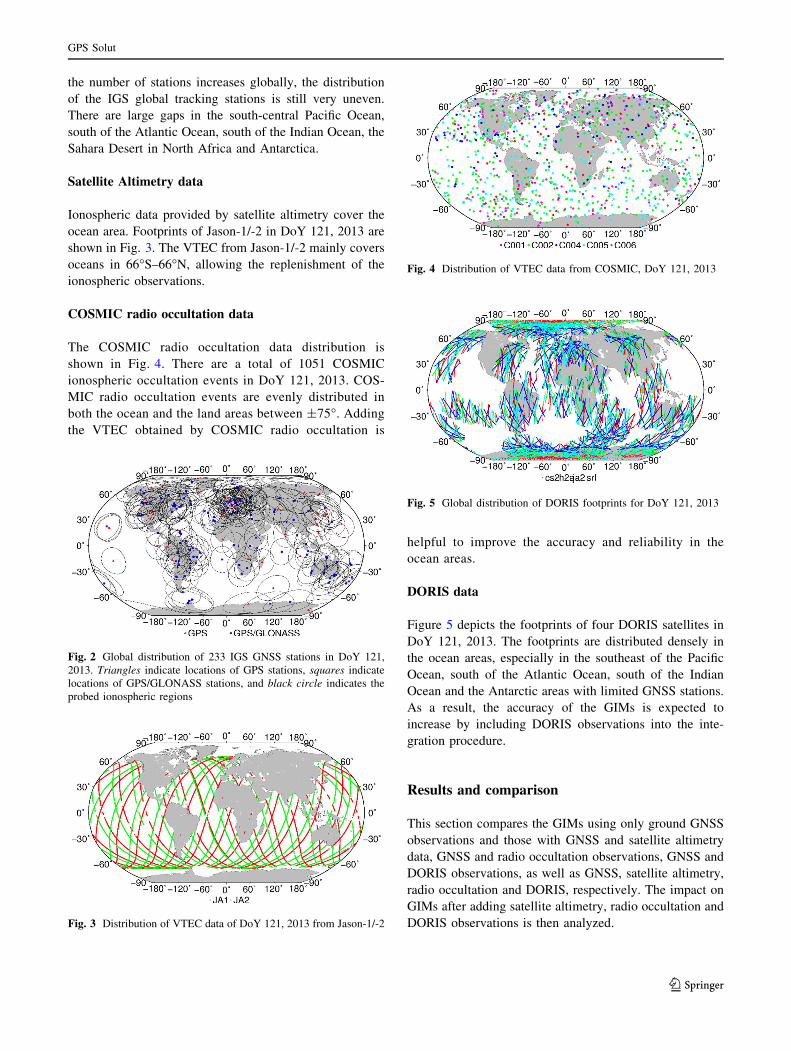
the number of stations increases globally, the distribution

of the IGS global tracking stations is still very uneven.

There are large gaps in the south-central Pacific Ocean,

south of the Atlantic Ocean, south of the Indian Ocean, the

Sahara Desert in North Africa and Antarctica.

Satellite Altimetry data

Ionospheric data provided by satellite altimetry cover the

ocean area. Footprints of Jason-1/-2 in DoY 121, 2013 are

shown in Fig. 3. The VTEC from Jason-1/-2 mainly covers

oceans in 66�S–66�N, allowing the replenishment of the

ionospheric observations.

COSMIC radio occultation data

The COSMIC radio occultation data distribution is

shown in Fig. 4. There are a total of 1051 COSMIC

ionospheric occultation events in DoY 121, 2013. COS-

MIC radio occultation events are evenly distributed in

both the ocean and the land areas between ±75�. Addingthe VTEC obtained by COSMIC radio occultation is

helpful to improve the accuracy and reliability in the

ocean areas.

DORIS data

Figure 5 depicts the footprints of four DORIS satellites in

DoY 121, 2013. The footprints are distributed densely in

the ocean areas, especially in the southeast of the Pacific

Ocean, south of the Atlantic Ocean, south of the Indian

Ocean and the Antarctic areas with limited GNSS stations.

As a result, the accuracy of the GIMs is expected to

increase by including DORIS observations into the inte-

gration procedure.

Results and comparison

This section compares the GIMs using only ground GNSS

observations and those with GNSS and satellite altimetry

data, GNSS and radio occultation observations, GNSS and

DORIS observations, as well as GNSS, satellite altimetry,

radio occultation and DORIS, respectively. The impact on

GIMs after adding satellite altimetry, radio occultation and

DORIS observations is then analyzed.

Fig. 2 Global distribution of 233 IGS GNSS stations in DoY 121,

2013. Triangles indicate locations of GPS stations, squares indicate

locations of GPS/GLONASS stations, and black circle indicates the

probed ionospheric regions

Fig. 3 Distribution of VTEC data of DoY 121, 2013 from Jason-1/-2

Fig. 4 Distribution of VTEC data from COSMIC, DoY 121, 2013

Fig. 5 Global distribution of DORIS footprints for DoY 121, 2013

GPS Solut

123

GIMs from GNSS

The final GIMs and error maps at 10:00 UT of DoY 121,

2013, calculated using GNSS-only data, are shown in

Fig. 6. The global distribution and variation of ionospheric

VTEC is represented well, and the ionospheric equatorial

anomaly is clearly shown. The estimation error in most

areas is low, but is significantly large in several regions

with sparsely distributed GNSS stations, indicating that the

model accuracy is related with data distribution density.

Accuracies are higher over the land areas, while lower in

the ocean areas, especially in the north and southeast of the

Pacific Ocean, south of the Atlantic Ocean and south of the

Indian Ocean near the South Pole. The estimation error in

these areas even reaches 8.5 TECU. Therefore, if GNSS-

only data are used to build GIMs, the uneven distribution of

stations may lead to lower accuracy and reliability in ocean

areas. The bottom panel shows the global distribution map

of GNSS ionospheric pierce point between 09:00 and

11:00 UT. Large gaps of IPPs exist in ocean and the other

areas, and the lack of observational data in these areas

directly leads to the significantly higher estimation error

than other regions in middle panel.

GIMs from GNSS and satellite altimetry

Figure 7 shows that VTEC changes greatly in the ocean

areas. VTEC decreases by about 11 TECU at (180�E, 0�N)and its vicinity, increases by 4 TECU in the South Pacific

Fig. 6 Final GIMs (top) and error maps (middle) at 10:00 UT of DoY

121, 2013 modeled by GNSS data and IPP global distribution

between 09:00 and 11:00 UT (bottom)

Fig. 7 Differences of VTEC (top) and estimation error (middle) at

10:00 UT of DoY 121, 2013 between those modeled with GNSS-only

data and those modeled with both GNSS and altimetry data, and the

footprints of satellite altimetry between 09:00 and 11:00 UT in DoY

121, 2013 obtained from Jason-1/-2 (bottom)

GPS Solut

123

region, and increases by 3 TECU in the South Atlantic

region. After adding satellite altimetry data, the overall

estimation error decreases, while increases in some low

accuracy regions are detectable. The largest reduction

reaches 5 TECU at (180�E, 0�N) and its vicinity. The

estimation error reduces 2–3 TECU in south of the Atlantic

Ocean. The differences of VTEC and estimation error

shown in Fig. 7 indicate that the accuracy in ocean areas is

improved by combining satellite altimetry data. The

improvement of accuracy coincides with the footprints of

satellite altimetry. The area with the reduction of the esti-

mation error is exactly the region with satellite altimetry

data coverage, and the area with the most significant esti-

mation error declination is exactly the region with most

densely distributed satellite altimetry data.

GIMs from GNSS and radio occultation

This section provides the differences between the GIMs

using only GNSS data and GIMs by integration of GNSS

data and radio occultation data. The comparison results of

VTEC and estimation error are illustrated in Fig. 8. As

shown, the VTEC changes (-0.3 to -0.45 TECU) after

adding radio occultation data are much smaller than the

changes after adding ocean altimetry data. The most sig-

nificant VTEC changes occur mainly in the ocean areas in

the southern hemisphere. For example, the VTEC increases

by 0.4 TECU in the South Pacific near 30�S due to the small

number and discrete distribution of COSMIC observations

with little effect on final results. The area with the most

significant VTEC and estimation error change corresponds

to the area with denser radio occultation data distribution

and lower number of ground GNSS tracking stations.

GIMs from GNSS and DORIS

The differences between VTEC and estimation error cal-

culated with GNSS-only data and with both GNSS and

DORIS data at 10:00 UT of DoY 121, 2013 are demon-

strated in Fig. 9. VTEC changes between -6.0 and 3.0

TECU by adding DORIS data. Accuracies of GIMs, espe-

cially in the southeast of the Pacific and the Antarctic areas,

are improved significantly with a decrease of over 5 TECU,

while insignificant changes are shown on land, reflecting

subtle effect on areas with dense GNSS observations.

Although the distribution of DORIS data in Europe, South

America and the Atlantic region is more dense, the VTEC

and estimation error changes are very small, because the

distribution of ground GNSS tracking stations and DORIS

observations is sparser in the regions. Most IPPs in the 2 h

are located at the ocean areas and the Antarctic. The accu-

racies of GIMs modeled with GNSS and DORIS data are

significantly improved in the ocean areas, while little or no

improvement can be detected on land in comparison with

GIMs modeled with GNSS-only data.

GIMs from GNSS, satellite altimetry, radio

occultation and DORIS

According to the analysis above, adding satellite altimetry,

radio occultation and DORIS data into the combination

procedure will presumably offer globally denser distribu-

tion for the observations, especially in the ocean areas.

Integrating multi-source data can make use of their

Fig. 8 Differences of VTEC (top) and estimation error (middle) at

10:00 UT of DoY 121, 2013 between those modeled with GNSS-only

data and those modeled with both GNSS and radio occultation, and

global COSMIC radio occultation distribution during 09:00–11:00 UT

(bottom)

GPS Solut

123

advantages and achieve more accurate GIMs. Figure 10

shows the differences of VTEC and estimation error

between models only with GNSS data and models devel-

oped using combination of multi-source data. VTEC

changes significantly from -11.0 to 5.0 TECU after multi-

source data integration, and the accuracy of GIMs is

improved significantly with a decrease of 5.5 TECU.

Comparison among Figs. 7, 8, 9 and 10 indicates that areas

with improved accuracies are largest when modeling GIMs

by the integration of GNSS, satellite altimetry, radio

occultation and DORIS. This result indicates that com-

bining data from more kinds of technique may help

achieving higher accuracy in larger areas.

Validation and analysis

Ocean altimetry and COSMIC radio occultation observa-

tions that are not involved in the modeling process are used

in this section to validate the accuracy of all results. The

weights and systematic error of various kinds of observa-

tions are also analyzed.

External accuracy test

The mean absolute error (MAE) is chosen as criterion to

evaluate the models. The expressions of MAE is,

MAE ¼ 1

N

X

N

i¼1

y0i � yi�

�

�

� ð10Þ

where y0i and yi are modelled values and observed values,

respectively, and N is the number of observations.

The VTEC obtained by Jason-1/-2 and COSMIC

satellites is treated as true value, and the modeled

VTEC at the same position is obtained by interpolating

from GIMs. Then, the difference between the two

(considering the bias of satellite altimetry and COS-

MIC) is calculated. Finally, MAE can be obtained by

(10).

Fig. 10 Differences of VTEC (top) and estimation error (bottom) at

10:00 UT of DoY 121, 2013 between those modeled with GNSS-only

data and those modeled with integration of GNSS, satellite altimetry,

radio occultation and DORIS

Fig. 9 Differences of VTEC (top) and estimation error (middle) at

10:00 UT of DoY 121, 2013 between those modeled with GNSS-only

data and those modeled with both GNSS and DORIS data, the global

distribution of IPPs of DORIS rays in 09:00–11:00 UT of DoY 121,

2013 (bottom)

GPS Solut

123

Validation with Jason-1/-2

Parts of the observations from Jason-1/-2 not involved in

modeling are used as the true value to validate the model.

The MAE of the two GIMs in each day is also calculated as

shown in Fig. 11. The GIMs using multi-source data with

Jason-1/-2 VTEC are better than that using only ground

GNSS data. The average for MAE of GIMs using multi-

source data with Jason-1/-2 within 31 days in May 2013 is

2.88 TECU and 2.90 TECU, respectively, and is 0.47

TECU (14.02 %) and 0.44 TECU (13.17 %) less than the

monthly average using only GNSS data. A smaller differ-

ence between GIMs using multi-source data and Jason-1/-2

original observations indicates that the accuracy of GIMs

using multi-source data in ocean regions is improved.

Validation with COSMIC

To further validate the accuracy of GIMs using multi-

source data, we use part of observations from five COS-

MIC satellites which are not involved in modeling as the

true value and calculate the MAE of the two GIMs in each

day. Figure 12 shows the difference between the MAE of

GIMs using multi-source data and those using only ground

GNSS data within 31 days. Most MAE differences are less

than zero, indicating that the GIMs using multi-source data

are closer to COSMIC original observations. The monthly

average of MAE of multi-source data is 0.09 TECU lower

than that of GNSS only.

Analysis of weights

In this study, when determining the precise weight of dif-

ferent kinds of observations using variance components

estimation, we treat the weight of GPS observations as a

constant that equals 1 and further determine the weights of

other observation techniques.

The statistical result of the weight of various observa-

tions in 31 days is shown in Table 1. The weight of

GLONASS is lowest, with the average of only 0.37 and

standard deviation of 0.03. Weights of Jason-1/-2 and five

COSMIC satellites are all close to 0.5, while the accuracy

120 125 130 135 140 145 1502.2

2.4

2.6

2.8

3.0

3.2

3.4

3.6

3.8

4.0

MAE

of J

ason

-1 (T

ECu)

DOY (2013)

G G+A+R+D

120 125 130 135 140 145 1502.2

2.4

2.6

2.8

3.0

3.2

3.4

3.6

3.8

4.0

MAE

of J

ason

-2 (T

ECu)

DOY (2013)

G G+A+R+D

Fig. 11 Distribution of MAE of GIMs using GNSS data and GIMs

using multi-source data in DoY 121–151, 2013

120 125 130 135 140 145 150-0.4

-0.3

-0.2

-0.1

0.0

0.1

0.2

ΔMAE

(TEC

u)

DOY (2013)

C001 C002 C004 C005 C006

Fig. 12 Differences between MAE of multi-source data and MAE of

ground GNSS data in DoY 121–151, 2013

Table 1 Statistics of weights of various observation in DoY

121–151, 2013. The weight of GPS is regarded as a constant and

equal to 1

Max Min Mean SD

GLONASS 0.41 0.31 0.37 0.03

JA1 0.66 0.39 0.48 0.07

JA2 0.63 0.38 0.48 0.06

C001 0.76 0.27 0.46 0.11

C002 0.58 0.32 0.43 0.07

C004 0.79 0.37 0.51 0.10

C005 0.51 0.33 0.40 0.05

C006 0.69 0.33 0.44 0.09

Cryosat-2 1.17 0.66 0.87 0.13

HY-2A 1.13 0.61 0.86 0.14

Jason-2 1.59 0.84 1.11 0.20

Saral 1.48 0.73 1.07 0.17

GPS Solut

123

of VTEC obtained by DORIS is highest. The average

weight of Cryosat-2 and HY-2A is close to 0.9, while the

weight of Jason-2 and Saral is larger than 1.

Analysis of bias

The bias of various techniques with respect to GNSS is

calculated in this section. The bias of every COSMIC

satellite in 1 day is treated as a constant. The bias of Jason-

1/-2 and DORIS satellite is treated as a constant within 2 h.

The monthly average and standard deviation of the bias at

every 2 h of each satellite are calculated.

The monthly average and standard deviation of systemic

bias of Jason-1/-2 satellite in every 2 h are shown in

Fig. 13. The monthly averages of bias of Jason-1 and

Jason-2 have a similar trend, with the maximum in

16:00 UT and the minimum in 06:00–08:00 UT. The

average of Jason-1 is about 0.95 TECU and that of Jason-2

is -3.08 TECU, showing that the average VTEC obtained

by Jason-1 is 0.95 TECU larger than the GPS VTEC, while

the VTEC obtained by Jason-2 is 3.08 TECU smaller than

the GPS VTEC.

The bias of 5 COSMIC satellites relative to the GPS

VTEC in DoY 121–151, 2013 is illustrated Fig. 14. The

bias of C001, C002, C005 and C006 changes slightly

within 31 days. The monthly averages are, respectively,

-2.99, -2.80, -2.90 and -2.92 TECU, indicating that

VTEC obtained by COSMIC is on average about 2.9

TECU smaller than GPS VTEC. The bias of C004 dur-

ing DoY 123–133 is significantly lower than on other

days, with an average of -4.71 TECU. But in the

remaining days, the bias of C004 is consistent with other

satellites.

The monthly average and standard deviation of bias of

corrected DORIS VTEC are shown in Fig. 15. The biases

of the four satellites are oscillating around zero. The mean

biases of Cryosat-2, HY-2A, Jason-2 and Saral are,

respectively, -0.03, -0.01, -0.10 and 0.12 TECU, indi-

cating that there is no significant bias between GPS VTEC

and the corrected DORIS VTEC.

Conclusions

In this study, the GIM models are established by integra-

tion of multi-source data such as GNSS, satellite altimetry,

radio occultation and DORIS data. The biases between

different data are considered and are estimated together

with ionospheric model parameters. The bias of each ocean

altimetry satellite and each DORIS satellite is treated as a

constant over 2 h, and the bias of each radio occultation

satellite in 1 day is also treated as a constant. According to

the accuracy differences of ionospheric data from different

systems, the Helmert variance component estimation is

used to obtain the weights of different types of

observations.

The effect on the accuracy of GIMs by integrating

satellite altimetry, radio occultation and DORIS data is

analyzed using observations on DoY 121–151, 2013. The

result shows that the estimation error decreases by 5.5

TECU after adding satellite altimetry, radio occultation and

DORIS data, and the accuracy of GIMs is improved sig-

nificantly in the ocean areas.

0 2 4 6 8 10 12 14 16 18 20 22

-5

-4

-3

-2

-1

0

1

2

3S

yste

m b

ias

(TE

Cu)

UT

Jason-1 Jason-2

Fig. 13 Monthly average of bias between the satellite altimetry

VTEC and GPS systems in DoY 121–151, 2013

120 125 130 135 140 145 150

-5.0

-4.5

-4.0

-3.5

-3.0

-2.5

-2.0

Syst

em b

ias

(TEC

u)

DOY (2013)

C001 C002 C004 C005 C006

Fig. 14 Bias between the VTEC obtained by COSMIC satellites and

GPS systems in DoY 121–151, 2013

GPS Solut

123

Since more and more satellites can offer ionospheric

observations and the accuracy of the ionospheric observa-

tions improves, multi-source ionospheric integration has

great potential to create higher-accuracy GIMs, especially in

the ocean areas where ground GNSS stations are inadequate.

Acknowledgments We thank CDDIS for providing GNSS and

DORIS observation data, CNES and NOAA for providing Jason-1

and Jason-2 GDR data, respectively, NOAA for providing ionosonde

data and CDAAC for providing COSMIC ‘‘ionprf’’ data. This study

was funded by the National Natural Science Foundation of China

(41404031) and Key Laboratory of Geo-informatics of State Bureau

of Surveying and Mapping (201420).

References

Alizadeh M, Schuh H, Todorova S, Schmidt M (2011) Global

ionosphere maps of VTEC from GNSS, satellite altimetry, and

Formosat-3/COSMIC data. J Geodesy 85(12):975–987

Auriol A, Tourain C (2010) DORIS system: the new age. Adv Space

Res 46(12):1484–1496

Brunini C, Meza A, Bosch W (2005) Temporal and spatial variability

of the bias between TOPEX- and GPS-derived total electron

content. J Geod 79(4–5):175–188

Chen P, Chen J (2014) The multi-source data fusion global

ionospheric modeling software—IonoGim. Adv Space Res

53(11):1610–1622

Chen P, Yao W, Zhu X (2015) Combination of ground-and space-

based data to establish a global ionospheric grid model. IEEE

Trans Geosci Remote Sens 53(2):1073–1081

Dettmering D, Schmidt M, Heinkelmann R, Seitz M (2011) Combi-

nation of different space-geodetic observations for regional

ionosphere modeling. J Geod 85(12):989–998

Feltens J (2003) The international GPS service (IGS) Ionosphere

working group. Adv Space Res 31(3):635–644

Fong C-J, Yen NL, Chu C-H, Yang S-K, Shiau W-T, Huang C-Y,

Chi S, Chen S-S, LiouY-A KuoY-H (2009) FORMOSAT-3/

COSMIC spacecraft constellation system, mission results, and

prospect for follow-on mission. Terr Atmos Ocean Sci

20:1–19

Hernandez-Pajares M, Juan JM, Sanz J, Orus R, Garcia-Rigo A,

Feltens J, Krankowski A (2009) The IGS VTEC maps: a reliable

source of ionospheric information since 1998. J Geodesy

83(3–4):263–275

Koch KR, Kusche J (2002) Regularization of geopotential determi-

nation from satellite data by variance components. J Geodesy

76(5):259–268

Li Z, Yuan Y, Li H, Ou J, Huo X (2012) Two-step method for the

determination of the differential code biases of COMPASS

satellites. J Geodesy 86(11):1059–1076

Mannucci AJ, Wilson BD, Yuan DN, Ho CH, Lindqwister UJ, Runge

TF (1998) A global mapping technique for GPS-derived

ionospheric total electron content measurements. Radio Sci

33(3):565–582

Mercier F, Cerri L, Berthias JP (2010) Jason-2 DORIS phase

measurement processing. Adv Space Res 45(12):1441–1454

Schaer S (1999) Mapping and predicting the earth’s ionosphere using

the Global Positioning System. Ph.D. thesis, Bern University,

Switzerland

Todorova S, Schuh H, Hobiger T (2007) Using the global navigation

satellite systems and satellite altimetry for combined global

ionosphere maps. Adv Space Res 42:727–736

Yuan YB (2002) Theory and method research of GPS-based

ionospheric monitoring and delay correction. Institute of

Geodesy and Geophysics, CAS, Wuhan

Zhang X, Tang L (2014) Daily global plasmaspheric maps derived

from cosmic GPS observations. IEEE Trans Geosci Remote Sens

52(10):6040–6046

-1.0

-0.5

0.0

0.5

1.0

Cryosat-2

Syst

em b

ias

(TEC

u) HY-2A

0 2 4 6 8 10 12 14 16 18 20 22 0 2 4 6 8 10 12 14 16 18 20 22-1.0

-0.5

0.0

0.5

1.0

Jason-2Sy

stem

bia

s (T

ECu)

UT

Saral

UT

Fig. 15 Monthly average of

systematic differences between

the DORIS VTEC and GPS

systems in DoY 121–151, 2013

GPS Solut

123

Peng Chen received the Ph.D.

degree in geodesy and survey-

ing engineering from Wuhan

University, Wuhan, China, in

2012. He is currently a Lecturer

with the College of Geomatics,

Xi’an University of Science and

Technology, Xi’an, China. His

main research interests include

global ionospheric modeling

using multisource geodesy

observations, 3-D ionospheric

tomography and ionospheric

anomaly analysis under abnor-

mal conditions.

Yibin Yao received the B.Sc.,

Master’s, and Ph.D. degrees in

geodesy and surveying engi-

neering from Wuhan University,

Wuhan, China, in 1997, 2000

and 2004, respectively. He is

currently a Professor with

Wuhan University. His main

research interests include global

navigation satellite system

ionospheric/atmospheric/meteo-

rological studies, theory and

method of surveying data pro-

cessing, and GPS/MET and high

precision GPS data processing.

Wanqiang Yao received the

Ph.D. degree from Chang’an

University, Xi’an, in 2004. He is

currently the Dean and a Pro-

fessor with the College of Geo-

matics, Xi’an University of

Science and Technology, Xi’an.

His research interests include 3S

integration and applications,

and remote sensing and geo-

graphical conditions

monitoring.

GPS Solut

123