House Price Indices from the 1984–1992MSA American Housing Surveys
44
Journal of Housing Research • Volume 6, Issue 3 439 © Fannie Mae 1995. All Rights Reserved. House Price Indices from the 1984–1992 MSA American Housing Surveys Thomas G. Thibodeau* Abstract This article reports residential real estate price indices computed from the Metropolitan Statis- tical Area American Housing Survey for 1984 through 1992. It extends the hedonic price indices reported earlier to metropolitan areas surveyed during those years. Price indices for owner- occupied housing and for rental housing services are computed using 1985 national average housing characteristics. Housing inflation rates are measured using Laspeyres, Paasche, and Fisher indices. The article provides (1) house price indices based on random samples of the entire housing stock rather than (nonrandom) samples of properties that sell one or more times; (2) indices that price a constant bundle of housing characteristics across the 44 metropolitan areas and over time; (3) indices for both house prices and housing inflation rates; (4) tenure-specific price indices for new housing, existing standard-quality housing, and substandard housing; and (5) an estimate of the gradual improvements in the nation’s housing stock. Keyword: hedonic house price indices Introduction Accurate measurement of house prices is important for a variety of reasons. Housing consumers, urban economists, and housing policy analysts require information on house prices when making housing consumption decisions, when modeling housing market behavior, and when evaluating the equity and efficiency implications of alternative government housing assistance programs. Constant-quality metropolitan-area house prices enable consumers to make comparisons across housing markets. Urban econo- mists use house price indices for many purposes: 1. To identify the determinants of spatial and temporal variation in house prices (Blackley and Follain 1987; Fortura and Kushner 1986; Guntermann and Norrbin 1987; Manning 1989; Ozanne and Thibodeau 1983) 2. To measure the rate of economic depreciation for housing (Hulten and Wykoff 1981; Malpezzi, Ozanne, and Thibodeau 1980, 1987; Randolph 1988; Shilling, Sirmans, and Dombrow 1991) * Thomas G. Thibodeau is Professor of Real Estate at the E. L. Cox School of Business, Southern Methodist University. This research was supported by Fannie Mae, the Housing and Household Economic Statistics Division of the U.S. Bureau of the Census, and the Folsom Institute for Development and Land Use Policy at the E. L. Cox School of Business at Southern Methodist University. The author thanks Daniel H. Weinberg for providing access to the data and a pleasant working environment. The opinions expressed are those of the author and do not necessarily represent the views of Fannie Mae, the Folsom Institute, or the Bureau of the Census. The author accepts responsibility for any errors in the article.
Transcript of House Price Indices from the 1984–1992MSA American Housing Surveys

House Price Indices from the 1984–1992 MSA American Housing Surveys 439Journal of Housing Research • Volume 6, Issue 3 439© Fannie Mae 1995. All Rights Reserved.
House Price Indices from the 1984–1992 MSA AmericanHousing Surveys
Thomas G. Thibodeau*
Abstract
This article reports residential real estate price indices computed from the Metropolitan Statis-tical Area American Housing Survey for 1984 through 1992. It extends the hedonic price indicesreported earlier to metropolitan areas surveyed during those years. Price indices for owner-occupied housing and for rental housing services are computed using 1985 national averagehousing characteristics. Housing inflation rates are measured using Laspeyres, Paasche, andFisher indices.
The article provides (1) house price indices based on random samples of the entire housing stockrather than (nonrandom) samples of properties that sell one or more times; (2) indices that pricea constant bundle of housing characteristics across the 44 metropolitan areas and over time;(3) indices for both house prices and housing inflation rates; (4) tenure-specific price indices fornew housing, existing standard-quality housing, and substandard housing; and (5) an estimate ofthe gradual improvements in the nation’s housing stock.
Keyword: hedonic house price indices
Introduction
Accurate measurement of house prices is important for a variety of reasons. Housingconsumers, urban economists, and housing policy analysts require information on houseprices when making housing consumption decisions, when modeling housing marketbehavior, and when evaluating the equity and efficiency implications of alternativegovernment housing assistance programs. Constant-quality metropolitan-area houseprices enable consumers to make comparisons across housing markets. Urban econo-mists use house price indices for many purposes:
1. To identify the determinants of spatial and temporal variation in house prices(Blackley and Follain 1987; Fortura and Kushner 1986; Guntermann and Norrbin1987; Manning 1989; Ozanne and Thibodeau 1983)
2. To measure the rate of economic depreciation for housing (Hulten and Wykoff 1981;Malpezzi, Ozanne, and Thibodeau 1980, 1987; Randolph 1988; Shilling, Sirmans,and Dombrow 1991)
* Thomas G. Thibodeau is Professor of Real Estate at the E. L. Cox School of Business, Southern MethodistUniversity. This research was supported by Fannie Mae, the Housing and Household Economic StatisticsDivision of the U.S. Bureau of the Census, and the Folsom Institute for Development and Land Use Policy atthe E. L. Cox School of Business at Southern Methodist University. The author thanks Daniel H. Weinbergfor providing access to the data and a pleasant working environment. The opinions expressed are those of theauthor and do not necessarily represent the views of Fannie Mae, the Folsom Institute, or the Bureau of theCensus. The author accepts responsibility for any errors in the article.

440 Thomas G. Thibodeau
3. To examine the influence of federal income taxes on tenure choice (Cooperstein1989; Cronin 1983; Grootaert and Dubois 1988; Herrin and Kern 1992; Lea andWasylenko 1983; Nicholson and Willis 1991; Woodward and Weicher 1989)
4. To measure property tax capitalization (Ihlanfeldt 1983; Ihlanfeldt and Boehm1983; Ihlanfeldt and Jackson 1982; King 1973)
5. To estimate models of housing search and household mobility (Boehm 1984; DeBoer1985)
6. To examine how households form their expectations of house value appreciation(Hamilton and Schwab 1985)
7. To measure housing inflation and rates of return on housing (Crone 1988; Kiel andCarson 1990; Manning 1986; Ozanne 1981; Pollakowski, Stegman, and Rohe 1991)
8. To measure housing quality (Wieand 1983)
9. To test for bias in homeowners’ estimates of house value (Follain and Malpezzi 1981)
10. To test for racial discrimination in the housing market (King and Mieszkowski 1973)
11. To quantify the influence of externalities on residential properties (Grether andMieszkowski 1974, 1980; Li and Brown 1980; Mieszkowski and Saper 1978; Thibodeau1990)
12. To evaluate the effect of alternative mortgage instruments on house prices (Agarwaland Phillips 1983, 1984)
Finally, housing policy analysts use house price indices to examine the efficiency ofgovernment housing assistance programs (Jackson and Mohr 1986; Olsen and Barton1983; Reeder 1985; Sa-Aadu 1984a, 1984b; Schwab 1985), to assess housing affordability(Linneman and Megbolugbe 1992), and to study how rent control affects housing markets(Marks 1984; Olsen 1972; Willis, Malpezzi, and Tipple 1990).
This article reports house price indices using data obtained from the 44 metropolitanstatistical areas (MSAs) surveyed in the MSA American Housing Survey (AHS) for 1984through 1992. Since 1984, the U.S. Bureau of the Census has conducted detailed surveysof the housing stock in 44 metropolitan areas. Metropolitan areas are surveyed in a 4-yearcycle, with 11 areas surveyed each year. Each metropolitan AHS uses a random sampleof about 3,200 residential dwellings. The data are collected between April and October ofthe survey year. Each survey questionnaire contains more than 300 questions ondwelling and occupant characteristics.
House price indices are computed by the hedonic index method. This statistical procedureuses regression analysis to explain variation in rents and house values using propertystructural and neighborhood characteristics (dwelling size, age, location, etc.). Separate

House Price Indices from the 1984–1992 MSA American Housing Surveys 441
regression equations are estimated for specified owner-occupied1 and for specifiedrenter-occupied2 properties in each of the 99 metropolitan surveys (9 survey years,11 metropolitan areas per year).
Tenure-specific house prices are computed by predicting the market rent or market valuefor a constant-quality dwelling. Separate averages are used to price dwelling character-istics for renter- and owner-occupied properties. For renter-occupied dwellings, thepredicted rent measures the price of one month of rental housing services. Because thehousing characteristics that are priced are held constant across all surveys, differencesin predicted rents reflect differences in the price of rental housing services. The predictedrents measure shelter rent by excluding utility payments. For owner-occupied units, thepredicted house value measures the price of a constant-quality house.
Within each metropolitan area, house price indices are computed for the entire housingstock as well as for three distinct points in the dwelling quality distribution: (1) forsubstandard housing (according to a definition of substandard housing previously usedby the U.S. Department of Housing and Urban Development [HUD]), (2) for new housing(housing less than three years old and not substandard), and (3) for existing standard-quality housing (everything else). The housing characteristics that are priced arenational average housing characteristics for dwellings in places with populations exceed-ing 100,000. Average dwelling characteristics were computed from the 1985 NationalAmerican Housing Survey, a random sample of the nation’s housing stock.
The hedonic specification and the housing markets examined here are similar to thoseused earlier. Thibodeau (1989, 1992) computed tenure-specific house price indices for60 metropolitan areas surveyed in the Standard Metropolitan Statistical Area AnnualHousing Survey between 1974 and 1983. Each metropolitan area was surveyed repeat-edly in a three- or four-year cycle, yielding 164 metropolitan surveys.
In 1984, the U.S. Bureau of the Census redesigned the metropolitan Annual HousingSurvey, renaming it the American Housing Survey and changing it in two significantways. First, the metropolitan-area coverage was reduced from 60 areas to 44: Sixteenmetropolitan areas were dropped from the survey, some metropolitan areas werecombined, and two metropolitan areas—San Jose, CA, and Tampa, FL—were added.Second, the Census Bureau extended the geographic boundaries for approximately two-thirds of the metropolitan areas, to incorporate suburban counties, and relabeled themmetropolitan statistical areas. The boundaries for the Atlanta metropolitan area, forexample, were expanded to include an additional 13 suburban counties. The countiesadded to metropolitan areas in the 1984 redesign have been deleted in this study to makethe housing markets examined here comparable to those in the pre-1984 surveys.
The constant-quality house price indices are used to measure housing inflation rates.Three indices for measuring inflation are computed: a Laspeyres index, which measuresthe price change that occurred in the beginning period’s bundle of housing characteris-tics; a Paasche index, which measures the price change that occurred in the ending
1 A specified owner-occupied unit is a single-family dwelling on less than 10 acres with no commercial, medical,or dental offices on the property.
2 The specified renter-occupied category excludes single-family dwellings on 10 acres or more.
442 Thomas G. Thibodeau
period’s bundle of housing characteristics; and a Fisher index, which is the geometricmean of the Laspeyres and Paasche indices. Finally, a house quality index assesses thegradual improvements taking place in the nation’s housing stock.
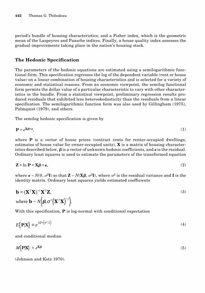
The Hedonic Specification
The parameters of the hedonic equations are estimated using a semilogarithmic func-tional form. This specification regresses the log of the dependent variable (rent or housevalue) on a linear combination of housing characteristics and is selected for a variety ofeconomic and statistical reasons. From an economic viewpoint, the semilog functionalform permits the dollar value of a particular characteristic to vary with other character-istics in the bundle. From a statistical viewpoint, preliminary regression results pro-duced residuals that exhibited less heteroskedasticity than the residuals from a linearspecification. The semilogarithmic function form was also used by Gillingham (1975),Palmquist (1979), and others.
The semilog hedonic specification is given by
PX= +e � �, (1)
where P is a vector of house prices (contract rents for renter-occupied dwellings,estimates of house value for owner-occupied units), X is a matrix of housing character-istics described below, � is a vector of unknown hedonic coefficients, and � is the residual.Ordinary least squares is used to estimate the parameters of the transformed equation
Z P X= = +ln ,� � (2)
where � ~ N(0, �2I) so that Z ~ N(X�, �2I), where �2 is the residual variance and I is theidentity matrix. Ordinary least squares yields estimated coefficients
b X X X Z= −( ) ,1T T (3)
where ~b X XN T�, .σ 2 1( )( )−
With this specification, P is log-normal with conditional expectation
E eX
P X{ } = +( )β σ2 2 (4)
and conditional median
M ePX X{ } = � (5)
(Johnson and Kotz 1970).

House Price Indices from the 1984–1992 MSA American Housing Surveys 443
The dependent variable for the renter equation is the log of the tenant-reported contractrent. The dependent variable for the owner-occupied equation is usually the log of theowner’s estimate of the market value of the property.3 If the property sold within theprevious year, the dependent variable is the log of the transaction price.
Several housing characteristics are included in X:
1. Structural characteristics of the dwelling (dummy variables for the number ofbathrooms, bedrooms, and other rooms; number of units in the structure; dwellingage, age squared, age cubed; and, for owner-occupied dwellings, dummy variablesfor the presence of a garage or a basement)
2. Dwelling equipment (type of heating and air conditioning)
3. Dwelling quality (presence of structural defects, frequency of equipment break-downs, etc.)
4. Neighborhood quality (resident’s opinion of the neighborhood, whether the residentrecently observed rats in the building, etc.)
5. Race of the household head4
6. Contract conditions that may influence house prices (number of persons per room,5
occupant’s length of tenure,6 length of tenure squared, and, for renters, whetherpayments for various utilities are included in the contract rent). Because MSA AHSinformation is collected throughout the survey year, the hedonic specification alsoincludes dummy variables for the month of interview. All variables used in thehedonic equations are defined in table 1. Finally, for most MSAs, the AHS identifiesproperties located in various counties included in the metropolitan area. Thehedonic specification includes county dummy variables whenever the AHS identi-fies county locations. The areas surveyed in the 1974–92 metropolitan AHS, thesurvey years, the counties added in the 1984 redesign, and the location variablesused in the hedonic equations are summarized in table 2.
3 Recently, Goodman and Ittner (1992) reported that homeowners systematically overestimate the value oftheir homes. Robins and West (1977) and Ihlanfeldt and Martinez-Vazquez (1986) had similar findings, butother analysts have had conflicting findings. Follain and Malpezzi (1981) reported that homeowners whoowned their dwellings for long periods tended to underestimate market value. Similarly, Wolters and Woltman(1974) concluded that homeowners underestimated the market value of their properties by 3 percent in the1970 census. Finally, Kish and Lansing (1954) and Kain and Quigley (1972) compared homeowners’ estimateswith professional appraisers’ estimates and concluded that homeowners had unbiased estimates.
4 The race of the head of household serves as a proxy for neighborhood conditions. It would certainly bepreferable to have more direct information on the percentage of the neighborhood that is minority or data onthe dwelling’s census tract, but this information is not available in the AHS.
5 A density variable is included because household density influences the rate of economic depreciation—thegreater the utilization rate, the higher the depreciation rate. Landlords compensate by charging higher rents.
6 Length-of-tenure variables are included in the renter equation to capture discounts available to long-termresidents. They are included in the owner equation to accommodate the potential bias associated with theowner’s estimate of house value (Follain and Malpezzi 1981).

444 Thomas G. Thibodeau
Table 1. Hedonic Equation Variable Definitions
Variable Tenure Definition
I. Dependent variables
LNRENT Renters Log of monthly contract rent
LNVALUE Owners Log of reported selling price if property sold within last12 months; otherwise, log of the owner’s house valueestimate
II. Structural variables
Bathrooms
BATHS10 Both One full bathroom (a room with a flush toilet,(omitted) bathtub or shower, and sink)
BATHS15 Both One-and-a-half bathrooms (a half bath is a room witheither a flush toilet or a bathtub or shower but not thefacilities of a full bath)
BATHS20 Owners Two full baths or two-and-a-half baths
BATHS2P Renters Two or more full baths
BATHS3P Owners Three or more full baths
Bedrooms
BDRMS0 Renters No bedrooms
BDRMS1 Both One bedroom for renter equation; either no bedrooms orone bedroom for owner equation
BDRMS2 Both Two bedrooms(omitted)
BDRMS3 Both Three bedrooms
BDRMS4 Owners Four bedrooms
BDRMS4P Renters 0.25 times the number of bedrooms for units with four ormore bedrooms
BDRMS5P Owners 0.20 times the number of bedrooms for units with five ormore bedrooms
Other rooms
OROOMS1 Renters One other room
OROOMS2 Both Two other rooms(omitted)
OROOMS3 Both Three other rooms
OROOMS4 Owners Four other rooms
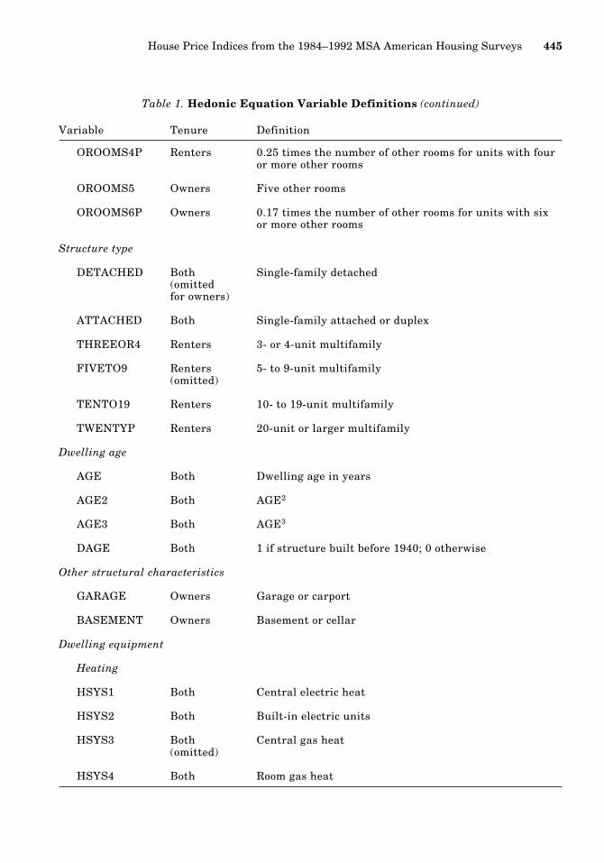
House Price Indices from the 1984–1992 MSA American Housing Surveys 445
Table 1. Hedonic Equation Variable Definitions (continued)
Variable Tenure Definition
OROOMS4P Renters 0.25 times the number of other rooms for units with fouror more other rooms
OROOMS5 Owners Five other rooms
OROOMS6P Owners 0.17 times the number of other rooms for units with sixor more other rooms
Structure type
DETACHED Both Single-family detached(omittedfor owners)
ATTACHED Both Single-family attached or duplex
THREEOR4 Renters 3- or 4-unit multifamily
FIVETO9 Renters 5- to 9-unit multifamily(omitted)
TENTO19 Renters 10- to 19-unit multifamily
TWENTYP Renters 20-unit or larger multifamily
Dwelling age
AGE Both Dwelling age in years
AGE2 Both AGE2
AGE3 Both AGE3
DAGE Both 1 if structure built before 1940; 0 otherwise
Other structural characteristics
GARAGE Owners Garage or carport
BASEMENT Owners Basement or cellar
Dwelling equipment
Heating
HSYS1 Both Central electric heat
HSYS2 Both Built-in electric units
HSYS3 Both Central gas heat(omitted)
HSYS4 Both Room gas heat

446 Thomas G. Thibodeau
Table 1. Hedonic Equation Variable Definitions (continued)
Variable Tenure Definition
HSYS5 Both Central oil heat
HSYS6 Both Other heating system not specified above (includes unitsthat have no heating equipment as well as dwellingsheated with solar heat, coal, or firewood)
Air conditioning
ACSYS1 Both No air conditioning
ACSYS2 Both At least one room air conditioner but no central airconditioning
ACSYS3 Both Central air conditioning(omitted)
Dwelling quality
BLDGPROB Both Building problems (1 if the unit has two or more of thefollowing problems: basement leaks, roof leaks, opencracks or holes in walls or ceilings, holes in floor, orbroken plaster or peeling paint over an area exceedingone square foot; 0 otherwise)
HALLPROB Renters Public hallway problems (1 if unit is in a multifamilybuilding and has at least two of the following problems:absence of light fixtures in public halls, hazardous stepson common stairs, or stair railings not firmly attached;0 otherwise)
LACKFEAT Both Lack of important features (1 if unit has any of thefollowing deficiencies: lacks complete plumbing; lackscomplete kitchen facilities; sewer system is a chemicaltoilet, privy, outhouse, facilities in another structure, orsome other sewage/toilet facilities; wiring in house notconcealed; or some rooms lack working electrical outlets;0 otherwise)
BREAKDWN Both Multiple equipment breakdowns (1 if unit had any of thefollowing equipment breakdowns: two or more waterbreakdowns lasting six hours or more, two or more flushtoilet breakdowns lasting six hours or more, two or morepublic sewer breakdowns lasting six hours or more, orfuses or circuit breakers blew two or more times withinthe last 90 days; 0 otherwise)
Neighborhood variables
Respondent’s overall opinion of neighborhood
EXCLNBHD Both The respondent is asked to rate the overall quality of theneighborhood between 1 (poor) and 10 (excellent). Thevariable equals 1 if the respondent ranks the neighbor-hood a 9 or a 10 and equals 0 otherwise.

House Price Indices from the 1984–1992 MSA American Housing Surveys 447
Table 1. Hedonic Equation Variable Definitions (continued)
Variable Tenure Definition
GOODNBHD Both The variable equals 1 if the respondent ranks theneighborhood between 4 and 8 and equals 0 otherwise.
FAIRPOOR Both The variable equals 1 if the respondent ranks the(omitted) neighborhood below 4 and equals 0 otherwise.
Other neighborhood variables
SEERATS Both The variable equals 1 if the respondent observed signs ofrats or mice in the building during the last 90 days andequals 0 otherwise.
ABANDON Both The variable equals 1 if the census enumerator observedabandoned buildings on the street and equals 0otherwise.
LITTER Both The variable equals 1 if respondents are so disturbed bytrash, litter, or junk in the streets (roads), on empty lots,or on properties in the neighborhood that they want tomove and equals 0 otherwise.
CRIME Both Street crime is a problem. The variable equals 1 ifrespondents report that street or neighborhood crime isso disturbing that they want to move and equals0 otherwise.
NOISE Both Street noise is a problem. The variable equals 1 ifrespondents report that street noise is so bad that theywant to move and equals 0 otherwise.
BLACK Both The variable equals 1 if the household head is black andequals 0 otherwise.
HISPAN Both The variable equals 1 if the household head is Hispanicand equals 0 otherwise.
Contract conditions
CROWDS Both Number of persons per room
LOT Both Resident’s length of tenure (difference between the dateof the interview and the date the head of the householdmoved in). Interval midpoints are used for dates re-ported as intervals. The year 1940 is assigned to theopen-ended category (household head moved in before1949).
LOT2 Both LOT2
DLOT Owners The variable equals 1 if the head of household movedinto the dwelling before 1949 and equals 0 otherwise.
EHEATINC Renters The variable equals 1 if payment for electric heat isincluded in contract rent and equals 0 otherwise.

448 Thomas G. Thibodeau
Table 1. Hedonic Equation Variable Definitions (continued)
Variable Tenure Definition
OELECINC Renters The variable equals 1 if payment for electricity isincluded in contract rent but electricity is not used toprovide space heat and equals 0 otherwise.
GHEATINC Renters The variable equals 1 if payment for gas heat is includedin contract rent and equals 0 otherwise.
OILINC Renters The variable equals 1 if payment for oil heat is includedin contract rent and equals 0 otherwise.
OTHERINC Renters The variable equals 1 if payment for other utilities (wateror gas when gas is not used to provide space heat) areincluded in contract rent and equals 0 otherwise.
Month of interview
MONTHj Both The variable equals 1 if the dwelling was surveyed inj = 2, . . . , 9 January or February (for j = 2) and 0 otherwise; March
for j = 3, etc. The survey is conducted from Januarythrough September. For these hedonic equations, Janu-ary and February were combined into one period. Onecategory must be omitted to avoid perfect multico-linearity. The omitted interview month is June.

House Price Indices from the 1984–1992 MSA American Housing Surveys 449T
able
2.
Met
rop
oli
tan
AH
S G
eog
rap
hy
, 19
74–1
992
Met
ropo
lita
n A
rea
Pos
t-19
83 S
urv
eys
Add
ed C
oun
ties
/Cit
ies
Hed
onic
Loc
atio
n V
aria
bles
Alb
any-
Sch
enec
tady
-Tro
y, N
Y (
SM
SA
)N
ot s
urv
eyed
All
ento
wn
-Bet
hle
hem
-Eas
ton
, P
A (
SM
SA
)N
ot s
urv
eyed
An
ahei
m–S
anta
An
a, C
A (
PM
SA
)19
86,
1990
Non
eA
nah
eim
Cit
y (i
nte
rcep
t)S
anta
An
a C
ity
Gar
den
Gro
ve C
ity
Bal
ance
of
Ora
nge
Co.
Atl
anta
, G
A (
MS
A)
1987
, 19
91C
her
okee
Co.
Cla
yton
Co.
For
syth
Co.
Gw
inn
ett
Co.
Pau
ldin
g C
o.A
tlan
ta C
ity
in D
e K
alb
Co.
Bar
r ow
Co.
Atl
anta
Cit
y in
Fu
lton
Co.
Dou
glas
Co.
(in
ter c
ept)
Wal
ton
Co.
Bal
anc e
of
De
Kal
b C
o.R
ock
dale
Co.
Bal
anc e
of
Fu
lton
Co.
New
ton
Co.
Cob
b C
o.C
owet
a C
o.F
ayet
te C
o.H
enry
Co.
Spa
ldin
g C
o.B
utt
s C
o.
Bal
tim
ore,
MD
(M
SA
)19
87,
1991
Qu
een
An
ne’
s C
o.C
arr o
ll C
o.H
arfo
r d C
o.H
owar
d C
o.B
alti
mor
e C
ity
(in
ter c
ept)
Bal
ance
of
Bal
tim
ore
Co.
An
ne
Aru
nde
l C
o.
Bir
min
gham
, A
L (
MS
A)
1984
, 19
88,
1992
Blo
un
t C
o.S
hel
by C
o.S
t. C
lair
Co.
Bir
min
gham
Cit
y (i
nte
r cep
t)B
alan
ce o
f Je
ffer
son
Co.
Wal
ker
Co.

450 Thomas G. ThibodeauT
able
2.
Met
rop
oli
tan
AH
S G
eog
rap
hy
, 19
74–1
992
(con
tin
ued
)
Met
ropo
lita
n A
rea
Pos
t-19
83 S
urv
eys
Add
ed C
oun
ties
/Cit
ies
Hed
onic
Loc
atio
n V
aria
bles
Bos
ton
, M
A-N
H (
CM
SA
)19
85,
1989
, 19
93H
ills
boro
ugh
Co.
, N
HE
ssex
Co.
, M
AR
ock
ingh
am C
o.,
NH
Mid
dles
ex C
o.,
MA
(pa
rt)
Wor
cest
er C
o.,
MA
Nor
folk
Co.
, M
A (
part
)B
rist
ol C
o.,
MA
Ply
mou
th C
o.,
MA
(pa
rt)
Su
ffol
k C
o.,
MA
(pa
rt)
Bos
ton
Cit
y, M
A (
inte
rcep
t)C
ambr
idge
Cit
y, M
AB
rock
ton
Cit
y, M
A
Bu
ffal
o, N
Y (
CM
SA
)19
84,
1988
Non
eN
iaga
ra C
o.B
uff
alo
Cit
y (i
nte
rcep
t)B
alan
ce o
f E
rie
Co.
Nia
gara
Fal
ls C
ity
Ch
icag
o, I
L (
PM
SA
)19
87,
1991
Ken
dall
Co.
Kan
e C
o.G
r un
dy C
o.L
ake
Co.
Wil
l C
o.C
hic
ago
Cit
y (i
nte
r cep
t)B
alan
ce o
f C
ook
Co.
Du
Pag
e C
o.
Cin
c in
nat
i, O
H-K
Y-I
N (
PM
SA
)19
86,
1990
Non
eC
lerm
ont
Co.
, O
HW
arre
n C
o.,
OH
Boo
ne
Co.
, K
YC
ampb
ell
Co.
, K
YC
inc i
nn
ati
Cit
y, O
H (
inte
r cep
t)B
alan
ce o
f H
amil
ton
Co.
, O
HK
ento
n C
o.,
KY
Cle
vela
nd,
OH
(P
MS
A)
1984
, 19
88,
1992
Non
eG
eau
ga C
o.M
edin
a C
o.C
leve
lan
d C
ity
(in
ter c
ept)
Bal
ance
of
Cu
yah
oga
Co.
Lak
e C
o.

House Price Indices from the 1984–1992 MSA American Housing Surveys 451T
able
2.
Met
rop
oli
tan
AH
S G
eog
rap
hy
, 19
74–1
992
(con
tin
ued
)
Met
ropo
lita
n A
rea
Pos
t-19
83 S
urv
eys
Add
ed C
oun
ties
/Cit
ies
Hed
onic
Loc
atio
n V
aria
bles
Col
orad
o S
prin
gs,
CO
(S
MS
A)
Not
su
rvey
ed
Col
um
bus,
OH
(M
SA
)19
87,
1991
Un
ion
Co.
Del
awar
e C
o.L
ick
ing
Co.
Lic
kin
g C
o.M
adis
on C
o.P
ick
away
Co.
Fai
rfie
ld C
o.C
olu
mbu
s C
ity
(in
terc
ept)
Bal
ance
of
Fra
nk
lin
Co.
Dal
las,
TX
(P
MS
A)
1985
, 19
89N
one
Den
ton
Co.
Ell
is C
o.D
alla
s C
ity
(in
ter c
ept)
Bal
anc e
of
Dal
las
Co.
Col
lin
Co.
Den
ver ,
CO
(C
MS
A)
1986
, 19
90D
ougl
as C
o.A
dam
s C
o.B
ould
er C
o.D
enve
r C
ity
(in
ter c
ept)
Jeff
erso
n C
o.A
rapa
hoe
Co.
Det
r oit
, M
I (P
MS
A)
1985
, 19
89L
apee
r C
o.M
acom
b C
o.S
t. C
lair
Co.
Oak
lan
d C
o.L
ivin
gsto
n C
o.D
etr o
it C
ity
(in
ter c
ept)
Mon
roe
Co.
Bal
ance
of
Way
ne
Co.
For
t W
orth
, T
X (
PM
SA
)19
85,
1989
Par
ker
Co.
Joh
nso
n C
o.F
ort
Wor
th C
ity
(in
ter c
ept)
Ar l
ingt
on C
ity
Bal
ance
of
Tar
r an
t C
o.

452 Thomas G. ThibodeauT
able
2.
Met
rop
oli
tan
AH
S G
eog
rap
hy
, 19
74–1
992
(con
tin
ued
)
Met
ropo
lita
n A
rea
Pos
t-19
83 S
urv
eys
Add
ed C
oun
ties
/Cit
ies
Hed
onic
Loc
atio
n V
aria
bles
Gra
nd
Rap
ids,
MI
(SM
SA
)N
ot s
urv
eyed
Har
tfor
d, C
T (
CM
SA
)19
87,
1991
Lit
chfi
eld
Co.
Har
tfor
d C
ity
(in
terc
ept)
New
Lon
don
Co.
Mid
dles
ex C
o. (
part
)T
olla
nd
Co.
(pa
rt)
New
Bri
tain
Cit
yB
rist
ol C
ity
Bal
ance
of
Har
tfor
d C
o.
Hon
olu
lu,
HI
(SM
SA
)N
ot s
urv
eyed
Hou
ston
, T
X (
PM
SA
)19
87,
1991
Wal
ler
Co.
For
t B
end
Co.
Mon
tgom
ery
Co.
Hou
ston
Cit
y (i
nte
r cep
t)B
alan
c e o
f H
arr i
s C
o.B
r azo
r ia
Co.
Indi
anap
olis
, IN
(M
SA
)19
84,
1988
, 19
92N
one
Boo
ne
Co.
Han
cock
Co.
Hen
dric
ks
Co.
Mor
gan
Co.
Sh
elby
Co.
Indi
anap
olis
Cit
y (i
nte
r cep
t)B
alan
ce o
f M
ario
n C
o.H
amil
ton
Cit
yJo
hn
son
Co.
Kan
sas
Cit
y, M
O-K
S (
CM
SA
)19
86,
1990
Ray
Co.
, M
OC
ass
Co.
, M
OL
eave
nw
orth
Co.
, K
SK
ansa
s C
ity
in C
lay
Co.
, M
OL
afay
ette
Co.
, M
OK
ansa
s C
ity
in P
latt
e C
o.,
MO
Mia
mi
Co.
, K
SJo
hn
son
Co.
, K
SK
ansa
s C
ity
in W
yan
dott
e C
o.,
KS

House Price Indices from the 1984–1992 MSA American Housing Surveys 453T
able
2.
Met
rop
oli
tan
AH
S G
eog
rap
hy
, 19
74–1
992
(con
tin
ued
)
Met
ropo
lita
n A
rea
Pos
t-19
83 S
urv
eys
Add
ed C
oun
ties
/Cit
ies
Hed
onic
Loc
atio
n V
aria
bles
Kan
sas
Cit
y in
Jac
kso
n C
o.,
MO
(in
terc
ept)
Bal
ance
of
Wya
ndo
tte
Co.
, K
SB
alan
ce o
f Ja
ckso
n C
o.,
MO
Bal
ance
of
Cla
y C
o.,
MO
Bal
ance
of
Pla
tte
Co.
, M
O
Las
Veg
as,
NV
(S
MS
A)
Not
su
rvey
ed
Los
An
gele
s–L
ong
Bea
ch,
CA
(P
MS
A)
1985
, 19
89N
one
Los
An
gele
s C
ity
(in
terc
ept)
Lon
g B
eac h
Cit
yB
alan
c e o
f L
os A
nge
les
Co.
Lou
isvi
lle,
KY
-IN
(S
MS
A)
Not
su
r vey
ed
Mad
ison
, W
I (S
MS
A)
Not
su
r vey
ed
Mem
phis
, T
N-A
R-M
S (
MS
A)
1984
, 19
88,
1992
Tip
ton
Co.
, T
NC
r itt
ende
n C
o.,
AR
DeS
oto
Co.
, M
SM
emph
is C
ity,
TN
(in
ter c
ept)
Bal
ance
of
Sh
elby
Co.
, T
N
Mia
mi–
For
t L
aude
rdal
e, F
L (
CM
SA
)19
86,
1990
Bro
war
d C
o.M
iam
i C
ity
(in
ter c
ept)
Bal
ance
of
Dad
e C
o.
Mil
wau
kee
, W
I (P
MS
A)
1984
, 19
88N
one
Oza
uk
ee C
o.W
ash
ingt
on C
o.M
ilw
auk
ee C
ity
(in
ter c
ept)
Wau
kes
ha
Co.
Bal
ance
of
Mil
wau
kee
Co.
Min
nea
poli
s–S
t. P
aul,
MN
-WI
(MS
A)
1985
, 19
89Is
anti
Co.
, M
NA
nok
a C
o.,
MN
Ch
isag
o C
o.,
MN
Dak
ota
Co.
, M
NW
r igh
t C
o.,
MN
Was
hin
gton
Co.
, M
NS
t. C
r oix
Co.
, W
IM
inn
eapo
lis
Cit
y, M
N (
inte
r cep
t)

454 Thomas G. ThibodeauT
able
2.
Met
rop
oli
tan
AH
S G
eog
rap
hy
, 19
74–1
992
(con
tin
ued
)
Met
ropo
lita
n A
rea
Pos
t-19
83 S
urv
eys
Add
ed C
oun
ties
/Cit
ies
Hed
onic
Loc
atio
n V
aria
bles
Car
ver
Co.
, M
NS
t. P
aul
Cit
y, M
NS
cott
Co.
, M
NB
alan
ce o
f H
enn
epin
Co.
, M
NB
alan
ce o
f R
amse
y C
o.,
MN
New
Orl
ean
s, L
A (
MS
A)
1986
, 19
90S
t. J
ohn
th
e B
apti
st P
aris
hS
t. B
ern
ard
Par
ish
St.
Ch
arle
s P
aris
hN
ew O
rlea
ns
Cit
y (i
nte
rcep
t)Je
ffer
son
Par
ish
St.
Tam
man
y P
aris
h
New
Yor
k–N
assa
u–S
uff
olk
, N
Y19
87,
1991
Ora
nge
Co.
Wes
tch
este
r C
o.(P
MS
A)
Pu
tnam
Co.
New
Yor
k C
ity
in B
ron
x C
o.N
ew Y
ork
Cit
y in
Kin
gs C
o. (
inte
rcep
t)N
ew Y
ork
Cit
y in
Qu
een
s C
o.N
ew Y
ork
Cit
y in
Ric
hm
ond
Co.
Nas
sau
Co.
Su
ffol
k C
o.
New
ark
–Nor
thea
ster
n19
87,
1991
Par
t of
nor
ther
n N
ew J
erse
yN
ewar
k C
ity
(in
ter c
ept)
New
Jer
sey,
NJ
(PM
SA
)H
uds
on C
o.M
orr i
s C
o.Je
rsey
Cit
yB
alan
ce o
f E
ssex
Co.
Hu
nte
rdon
Co.
Som
erse
t C
o.M
iddl
esex
Co.
Mon
mou
th C
o.O
cean
Co.
New
por t
New
s–H
ampt
on,
VA
1984
, 19
88,
1992
Par
t of
Nor
folk
–Vir
gin
iaN
ewpo
r t N
ews
Cit
y (i
nte
r cep
t)(S
MS
A)
Bea
ch–N
ewpo
r t N
ews
MS
AH
ampt
on C
ity
Bal
ance
of
Yor
k C
o.

House Price Indices from the 1984–1992 MSA American Housing Surveys 455T
able
2.
Met
rop
oli
tan
AH
S G
eog
rap
hy
, 19
74–1
992
(con
tin
ued
)
Met
ropo
lita
n A
rea
Pos
t-19
83 S
urv
eys
Add
ed C
oun
ties
/Cit
ies
Hed
onic
Loc
atio
n V
aria
bles
Nor
folk
–Vir
gin
ia B
each
–19
84,
1988
, 19
92Ja
mes
Cit
y C
o.N
orfo
lk C
ity
(in
terc
ept)
New
port
New
s, V
A (
MS
A)
Glo
uce
ster
Co.
Vir
gin
ia B
each
Cit
yW
illi
amsb
urg
Cit
yN
ewpo
rt N
ews
Cit
yS
uff
olk
Cit
yS
uff
olk
Cit
yC
hes
apea
ke
Cit
yP
orts
mou
th C
ity
Por
tsm
outh
Cit
yH
ampt
on C
ity
Nor
folk
Cit
yC
hes
apea
ke
Cit
yV
irgi
nia
Bea
ch C
ity
Yor
k C
o.
Ok
lah
oma
Cit
y, O
K (
MS
A)
1984
, 19
88,
1992
Log
an C
o.C
anad
ian
Co.
McC
lain
Co.
Cle
vela
nd
Co.
Pot
taw
atom
ie C
o.O
kla
hom
a C
o. (
inte
r cep
t)
Om
aha,
NE
-IA
(S
MS
A)
Not
su
r vey
ed
Or l
ando
, F
L (
SM
SA
)N
ot s
ur v
eyed
Pat
erso
n-C
lift
on-P
assa
ic,
NJ
(PM
SA
)19
87,
1991
Par
t of
nor
ther
n N
ew J
erse
yP
assa
ic C
o. (
inte
r cep
t)S
uss
ex C
o.B
erge
n C
o.
Ph
ilad
elph
ia,
PA
-NJ
(PM
SA
)19
85,
1989
Non
eB
uck
s C
o.,
PA
Ch
este
r C
o.,
PA
Bu
r lin
gton
Co.
, N
JC
amde
n C
o.,
NJ
Glo
uce
ster
Co.
, N
JP
hil
adel
phia
Cit
y, P
A (
inte
r cep
t)M
ontg
omer
y C
o.,
PA
Del
awar
e C
o.,
PA
Ph
oen
ix,
AZ
(M
SA
)19
85,
1989
Non
eP
hoe
nix
Cit
y (i
nte
r cep
t)M
esa
Cit
yB
alan
ce o
f M
aric
opa
Co.
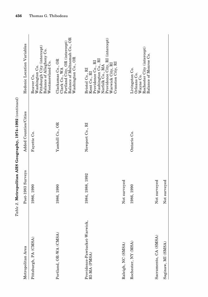
456 Thomas G. ThibodeauT
able
2.
Met
rop
oli
tan
AH
S G
eog
rap
hy
, 19
74–1
992
(con
tin
ued
)
Met
ropo
lita
n A
rea
Pos
t-19
83 S
urv
eys
Add
ed C
oun
ties
/Cit
ies
Hed
onic
Loc
atio
n V
aria
bles
Pit
tsbu
rgh
, P
A (
CM
SA
)19
86,
1990
Fay
ette
Co.
Bea
ver
Co.
Was
hin
gton
Co.
Pit
tsbu
rgh
Cit
y (i
nte
rcep
t)B
alan
ce o
f A
lleg
hen
y C
o.W
estm
orel
and
Co.
Por
tlan
d, O
R-W
A (
CM
SA
)19
86,
1990
Yam
hil
l C
o.,
OR
Cla
ckam
as C
o.,
OR
Cla
rk C
o.,
WA
Por
tlan
d C
ity,
OR
(in
terc
ept)
Bal
ance
of
Mu
ltn
omah
Co.
, O
RW
ash
ingt
on C
o.,
OR
Pr o
vide
nc e
-Paw
tuc k
et-W
arw
ick
,19
84,
1988
, 19
92N
ewpo
r t C
o.,
RI
Br i
stol
Co.
, R
IR
I-M
A (
PM
SA
)K
ent
Co.
, R
IP
r ovi
den
c e C
o.,
RI
Was
hin
gton
Co.
, R
IN
orfo
lk C
o.,
MA
Pro
vide
nce
Cit
y, R
I (i
nte
r cep
t)W
arw
ick
Cit
y, R
IC
r an
ston
Cit
y, R
I
Ral
eigh
, N
C (
SM
SA
)N
ot s
urv
eyed
Roc
hes
ter ,
NY
(M
SA
)19
86,
1990
On
tar i
o C
o.L
ivin
gsto
n C
o.O
r lea
ns
Co.
Way
ne
Co.
Roc
hes
ter
Cit
y (i
nte
r cep
t)B
alan
ce o
f M
onro
e C
o.
Sac
r am
ento
, C
A (
SM
SA
)N
ot s
urv
eyed
Sag
inaw
, M
I (S
MS
A)
Not
su
rvey
ed

House Price Indices from the 1984–1992 MSA American Housing Surveys 457T
able
2.
Met
rop
oli
tan
AH
S G
eog
rap
hy
, 19
74–1
992
(con
tin
ued
)
Met
ropo
lita
n A
rea
Pos
t-19
83 S
urv
eys
Add
ed C
oun
ties
/Cit
ies
Hed
onic
Loc
atio
n V
aria
bles
St.
Lou
is,
MO
-IL
(C
MS
A)
1987
, 19
91Je
rsey
Co.
, IL
Jeff
erso
n C
o.,
MO
Mon
roe
Co.
, IL
St.
Ch
arle
s C
o.,
MO
Cli
nto
n C
o.,
ILM
adis
on C
o.,
ILS
t. L
ouis
Cit
y, M
O (
inte
rcep
t)B
alan
ce o
f S
t. L
ouis
Co.
, M
OS
t. C
lair
Co.
, IL
Sal
t L
ake
Cit
y, U
T (
MS
A)
1984
, 19
88,
1992
Web
er C
o.S
alt
Lak
e C
ity
(in
terc
ept)
Bal
ance
of
Sal
t L
ake
Co.
Dav
is C
o.
San
An
ton
io,
TX
(M
SA
)19
86,
1990
Com
al C
o.S
an A
nto
nio
Cit
y (i
nte
r cep
t)B
alan
c e o
f B
exar
Co.
Gu
adal
upe
Co.
San
Ber
nar
din
o–R
iver
side
–19
86,
1990
Non
eS
an B
ern
ardi
no
Cit
yO
nta
r io,
CA
(P
MS
A)
Riv
ersi
de C
ity
(in
ter c
ept)
Bal
ance
of
Riv
ersi
de C
o.B
alan
ce o
f S
an B
ern
ardi
no
Co.
San
Die
go,
CA
(M
SA
)19
87,
1991
Non
eS
an D
iego
Cit
y (i
nte
r cep
t)B
alan
ce o
f S
an D
iego
Co.
San
Fra
nc i
sco–
Oak
lan
d, C
A19
85,
1989
Non
eS
an M
ateo
Co.
(PM
SA
)C
ontr
a C
osta
Co.
Mar
in C
o.S
an F
ran
c isc
o C
ity
(in
ter c
ept)
Oak
lan
d C
ity
Bal
ance
of
Ala
med
a C
o.
San
Jos
e, C
A (
adde
d in
198
4) (
MS
A)
1984
, 19
88S
an J
ose
Cit
y (i
nte
r cep
t)S
un
nyv
ale
Cit
yB
alan
ce o
f S
anta
Cla
ra C
o.

458 Thomas G. ThibodeauT
able
2.
Met
rop
oli
tan
AH
S G
eog
rap
hy
, 19
74–1
992
(con
tin
ued
)
Met
ropo
lita
n A
rea
Pos
t-19
83 S
urv
eys
Add
ed C
oun
ties
/Cit
ies
Hed
onic
Loc
atio
n V
aria
bles
Sea
ttle
-Eve
rett
, W
A (
CM
SA
)19
87,
1991
Par
t of
Sea
ttle
-S
noh
omis
h C
o.T
acom
a M
SA
Sea
ttle
Cit
y (i
nte
rcep
t)B
alan
ce o
f K
ing
Co.
Spo
kan
e, W
A (
SM
SA
)N
ot s
urv
eyed
Spr
ingf
ield
-Ch
icop
ee-H
olyo
ke,
MA
(S
MS
A)
Not
su
rvey
ed
Tac
oma,
WA
(M
SA
)19
87,
1991
Par
t of
Sea
ttle
-P
ierc
e C
o. (
inte
rcep
t)T
acom
a M
SA
Tam
pa–S
t. P
eter
sbu
rg,
FL
(ad
ded
in 1
985)
(M
SA
)19
85,
1989
Her
nan
do C
o.P
asco
Co.
Tam
pa C
ity
(in
ter c
ept)
St.
Pet
ersb
ur g
Cit
yB
alan
c e o
f P
inel
las
Co.
Bal
anc e
of
Hil
lsbo
r ou
gh C
o.
Was
hin
gton
, D
C-M
D-V
A (
MS
A)
1985
, 19
89F
rede
r ic k
Co.
, M
DM
ontg
omer
y C
o.,
MD
Sta
ffor
d C
o.,
VA
Ar l
ingt
on C
o.,
VA
Ch
arle
s C
o.,
MD
Lou
dou
n C
o.,
VA
Cal
ver t
Co.
, M
DW
ash
ingt
on,
DC
(in
ter c
ept)
Pr i
nc e
Geo
rge’
s C
o.,
MD
Fai
r fax
Co.
, V
A
Wic
hit
a, K
S (
SM
SA
)N
ot s
urv
eyed
Not
e : M
SA
= m
etr o
poli
tan
sta
tist
ical
ar e
a; C
MS
A =
con
soli
date
d m
etr o
poli
tan
sta
tist
ical
ar e
a; P
MS
A =
pr i
mar
y m
etr o
poli
tan
sta
tist
ical
ar e
a; S
MS
A =
stan
dard
met
r opo
lita
n s
tati
stic
al a
r ea.

House Price Indices from the 1984–1992 MSA American Housing Surveys 459
MSA house price indices are computed by pricing a constant bundle of housing charac-teristics using MSA estimated hedonic coefficients. Gillingham (1975); Goodman (1978);Follain and Malpezzi (1980); Linneman (1980); Malpezzi, Ozanne, and Thibodeau (1980);Thibodeau (1989, 1992); and others have used this procedure to measure the price ofhousing. Predicted values of the dependent variable in the transformed linear model areobtained by substituting estimated coefficients b and average housing characteristics X0
into equation (2) to yield
z
z NT T
0 0
0 02
01
0
=
( )( )−
X b
X X X X X
,
~ ,where � σ(6)
The constant-quality bundle that is priced is the average bundle of housing characteris-tics for all residential dwellings in large MSAs (census places with populations exceeding100,000). Average characteristics for the stock of urban housing are obtained from the1985 National AHS. The National AHS surveys about 70,000 residential dwellings inodd-numbered years.
House price indices are computed for the entire stock of housing within the metropolitanarea and for three quality-segmented submarkets: new housing, existing standard-quality housing, and substandard housing. For the entire-metropolitan-area house priceindex, average (tenure-specific) characteristics are computed for all residential dwellingslocated in large MSAs. Hence the housing characteristics that are priced represent theentire stock of housing in large urban areas rather than the characteristics peculiar toany one urban area. Average dwelling characteristics for substandard housing arecomputed using a definition of substandard housing formerly employed by HUD (1978).According to that definition, a residential dwelling is substandard if one or more of thefollowing conditions hold:
Plumbing. Unit lacks or shares complete plumbing (hot and cold running water,flush toilet, and bathtub or shower inside the structure).Kitchen. Unit lacks or shares a complete kitchen (installed sink with piped water,range or cook stove, and mechanical refrigerator).Sewage. Absence of a public sewer, septic tank, cesspool, or chemical toilet.Heating. There are no means of heating; or unit is heated by unvented room heatersburning gas, oil, or kerosene; or unit is heated by fireplace, stove, or portable roomheater (does not apply in South Census region).Maintenance. Unit suffers from any two of the following defects: leaking roof, opencracks or holes in interior walls or ceilings, holes in the interior floor, broken plasteror peeling paint (over one square foot) on interior walls or ceilings.Public hall. Unit suffers from any two of the following defects: public halls lacklight fixtures; loose, broken, or missing steps on common stairways; stair railingsloose or missing.Toilet access. Access to sole flush toilet is through one of two or more bedroomsused for sleeping (applies only to households with children under 18 years old).Electrical. Unit has exposed wiring, fuses blew or circuit breakers tripped three ormore times in the last 90 days, and unit lacks working outlet in one or more rooms.

460 Thomas G. Thibodeau
Average dwelling characteristics for new housing are computed for dwellings located inlarge MSAs that are less than three years old and not substandard according to thisdefinition. Existing standard-quality housing is defined to be housing that is neither newnor substandard.
The semilog hedonic specification introduces a statistical problem for computing houseprice indices. That is, the objective is to compute an unbiased estimator for either E{p0}or M{p0} rather than an unbiased estimator for the log of the house price. One potentialestimator, the “naive transformation,” takes the exponential of the predicted valueobtained from the semilog equation
p e ez0
0= = X b0 . (7)
Numerous authors (Aitchison and Brown 1957; Bradu and Mundlak 1970; Dhrymes1962; Finney 1941; Goldberger 1968; Haworth and Vincent 1979; Heien 1968; Meulenberg1965; Stynes, Peterson, and Rosenthal 1986; Teekens and Koerts 1972) have examinedthe statistical properties of the naive transformation and concluded that it is (1)asymptotically unbiased for the median of the house price distribution M{p0}, (2) biasedfor M{p0} in finite samples, and (3) asymptotically biased for the mean of the pricedistribution E{p0}. The bias introduced with the naive transformation can be substantial.Stynes, Peterson, and Rosenthal (1986) have demonstrated that the finite-sample bias inpublished studies on travel demand can be as high as 26 percent.
The finite sample unbiased estimator for median price in a semilog regression given byGoldberger (1968) is
p e F s T KM0
2 10 1
12
* ; , ,= − − − ( )
−X b X X X X0T T
0 (8)
where
F w v cf cw
jj
j
j
; ,!
,( ) =( )
=
∞
∑0
f
v vv jj
j
= ( ) ( )+( )
2 22�
�,
v T K= − ,
Γ t y e dy tt y( ) = >− −∞
∫ 1
00for ,
s
T K2 1
1=
− −ˆ ˆ ,u uT
T = the sample size,
K = the number of estimated parameters, and
û = the estimated residual.

House Price Indices from the 1984–1992 MSA American Housing Surveys 461
Finite-sample unbiased estimators for median house prices are computed using anapproximation to equation (8) (for details, see Thibodeau 1992). Correcting for the finite-sample bias is important even with the relatively large samples used here because thebias is a function of the residual variance, and the residual variance for the 1974–83hedonic equations increased systematically with the survey year.
Hedonic House Price Indices
MSA House Prices
MSA house price indices are listed in table 3 (for rental housing) and table 4 (for owner-occupied housing). The prices are listed alphabetically by metropolitan area beginningwith the places surveyed in 1984. Each table has six columns. The first two columns listthe MSA followed by the survey year. The last four columns list the house price indices.In table 3, PRMSA is the price of shelter rental housing services for the entire metropoli-tan area, PRNEW is the price of new rental housing services, PREXT is the price ofexisting standard-quality rental housing services, and PRSUB is the price of substan-dard rental housing services. The owner-occupied house price indices in table 4 aredefined similarly.
A year-by-year comparison of house prices indicates that New York City and Californiametropolitan areas consistently had the highest shelter rents. Shelter rents in thesehigh-priced housing markets were 1.9 to 3.2 times those in the least expensive housingmarkets. With some exceptions, the South (Birmingham, Houston, Oklahoma City, SanAntonio, and Tampa) had the markets with the lowest shelter rent. California MSAs(Anaheim, San Francisco, and San Jose) also had the highest priced owner-occupiedhousing. California MSA house prices were 2.9 to 4.6 times those in the least expensiveMSAs and 1.9 to 3.6 times the metropolitan average. Inexpensive owner-occupiedhousing was located throughout the South and the Midwest (Detroit, Houston, KansasCity, Memphis, Oklahoma City, St. Louis, and Tampa).
Measuring House Price Inflation
House price inflation is measured with three indices: a Laspeyres index, a Paasche index,and a Fisher index. The Laspeyres and Paasche indices are ratios of the ending-periodhousing expenditure to the beginning-period expenditure with expected expenditurescomputed using the bundle of housing characteristics from the beginning (Laspeyres) orending (Paasche) period. The Fisher index is simply the square root of the product of theLaspeyres and Paasche indices.
Both the Laspeyres and the Paasche indices price a constant bundle of housing charac-teristics over time. However, housing consumers modify their consumption patterns overtime in response to changes in price and in housing characteristics. An index is said tobe superlative if it accommodates changes in consumers’ expenditure patterns (Diewert1976). The Fisher index is superlative; the Laspeyres and Paasche indices are not.

462 Thomas G. ThibodeauT
able
3.
Mo
nth
ly P
rice
s o
f R
enta
l H
ou
sin
g S
erv
ices
PR
MS
AP
RN
EW
PR
EX
TP
RS
UB
MS
AS
urv
ey Y
ear
($)
($)
($)
($)
Bir
min
gham
, A
L19
8416
4.25
262.
4717
3.50
122.
83B
uff
alo,
NY
1984
208.
6328
3.88
217.
8016
7.16
Cle
vela
nd,
OH
1984
235.
5235
8.70
246.
5917
8.36
Indi
anap
olis
, IN
1984
186.
0731
4.69
195.
9713
8.85
Mem
phis
, T
N-A
R-M
S19
8417
9.99
305.
6019
1.06
130.
68M
ilw
auk
ee,
WI
1984
278.
5742
4.67
292.
8721
2.71
New
port
New
s–H
ampt
on,
VA
1984
225.
0331
7.69
233.
6218
3.19
Nor
folk
–Vir
gin
ia B
each
–New
port
New
s, V
A19
8423
6.90
337.
5124
9.06
176.
80O
kla
hom
a C
ity,
OK
1984
214.
6132
7.21
224.
4916
8.12
Pro
vide
nce
-Paw
tuck
et-W
arw
ick
, R
I-M
A19
8424
5.12
414.
6025
5.96
191.
34S
alt
Lak
e C
ity,
UT
1984
254.
8638
4.26
259.
8822
2.91
San
Jos
e, C
A19
8444
2.88
648.
1946
4.08
341.
32
Bos
ton
, M
A-N
H19
8536
3.01
456.
7537
8.67
292.
88D
alla
s, T
X19
8531
0.23
416.
3332
3.75
254.
77D
etr o
it,
MI
1985
281.
7545
3.30
293.
6921
6.65
For
t W
orth
, T
X19
8523
8.42
354.
5524
4.56
201.
91L
os A
nge
les–
Lon
g B
each
, C
A19
8541
4.95
580.
6343
1.73
336.
96M
inn
eapo
lis–
St.
Pau
l, M
N-W
I19
8532
5.87
435.
9933
4.76
276.
75P
hil
adel
phia
, P
A-N
J19
8530
0.22
450.
7231
4.45
234.
06P
hoe
nix
, A
Z19
8526
4.62
392.
7827
6.15
210.
56S
an F
ran
c isc
o–O
akla
nd,
CA
1985
431.
9062
5.82
447.
3335
4.57
Tam
pa–S
t. P
eter
sbu
rg,
FL
1985
210.
4931
1.97
220.
1616
5.29
Was
hin
gton
, D
C-M
D-V
A19
8537
3.63
533.
9938
3.36
314.
45
An
ahei
m–S
anta
An
a, C
A19
8650
9.22
672.
9751
4.23
470.
07C
inc i
nn
ati,
OH
-KY
-IN
1986
248.
1935
7.28
262.
3718
6.13
Den
ver ,
CO
1986
335.
0243
4.61
347.
2927
9.96
Kan
sas
Cit
y, M
O-K
S19
8622
6.01
386.
1323
8.26
169.
15M
iam
i–F
ort
Lau
derd
ale,
FL
1986
322.
1941
3.22
332.
2127
2.41
New
Or l
ean
s, L
A19
8625
3.75
311.
7926
2.55
218.
05P
itts
burg
h,
PA
1986
205.
7831
8.23
217.
5715
4.31
Por
tlan
d, O
R-W
A19
8628
7.69
439.
9529
9.94
227.
72R
och
este
r , N
Y19
8628
5.91
364.
0730
3.49
215.
83S
an A
nto
nio
, T
X19
8620
9.03
322.
1621
6.48
171.
84S
an B
ern
ardi
no–
Riv
ersi
de–O
nta
r io,
CA
1986
313.
2648
4.41
324.
0325
6.70
Atl
anta
, G
A19
8729
0.22
419.
6730
5.19
226.
45B
alti
mor
e, M
D19
8729
3.58
415.
3230
4.38
236.
63

House Price Indices from the 1984–1992 MSA American Housing Surveys 463T
able
3.
Mo
nth
ly P
rice
s o
f R
enta
l H
ou
sin
g S
erv
ices
(con
tin
ued
)
PR
MS
AP
RN
EW
PR
EX
TP
RS
UB
MS
AS
urv
ey Y
ear
($)
($)
($)
($)
Ch
icag
o, I
L19
8735
3.39
548.
9836
7.09
284.
46C
olu
mbu
s, O
H19
8724
9.65
402.
5326
0.33
194.
72H
artf
ord,
CT
1987
377.
0558
0.08
390.
1130
2.67
Hou
ston
, T
X19
8725
1.15
331.
8925
8.47
218.
98N
ew Y
ork
–Nas
sau
–Su
ffol
k,
NY
1987
498.
0771
7.52
517.
0840
6.40
New
ark
–Nor
thea
ster
n N
ew J
erse
y, N
J19
8742
0.11
750.
5044
1.92
313.
83P
ater
son
-Cli
fton
-Pas
saic
, N
J19
8745
7.10
656.
9547
9.85
354.
57S
t. L
ouis
, M
O-I
L19
8724
4.00
367.
3125
5.76
188.
15S
an D
iego
, C
A19
8742
7.99
576.
1343
8.46
372.
03S
eatt
le-E
vere
tt,
WA
1987
379.
7049
8.17
391.
6132
0.94
Tac
oma,
WA
1987
297.
9238
7.80
313.
2523
5.58
Bir
min
gham
, A
L19
8818
7.80
264.
5920
2.50
135.
14B
uff
alo,
NY
1988
267.
9837
4.98
277.
1222
1.70
Cle
vela
nd,
OH
1988
306.
7656
0.74
317.
8823
8.09
Indi
anap
olis
, IN
1988
246.
0338
7.41
256.
1319
1.57
Mem
phis
, T
N-A
R-M
S19
8824
3.55
376.
9725
5.27
187.
83M
ilw
auk
ee,
WI
1988
323.
1553
4.53
332.
0226
8.61
New
por t
New
s–H
ampt
on,
VA
1988
294.
1241
4.77
305.
5424
0.01
Nor
folk
–Vir
gin
ia B
each
–New
por t
New
s, V
A19
8829
8.27
413.
4930
7.37
244.
47O
kla
hom
a C
ity,
OK
1988
184.
0228
0.96
192.
6014
3.95
Pro
vide
nce
-Paw
tuck
et-W
arw
ick
, R
I-M
A19
8839
8.45
584.
7341
4.48
321.
17S
alt
Lak
e C
ity,
UT
1988
245.
5533
5.84
252.
8121
0.34
San
Jos
e, C
A19
8859
6.34
753.
1661
5.78
502.
92
Bos
ton
, M
A-N
H19
8955
7.44
701.
6358
8.26
432.
18D
alla
s, T
X19
8926
8.87
424.
0428
0.68
212.
10D
etr o
it,
MI
1989
344.
2854
3.62
353.
3427
4.48
For
t W
orth
, T
X19
8924
9.99
349.
9325
9.46
205.
14L
os A
nge
les–
Lon
g B
each
, C
A19
8954
8.42
691.
9156
9.89
453.
48M
inn
eapo
lis–
St.
Pau
l, M
N-W
I19
8936
4.24
466.
4738
2.13
287.
15P
hil
adel
phia
, P
A-N
J19
8939
0.39
576.
8440
2.34
322.
41P
hoe
nix
, A
Z19
8932
7.97
440.
3133
5.44
286.
21S
an F
ran
c isc
o–O
akla
nd,
CA
1989
572.
8571
2.46
589.
3249
8.24
Tam
pa–S
t. P
eter
sbu
rg,
FL
1989
234.
1037
8.16
237.
1621
6.04
Was
hin
gton
, D
C-M
D-V
A19
8948
4.07
631.
7350
0.56
402.
65

464 Thomas G. ThibodeauT
able
3.
Mo
nth
ly P
rice
s o
f R
enta
l H
ou
sin
g S
erv
ices
(co
nti
nu
ed)
PR
MS
AP
RN
EW
PR
EX
TP
RS
UB
MS
AS
urv
ey Y
ear
($)
($)
($)
($)
An
ahei
m–S
anta
An
a, C
A19
9066
4.64
823.
6467
9.68
586.
55C
inci
nn
ati,
OH
-KY
-IN
1990
281.
6137
7.27
290.
3923
7.42
Den
ver,
CO
1990
330.
2845
6.60
337.
3128
7.44
Kan
sas
Cit
y, M
O-K
S19
9027
3.88
410.
7528
8.11
208.
75M
iam
i–F
ort
Lau
derd
ale,
FL
1990
440.
5753
4.72
457.
9836
4.05
New
Orl
ean
s, L
A19
9027
9.78
370.
3728
7.38
244.
29P
itts
burg
h,
PA
1990
276.
6941
4.52
286.
5922
5.57
Por
tlan
d, O
R-W
A19
9035
1.20
541.
9736
6.91
274.
33R
och
este
r, N
Y19
9036
9.78
449.
7538
1.30
316.
05S
an A
nto
nio
, T
X19
9025
8.62
405.
9826
9.83
205.
11S
an B
ern
ardi
no–
Riv
ersi
de–O
nta
rio,
CA
1990
389.
9452
8.88
401.
5432
9.69
Atl
anta
, G
A19
9132
6.39
503.
8234
2.48
252.
71B
alti
mor
e, M
D19
9138
0.82
568.
9339
1.59
314.
34C
hic
ago,
IL
1991
436.
0470
1.39
461.
7532
4.47
Col
um
bus,
OH
1991
293.
4546
4.34
303.
4323
8.29
Har
tfor
d, C
T19
9148
5.07
649.
9750
7.51
379.
80H
oust
on,
TX
1991
284.
4338
3.94
296.
5323
1.46
New
Yor
k–N
assa
u–S
uff
olk
, N
Y19
9164
0.08
977.
4665
5.17
551.
79N
ewar
k–N
orth
east
ern
New
Jer
sey,
NJ
1991
514.
1745
7.29
527.
9446
1.45
Pat
erso
n-C
lift
on-P
assa
ic,
NJ
1991
505.
3782
9.54
524.
0939
9.30
St.
Lou
is,
MO
-IL
1991
297.
1742
9.91
304.
3524
9.93
San
Die
go,
CA
1991
605.
1765
8.36
624.
3352
6.61
Sea
ttle
-Eve
rett
, W
A19
9147
4.51
618.
3949
4.76
385.
88T
acom
a, W
A19
9138
0.08
648.
4039
3.37
306.
59
Bir
min
gham
, A
L19
9221
5.82
350.
6922
6.70
163.
46C
leve
lan
d, O
H19
9232
5.60
472.
1334
2.83
241.
90In
dian
apol
is,
IN19
9230
1.63
447.
7231
2.41
246.
98M
emph
is,
TN
-AR
-MS
1992
249.
4341
6.72
263.
4118
5.49
New
por t
New
s–H
ampt
on,
VA
1992
342.
2446
2.32
358.
7027
0.70
Nor
folk
–Vir
gin
ia B
each
–New
por t
New
s, V
A19
9232
1.74
443.
3033
2.75
264.
04O
kla
hom
a C
ity,
OK
1992
221.
9432
6.18
231.
1117
8.27
Pro
vide
nce
-Paw
tuck
et-W
arw
ick
, R
I-M
A19
9241
6.88
595.
5743
2.06
341.
97S
alt
Lak
e C
ity,
UT
1992
319.
7845
2.79
328.
9027
1.11

House Price Indices from the 1984–1992 MSA American Housing Surveys 465T
able
4.
Pri
ces
of
Ow
ner
-Occ
up
ied
Ho
usi
ng
PO
MS
AP
ON
EW
PO
EX
TP
OS
UB
MS
AS
urv
ey Y
ear
($)
($)
($)
($)
Bir
min
gham
, A
L19
8444
,667
73,4
0146
,066
30,0
53B
uff
alo,
NY
1984
43,4
7984
,629
44,0
7933
,345
Cle
vela
nd,
OH
1984
56,4
7399
,730
57,0
1346
,344
Indi
anap
olis
, IN
1984
44,3
2578
,585
44,7
1336
,421
Mem
phis
, T
N-A
R-M
S19
8443
,345
85,9
8344
,175
31,4
48M
ilw
auk
ee,
WI
1984
60,1
2910
7,34
560
,964
46,2
78N
ewpo
rt N
ews–
Ham
pton
, V
A19
8453
,957
82,0
1454
,588
43,5
95N
orfo
lk–V
irgi
nia
Bea
ch–N
ewpo
rt N
ews,
VA
1984
58,5
2886
,629
59,3
3845
,148
Ok
lah
oma
Cit
y, O
K19
8455
,666
97,0
8856
,553
43,5
30P
rovi
den
ce-P
awtu
cket
-War
wic
k,
RI-
MA
1984
62,1
1111
2,62
662
,328
53,0
81S
alt
Lak
e C
ity,
UT
1984
64,3
9792
,959
64,9
1355
,821
San
Jos
e, C
A19
8414
3,29
016
0,54
714
4,49
313
3,13
4
Bos
ton
, M
A-N
H19
8511
3,61
316
2,32
611
4,58
697
,764
Dal
las,
TX
1985
77,2
9411
9,12
879
,987
52,2
72D
etr o
it,
MI
1985
43,4
6386
,496
44,1
3932
,667
For
t W
orth
, T
X19
8554
,238
103,
878
55,0
2941
,154
Los
An
gele
s–L
ong
Bea
ch,
CA
1985
131,
516
175,
194
133,
452
108,
084
Min
nea
poli
s–S
t. P
aul,
MN
-WI
1985
66,1
1010
6,36
765
,978
60,5
13P
hil
adel
phia
, P
A-N
J19
8557
,246
96,7
7458
,287
43,3
33P
hoe
nix
, A
Z19
8572
,764
119,
925
73,2
4661
,477
San
Fra
nc i
sco–
Oak
lan
d, C
A19
8513
6,89
416
9,91
113
9,46
111
0,13
7T
ampa
–St.
Pet
ersb
urg
, F
L19
8548
,169
86,0
1848
,656
40,1
95W
ash
ingt
on,
DC
-MD
-VA
1985
92,4
5512
2,11
093
,576
78,4
35
An
ahei
m–S
anta
An
a, C
A19
8614
2,50
119
8,28
614
2,86
512
8,99
2C
inc i
nn
ati,
OH
-KY
-IN
1986
52,0
1083
,705
52,5
4942
,613
Den
ver ,
CO
1986
80,8
4313
1,43
080
,908
73,4
62K
ansa
s C
ity,
MO
-KS
1986
45,1
3990
,225
46,0
2131
,807
Mia
mi–
For
t L
aude
rdal
e, F
L19
8681
,140
123,
200
81,2
7174
,790
New
Or l
ean
s, L
A19
8666
,740
98,0
1668
,300
50,0
98P
itts
burg
h,
PA
1986
48,6
6311
2,88
848
,924
38,8
76P
ortl
and,
OR
-WA
1986
64,7
6310
3,56
065
,068
55,6
19R
och
este
r , N
Y19
8667
,393
112,
661
68,4
3851
,353
San
An
ton
io,
TX
1986
61,8
1210
5,45
763
,139
44,9
02S
an B
ern
ardi
no–
Riv
ersi
de–O
nta
r io,
CA
1986
90,2
0812
6,11
691
,442
73,6
35

466 Thomas G. ThibodeauT
able
4. P
rice
s o
f O
wn
er-O
ccu
pie
d H
ou
sin
g (c
onti
nu
ed)
PO
MS
AP
ON
EW
PO
EX
TP
OS
UB
MS
AS
urv
ey Y
ear
($)
($)
($)
($)
Atl
anta
, G
A19
8772
,049
104,
106
72,8
4963
,697
Bal
tim
ore,
MD
1987
77,1
8914
1,96
777
,167
65,4
42C
hic
ago,
IL
1987
81,1
7012
5,11
581
,989
67,2
53C
olu
mbu
s, O
H19
8758
,210
89,3
5558
,516
50,3
43H
artf
ord,
CT
1987
135,
427
217,
181
136,
782
111,
657
Hou
ston
, T
X19
8757
,624
79,7
9659
,071
42,8
19N
ew Y
ork
–Nas
sau
–Su
ffol
k,
NY
1987
158,
675
251,
603
162,
473
115,
945
New
ark
–Nor
thea
ster
n N
ew J
erse
y, N
J19
8715
6,58
123
6,38
215
7,38
613
4,02
0P
ater
son
-Cli
fton
-Pas
saic
, N
J19
8717
6,16
429
2,33
117
5,69
416
5,74
2S
t. L
ouis
, M
O-I
L19
8752
,204
95,8
0053
,109
38,6
50S
an D
iego
, C
A19
8713
4,16
318
0,11
513
5,91
211
2,18
9S
eatt
le-E
vere
tt,
WA
1987
82,2
7911
8,88
083
,045
72,2
16T
acom
a, W
A19
8779
,169
130,
624
80,9
9057
,406
Bir
min
gham
, A
L19
8850
,310
86,8
2851
,685
35,6
78B
uff
alo,
NY
1988
53,1
1210
0,14
353
,626
42,3
07C
leve
lan
d, O
H19
8856
,166
102,
478
56,8
8743
,236
Indi
anap
olis
, IN
1988
50,3
4198
,339
51,2
4737
,122
Mem
phis
, T
N-A
R-M
S19
8859
,083
107,
989
60,5
3040
,708
Mil
wau
kee
, W
I19
8858
,675
103,
548
59,6
2444
,312
New
por t
New
s–H
ampt
on,
VA
1988
80,7
5611
6,35
382
,275
62,2
03N
orfo
lk–V
irgi
nia
Bea
ch–N
ewpo
r t N
ews,
VA
1988
77,3
4211
0,00
178
,682
61,2
95O
kla
hom
a C
ity,
OK
1988
45,8
4176
,304
46,6
5335
,176
Pro
vide
nce
-Paw
tuck
et-W
arw
ick
, R
I-M
A19
8814
1,11
023
4,53
814
1,10
612
7,89
2S
alt
Lak
e C
ity,
UT
1988
62,9
0410
3,19
763
,319
53,7
14S
an J
ose,
CA
1988
211,
582
263,
894
214,
099
187,
439
Bos
ton
, M
A-N
H19
8917
4,26
823
8,21
417
5,60
915
1,64
8D
alla
s, T
X19
8969
,434
110,
759
71,1
7451
,990
Det
r oit
, M
I19
8957
,845
137,
077
58,6
7740
,940
For
t W
orth
, T
X19
8960
,561
102,
536
61,9
9543
,515
Los
An
gele
s–L
ong
Bea
ch,
CA
1989
207,
351
220,
612
213,
346
156,
258
Min
nea
poli
s–S
t. P
aul,
MN
-WI
1989
75,2
7512
4,39
176
,103
61,3
05P
hil
adel
phia
, P
A-N
J19
8993
,762
172,
880
96,1
1264
,089
Ph
oen
ix,
AZ
1989
68,5
7911
8,08
469
,743
52,9
08S
an F
ran
c isc
o–O
akla
nd,
CA
1989
224,
781
258,
013
231,
536
170,
610
Tam
pa–S
t. P
eter
sbu
rg,
FL
1989
56,9
8811
5,71
156
,720
52,3
25W
ash
ingt
on,
DC
-MD
-VA
1989
135,
301
178,
794
136,
182
120,
912

House Price Indices from the 1984–1992 MSA American Housing Surveys 467T
able
4. P
rice
s o
f O
wn
er-O
ccu
pie
d H
ou
sin
g (c
onti
nu
ed)
PO
MS
AP
ON
EW
PO
EX
TP
OS
UB
MS
AS
urv
ey Y
ear
($)
($)
($)
($)
An
ahei
m–S
anta
An
a, C
A19
9015
5,02
022
9,16
114
9,00
920
6,89
7C
inci
nn
ati,
OH
-KY
-IN
1990
62,5
1811
3,81
662
,796
52,9
29D
enve
r, C
O19
9078
,794
133,
657
78,9
7770
,170
Kan
sas
Cit
y, M
O-K
S19
9048
,243
100,
013
48,8
6536
,141
Mia
mi–
For
t L
aude
rdal
e, F
L19
9089
,242
132,
546
90,7
7871
,756
New
Orl
ean
s, L
A19
9068
,452
94,8
1170
,208
50,9
67P
itts
burg
h,
PA
1990
53,3
6311
0,37
154
,552
37,0
08P
ortl
and,
OR
-WA
1990
71,6
3512
6,20
171
,684
62,5
39R
och
este
r, N
Y19
9082
,938
136,
856
83,4
6168
,539
San
An
ton
io,
TX
1990
61,0
2210
2,77
262
,317
44,5
21S
an B
ern
ardi
no–
Riv
ersi
de–O
nta
rio,
CA
1990
125,
319
167,
221
125,
529
112,
032
Atl
anta
, G
A19
9177
,031
113,
590
78,6
0558
,777
Bal
tim
ore,
MD
1991
95,8
1815
5,03
394
,963
88,2
21C
hic
ago,
IL
1991
88,6
0114
0,06
190
,698
63,6
73C
olu
mbu
s, O
H19
9161
,263
96,8
7861
,463
54,0
69H
artf
ord,
CT
1991
150,
049
202,
296
150,
346
138,
590
Hou
ston
, T
X19
9154
,826
86,8
1961
,816
40,1
78N
ew Y
ork
–Nas
sau
–Su
ffol
k,
NY
1991
167,
310
269,
153
169,
119
135,
999
New
ark
–Nor
thea
ster
n N
ew J
erse
y, N
J19
9114
6,58
222
2,61
614
7,57
912
3,86
6P
ater
son
-Cli
fton
-Pas
saic
, N
J19
9119
8,12
838
5,91
019
8,33
015
5,39
7S
t. L
ouis
, M
O-I
L19
9154
,917
95,7
5155
,844
40,1
32S
an D
iego
, C
A19
9120
3,53
725
6,66
720
7,10
416
4,76
6S
eatt
le-E
vere
tt,
WA
1991
150,
078
214,
748
152,
458
120,
981
Tac
oma,
WA
1991
94,1
2316
4,14
495
,261
75,1
71
Bir
min
gham
, A
L19
9255
,399
100,
880
56,8
5838
,323
Cle
vela
nd,
OH
1992
74,5
8113
4,56
175
,205
60,8
49In
dian
apol
is,
IN19
9262
,020
118,
323
62,4
6550
,960
Mem
phis
, T
N-A
R-M
S19
9264
,817
117,
360
66,0
4646
,796
New
por t
New
s–H
ampt
on,
VA
1992
85,9
6612
1,65
487
,919
63,7
28N
orfo
lk–V
irgi
nia
Bea
ch–N
ewpo
r t N
ews,
VA
1992
81,2
1412
1,68
982
,162
66,2
37O
kla
hom
a C
ity,
OK
1992
45,7
8488
,631
46,7
8332
,762
Pro
vide
nce
-Paw
tuck
et-W
arw
ick
, R
I-M
A19
9213
0,81
619
4,65
113
2,58
710
5,50
0S
alt
Lak
e C
ity,
UT
1992
70,2
0911
8,25
670
,882
57,5
44
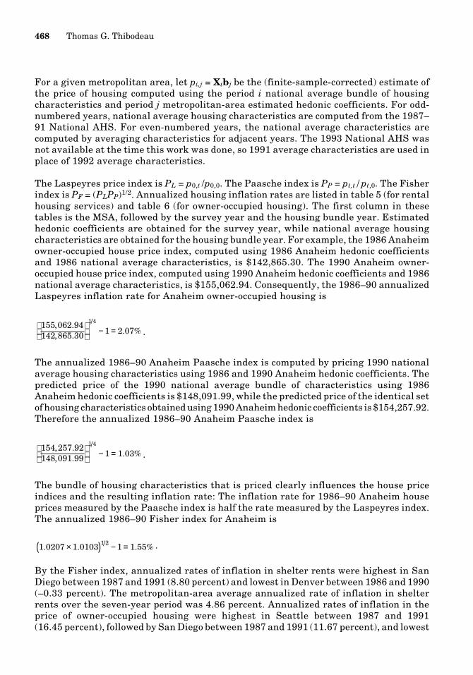
468 Thomas G. Thibodeau
For a given metropolitan area, let pi,j = Xibj be the (finite-sample-corrected) estimate ofthe price of housing computed using the period i national average bundle of housingcharacteristics and period j metropolitan-area estimated hedonic coefficients. For odd-numbered years, national average housing characteristics are computed from the 1987–91 National AHS. For even-numbered years, the national average characteristics arecomputed by averaging characteristics for adjacent years. The 1993 National AHS wasnot available at the time this work was done, so 1991 average characteristics are used inplace of 1992 average characteristics.
The Laspeyres price index is PL = p0,t /p0,0. The Paasche index is PP = pt,t/pt,0. The Fisherindex is PF = (PLPP)1/2. Annualized housing inflation rates are listed in table 5 (for rentalhousing services) and table 6 (for owner-occupied housing). The first column in thesetables is the MSA, followed by the survey year and the housing bundle year. Estimatedhedonic coefficients are obtained for the survey year, while national average housingcharacteristics are obtained for the housing bundle year. For example, the 1986 Anaheimowner-occupied house price index, computed using 1986 Anaheim hedonic coefficientsand 1986 national average characteristics, is $142,865.30. The 1990 Anaheim owner-occupied house price index, computed using 1990 Anaheim hedonic coefficients and 1986national average characteristics, is $155,062.94. Consequently, the 1986–90 annualizedLaspeyres inflation rate for Anaheim owner-occupied housing is
155 062 94142 865 30 1 2 07
1 4, ., . . %
− = .
The annualized 1986–90 Anaheim Paasche index is computed by pricing 1990 nationalaverage housing characteristics using 1986 and 1990 Anaheim hedonic coefficients. Thepredicted price of the 1990 national average bundle of characteristics using 1986Anaheim hedonic coefficients is $148,091.99, while the predicted price of the identical setof housing characteristics obtained using 1990 Anaheim hedonic coefficients is $154,257.92.Therefore the annualized 1986–90 Anaheim Paasche index is
154 257 92148 091 99 1 1 03
1 4, ., . . %
− = .
The bundle of housing characteristics that is priced clearly influences the house priceindices and the resulting inflation rate: The inflation rate for 1986–90 Anaheim houseprices measured by the Paasche index is half the rate measured by the Laspeyres index.The annualized 1986–90 Fisher index for Anaheim is
1 0207 1 0103 1 1 551 2. . . %×( ) − = .
By the Fisher index, annualized rates of inflation in shelter rents were highest in SanDiego between 1987 and 1991 (8.80 percent) and lowest in Denver between 1986 and 1990(–0.33 percent). The metropolitan-area average annualized rate of inflation in shelterrents over the seven-year period was 4.86 percent. Annualized rates of inflation in theprice of owner-occupied housing were highest in Seattle between 1987 and 1991(16.45 percent), followed by San Diego between 1987 and 1991 (11.67 percent), and lowest

House Price Indices from the 1984–1992 MSA American Housing Surveys 469T
able
5. I
nfl
ati
on
Ra
tes
for
Ren
tal
Ho
usi
ng
Ser
vic
es
Hou
sin
gH
ouse
An
nu
alL
aspe
yres
Paa
sch
eF
ish
erS
urv
eyB
un
dle
Pri
ceC
han
ge i
n Q
Infl
atio
nIn
flat
ion
Infl
atio
nM
SA
Yea
rY
ear
($)
(%)
Rat
e (%
)R
ate
(%)
Rat
e (%
)
An
ahei
m–S
anta
An
a, C
A19
8619
8650
5.41
1986
1990
503.
68–0
.09
1990
1986
664.
037.
0619
9019
9067
1.26
0.27
7.44
7.25
Atl
anta
, G
A19
8719
8729
2.44
1987
1991
297.
660.
4419
9119
8732
9.71
3.04
1991
1991
336.
020.
483.
083.
06B
alti
mor
e, M
D19
8719
8729
3.70
1987
1991
294.
410.
0619
9119
8738
2.71
6.84
1991
1991
383.
560.
066.
846.
84B
irm
ingh
am,
AL
1988
1988
188.
6019
8819
9118
9.03
0.08
1992
1988
217.
643.
6519
9219
9121
8.14
0.08
3.65
3.65
Ch
icag
o, I
L19
8719
8735
6.32
1987
1991
363.
850.
5219
9119
8743
6.96
5.23
1991
1991
438.
960.
114.
805.
02C
inc i
nn
ati,
OH
-KY
-IN
1986
1986
250.
0519
8619
9025
5.77
0.57
1990
1986
282.
543.
1019
9019
9028
8.23
0.50
3.03
3.07
Cle
vela
nd,
OH
1988
1988
307.
1319
8819
9130
7.42
0.03
1992
1988
332.
762.
0219
9219
9133
7.94
0.52
2.39
2.21
Col
um
bus,
OH
1987
1987
251.
2819
8719
9125
5.10
0.38
1991
1987
296.
174.
1919
9119
9130
2.42
0.52
4.35
4.27
Den
ver ,
CO
1986
1986
335.
0319
8619
9033
5.00
0.00
1990
1986
329.
57–0
.41
1990
1990
331.
730.
16–0
. 24
–0. 3
3
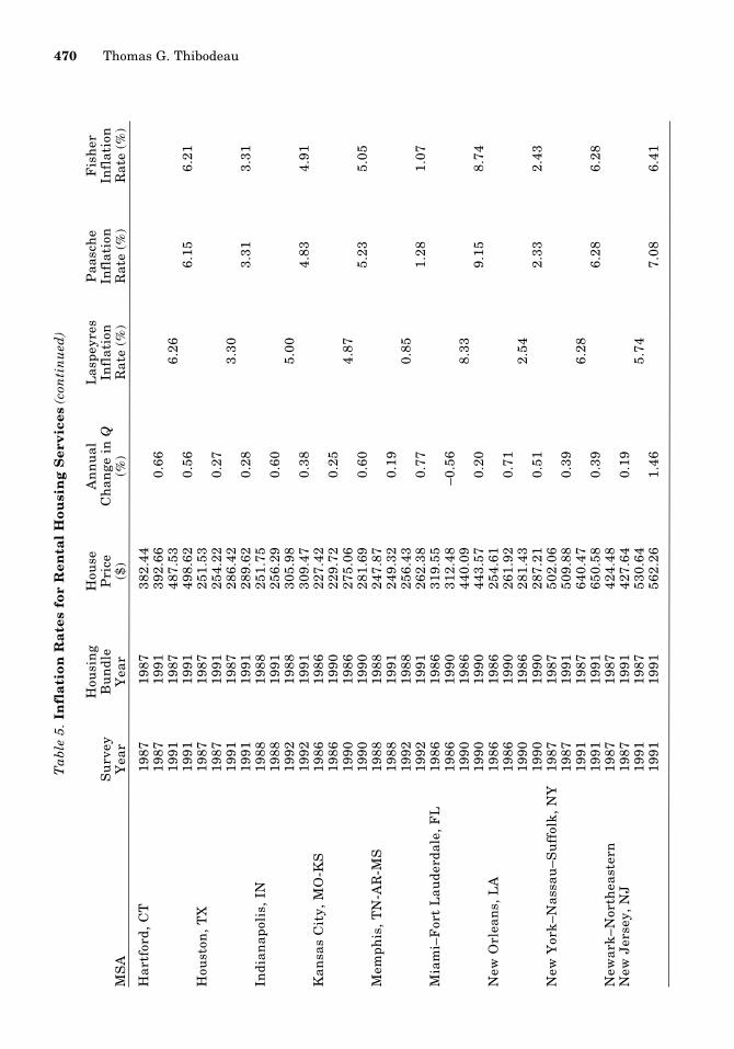
470 Thomas G. ThibodeauT
able
5. I
nfl
ati
on
Ra
tes
for
Ren
tal
Ho
usi
ng
Ser
vic
es (c
onti
nu
ed)
Hou
sin
gH
ouse
An
nu
alL
aspe
yres
Paa
sch
eF
ish
erS
urv
eyB
un
dle
Pri
ceC
han
ge i
n Q
Infl
atio
nIn
flat
ion
Infl
atio
nM
SA
Yea
rY
ear
($)
(%)
Rat
e (%
)R
ate
(%)
Rat
e (%
)
Har
tfor
d, C
T19
8719
8738
2.44
1987
1991
392.
660.
6619
9119
8748
7.53
6.26
1991
1991
498.
620.
566.
156.
21H
oust
on,
TX
1987
1987
251.
5319
8719
9125
4.22
0.27
1991
1987
286.
423.
3019
9119
9128
9.62
0.28
3.31
3.31
Indi
anap
olis
, IN
1988
1988
251.
7519
8819
9125
6.29
0.60
1992
1988
305.
985.
0019
9219
9130
9.47
0.38
4.83
4.91
Kan
sas
Cit
y, M
O-K
S19
8619
8622
7.42
1986
1990
229.
720.
2519
9019
8627
5.06
4.87
1990
1990
281.
690.
605.
235.
05M
emph
is,
TN
-AR
-MS
1988
1988
247.
8719
8819
9124
9.32
0.19
1992
1988
256.
430.
8519
9219
9126
2.38
0.77
1.28
1.07
Mia
mi–
For
t L
aude
rdal
e, F
L19
8619
8631
9.55
1986
1990
312.
48–0
.56
1990
1986
440.
098.
3319
9019
9044
3.57
0.20
9.15
8.74
New
Or l
ean
s, L
A19
8619
8625
4.61
1986
1990
261.
920.
7119
9019
8628
1.43
2.54
1990
1990
287.
210.
512.
332.
43N
ew Y
ork
–Nas
sau
–Su
ffol
k,
NY
1987
1987
502.
0619
8719
9150
9.88
0.39
1991
1987
640.
476.
2819
9119
9165
0.58
0.39
6.28
6.28
New
ark
–Nor
thea
ster
n19
8719
8742
4.48
New
Jer
sey,
NJ
1987
1991
427.
640.
1919
9119
8753
0.64
5.74
1991
1991
562.
261.
467.
086.
41

House Price Indices from the 1984–1992 MSA American Housing Surveys 471T
able
5. I
nfl
ati
on
Ra
tes
for
Ren
tal
Ho
usi
ng
Ser
vic
es (c
onti
nu
ed)
Hou
sin
gH
ouse
An
nu
alL
aspe
yres
Paa
sch
eF
ish
erS
urv
eyB
un
dle
Pri
ceC
han
ge i
n Q
Infl
atio
nIn
flat
ion
Infl
atio
nM
SA
Yea
rY
ear
($)
(%)
Rat
e (%
)R
ate
(%)
Rat
e (%
)
New
port
New
s–H
ampt
on,
VA
1988
1988
289.
9419
8819
9127
9.69
–1.1
919
9219
8834
2.20
4.23
1992
1991
340.
80–0
.14
5.06
4.65
Nor
folk
–Vir
gin
ia B
each
–19
8819
8830
0.67
New
port
New
s, V
A19
8819
9130
0.38
–0.0
319
9219
8832
2.34
1.76
1992
1991
318.
76–0
.37
1.50
1.63
Ok
lah
oma
Cit
y, O
K19
8819
8818
3.90
1988
1991
182.
61–0
.23
1992
1988
224.
875.
1619
9219
9122
6.28
0.21
5.51
5.33
Pat
erso
n-C
lift
on-P
assa
ic,
NJ
1987
1987
450.
5619
8719
9144
2.91
–0.4
319
9119
8750
9.03
3.10
1991
1991
518.
080.
444.
003.
55P
itts
burg
h,
PA
1986
1986
205.
3219
8619
9020
3.36
–0.2
419
9019
8627
7.77
7.85
1990
1990
283.
780.
548.
698.
27P
ortl
and,
OR
-WA
1986
1986
288.
6019
8619
9029
0.24
0.14
1990
1986
351.
875.
0819
9019
9035
7.52
0.40
5.35
5.22
Pro
vide
nce
-Paw
tuck
et-
1988
1988
401.
38W
arw
ick
, R
I-M
A19
8819
9140
4.11
0.23
1992
1988
425.
371.
4619
9219
9143
2.93
0.59
1.74
1.60
Roc
hes
ter ,
NY
1986
1986
288.
5219
8619
9029
9.68
0.95
1990
1986
372.
266.
5819
9019
9038
4.21
0.79
6.41
6.49

472 Thomas G. ThibodeauT
able
5. I
nfl
ati
on
Ra
tes
for
Ren
tal
Ho
usi
ng
Ser
vic
es (c
onti
nu
ed)
Hou
sin
gH
ouse
An
nu
alL
aspe
yres
Paa
sch
eF
ish
erS
urv
eyB
un
dle
Pri
ceC
han
ge i
n Q
Infl
atio
nIn
flat
ion
Infl
atio
nM
SA
Yea
rY
ear
($)
(%)
Rat
e (%
)R
ate
(%)
Rat
e (%
)
St.
Lou
is,
MO
-IL
1987
1987
243.
5319
8719
9124
2.17
–0.1
419
9119
8729
7.62
5.14
1991
1991
300.
660.
255.
565.
35S
alt
Lak
e C
ity,
UT
1988
1988
248.
2619
8819
9125
0.84
0.35
1992
1988
319.
926.
5519
9219
9131
9.98
0.01
6.28
6.41
San
An
ton
io,
TX
1986
1986
207.
6119
8619
9020
6.44
–0.1
419
9019
8625
8.04
5.59
1990
1990
257.
64–0
.04
5.70
5.64
San
Ber
nar
din
o–R
iver
side
–19
8619
8631
3.77
On
tar i
o, C
A19
8619
9031
9.34
0.44
1990
1986
393.
495.
8219
9019
9040
7.60
0.88
6.29
6.06
San
Die
go,
CA
1987
1987
427.
2319
8719
9143
0.78
0.21
1991
1987
607.
189.
1919
9119
9159
5.12
–0.5
08.
418.
80S
eatt
le–E
vere
tt,
WA
1987
1987
377.
2319
8719
9137
5.20
–0.1
319
9119
8747
4.06
5.88
1991
1991
479.
530.
296.
336.
10T
acom
a, W
A19
8719
8730
0.30
1987
1991
308.
670.
6919
9119
8738
2.17
6.21
1991
1991
383.
190.
075.
565.
88A
vera
ge0.
254.
774.
954.
86

House Price Indices from the 1984–1992 MSA American Housing Surveys 473T
able
6.
Infl
ati
on
Ra
tes
for
Ow
ner
-Occ
up
ied
Ho
usi
ng
Hou
sin
gH
ouse
An
nu
alL
aspe
yres
Paa
sch
eF
ish
erS
urv
eyB
un
dle
Pri
ceC
han
ge i
n Q
Infl
atio
nIn
flat
ion
Infl
atio
nM
SA
Yea
rY
ear
($)
(%)
Rat
e (%
)R
ate
(%)
Rat
e (%
)
An
ahei
m–S
anta
An
a, C
A19
8619
8614
2,86
5.30
1986
1990
148,
091.
990.
9019
9019
8615
5,06
2.94
2.07
1990
1990
154,
257.
92–0
.13
1.03
1.55
Atl
anta
, G
A19
8719
8772
,067
.41
1987
1991
72,8
33.0
70.
2619
9119
8777
,051
.83
1.69
1991
1991
78,2
46.7
30.
391.
811.
75B
alti
mor
e, M
D19
8719
8779
,203
.00
1987
1991
80,6
75.6
20.
4619
9119
8796
,989
.79
5.20
1991
1991
99,1
19.6
00.
545.
285.
24B
irm
ingh
am,
AL
1988
1988
50,8
82.1
919
8819
9150
,552
.87
–0.2
219
9219
8856
,254
.47
2.54
1992
1991
56,7
85.8
30.
312.
952.
74C
hic
ago,
IL
1987
1987
81,4
74.5
319
8719
9182
,657
.01
0.36
1991
1987
89,8
25.2
82.
4719
9119
9193
,289
.43
0.95
3.07
2.77
Cin
c in
nat
i, O
H-K
Y-I
N19
8619
8651
,828
.60
1986
1990
51,9
56.0
20.
0619
9019
8662
,447
.79
4.77
1990
1990
63,4
76.1
30.
415.
134.
95C
leve
lan
d, O
H19
8819
8856
,896
.67
1988
1991
57,1
80.4
40.
1719
9219
8874
,095
.36
6.83
1992
1991
74,1
79.1
60.
046.
726.
77C
olu
mbu
s, O
H19
8719
8758
,518
.14
1987
1991
59,0
70.2
00.
2419
9119
8761
,140
.07
1.10
1991
1991
64,0
50.6
11.
172.
041.
57D
enve
r , C
O19
8619
8681
,090
.12
1986
1990
82,6
54.5
70.
4819
9019
8677
,968
.63
–0.9
819
9019
9076
, 471
. 07
–0. 4
8–1
. 93
–1. 4
5

474 Thomas G. ThibodeauT
able
6.
Infl
ati
on
Ra
tes
for
Ow
ner
-Occ
up
ied
Ho
usi
ng
(co
nti
nu
ed)
Hou
sin
gH
ouse
An
nu
alL
aspe
yres
Paa
sch
eF
ish
erS
urv
eyB
un
dle
Pri
ceC
han
ge i
n Q
Infl
atio
nIn
flat
ion
Infl
atio
nM
SA
Yea
rY
ear
($)
(%)
Rat
e (%
)R
ate
(%)
Rat
e (%
)
Har
tfor
d, C
T19
8719
8713
7,99
3.91
1987
1991
143,
156.
830.
9219
9119
8715
1,49
8.36
2.36
1991
1991
154,
190.
900.
441.
872.
12H
oust
on,
TX
1987
1987
58,8
71.5
519
8719
9163
,515
.86
1.92
1991
1987
54,5
58.3
1–1
.88
1991
1991
56,5
28.2
40.
89–2
.87
–2.3
8In
dian
apol
is,
IN19
8819
8850
,922
.21
1988
1991
51,0
55.3
90.
0919
9219
8862
,614
.27
5.30
1992
1991
62,8
76.5
10.
145.
345.
32K
ansa
s C
ity,
MO
-KS
1986
1986
45,6
45.1
719
8619
9047
,988
.87
1.26
1990
1986
48,7
17.3
11.
6419
9019
9050
,571
.15
0.94
1.32
1.48
Mem
phis
, T
N-A
R-M
S19
8819
8859
,913
.71
1988
1991
60,5
45.4
90.
3519
9219
8866
,460
.34
2.63
1992
1991
68,6
58.5
71.
093.
192.
91M
iam
i–F
ort
Lau
derd
ale,
FL
1986
1986
80,9
75.6
719
8619
9083
,465
.21
0.76
1990
1986
89,3
30.8
32.
4919
9019
9093
,342
.51
1.10
2.84
2.66
New
Or l
ean
s, L
A19
8619
8667
,214
.53
1986
1990
70,6
17.4
81.
2419
9019
8668
,536
.60
0.49
1990
1990
70,7
40.3
10.
790.
040.
27N
ew Y
ork
–Nas
sau
–19
8719
8716
1,57
0.96
Su
ffol
k,
NY
1987
1991
168,
257.
821.
0219
9119
8717
0,71
3.88
1.39
1991
1991
178,
635.
781.
141.
511.
45N
ewar
k–N
orth
east
ern
1987
1987
161,
066.
55N
ew J
erse
y, N
J19
8719
9115
9,80
4.80
–0.2
019
9119
8714
8,99
6.25
–1.9
319
9119
9114
9,41
9.52
0.07
–1.6
7–1
.80

House Price Indices from the 1984–1992 MSA American Housing Surveys 475T
able
6.
Infl
ati
on
Ra
tes
for
Ow
ner
-Occ
up
ied
Ho
usi
ng
(co
nti
nu
ed)
Hou
sin
gH
ouse
An
nu
alL
aspe
yres
Paa
sch
eF
ish
erS
urv
eyB
un
dle
Pri
ceC
han
ge i
n Q
Infl
atio
nIn
flat
ion
Infl
atio
nM
SA
Yea
rY
ear
($)
(%)
Rat
e (%
)R
ate
(%)
Rat
e (%
)
New
port
New
s–H
ampt
on,
VA
1988
1988
79,2
33.7
019
8819
9177
,763
.34
–0.6
219
9219
8883
,351
.44
1.27
1992
1991
81,3
74.3
1–0
.80
1.14
1.21
Nor
folk
–Vir
gin
ia B
each
–19
8819
8876
,553
.39
New
port
New
s, V
A19
8819
9175
,797
.30
–0.3
319
9219
8881
,397
.39
1.55
1992
1991
81,9
45.6
00.
221.
971.
76O
kla
hom
a C
ity,
OK
1988
1988
46,9
21.5
219
8819
9148
,290
.43
0.96
1992
1988
46,1
50.3
3–0
.41
1992
1991
47,2
78.8
80.
81–0
.53
–0.4
7P
ater
son
-Cli
fton
-Pas
saic
, N
J19
8719
8717
4,97
5.65
1987
1991
182,
165.
961.
0119
9119
8719
8,21
2.08
3.17
1991
1991
201,
566.
200.
422.
562.
86P
itts
burg
h,
PA
1986
1986
48,5
63.2
719
8619
9048
,758
.74
0.10
1990
1986
53,3
95.3
22.
4019
9019
9054
,229
.15
0.39
2.69
2.55
Por
tlan
d, O
R-W
A19
8619
8665
,170
.20
1986
1990
67,6
17.7
10.
9319
9019
8671
,943
.25
2.50
1990
1990
73,2
49.4
90.
452.
022.
26P
rovi
den
ce-P
awtu
cket
-19
8819
8814
3,23
5.07
War
wic
k,
RI-
MA
1988
1991
145,
918.
550.
6219
9219
8813
1,84
5.97
–2.0
519
9219
9113
4,01
4.54
0.55
–2.1
1–2
.08
Roc
hes
ter ,
NY
1986
1986
67,4
04.9
319
8619
9068
,385
.31
0.36
1990
1986
83,2
15.0
35.
4119
9019
9084
,272
.93
0.32
5.36
5.39
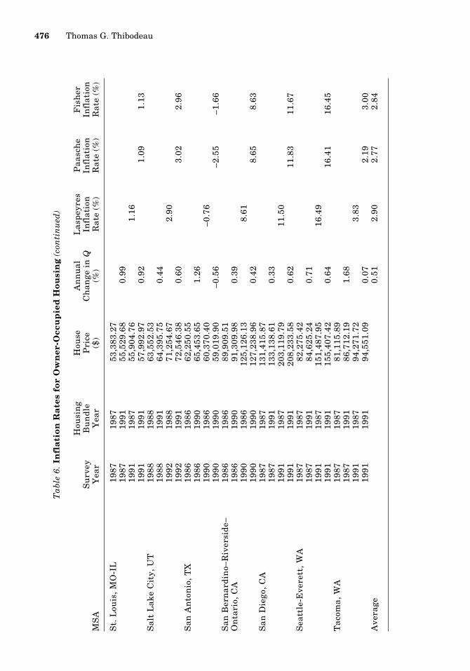
476 Thomas G. Thibodeau
Tab
le 6
. In
fla
tio
n R
ate
s fo
r O
wn
er-O
ccu
pie
d H
ou
sin
g (
con
tin
ued
)
Hou
sin
gH
ouse
An
nu
alL
aspe
yres
Paa
sch
eF
ish
erS
urv
eyB
un
dle
Pri
ceC
han
ge i
n Q
Infl
atio
nIn
flat
ion
Infl
atio
nM
SA
Yea
rY
ear
($)
(%)
Rat
e (%
)R
ate
(%)
Rat
e (%
)
St.
Lou
is,
MO
-IL
1987
1987
53,3
83.2
719
8719
9155
,529
.68
0.99
1991
1987
55,9
04.7
61.
1619
9119
9157
,992
.97
0.92
1.09
1.13
Sal
t L
ake
Cit
y, U
T19
8819
8863
,552
.53
1988
1991
64,3
95.7
50.
4419
9219
8871
,254
.67
2.90
1992
1991
72,5
46.3
80.
603.
022.
96S
an A
nto
nio
, T
X19
8619
8662
,250
.55
1986
1990
65,4
53.6
51.
2619
9019
8660
,370
.40
–0.7
619
9019
9059
,019
.90
–0.5
6–2
.55
–1.6
6S
an B
ern
ardi
no–
Riv
ersi
de–
1986
1986
89,9
09.5
1O
nta
r io,
CA
1986
1990
91,3
09.9
80.
3919
9019
8612
5,12
6.13
8.61
1990
1990
127,
238.
960.
428.
658.
63S
an D
iego
, C
A19
8719
8713
1,41
5.87
1987
1991
133,
138.
610.
3319
9119
8720
3,11
9.79
11.5
019
9119
9120
8,23
3.58
0.62
11.8
311
.67
Sea
ttle
-Eve
rett
, W
A19
8719
8782
,275
.42
1987
1991
84,6
25.2
40.
7119
9119
8715
1,48
7.95
16.4
919
9119
9115
5,40
7.42
0.64
16.4
116
.45
Tac
oma,
WA
1987
1987
81,1
15.8
919
8719
9186
,712
.19
1.68
1991
1987
94,2
71.7
23.
8319
9119
9194
,551
.09
0.07
2.19
3.00
Ave
rage
0.51
2.90
2.77
2.84
House Price Indices from the 1984–1992 MSA American Housing Surveys 477
in Houston between 1987 and 1991 (–2.38 percent). The metropolitan-area averageannualized rate of inflation in owner-occupied housing over the seven-year period was2.84 percent.
A Housing Quantity Index
The differences between the Laspeyres and Paasche indices in tables 5 and 6 suggest thatthe nation’s housing stock is changing over time. A housing quantity index was con-structed to measure the changes. Like a price index, a quantity index is the ratio of two(finite-sample-corrected) expected housing expenditures. For a quantity index, thebeginning and ending periods’ national average housing characteristics are priced usingthe same hedonic coefficients. For each metropolitan area, the quantity index is Q = pt,0/p0,0. Using 1986 Anaheim owner-occupied housing hedonic coefficients with 1990 na-tional average characteristics, the expected expenditure is $148,091.99—an increase of$5,226.69 (0.90 percent per year) over the $142,865.30 expected expenditure obtainedusing 1986 national average characteristics. Because the hedonic coefficients are heldconstant for both expected expenditures, the increase in the index value measures theincrease in the quantity/quality of the stock of housing between 1986 and 1990 (as valuedby 1986 Anaheim hedonic coefficients). The average annual rate of growth in the quantityof the nation’s owner-occupied housing stock, as valued by these metropolitan areas,between 1986 and 1992 is 0.51 percent.
Conclusion
This article reports house price indices for renter- and owner-occupied housing formetropolitan areas surveyed in the 1984–92 MSA AHS. The constant-quality house priceindices are representative of the entire stock of housing within each housing market.Price indices are computed using national average housing characteristics for residentialproperties in places with populations exceeding 100,000. Inflation rates are measuredusing Laspeyres, Paasche, and Fisher indices.
California metropolitan areas typically had the most expensive housing, while MSAs inthe South had the least expensive. Shelter rents in California MSAs were 2.5 times thosein other metropolitan areas. California owner-occupied house prices were 3 times thenational average. The average annualized rate of inflation in rents during the 1986–92period, measured using a Fisher index, was 202 basis points higher than the averageannualized rate of inflation in owner-occupied housing (4.86 versus 2.84 percent).Finally, an index of housing quantity indicates that the nation’s housing stock improvedat an average rate of 0.51 percent per year.
References
Agarwal, Vinod B., and Richard A. Phillips. 1983. The Effect of Mortgage Rate Buydowns onHousing Prices: Recent Evidence from FHA-VA Transactions. AREUEA Journal 11:45–68.
Agarwal, Vinod B., and Richard A. Phillips. 1984. Mortgage Rate Buydowns: Further Evidence.Housing Finance Review 3:191–98.
478 Thomas G. Thibodeau
Aitchison, John, and James A. C. Brown. 1957. The Lognormal Distribution. Cambridge, England:Cambridge University Press.
Blackley, Dixie M., and James R. Follain. 1987. Tests of Locational Equilibrium in the StandardUrban Model. Land Economics 63(1):46–61.
Boehm, Thomas P. 1984. Inflation and Intra-Urban Residential Mobility. Housing Finance Review3:19–38.
Bradu, Dan, and Yair Mundlak. 1970. Estimation in Lognormal Linear Models. Journal of theAmerican Statistical Association 65(329):198–211.
Cooperstein, Richard. 1989. Quantifying the Decision to Become a First-Time Home Buyer. UrbanStudies 26(2):223–33.
Crone, Theodore M. 1988. Changing Rates of Return on Rental Property and CondominiumConversion. Urban Studies 25(1):34–42.
Cronin, Francis J. 1983. Federal Tax Regulations and the Housing Demands of Owner Occupants.Land Economics 59:305–13.
DeBoer, Larry. 1985. Resident Age and Housing Search: Evidence from Hedonic Residuals. UrbanStudies 22(5):445–51.
Dhrymes, Phoebus J. 1962. On Devising Unbiased Estimators for the Parameters of the Cobb-Douglas Production Function. Econometrica 30(2):297–304.
Diewert, W. Erwin. 1976. Exact and Superlative Index Numbers. Journal of Econometrics 4:114–45.
Finney, D. J. 1941. On the Distribution of a Variate Whose Logarithm Is Normally Distributed.Journal of the Royal Statistical Society, Supplement 7(2):155–61.
Follain, James R., and Stephen Malpezzi. 1980. Dissecting Housing Value and Rent: Estimates ofHedonic Indexes for Thirty-Nine Large SMSAs. Washington, DC: The Urban Institute Press.
Follain, James R., and Stephen Malpezzi. 1981. Are Occupants Accurate Appraisers? Review ofPublic Data Use 9:47–55.
Fortura, Peter, and Joseph Kushner. 1986. Canadian Inter-City House Price Differentials.AREUEA Journal 14(4):525–36.
Gillingham, Robert. 1975. Place to Place Rent Comparisons. Annals of Economic and SocialMeasurement 4(1):153–74.
Goldberger, Arthur S. 1968. The Interpretation and Estimation of Cobb-Douglas Functions.Econometrica 36(3–4):464–72.
Goodman, Allen C. 1978. Hedonic Prices, Price Indices, and Housing Markets. Journal of UrbanEconomics 5(4):471–84.
Goodman, John L., Jr., and John B. Ittner. 1992. The Accuracy of Homeowners’ Estimates of HouseValue. Journal of Housing Economics 2(4):339–57.
Grether, David M., and Peter Mieszkowski. 1974. Determinants of Real Estate Values. Journal ofUrban Economics 1(2):127–45.
House Price Indices from the 1984–1992 MSA American Housing Surveys 479
Grether, David M., and Peter Mieszkowski. 1980. The Effects of Nonresidential Land Uses on thePrices of Adjacent Housing: Some Estimates of Proximity Effects. Journal of Urban Economics8(1):1–15.
Grootaert, Christiaan, and Jean-Luc Dubois. 1988. Tenancy Choice and the Demand for RentalHousing in the Cities of the Ivory Coast. Journal of Urban Economics 24(1):44–63.
Guntermann, Karl L., and Stefan Norrbin. 1987. Explaining the Variability of Apartment Rents.AREUEA Journal 15(4):321–40.
Hamilton, Bruce W., and Robert Schwab. 1985. Expected Appreciation in Urban Housing Markets.Journal of Urban Economics 18:103–18.
Haworth, J. M., and P. J. Vincent. 1979. The Stochastic Disturbance Specification and ItsImplications for Log Linear Regression. Environment and Planning A 11:781–90.
Heien, Dale. 1968. A Note on Log-Linear Regression. Journal of the American Statistical Associa-tion 63(323):1034–38.
Herrin, William E., and Clifford R. Kern. 1992. Testing the Standard Urban Model of ResidentialChoice: An Implicit Markets Approach. Journal of Urban Economics 31(2):145–63.
Hulten, Charles R., and Frank C. Wykoff. 1981. The Measurement of Economic Depreciation. InDepreciation, Inflation, and the Taxation of Income from Capital, ed. Charles R. Hulten, 81–125.Washington, DC: The Urban Institute Press.
Ihlanfeldt, Keith R. 1983. Property Taxation and the Demand for Housing: An EconometricAnalysis. Journal of Urban Economics 16:208–24.
Ihlanfeldt, Keith R., and Thomas Boehm. 1983. Property Taxation and the Demand forHomeownership. Public Finance Quarterly 11:47–66.
Ihlanfeldt, Keith R., and John D. Jackson. 1982. Systematic Assessment Error and IntrajurisdictionProperty Tax Capitalization. Southern Economic Journal 49:417–27.
Ihlanfeldt, Keith R., and Jorge Martinez-Vazquez. 1986. Alternative Value Estimates of Owner-Occupied Housing: Evidence on Sample Selection Bias and Systematic Errors. Journal of UrbanEconomics 20(3):356–69.
Jackson, Bryan O., and Lawrence B. Mohr. 1986. Rent Subsidies: An Impact Evaluation and anApplication of the Random-Comparison-Group Design. Evaluation Review 10(4):483–517.
Johnson, Norman L., and Samuel Kotz. 1970. Continuous Univariate Distributions. Vol. 1. NewYork: Wiley.
Kain, John, and John Quigley. 1972. Note on Owner’s Estimate of Housing Value. Journal of theAmerican Statistical Association 67(340):803–6.
Kiel, Katherine A., and Richard Carson. 1990. An Examination of Systematic Differences in theAppreciation of Individual Housing Units. Journal of Real Estate Research 5(3):301–18.
King, A. Thomas. 1973. Property Taxes, Amenities, and Residential Land Values. Cambridge, MA:Ballinger.
King, A. Thomas, and Peter Mieszkowski. 1973. Racial Discrimination, Segregation, and the Priceof Housing. Journal of Political Economy 81:590–606.
Kish, Leslie, and John Lansing. 1954. Response Errors in Estimating the Value of Homes. Journalof the American Statistical Association 49(267):520–38.

480 Thomas G. Thibodeau
Lea, Michael J., and Michael J. Wasylenko. 1983. Tenure Choice and Condominium Conversion.Journal of Urban Economics 14:127–44.
Li, Mingchi, and H. James Brown. 1980. Micro-Neighborhood Externalities and Hedonic HousingPrices. Land Economics 56(2):125–41.
Linneman, Peter D. 1980. Some Empirical Results on the Nature of the Hedonic Price Function forthe Urban Housing Market. Journal of Urban Economics 8(1):47–68.
Linneman, Peter D., and Isaac F. Megbolugbe. 1992. Housing Affordability: Myth or Reality?Urban Studies 29(3–4):369–92.
Malpezzi, Stephen, Larry Ozanne, and Thomas Thibodeau. 1980. Characteristic Prices of Housingin Fifty-nine Metropolitan Areas. Washington, DC: The Urban Institute Press.
Malpezzi, Stephen, Larry Ozanne, and Thomas Thibodeau. 1987. Microeconomic Estimates ofHousing Depreciation. Land Economics 63(4):372–85.
Manning, Christopher A. 1986. Intercity Differences in Home Price Appreciation. Journal of RealEstate Research 1(1):45–66.
Manning, Christopher A. 1989. Explaining Intercity Home Price Differences. Journal of RealEstate Finance and Economics 2(2):131–47.
Marks, Denton. 1984. The Effect of Rent Control on the Price of Rental Housing: An HedonicApproach. Land Economics 60(1):81–94.
Meulenberg, M. T. G. 1965. On the Estimation of an Exponential Function. Econometrica33(4):863–68.
Mieszkowski, Peter, and Arthur Saper. 1978. An Estimate of the Effects of Airport Noise onProperty Values. Journal of Urban Economics 5(4):425–40.
Nicholson, M., and K. Willis. 1991. Subsidies to Owner Occupiers: Some Estimates from Data onIndividual Households. Environment and Planning A 23(3):333–48.
Olsen, Edgar O. 1972. An Econometric Analysis of Rent Control. Journal of Political Economy80(6):1081–110.
Olsen, Edgar O., and David M. Barton. 1983. The Benefits and Costs of Public Housing in New YorkCity. Journal of Public Economics 20:299–332.
Ozanne, Larry. 1981. Expanding and Improving the CPI Rent Component. In House Prices andInflation, ed. John A. Tuccillo and Kevin E. Villani, 109–21. Washington, DC: The Urban InstitutePress.
Ozanne, Larry, and Thomas Thibodeau. 1983. Explaining Metropolitan Housing Price Differences.Journal of Urban Economics 13(1):51–66.
Palmquist, Raymond. 1979. Hedonic Price and Depreciation Indexes for Residential Housing: AComment. Journal of Urban Economics 6(2):267–71.
Pollakowski, Henry, Michael Stegman, and William Rohe. 1991. Rates of Return on Housing ofLow- and Moderate-Income Owners. AREUEA Journal 19(3):417–24.
Randolph, William C. 1988. Housing Depreciation and Aging Bias in the Consumer Price Index.Journal of Business and Economic Statistics 6(3):359–72.

House Price Indices from the 1984–1992 MSA American Housing Surveys 481
Reeder, William. 1985. The Benefits and Costs of the Section 8 Existing Housing Program. Journalof Public Economics 26(3):349–60.
Robins, Philip K., and Richard W. West. 1977. Measurement Errors in the Estimation of HomeValue. Journal of the American Statistical Association 72(358):290–94.
Sa-Aadu, Jarjisu. 1984a. Alternative Estimates of Direct Tenant Benefit and ConsumptionInefficiencies from the Section 8 New Construction Program. Land Economics 60:189–201.
Sa-Aadu, Jarjisu. 1984b. Another Look at the Economics of Demand-Side versus Supply-SideStrategies in Low-Income Housing. AREUEA Journal 12:427–60.
Schwab, Robert M. 1985. The Benefits of In-Kind Government Programs. Journal of PublicEconomics 27(2):195–210.
Shilling, James D., C. F. Sirmans, and Jonathan F. Dombrow. 1991. Measuring Depreciation inSingle Family Rental and Owner-Occupied Housing. Journal of Housing Economics 1(4):368–83.
Stynes, Daniel J., George L. Peterson, and Donald H. Rosenthal. 1986. Log Transformation Biasin Estimating Travel Cost Models. Land Economics 62(1):94–103.
Teekens, R., and J. Koerts. 1972. Some Statistical Implications of the Log Transformation ofMultiplicative Models. Econometrica 40(5):793–819.
Thibodeau, Thomas G. 1989. Housing Price Indexes from the 1974–1983 SMSA Annual HousingSurveys. AREUEA Journal 17(1):110–17.
Thibodeau, Thomas G. 1990. Estimating the Effect of High Rise Office Buildings on ResidentialProperty Values. Land Economics 66(4):402–8.
Thibodeau, Thomas G. 1992. Residential Real Estate Prices from the 1974–1983 StandardMetropolitan Statistical Area American Housing Survey. Studies in Urban and Resource Econom-ics. Mount Pleasant, MI: Blackstone.
U.S. Department of Housing and Urban Development. 1978. How Well Are We Housed? Washing-ton, DC: U.S. Government Printing Office.
Wieand, Kenneth F. 1983. The Performance of Annual Housing Survey Quality Measures inExplaining Dwelling Rentals in 20 Metropolitan Areas. AREUEA Journal 11:45–68.
Willis, Kenneth G., Stephen Malpezzi, and A. Graham Tipple. 1990. An Econometric and CulturalAnalysis of Rent Control in Kumasi, Ghana. Urban Studies 27(2):241–57.
Wolters, C., and H. Woltman. 1974. 1970 Census: Preliminary Evaluation Results MemorandumNo. 48. Unpublished mimeo. Washington, DC: U.S. Bureau of the Census.
Woodward, Susan E., and John C. Weicher. 1989. Goring the Wrong Ox: A Defense of the MortgageInterest Deduction. National Tax Journal 42(3):301–13.

482 Thomas G. Thibodeau