Homeowner Age and House Price AppreciationHomeowner Age and House Price Appreciation are available...

��Cityscape: A Journal of Policy Development and Research • Volume 9, Number 3 • 2007U.S. Department of Housing and Urban Development • Office of Policy Development and Research

Cityscape

Homeowner Age and House Price AppreciationDavid T. RoddaFreddie MacSatyendra PatrabanshAbt Associates Inc.

Abstract

Do the houses of elderly homeowners appreciate at the same rate as the average house in their local market? As the population ages and retirees plan their financial future, homeowners need to project accurately the value of their single largest asset—their house. The federal government is also concerned about the financial welfare of its elderly citizens and the solvency of the insurance for reverse mortgages. Using Health and Retirement Study data, we find that the houses of elderly (75 years old or older) homeowners appreciate 1 percentage point less per year in real terms than the houses of middle-aged (50 to 74 years old) homeowners. These estimates are smaller than the findings of Davidoff (2004), who used the American Housing Survey to show a 3-percentage-point slower house appreciation rate for homeowners aged 75 or older relative to that of all other homeowners. Using census microdata in nonlongitudinal form (1990 and 2000), we find 2.4-percentage-point slower real house appreciation for elderly homeowners. Houses of elderly homeowners thus appreciate in real terms at a 1- to 3-percentage-point discount relative to their local markets.

IntroductionDo the houses of elderly homeowners appreciate at the same rate as the average house in their local market? The answer matters most directly to elderly homeowners making long-range financial plans. For most elderly homeowners, and especially for low-wealth homeowners, their house is

Funding for this research was provided by the U.S. Department of Housing and Urban Development (HUD), Office of Policy Development and Research, Contract C-OPC-21452 RG. Additional funding was provided by Abt Associates Inc. through a Daniel T. McGillis Development and Dissemination Grant. The opinions expressed in this paper are the authors’ own and do not represent HUD, Abt Associates, or Freddie Mac.

�� Refereed Papers

Rodda and Patrabansh

their largest asset. It would be logical to assume that the house would appreciate at the long-run average house price appreciation rate (5.9 percent per year in nominal terms minus 4.1 percent for inflation equals 1.8 percent in real terms).1 Despite this assumption, elderly homeowners might have lower house appreciation rates because they spend less money on remodeling and maintenance. Most people know of an old person who has lived in the same house for many years and done little to update the property. Does this anecdotal evidence represent an outlier or should elderly homeowners expect lower house price appreciation?

Elderly homeowners are not the only ones concerned about their house values and financial planning. Certainly their children have a vested interest in providing for their parents. Local governments rely on property taxes linked to house values. Towns with a high proportion of elderly homeowners have to provide sufficient social services, particularly for seniors who prefer to stay in their own homes. Both the families and their local governments want to preserve the older properties as a source of affordable housing for the next generation of homebuyers. Finally, the federal government cares about elderly homeowners and their house values. In particular, the Federal Housing Administration insures Home Equity Conversion Mortgages (HECMs), which enable elderly homeowners to convert their house equity into cash. The homeowners do not need to pay off the reverse mortgage until they move or permanently leave their home; at that point, the house is sold to pay off the loan. The long-run viability of the HECM insurance fund depends on projected house values exceeding loan balances. Given the potentially long time horizon of 20 years or more before the loan is paid, what should government officials assume about future house price appreciation?

Using data from Growing Older in America: The Health and Retirement Study (HRS), we find that the houses of elderly (75 years or older) homeowners appreciate in constant dollars at a rate 1.0 to 1.2 percentage points less per year than the houses of middle-aged (50 to 74 years old) homeown-ers. This discount in house price appreciation for age is smaller than the 3-percentage-point dis-count estimated in Davidoff (2004) using American Housing Survey (AHS) data. Our HRS estimate compares house value appreciation for elderly homeowners with that of middle-aged homeowners for a period of 10 years or less, while Davidoff’s (2004) AHS estimates contrast house value ap-preciation for elderly homeowners with that for all homeowners and follows the homeownership period for up to 16 years. After adjusting the HRS estimates for the 0.4-percentage-point gap between middle-aged homeowners and all homeowners, our best estimate for the elderly discount in house value appreciation is 1.4 to 1.6 percentage points relative to all homeowners.

Both the HRS and AHS data sets are longitudinal. Longitudinal data sets enable us to control for fixed personal and property-specific effects and provide the best way to track the change in house values without the confounding effects of the changing composition of households and properties. The appreciation rate can also be tracked using the Census Bureau’s Public Use Microdata Sample (PUMS). PUMS has a disadvantage in that it consists of two independent cross-sections, 1990 and 2000, which were aggregated by age group and metropolitan statistical area (MSA). PUMS data have large samples and better controls for building age and length of tenure than those that

1 The 5.9-percent annual house price appreciation rate comes from the Office of Federal Housing Enterprise Oversight (OFHEO) national House Price Index from the first quarter of 1975 to the first quarter of 2005. The inflation rate of 4.1 percent is calculated from the Consumer Price Index excluding shelter expenses for the same period.

��Cityscape

Homeowner Age and House Price Appreciation

are available in the HRS data. PUMS data indicate that the house prices of homeowners 75 years old and older appreciate 2.4 percentage points more slowly per year than do those of younger homeowners.

Thus, two independent studies, this one and Davidoff’s (2004), analyzing three separate data sets—HRS, AHS, and PUMS—show a negative and significant relationship between age and house value appreciation. The elderly discount from the HRS is about half the discount from the AHS or PUMS, but even that smaller difference could be critical in the long run to homeowners, lenders, and insurance funds (see exhibit 5 in the second section following this introduction).

The remainder of the article is divided into four sections. The first section provides a brief review of the literature on elderly housing decisions. The second section presents the HRS data used for analysis and ends with estimations of house value appreciation using HRS/Assets and Health Dynamics Among the Oldest Old (AHEAD) Study data and comparisons with recent findings by Davidoff (2004) using the AHS data. The third section provides a benchmark from the Census Bureau’s PUMS data by comparing appreciation rates between 1990 and 2000. A final section summa-rizes the findings in light of six alternative “stories,” each of which may contain some partial truth.2

Literature ReviewSeveral authors have addressed the issue of elderly wealth. Venti and Wise (2001a, 2001b) have used HRS/AHEAD data to find that equity-rich, low-income households tend to reduce equity when they sell. People with substantial amounts of nonhousing wealth shift their assets into housing, whereas people with limited nonhousing wealth rebalance their portfolio by reducing the housing equity share. Overall, housing equity increases until about age 75 and then declines by about 1.76 percent per year. Homeowners with intact households rarely move or refinance to take equity out of their house. The equity decline among older homeowners is driven primarily by 7.84 percent of households experiencing a health shock (either a death or move to a nursing home) to their family status.

The life-cycle model (Hurd, 1990) predicts that wealth will be “decumulated” as people age, but the uncertainty about the amount of time until death leads people to spend down nonhous-ing wealth first and hang onto their house as long as possible. In fact, the results confirm that nonhousing wealth is spent down faster and earlier than home equity. Owned housing is not just an investment; it also provides a stream of real consumption and precautionary savings against unexpected costs, especially health costs (Heiss, Hurd, and Borsch-Supan, 2003).

Goodman and Thibodeau (1997, 1995) found that the largest reduction in house value from depreciation occurs in the first 10 years of the building’s life before tapering off to 0 when the building reaches age 20 and slightly increasing in years 20 to 40, presumably due to remodeling. (See also Harding, Rosenthal, and Sirmans, 2007.) The findings by Goodman and Thibodeau (1997, 1995) suggest that old buildings do not suffer greater depreciation as the homeowner

2 The full report, The Relationship Between Homeowner Age and House Price Appreciation, which includes policy implications and statistical appendixes, is available on the Abt Associates Inc. website (http://www.abtassociates.com/reports/HP_Aging_Final.pdf).



ages, but the extremely aged homeowners were probably a small share of the sample. Even more consistent in their findings than the rate of depreciation is the widening variance in house values as buildings age. The range of house values for an old building is usually much wider than for a new house. Part of this age-related heteroskedasticity is due to home improvement projects, including additions and remodeling. Capozza, Israelsen, and Thomson (2005) refer to the “atypicality” of a house that has acquired unusual features as it has aged. Appraisers may have a difficult time finding comparable houses in the neighborhood and therefore discount the appraised value. Older homeowners often have not updated the style of their house for 10 to 20 years, and, as a result, the house becomes atypical relative to other houses on the market. The dated styles lower demand and increase the search time for a suitable buyer, leading to discounts for atypical houses. These find-ings directly support the fifth explanation for elderly discounts: the higher variance of older house values is a leading cause of lower appreciation rates for older homeowners.

The most relevant predecessor to this article is by Davidoff (2004). He used the panel of national AHS data from 1985 to 2001 both to measure the house price appreciation of homes owned by the elderly and to link maintenance spending to homeowner age. He found that elderly homeowners spend less on maintenance. Homeowners who are more than 75 years old spend $270 less on routine maintenance than do younger homeowners of similar homes and spend $1,100 less on all home improvements. Older homeowners also realize lower house price appreciation by about 3 percent per year than do younger homeowners for similar homes in similar markets during 1985 to 2001.

Most of the house value data that are publicly available use information reported by the homeown-ers. How reliable are the self-reported house values by elderly homeowners? Using the national AHS (1985 to 1987), Goodman and Ittner (1992) found that the average homeowner overvalues his or her house by 6 percent, with an average absolute error rate of 14 percent. DiPasquale and Somerville (1995) used the AHS data to compare the rate of appreciation in house prices based on transaction units with the entire stock. They found that units with longer tenure had lower house values and lower appreciation.

Kiel and Zabel (1999) used confidential metropolitan AHS data merged with census tract-level information for the neighborhood around each unit. They found that recent buyers report house values that are 8.4 percent higher than the eventual sales price, whereas homeowners with longer tenure overvalue their houses by only 3.3 percent.3 Kiel and Zabel (1999) estimated that the self-reports were, on average, 5.1 percent too high, but the upward bias was not related to the characteristics of the house, occupants (except for tenure), or neighborhood. Also, the upward bias on homeowners’ valuations seems to decline with the length of tenure. When Kiel and Zabel (1999) controlled for maintenance or remodeling, the difference between value and sales price fell by 1 percentage point.

3 Fisher and Williams (2006) offer one explanation for high estimates of recent buyers. Basing their analysis on Consumer Expenditure Survey data, they found a spike in additions and maintenance spending in the first 3 years of ownership.

��Cityscape


The Health and Retirement Study Data and ModelsThe HRS/AHEAD4 is a particularly useful data source for investigating the relationship between a homeowner’s age and the rate of house value appreciation. Many studies, particularly longitudinal ones, have very little coverage of the elderly population because this segment is out of the labor force and has previously represented a small share of the population. The HRS/AHEAD, however, focuses on the near-retirement and elderly populations and surveys them roughly every 2 years. The survey includes variables on family structure, living arrangements, retirement decisions, financial state, and health status. As a source on housing data, it has not been used nearly as much as the AHS. The HRS/AHEAD provides opportunities to corroborate findings from other studies and further their analyses on elderly health and wealth issues.

The HRS tracks the same households as they enter retirement and experience the health challenges of aging. HRS began with a longitudinal sample of more than 12,600 people in 7,600 households who were born in the period from 1931 through 1941; the people in this sample were 51 to 61 years old when the initial survey occurred in 1992. Followup surveys of the same households were conducted in even years until 1998, when HRS was merged with AHEAD. AHEAD surveyed 7,447 people in about 6,000 households in which one member was born before 1923; that is, one member of the household was 70 years old or older when the initial survey was conducted in 1993. A followup survey was conducted in 1995. Both HRS and AHEAD oversampled African Americans, Hispanics, and Florida residents.5 In 1998, two new birth cohorts were added: Children of the Depression Age (CODA), born between 1924 and 1930, and War Babies (WBs), born between 1942 and 1947. Moreover, additions from new relationships and remarriages are made in each followup survey. Therefore, the current HRS/AHEAD/CODA/WBs sample exceeds 22,000 people and 14,000 households; more than 18,000 people in more than 12,000 households were interviewed in 2002.

Sample SelectionTo select our sample, we used the HRS tracker and region files prepared in 2002 in conjunction with the core HRS/AHEAD survey files of each even year from 1992 through 2002 and the years 1993 and 1995. We identified nearly 12,000 households that owned a single-family, nonfarm, nonmobile,6 noncondominium primary home in at least 1 survey year from 1992 through 2002. House values were self-reported by the financial respondent in each wave. About 9,500 of those households were observed in at least 2 survey years in the same primary home, providing two dif-ferent snapshots of house values and other mutable characteristics of the same home and the same homeowners at two distinct points in time. Because our unit of analysis is a primary home and because some households are observed in more than one distinct primary home between 1992 and

4 The Health and Retirement Study (HRS) merged with the Assets and Health Dynamics Among the Oldest Old (AHEAD) Study in 1998; now the studies are collectively referred to as HRS/AHEAD or simply HRS.5 In part, because of this oversampling by race and location, weights are used throughout the analysis. If weights were insufficient to restore the representativeness of the data, it is possible that the lower house price appreciation found in the Health and Retirement Study results are linked to the sampling.6 The Health and Retirement Study uses the term “mobile homes,” which we interpret as essentially synonymous with manufactured housing. To be consistent with the survey coding, however, we refer to mobile homes in this article.



2002, the number of unique single-family, nonfarm, nonmobile, noncondominium owned primary homes observed in at least 2 different survey years is 10,129.7 After imputation for missing data and the conversion of dollar amounts to 2002 dollars using the seasonally unadjusted Consumer Price Index excluding shelter expenses for all urban consumers, we calculated the compound annual growth rate (CAGR) of house values.

Description of HRS DataDemographic characteristics are available from both the core survey files and the tracker file. As recommended by HRS, we used the data from the tracker file as much as possible. To obtain person information at the household level, we used the characteristics of the financial respondent.8 When the financial respondent could not be identified or when the household did not participate in the financial section of the surveys in the wave we were interested in, we used the characteristics of the family respondent. We obtained fixed characteristics such as the date of birth, gender, race, and ethnicity of the financial respondent or the family respondent from the tracker file. Some demographic characteristics, such as whether respondents are in a nursing home and their coupled status, change over time. In many instances, we used the characteristics from the end year, also available from the tracker file. We also obtained the household weights from the tracker file.

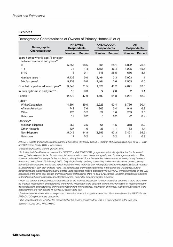
In exhibit 1, we summarize demographic characteristics of homeowners. It should be noted that some homeowners who are represented in multiple homes are counted multiple times in our sam-ple of unique homes. No household appears more than three times and 88 percent of households appear only once, as shown by the home sequence number in exhibit A-1 (see the appendix at the end of the article). Almost all family respondents are financial respondents; that is, they answered the financial sections of the survey.

We selected 75 years of age as our breakpoint for analysis because Venti and Wise (2001a, 2001b) show that housing equity increases for homeowners until about age 75 and then declines. At both the starting year and the ending year, only a few family respondents for the HRS/WBs group were 75 years old or older and almost no family respondents for the AHEAD/CODA group were younger than 65. The percentages of homeowners who were 75 years old or older in the start year are almost 0 for the HRS/WBs group and 36 for the AHEAD/CODA group; this comparison grows even more pronounced in the end year. Even though some overlap occurs in the near-elderly age group of 65 to 74 years between the HRS/WBs and AHEAD/CODA groups, tabulating the characteristics of the HRS/WBs group with those of the AHEAD/CODA group provides a good way to compare the middle-aged or near-retirement family respondents with the elderly family respondents.

Besides homeowner age, the main distinctions in exhibit 1 between the middle-aged (HRS/WBs) and the elderly (AHEAD/CODA) respondents are as follows:

7 We extracted values from the waves when the home was first and last observed and called them starting and ending house values. Even though the Health and Retirement Study survey wave years are 1992, 1993, 1994, 1995, 1996, 1998, 2000, and 2002, actual interview years range from 1991 to 2003. We call the actual interview years of first and last observation as our start (interview) years and end (interview) years, respectively. Dollar adjustments to 2002 dollars are made on the basis of interview years, not wave years. See the appendix for more details.8 The financial respondent is the person responsible for overseeing the financial matters of the elderly person, often the elderly person himself or herself and usually the same person as the family respondent. If the financial respondent information was missing, the family respondent information (some other person from the same family) was substituted.

��Cityscape


Exhibit 1

DemographicCharacteristicsa

HRS/WBsRespondents

AHEAD/CODA Respondents

AllRespondents

Number Percent Number Percent Number Percent

Demographic Characteristics of Owners of Primary Homes (1 of 2)

Respondent type**Financial 5,403 99.4 2,461 99.9 7,864 99.6Family 36 0.6 3 0.1 39 0.4

Age in start year**54 or younger 2,198 46.7 10 0.5 2,208 32.355–64 2,907 48.0 44 2.6 2,951 33.865–74 325 5.1 1,466 60.7 1,791 22.575–84 9 0.2 802 31.6 811 10.085 or older 0 0.0 142 4.6 142 1.5

Average age** 5,439 55.4 2,464 73.8 7,903 61.1Median ageb 5,439 56.0 2,464 73.0 7,903 59.0

Age in end year**54 or younger 506 11.5 3 0.1 509 7.955–64 2,968 59.3 16 1.1 2,984 41.265–74 1,847 27.1 477 20.4 2,324 25.075–84 116 2.0 1,487 61.0 1,603 20.485 or older 2 0.0 481 17.4 483 5.5

Average age** 5,439 61.0 2,464 79.1 7,903 66.7Median ageb 5,439 62.0 2,464 79.0 7,903 66.0

• More HRS/WBs group households than AHEAD/CODA group households are couples (71.5 compared with 41.2 percent).

• Fewer HRS/WBs group households than AHEAD/CODA group households are headed by females (47.9 compared with 61.8 percent).

• Fewer HRS/WBs group households than AHEAD/CODA group households are headed by Whites (89.0 compared with 93.4 percent).

The younger cohort is more likely to live in the South Atlantic Census Division (22.3 percent compared with 18.3) and have much shorter average tenure (15.8 years compared with 26.0). In terms of financial and health characteristics, the younger cohort is more likely to own a second home (15.2 percent compared with 8.8) but has lower average liquid assets ($179,559 compared with $192,241) and lower medical expenses ($2,055 compared with $2,837). HRS does not include direct measurement of maintenance expenditures, but home improvements or major additions are reported in exhibit 2. The younger cohort has a higher percentage of home improvements (26.9 percent compared with 19.2) and a higher average biannual home improvement cost ($4,084 compared with $2,826). Even though the older households have more liquid assets, they spend less on home improvements and perhaps also on maintenance, which is not itself reported. House price appre-ciation (measured by the CAGR in constant 2002 dollars) is shown in exhibit 2. The distributions of growth rates range widely, but the average CAGR is significantly higher for the younger cohort than for the elderly (2.28 percent compared with 1.52). Without a regression adjustment, the aver-age house price appreciation is about 0.75 percentage point lower for the elderly homeowners.

��0 Refereed Papers


AHEAD = Assets and Health Dynamics Among the Oldest Old Study. CODA = Children of the Depression Age. HRS = Health and Retirement Study. WBs = War Babies.

*Indicates significance at the 5-percent level.

**Indicates that the differences between the HRS/WB and AHEAD/CODA groups are statistically significant at the 1-percent level. χ2 tests were conducted for cross-tabulation comparisons and t-tests were performed for average comparisons. The observation level of the sample in this article is a primary home. Some households have as many as three primary homes in the survey period from 1992 through 2002. Only single-family, nonfarm, nonmobile, and noncondominium owned primary homes are considered in the sample, which is also confined to homes with nonimputed and nonmissing house values reported by respondents in both start and end years. The sample sizes and medians presented in this exhibit are unweighted, but the percentages and averages reported are weighted using household weights provided by HRS/AHEAD to make inference on the U.S. population of the same age, gender, and race/ethnicity profile as that of the HRS/AHEAD sample. All dollar amounts are adjusted to 2002 using the nonseasonally adjusted Consumer Price Index excluding shelter expenses.a From the tracker and region files, characteristics of the financial respondent for each wave was obtained. Where there were no financial respondents, characteristics of the family respondent were obtained. Where the information on respondent type was unavailable, characteristics of the oldest respondent were obtained. Information on homes, such as house values, were obtained from the year-specific HRS/AHEAD survey data files.b Medians are calculated without weights and no statistical tests for significance of the difference between the HRS/WBs and AHEAD/CODA groups were conducted.c This variable captures whether the respondent or his or her spouse/partner was in a nursing home in the end year.

Source: 1992 to 2002 HRS/AHEAD

Years homeowner is age 75 or older between start and end years**

0 5,357 98.5 665 28.1 6,022 76.51–5 74 1.4 1,151 46.4 1,225 15.46–10 8 0.1 648 25.5 656 8.1

Average years** 5,439 0.0 2,464 3.3 7,903 1Median yearsb 5,439 0.0 2,464 3.0 7,903 0.0

Coupled or partnered in end year** 3,843 71.5 1,028 41.2 4,871 62.0

In nursing home in end year** c 18 0.3 74 2.8 92 1.1

Female** 2,772 47.9 1,509 61.8 4,281 52.2

Race**White/Caucasian 4,504 89.0 2,226 93.4 6,730 90.4African American 742 7.6 206 5.4 948 6.9Other 176 3.2 27 1.0 203 2.5Unknown 17 0.2 5 0.2 22 0.2

Ethnicity**Mexican Hispanic 253 3.5 65 1.5 318 2.9Other Hispanic 127 1.6 36 1.1 163 1.4Non-Hispanic 5,042 94.8 2,359 97.3 7,401 95.5Unknown 17 0.2 4 0.2 21 0.2

Exhibit 1

Demographic Characteristics of Owners of Primary Homes (2 of 2)

DemographicCharacteristicsa

HRS/WBsRespondents


AllRespondents

Number Percent Number Percent Number Percent

��Cityscape


AHEAD = Assets and Health Dynamics Among the Oldest Old Study. CAGR = compound annual growth rate. CODA = Children of the Depression Age. HRS = Health and Retirement Study. WBs = War Babies.

* Values in this column are in percent unless designated by a dollar sign.

** Indicates that the differences between the HRS/WB and AHEAD/CODA groups are statistically significant at the 1-percent level. χ2 tests were conducted for cross-tabulation comparisons and t-tests were performed for average comparisons. The observation level of the sample in this article is a primary home. Some households have as many as three primary homes in the survey period from 1992 through 2002. Only single-family, nonfarm, nonmobile, and noncondominium owned primary homes are considered in the sample, which is also confined to homes with nonimputed and nonmissing house values reported by respondents in both start and end years. The sample sizes and medians presented in this exhibit are unweighted, but the percentages and averages reported are weighted using household weights provided by HRS/AHEAD to make inference on the U.S. population of the same age, gender, and race/ethnicity profile as that of the HRS/AHEAD sample. All dollar amounts are adjusted to 2002 using the nonseasonally adjusted Consumer Price Index excluding shelter expenses.a From the tracker and region files, characteristics of the financial respondent for each wave were obtained. Where there were no financial respondents, characteristics of the family respondent were obtained. Where the information on respondent type was unavailable, characteristics of the oldest respondent were obtained. Information on homes, such as house values, was obtained from the year-specific HRS/AHEAD survey data files.b CAGR = (FV/PV)1/n – 1, where PV is the beginning value, FV is the ending value, and n is the number of intervening years. This measure is very similar to ln(FV/PV)/n, which assumes continous compounding. We prefer CAGR because most house price growth rates, like interest rate growth rates, are reported in annual growth rates.c Medians are calculated without weights and no statistical tests for significance of the difference between the younger and older groups were conducted.


Home Improvement or Major Additiona

Reported in end year**

Yes 1,388 26.9 463 19.2 1,851 24.5

No 4,039 72.9 1,995 80.6 6,034 75.3

Unknown 12 0.2 6 0.2 18 0.2

Average biannual home improvement costs

5,392 $4,084 2,442 $2,826 7,834 $3,691

Median biannual home improvement costs

5,392 $ 0 2,442 $ 0 7,834 $ 0

House Price Appreciation

CAGRb of primary home**

– 10.00% or less 173 2.8 116 4.6 289 3.3

– 10.01% to – 5.00% 271 4.8 135 5.5 406 5.0

– 5.01% to – 3.00% 222 3.9 130 4.9 352 4.2

– 3.01% to – 1.00% 848 14.8 484 19.2 1,332 16.2

– 1.01% to 0.00% 511 8.8 192 7.9 703 8.6

0.01% to 1.00% 507 8.8 219 9.1 726 8.9

1.01% to 3.00% 1,057 18.6 370 15.0 1,427 17.5

3.01% to 5.00% 680 12.9 275 11.5 955 12.5

5.01% to 10.00% 742 15.5 311 12.9 1,053 14.7

10.01% or more 428 9.1 232 9.5 660 9.2

Average CAGR of primary home** 5,439 2.28 2,464 1.52 7,903 2.04

Median CAGR of primary homec 5,439 1.30 2,464 0.73 7,903 1.19

Exhibit 2

Home Improvement and House Price Appreciation

HRS/WBsRespondents


AllRespondents

Number Percent* Number Percent* Number Percent*



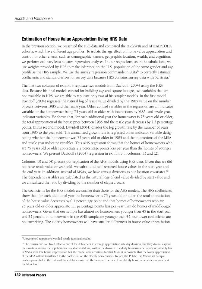
Estimation of House Value Appreciation Using HRS DataIn the previous section, we presented the HRS data and compared the HRS/WBs and AHEAD/CODA cohorts, which have different age profiles. To isolate the age effect on home value appreciation and control for other effects, such as demographic, tenure, geographic location, wealth, and cognition, we perform ordinary least squares regression analyses. In our regressions, as in the tabulations, we use weights provided by HRS to make inference on the U.S. population of the same gender and age profile as the HRS sample. We use the survey regression commands in Stata® to correctly estimate coefficients and standard errors for survey data because HRS contains survey data with 52 strata.9

The first two columns of exhibit 3 replicate two models from Davidoff (2004) using the HRS data. Because his final models control for building age and square footage, two variables that are not available in HRS, we are able to replicate only two of his simpler models. In the first model, Davidoff (2004) regresses the natural log of resale value divided by the 1985 value on the number of years between 1985 and the resale year. Other control variables in the regression are an indicator variable for the homeowner being 75 years old or older with interactions by MSA, and resale year indicator variables. He shows that, for each additional year the homeowner is 75 years old or older, the total appreciation of the house price between 1985 and the resale year decreases by 2.3 percentage points. In his second model, Davidoff (2004) divides the log growth rate by the number of years from 1985 to the year sold. The annualized growth rate is regressed on an indicator variable desig-nating whether the homeowner was 75 years old or older in 1985 and the interactions of the MSA and resale year indicator variables. This AHS regression shows that the homes of homeowners who are 75 years old or older appreciate 2.2 percentage points less per year than the homes of younger homeowners. We present Davidoff’s (2004) regression in exhibit 3 in columns (1) and (2).

Columns (3) and (4) present our replication of the AHS models using HRS data. Given that we did not have resale value or year sold, we substituted self-reported house values in the start year and the end year. In addition, instead of MSAs, we have census divisions as our location covariates.10 The dependent variables are calculated as the natural logs of end value divided by start value and we annualized the ratio by dividing by the number of elapsed years.

The coefficients for the HRS models are smaller than those for the AHS models. The HRS coefficients show that, for each additional year the homeowner is 75 years old or older, the total appreciation of the house value decreases by 0.7 percentage point and that homes of homeowners who are 75 years old or older appreciate 1.1 percentage points less per year than do homes of middle-aged homeowners. Given that our sample has almost no homeowners younger than 45 in the start year and 35 percent of homeowners in the AHS sample are younger than 45, our lower coefficients are not surprising. The elderly homeowners will have smaller differences in house value appreciation

9 Unweighted regressions yielded nearly identical results.10 The census division fixed effects control for differences in average appreciation rates by division, but they do not capture the variation among metropolitan statistical areas (MSAs) within the division. If elderly homeowners disproportionately live in MSAs with low house appreciation but the model omits controls for that MSA, it is possible that the lower appreciation of the MSA will be transferred to the coefficient on the elderly homeowners. In fact, the Public Use Microdata Sample models presented in the text and the exhibits show that the negative coefficient on elderly homeowners is even greater at the MSA level.

��Cityscape


AH

EAD

= A

sset

s an

d H

ealth

Dyn

amic

s A

mon

g th

e O

ldes

t Old

Stu

dy. A

HS

= A

mer

ican

Hou

sing

Sur

vey.

CA

GR

= c

ompo

und

annu

al g

row

th r

ate.

HR

S =

Hea

lth a

nd R

etire

men

t Stu

dy.

M

SA

= m

etro

polit

an s

tatis

tical

are

a.

**In

dica

tes

sign

ifica

nce

at th

e 1-

perc

ent l

evel

.a A

HS

resu

lts a

re fr

om D

avid

off (

2004

).b

The

obse

rvat

ion

leve

l of t

he s

ampl

e in

this

repo

rt is

a p

rimar

y ho

me.

Som

e ho

useh

olds

hav

e as

man

y as

thre

e pr

imar

y ho

mes

in th

e su

rvey

per

iod

from

199

2 th

roug

h 20

02. O

nly

sing

le-

fam

ily, n

onfa

rm, n

onm

obile

, and

non

cond

omin

ium

ow

ned

prim

ary

hom

es a

re c

onsi

dere

d in

the

sam

ple,

whi

ch is

als

o co

nfine

d to

hom

es w

ith n

onim

pute

d an

d no

nmis

sing

hou

se v

alue

s re

port

ed b

y re

spon

dent

s in

bot

h st

art a

nd e

nd y

ears

. CA

GR

, the

dep

ende

nt v

aria

ble,

is a

mea

sure

sim

ilar

to a

nnua

lized

diff

eren

ce in

nat

ural

logs

of e

nd a

nd s

tart

val

ues

in (4

). R

esul

ts a

re

wei

ghte

d to

mak

e in

fere

nce

on th

e U

.S. p

opul

atio

n of

the

sam

e ag

e, g

ende

r, an

d ra

ce/e

thni

city

pro

file

as th

at o

f the

HR

S/A

HEA

D s

ampl

e us

ing

hous

ehol

d w

eigh

ts p

rovi

ded

by H

RS

. All

dolla

r am

ount

s ar

e ad

just

ed to

200

2 us

ing

the

nons

easo

nally

adj

uste

d C

onsu

mer

Pric

e In

dex

excl

udin

g sh

elte

r ex

pens

es.

c Dav

idof

f (20

04) c

alls

this

var

iabl

e YE

AR

Sa7

5. H

is s

tart

yea

r is

198

5 an

d en

d ye

ar is

the

actu

al y

ear

whe

n th

e ho

me

was

sol

d.d

Dav

idof

f (20

04) c

alls

this

var

iabl

e a7

5. H

is s

tart

yea

r is

198

5.

Sou

rce:

199

2 to

200

2 H

RS

/AH

EAD

Year

s ag

e 75

or

old

er b

etw

een

st

art

and

end

yea

rsc

–

0.02

3

– 0.

0074

–

0.00

23

(0

.009

) *

(0.0

018)

**

(0.0

003)

**

Age

75

or o

lder

in s

tart

yea

rd

– 0.

022

–

0.01

07

– 0.

0103

(0

.016

)

(0.0

029)

**

(0.0

028)

**

Con

stan

t

0.16

7

0.02

6

0.23

9

0.04

3

0.04

7

0.04

6

(0

.013

) **

(0

.004

) **

(0

.055

) **

(0

.013

) **

(0

.015

) **

(0

.015

) **

Fixe

d e

ffect

sM

SA

xye

ar s

old

MS

A x

year

sol

dD

ivis

ion

xen

d y

ear

Div

isio

n x

end

yea

rD

ivis

ion

x en

d y

ear

Div

isio

n x

end

yea

r

N

2,78

1

2,75

7

7,30

9

7,30

9

7,30

9

7,30

9

R2

0.

36

0.30

0.

08

0.07

0.

06

0.06

Exh

ibit

3

AH

Sa

HR

S/A

HE

AD

b

(1)

(2)

(3)

(4)

(5)

(6)

lnR

esal

e Va

lue

InR

esal

e Va

lue

lnE

nd V

alue

InE

nd V

alue

CA

GR

CA

GR

1985

Val

ue19

85 V

alue

Sta

rt V

alue

Sta

rt V

alue

Year

So

ld –

198

5E

nd –

Sta

rt Y

ear

Com

par

ison

of H

RS

/AH

EA

D R

egre

ssio

ns W

ith A

HS

Reg

ress

ions



when compared with the appreciation rates of the near-elderly and the middle-aged homeowners than when compared with the appreciation rates of the general population of homeowners.11

Given that house value appreciation can have both location and time variations, some differences in the magnitude of AHS and HRS coefficients can be expected because HRS has a different and

AHEAD = Assets and Health Dynamics Among the Oldest Old Study. CAGR = compound annual growth rate. HRS = Health and Retirement Study. TICS = Telephone Interview for Cognitive Status.

* Indicates significance at the 5-percent level.

** Indicates significance at the 1-percent level. The observation level of the sample in this report is a primary home. Some households have as many as three primary homes in the survey period from 1992 through 2002. Only single-family, nonfarm, nonmobile, and noncondominium owned primary homes are considered in the sample, which is also confined to homes with nonimputed and nonmissing house values reported by respondents in both start and end years. CAGR, the dependent variable, is a measure similar to annualized difference in natural logs of end and start values. Results are weighted to make inference on the U.S. population of the same age, gender, and race/ethnicity profile as that of the HRS/AHEAD sample using household weights provided by HRS. All dollar amounts are adjusted to 2002 using the nonseasonally adjusted Consumer Price Index excluding shelter.


Respondent older than 74 years in start year

– 0.0121 0.0028** – 0.0097 0.0029** – 0.0098 0.0029**

Interval between end and start years

– 0.0027 0.0004** – 0.0027 0.0004**

Suburban location of home

– 0.0060 0.0023** – 0.0060 0.0023**

Rural location of home – 0.0062 0.0024** – 0.0063 0.0024**

Liquid assets indicator 0.0082 0.0038* 0.0082 0.0038*

TICS score less than 5 – 0.0060 0.0078

TICS score missing 0.0039 0.0047

Mexican-Hispanic respondent

– 0.0117 0.0060 – 0.0117 0.0060

Other Hispanic respondent

– 0.0057 0.0069 – 0.0056 0.0069

Constant 0.0218 0.0010** 0.0607 0.0159** 0.0603 0.0156**

Fixed effects None Division x end year

Division xend year

Other covariates None Yes Yes

N 7,903 7,903 7,903

R2 0.00 0.08 0.08

Exhibit 4

Covariate

(11) (14) (16)

CoefficientStandard

ErrorCoefficient

Standard Error

CoefficientStandard

Error

Regressions of Compound Annual Growth Rates of House Values

11 In addition, the American Housing Survey (AHS) maximum observation period for a home is 16 years, between 1985 and 2001, while the Health and Retirement Study (HRS) maximum observation period is 10 years, between 1992 and 2002. A large number of homes in the HRS are observed for shorter periods than 10 years and owners may not adjust their perceptions of house values in shorter time horizons (HRS) as much as in longer time horizons (AHS).

��Cityscape


shorter timeframe, and its geographic breakdown is not as detailed. The inability of the census division indicator variables to pick up location variation as much as the MSA indicator variables shows up as a lower R-squared in the HRS models compared with the AHS models.

Instead of the log difference of house values, we prefer to use the CAGR of house values. The log difference assumes continuous compounding; CAGR, on the other hand, reports annual growth rate similar to that of interest rates and is suitable for house value growth rates. Despite these differences, the two measures are more alike than different in terms of computation.12 In regression models (5) and (6), we used CAGR of house values as the dependent variable and the similarity of annualized log difference and CAGR becomes evident by comparing the coefficients of the age indicator variable in regression models (4) and (6). They are essentially the same.

Regression model (6) serves as the HRS foundation model for further specification testing. In exhibit 4, we estimate the same regression without the interactions between the end years and census division indicator variables in regression model (11). The two coefficients are very close but the R-squared of regression model (11) is practically 0. The interaction indicator variables do not influence the age effect but explain some location variations to make the regression a better fit. As more covari-ates were added to the model, the coefficient of age decreased very slightly in magnitude but its significance remained strong. The Telephone Interview for Cognitive Status (TICS)13 score did not have a significant coefficient and the coefficient on age barely changed from -0.0097 to -0.0098. The 1.0-percentage-point decrease in annual house value appreciation rate for elderly homeowners is a lower bound of the estimate. The upper bound is a 1.2-percentage-point decrease in CAGR, as shown in regression model (11).

Other significant covariates in the regressions included the interval between the start year and the end year, the suburban and rural location of a home compared with an urban location, the pres-ence of liquid assets, the TICS score, and the homeowner’s being Mexican Hispanic. The longer the interval between the start year and the end year, the lower the annual house appreciation is. Suburban and rural homes have lower annual appreciation than do urban homes, presumably because urban land values are appreciating more rapidly. Homes owned by individuals possessing liquid assets have higher annual appreciation. The significance of the Mexican-Hispanic indicator variable is consistent across models while no other demographic variable is significant. Homes with Mexican-Hispanic homeowners apparently have lower annual appreciation. This control variable may be picking up a neighborhood effect that the census division variables are not able to pick up.

A graphical representation of how lower appreciation rates affect the values of homes over 20 years is shown in exhibit 5. The homeowner types include the following:

12 If a house value is $100,000 for 1992 and $250,000 for 2002, in real terms, the compound annual growth rate is 9.6 percent, while the annualized log difference is 9.2 percent, and the log difference is 91.6 percent. Compare those rates to a crude percentage change of 150 percent and a percentage change per year of 11. Each approach measures the same change from $100,000 to $250,000, but the 9.6 percent for the compound annual growth rate emphasizes the effect of simple annual interest compounding over time. 13 The TICS score is a standard multidimensional measure of cognitive function, including mental acuity and memory. The values range from 1 to 10 with higher scores meaning better cognitive functioning.



• An average-aged U.S. homeowner who has house price appreciation that matches the Office of Federal Housing Enterprise Oversight [OFHEO] House Price Index).14

• A middle-aged homeowner who first measures the house price at age 50.

• A middle-aged-turned-elderly homeowner who begins measuring the house price at age 65 and continues tracking house price beyond age 75.

• An elderly homeowner who first measures the house price at age 75.

Exhibit 5 displays a simplified representation with smooth appreciation every year, but this representation is able to convert the appreciation rate differences into constant dollar amounts. We start off all four types of households in the first year with homes worth $100,000. The home owned by an elderly homeowner grows in appreciation at the rate of 1.1 percent every year, while the home owned by a middle-aged homeowner grows in appreciation at the rate of 2.08 percent per year. The home owned by a middle-aged-turned-elderly homeowner grows in appreciation at the rate of 2.08 percent per year until the homeowner reaches age 75; after that point, the home grows in appreciation at the rate of 1.1 percent per year. The average U.S. home, however, grows in appreciation at the rate of 2.45 percent per year. The annual house appreciation growth rate of 2.08 percent for the middle-aged group is lower than the annual house appreciation growth rate of 2.45 percent for the average U.S. homeowner.

CAGR = compound annual growth rate. OFHEO = Office of Federal Housing Enterprise Oversight.

Exhibit 5

Simulated Appreciation of House Values for Different Age Cohorts

14 Office of Federal Housing Enterprise Oversight (OFHEO) appreciation rates assume no home improvements were made between the repeat sales. If the home improvement projects were known and controlled for, the index for a constant-quality home would be somewhat lower.

��Cityscape


At the end of the 20th year, the home owned by an elderly homeowner is worth the least. This simulation assumes no differences in quality between the homes of the young and old. Typically, the newer homes of younger households were built more recently and include larger rooms with more amenities, but in this simulation we exclude those differences. In terms of house value, a home owned by a middle-aged-turned-elderly homeowner is worth less than that of a home owned by a middle-aged homeowner. A home owned by an average U.S. homeowner does the best. The differ-ence in real dollar terms between a home owned by an elderly homeowner and a home owned by a middle-aged homeowner at the end of the 20th year is almost $25,000. The difference between a home owned by an elderly homeowner and a home owned by an average U.S. homeowner is more than $35,000. Our estimate of 1.0 to 1.2 percentage points lower appreciation per year for homes owned by elderly homeowners is smaller in magnitude than Davidoff’s (2004) estimate of 3 percent-age points per year, but the decrease in annual appreciation of even 1 percentage point is not at all trivial when considering a longer timeframe, as shown by our simulation in exhibit 5.

Census Public Use Microdata Sample Data and ModelsCensus Public Use Microdata Sample data provide another useful source for investigating the relationship between homeowner age and house value appreciation. Unlike HRS data, which are longitudinal samples for elderly and near-elderly households, census data provide cross-sections of the U.S. population every 10 years. The cross-sectional nature of the census data makes it neces-sary to summarize house values at a geographical level such as the MSA before matching 2 census years to calculate house value appreciation. Using the census data enables us to verify the general validity of our HRS results and to determine if the omission of building age and poor reporting of tenure in the HRS data biases the HRS estimates of house price appreciation.

The data for household heads are extracted from the 1-percent PUMS samples in 1990 and 2000. We calculated house price appreciation at the national, census division, and MSA levels using the PUMS geographical identifiers. While matching MSAs in 1990 and 2000, we excluded all MSAs that were defined differently in 1990 and 2000 and all nonmetropolitan areas. Exactly 105 MSAs had common boundaries in 1990 and 2000.15 From the sample of noncommercial, noncondo-minium single-family detached houses, we drew two types of comparison samples.

The first sample consists of two types of households: the young cohort (50 to 59 years old in 1990 and 60 to 69 years old in 2000) and the old cohort (65 to 74 years old in 1990 and 75 to 84 years old in 2000). The second sample contains the households of the same age groups, but both groups are now restricted to only those household heads who had lived at their current address for at least 11 years in 1990 or at least 21 years in 2000. By restricting the sample to nonmovers, it is less likely that the appreciation rate calculated between the 2 census years represents a change in

15 The metropolitan statistical areas (MSAs) excluded because of changes in boundaries were those that were growing rapidly in either population or size. If the boundary growth was due to “suburbanizing” elderly homeowners and those homeowners as movers did a better job of maintaining their property than the nonmovers, then the Public Use Microdata Sample regressions would underestimate the house price appreciation. If the growing cities tended to be places with high supply elasticity and more stable house prices, however, then exclusion of those cities might overestimate the house price appreciation. More analysis is needed to weigh the balance of these effects.



mobility (especially to new construction). Therefore, the second sample is called the sample with restricted tenure, while the first is called the sample with unrestricted tenure.

House Value and Appreciation by Age CategoriesThe HRS data—a longitudinal sample—follow the same households over 10 years. The census data are not longitudinal, but an age cohort can be created by the age of the household head. In this case, two samples are compared. Young homeowners were 50 to 59 years old in the 1990 sample and would be 60 to 69 years old in 2000. The old homeowners were 65 to 74 years old in the 1990 sample and would be 75 to 84 years old in the 2000. The PUMS is a 1-percent sample, so few of the 1990 households would also appear in the 2000 sample. We assume, however, that the medians from the included sample are a fair representation of the households had they been included in both samples. The restricted tenure sample further limits the cohorts by requiring the households to have not moved in the past 10 years in the 1990 sample and not moved for the past 20 years in the 2000 sample. In other words, the restricted tenure sample tracks the stayer cohort by excluding movers and newly constructed homes. The unrestricted tenure sample follows the same cohort by age but includes movers and new homes.

Median house values and appreciation rates for the cohorts in both the restricted and unrestricted tenure samples are shown in exhibit 6.16 At the national level, the restricted tenure sample of stayers shows that the old cohort did 0.31 percentage point worse than the younger cohort did. By census division, the West South Central had the highest relative gain, or a 1.9-percentage-points difference, for the old cohort. The lower panel gives the results for the unrestricted tenure sample. The growth rate for the old cohort is the same (0.64 percent) as that for the restricted tenure sample, but the young cohort experienced almost no growth (0.03 percent). As a result, the relative gain for the old cohort is 0.62 percentage point.

PUMS Model ResultsThe tabulations of house value appreciation offer limited controls beyond age and place. A linear regression model can include other control variables for length of tenure, building age, unit size, demographics, and household income. The PUMS limitation of independent samples means that the unit-level values are aggregated to the MSA-by-age cohort level. We studied 105 MSAs and 2 age cohorts taken from the PUMS data, so the sample size is 210. Income has been divided by $10,000 (to make the regression coefficient larger), and the values are in year 2000 dollars. The main purpose of the regression is to test the hypothesis that elderly homeowners have a lower appreciation rate for their houses, particularly when the homeowner is 75 years old or older. A second purpose is to gauge the degree of bias that might be introduced in the HRS results from omitting building age or length of tenure. The PUMS data enable us to include controls for build-ing age and length of tenure at the aggregate level. Therefore, by comparing specifications with and without those controls, we can see how much the coefficient on homeowner age is influenced by the omission of those correlated variables.

16 The numerous repetitions in exhibit 6 between the restricted tenure and unrestricted tenure samples are not typographical errors. They are the consequence of imputing the house values to be the midpoint of reported categories and adjusting the top codes of $400,000 in 1990 and $500,000 in 2000 by a factor of 1.25. The national estimates are the weighted medians of individual house values and do not use the weighted medians for the divisions.

��Cityscape


Res

tric

ted

Ten

ured

Nat

iona

l12

2,09

810

2,30

089

,100

81,3

8511

2,50

095

,000

0.95

0.64

– 0.

31

Cen

sus

Div

isio

n

New

Eng

land

6,47

421

4,50

018

1,50

04,

338

162,

500

137,

500

– 2.

74–

2.74

0.00

Mid

dle

Atla

ntic

18,8

5914

8,50

012

5,40

012

,446

137,

500

112,

500

– 0.

77–

1.08

– 0.

31

Eas

t N

orth

Cen

tral

23,3

1289

,100

75,9

0015

,720

95,0

0085

,000

0.64

1.14

0.50

Wes

t N

orth

Cen

tral

9,71

282

,500

62,7

006,

946

85,0

0075

,000

0.30

1.81

1.51

Sou

th A

tlant

ic19

,722

95,7

0082

,500

13,7

5395

,000

85,0

00–

0.07

0.30

0.37

Eas

t S

outh

Cen

tral

8,29

469

,300

62,7

005,

889

75,0

0075

,000

0.79

1.81

1.01

Wes

t Sou

th C

entr

al13

,035

75,9

0062

,700

8,80

165

,000

65,0

00–

1.54

0.36

1.90

Mou

ntai

n5,

306

95,7

0089

,100

3,67

511

2,50

011

2,50

01.

632.

360.

73

Pac

ific

14,8

6924

7,50

021

4,50

09,

817

225,

000

187,

500

– 0.

95–

1.34

– 0.

39

Exh

ibit

6

Geo

gra

phi

c A

rea

1990

2000

CA

GR

a

Med

ian

Ho

use

Valu

ebM

edia

n H

ous

e Va

lue

(A)

(B)

(B) M

inus

(A)

Num

ber

Youn

gc

Old

Num

ber

Youn

gO

ldYo

ung

Old

($)

($)

($)

($)

(%)

(%)

(%)

Med

ian

Hou

se V

alue

s an

d A

pp

reci

atio

n b

y C

ensu

s D

ivis

ion:

Coh

ort

Sel

ectio

n W

ith a

nd W

ithou

t R

estr

icte

d T

enur

e (1

of 2

)



a CA

GR

is c

ompo

und

annu

al g

row

th r

ate

of m

edia

n ho

use

valu

es b

etw

een

1990

and

200

0 fo

r ea

ch g

eogr

aphi

cal e

ntity

. (B

) min

us (A

) is

the

diffe

renc

e in

CA

GR

s of

the

old

and

youn

g co

hort

s.b

Med

ian

hous

e va

lues

wer

e ca

lcul

ated

inst

ead

of m

ean

hous

e va

lues

bec

ause

hou

se v

alue

s w

ere

topc

oded

. Med

ian

hous

e va

lues

are

in 2

000

dolla

rs.

c The

you

ng c

ohor

t con

sist

s of

hom

eow

ners

who

wer

e 50

to 5

9 ye

ars

old

in 1

990

and

60 to

69

year

s ol

d in

200

0. T

he o

ld c

ohor

t con

sist

s of

hom

eow

ners

who

wer

e 65

to 7

4 ye

ars

old

in

1990

and

75

to 8

4 ye

ars

old

in 2

000.

d Th

e sa

mpl

e w

ith re

stric

ted

tenu

re is

con

fined

to h

ouse

hold

s th

at h

ad b

een

livin

g at

thei

r cu

rren

t add

ress

for

11 y

ears

or

long

er in

199

0 an

d 21

yea

rs o

r lo

nger

in 2

000.

The

sam

ple

with

un

rest

ricte

d te

nure

can

hav

e an

y le

ngth

of t

enur

e.

Not

e: S

ampl

e si

zes

are

the

tota

l for

all

age

grou

ps a

nd a

re u

nwei

ghte

d. T

he m

edia

n ho

use

valu

es a

nd C

AG

Rs

are

wei

ghte

d by

the

hous

ehol

d w

eigh

t pro

vide

d by

the

Inte

grat

ed P

ublic

Use

M

icro

data

Ser

ies

(IPU

MS

).

Sou

rce:

199

0 an

d 20

00 IP

UM

S

Exh

ibit

6

Med

ian

Hou

se V

alue

s an

d A

pp

reci

atio

n b

y C

ensu

s D

ivis

ion:

Coh

ort

Sel

ectio

n W

ith a

nd W

ithou

t R

estr

icte

d T

enur

e (2

of 2

)

Unr

estr

icte

d T

enur

ed

Nat

iona

l16

4,24

211

2,20

089

,100

135,

675

112,

500

95,0

000.

030.

640.

62

Cen

sus

Div

isio

n

New

Eng

land

8,15

921

4,50

018

1,50

06,

446

162,

500

137,

500

– 2.

74–

2.74

0.00

Mid

dle

Atla

ntic

23,0

6318

1,50

012

5,40

017

,398

137,

500

112,

500

– 2.

74–

1.08

1.66

Eas

t N

orth

Cen

tral

29,8

9389

,100

75,9

0024

,394

112,

500

95,0

002.

362.

27–

0.09

Wes

t N

orth

Cen

tral

13,0

9682

,500

62,7

0011

,531

95,0

0075

,000

1.42

1.81

0.39

Sou

th A

tlant

ic28

,488

102,

300

89,1

0025

,547

112,

500

95,0

000.

950.

64–

0.31

Eas

t S

outh

Cen

tral

11,1

7275

,900

62,7

009,

768

85,0

0075

,000

1.14

1.81

0.67

Wes

t Sou

th C

entr

al18

,342

82,5

0062

,700

15,6

7275

,000

65,0

00–

0.95

0.36

1.31

Mou

ntai

n8,

011

102,

300

95,7

007,

892

137,

500

112,

500

3.00

1.63

– 1.

37

Pac

ific

20,7

9424

7,50

018

1,50

017

,027

225,

000

187,

500

– 0.

950.

331.

27

Geo

gra

phi

c A

rea

1990

2000

CA

GR

a

Med

ian

Ho

use

Valu

ebM

edia

n H

ous

e Va

lue

(A)

(B)

(B) M

inus

(A)

Num

ber

Youn

gc

Old

Num

ber

Youn

gO

ldYo

ung

Old

($)

($)

($)

($)

(%)

(%)

(%)

��Cityscape


The full regression results for the restricted tenure sample are presented in the appendix. The primary focus is on the coefficient for homeowner age, which is summarized in exhibit 7. For the stayer sample (that is, the cohort with tenure restriction), the age coefficient for the full model is -0.032. This coefficient means that the houses of homeowners 75 years old or older who lived in the same house for at least 10 years had an annual appreciation rate that was 3.2 percentage points lower than that of houses owned by the younger cohort. Omitting the building age variables increases the elderly discount to -3.4 percentage points. On the other hand, omitting the length of tenure but including the building age reduces the discount to -2.7 percentage points. Omitting both tenure and building age reduces the discount to -2.5 percentage points. These findings suggest that the HRS results may be biased downward (toward 0) by omitting controls for length of tenure and building age that would capture the depreciation effect, but the size of the bias is modest. In fact, if the regression includes a simple specification of homeowner age, number of rooms, and household income, the estimated discount is -2.9 percentage points.

The same series of regressions were estimated on the cohort sample without tenure restriction (that is, the movers and stayers) and the results are shown on the right half of exhibit 7. As expected, the elderly discount is smaller when the sample includes movers and new construction, but the estimate is about -2.3 percentage points. This estimate is about twice as large as the HRS elderly discount even though the data come from approximately the same timeframe and age groups. The most important difference is that HRS is a longitudinal data set while PUMS has two independent cross-sections. A second, potentially important, difference is that HRS omits controls for length of tenure and building age. Despite these differences, the PUMS specifications that exclude those variables have relatively little impact on the elderly discount. The simplest specification of age, house size, and income produces the very same discount of -2.3 percentage points.

Note: Full results of these regressions appear in the appendix.

Source: 1990 and 2000 Census Public Use Microdata Sample

Tenure and building age – 0.032 – 0.023

Tenure, not building age – 0.034 – 0.025

Not tenure, building age – 0.027 – 0.021

Not tenure, not building age – 0.025 – 0.021

Exhibit 7

Controlling For Stayers Movers and Stayers

Discount to Elderly Homeowners (75 Years Old or Older) in House Price Appreciation

DiscussionThe main conclusion from the HRS/AHEAD data is that elderly homeowners report lower house value appreciation than do middle-aged homeowners, as summarized in exhibit 8. Measured in constant dollars, houses owned by people 75 years old or older appreciate annually at rates 1.0 to 1.2 percentage points lower than those of houses owned by middle-aged people younger than 75. The larger discount corresponds to regressions that do not control for memory acuity and thus the age coefficient captures the combined effect. In comparison, using AHS data, Davidoff (2004)



estimated a discount for elderly homeowners of -2.3 to -3.6 percentage points. A similar regression model on aggregated PUMS data produced elderly discounts in the range of -2.1 to -3.4 percentage points. As we saw in exhibit 5, even the smallest of these annual differences will have cascading impacts on the elderly, their children, their communities, and the governmental and nongovern-mental institutions that hold or insure their mortgages.

What accounts for the differences in these parameter estimates? Several differences in the data could account for the HRS age discount being smaller than the AHS age discount. The HRS data (including the AHEAD, War Babies, and Children of the Depression Age supplements) represent an older distribution of homeowners than that of the AHS. Based on the ending year, 25.9 percent of the HRS data consist of homeowners 75 years old and older; the comparable AHS figure is 10.7 percent. The higher concentration of elderly homeowners improves the precision of the HRS estimates, but the AHS may provide a better representation of the elderly discount relative to the overall population of homeowners. As shown in exhibit 5, the average house price appreciation for the overall population is 2.45 percent compared with 2.08 for middle-aged homeowners. Adding that difference (0.37 percentage point) to our estimate generates an elderly discount in the range of 1.4 to 1.6 percentage points relative to all homeowners and narrows the difference between the HRS and AHS results.

A second important distinction is that the spells measured by the HRS, 1992 to 2002 or less, are generally shorter than the spells measured by the AHS, 1985 to 2001. Not only is the span of survey years shorter for HRS, but a substantial portion of households in the HRS sample was first interviewed after 1992 or left the sample before 2002. The HRS models clearly show a negative coefficient on length of spell from beginning to end. It is possible that, if the HRS spells had been as long as the AHS spells on average, the age discount for the HRS would have been just as large as what Davidoff (2004) found in the AHS or we have estimated from the PUMS.

Assuming the findings of an elderly discount are correct, what could explain this phenomenon? Six alternatives have been considered in the literature. Two explanations suggest genuine behav-ioral differences:

1. Relative undermaintenance by elderly homeowners leads to accelerated property depreciation.

2. Movers maximize wealth with home improvements while stayers minimize expenditure.

AHS = American Housing Survey. HRS = Health and Retirement Study. PUMS = Public Use Microdata Sample.

Models on HRS data – 1.0 to – 1.2

Models on AHS data – 2.3 to – 3.6

PUMS models with tenure restriction – 2.5 to – 3.4

PUMS models without tenure restriction – 2.1 to – 2.5

Exhibit 8

Model Range of Discount (%)

Summary Comparison of House Price Appreciation Discounts for Elderly Homeowners

��Cityscape


Another four explanations tend to attribute the apparent discount to omitted variables and respondent error:

3. Elderly retirees move to elastic supply markets in the South and nonmetropolitan areas, where less appreciation occurs.

4. Homeowner age is correlated with length of tenure or building age.

5. Higher variance of house values is associated with older houses.

6. Self-reported house values are biased from homeowners being out of the housing market and being poorly informed about price trends.

Several plausible stories explain the lower house price appreciation for elderly homeowners. The explanation featured in Davidoff (2004) is that elderly homeowners undermaintain their property and thus their houses do not appreciate as quickly as those of the average homeowner. Unfortu-nately, HRS does not ask about maintenance spending per se, but supporting evidence from home improvement projects is present. Elderly homeowners are significantly less likely than middle-aged homeowners to do a home improvement or major addition (19.2 percent compared with 26.9). The average amount spent on home improvement projects is less for elderly homeowners than middle-aged homeowners ($2,826 compared with $4,084), but the difference is not statistically significant.17 It is difficult to determine whether this difference in home improvement spending is enough to account for the lower house price appreciation. Nevertheless, lower home improve-ment spending by elderly homeowners fits the story that elderly homeowners invest less in, if not undermaintain, their housing relative to younger homeowners.

A significant portion of housing subsidies provided by HOME and Community Development Block Grant funding is devoted to rehabilitating homes owned by low- and moderate-income elderly people. Federal spending may in part offset the apparent undermaintenance by this homeowner-ship group, preserving affordable housing both for elderly homeowners and the next generation.

Another measure of declining interest in housing investment is in the ownership of second homes. Only 8.8 percent of elderly homeowners have a second home compared with 15.2 of middle-aged homeowners. No significant difference in the average liquid assets exists between elderly and middle-aged homeowners. Elderly homeowners do have higher average out-of-pocket medical expenses than do middle-aged homeowners ($2,837 compared with $2,055), but the difference is not significant whether the $0 cases are or are not included in the averages. Also, medical expenses as a share of liquid assets are not higher for the elderly.18 Thus, considering the available liquid assets, the difference in health spending on average does not seem to be enough to crowd out maintenance spending.

17 The difference in nonzero home improvement spending (excluding the zeros from the averages) is also not significant. Fisher and Williams (2006) note that the incidence of maintenance is lower in the Consumer Expenditure Survey data than in the American Housing Survey (47 percent compared with 77), but the maintenance spending per year is nearly twice as large ($1,152 compared with $622).18 This unexpected result of lower medical expense relative to liquid assets of the elderly homeowners may be due to the higher rate of missing data for the elderly homeowners (26.3 percent compared with 19.7). It might also result from medical insurance reducing out-of-pocket expenses for medical care.



As homeowners age, they are less likely to move and they are less likely to have second homes. The regressions presented here compare the combination of movers and stayers with the stayers alone. Movers are motivated to keep their home in a marketable condition, but stayers may be more con-cerned with minimizing expense and enjoying “familiar surroundings as they have always been.” If preferences shift away from housing investment, then elderly homeowners may permit their properties to depreciate as a way to extract housing equity without having to move. The PUMS results show that stayers (or the cohort with restricted tenure) have the largest elderly discounts in house value appreciation.

Another explanation is that retirees move to housing markets with elastic supply. To the extent that the South, West, and nonmetropolitan markets are more elastically supplied, this explanation is somewhat plausible. All the regressions in this article control for location to one degree or another; however, the regression-adjusted results are not consistent with this story; our results in exhibit 6 appear to show the homes of the elderly appreciating faster than those of others in the more elastic South Atlantic, East South Central, and West South Central census divisions.

The correlation of the homeowner’s age with building age and length of tenure is supported in the PUMS data, but omitting those variables seems to have little effect on the size of the elderly discount. Basing calculations on those results, the omission of building age and tenure from the HRS models should not greatly affect the estimate of the elderly discount. Elderly homeowners are not making the investment to offset depreciation. Harding, Rosenthal, and Sirmans (2007) control for holding period and building age but not for homeowner age, which we have shown to be important. Adapting their estimation strategy, a logical extension of our research is to estimate maintenance spending while controlling for homeowner age and building age (using either AHS or Consumer Expenditure Survey data) and then estimate a repeat-sales model while controlling for imputed maintenance. This approach would control for the endogeneity of maintenance spending and incorporate the effect of the homeowner’s age.

The TICS score did not have a significant coefficient or a significant effect on the age variables. We assumed that mental acuity and memory as measured by the TICS score would be correlated with market awareness, but there appears to be no relation. As measured in HRS, cognitive function problems do not affect a homeowner’s estimate of house value. More experimentation with other cognitive function and health measures in HRS might identify a better measure for mental aware-ness related to house valuation.

Memory and mental acuity are important for distinguishing whether low house value appreciation by elderly homeowners is a real phenomenon or the result of downward biased estimations. Homeowners who have not purchased a house in more than 20 years may not realize how much their house has increased in value over that time. The evidence from Kiel and Zabel (1999) on the AHS data is that seasoned homeowners have relatively unbiased self-appraisals, but those results may not apply to the very aged. In our view, the “poor memory” explanation of low house value appreciation remains viable and requires more direct evidence before it can be refuted in favor of alternative explanations.

In summary, two independent studies analyzing three separate data sets—HRS, AHS, and PUMS—have shown a negative and significant relationship between homeowner age and house value

��Cityscape


appreciation. The elderly discount from the HRS is about half the discount from the AHS or PUMS, however, and that difference is important to long-run planners, including elderly homeowners. We lack a definitive explanation for why elderly homes appreciate at a slower rate; several explanations warrant further investigation. Undermaintenance is a leading contender based on the reduction in home improvement spending, but the difference in spending is relatively modest and probably reported with error. The driving force may not be health spending or utilities crowding out main-tenance but rather the preference of many elderly homeowners with long tenure to extract equity from their homes without selling them.



Exh

ibit

A-1

Co

vari

ate

CA

GR

(22)

(23)

(24)

(25)

Co

effi

cien

tS

tand

ard

E

rro

rC

oef

fici

ent

Sta

ndar

d

Err

or

Co

effi

cien

tS

tand

ard

E

rro

rC

oef

fici

ent

Sta

ndar

d

Err

or

Reg

ress

ions

of H

ouse

Pric

e A

pp

reci

atio

n on

Coh

orts

of P

UM

S D

ata

With

Ten

ure

Res

tric

tion

(1 o

f 2)

Hea

d o

lder

tha

n 74

yea

rs in

199

0–

0.03

240.

0086

**–

0.03

350.

0084

**–

0.02

670.

0071

**–

0.02

530.

0059

**

Tenu

re a

t hom

e 21

thro

ugh

30 y

ears

in 1

990

– 0.

0481

0.03

27–

0.01

410.

0232

Tenu

re a

t hom

e m

ore

than

30

year

s in

199

00.

0114

0.02

770.

0264

0.02

06

Bui

ldin

g ag

e 21

thr

ough

30

year

s in

199

00.

0574

0.04

440.

0429

0.03

68

Bui

ldin

g ag

e 31

thr

ough

40

year

s in

199

00.

0092

0.03

680.

0220

0.02

68

Bui

ldin

g ag

e 41

thr

ough

50

year

s in

199

00.

0687

0.04

600.

0000

0.00

00

Bui

ldin

g ag

e m

ore

than

50

year

s in

199

00.

0430

0.03

400.

0000

0.00

00

Few

er t

han

4 ro

oms

in 1

990

– 0.

1778

0.10

02–

0.19

360.

0985

– 0.

1757

0.10

01–

0.19

880.

0983

*

6–8

room

s in

199

0–

0.02

370.

0222

– 0.

0316

0.02

08–

0.02

470.

0219

– 0.

0309

0.02

08

Mor

e th

an 8

roo

ms

in 1

990

0.06

380.

0293

*0.

0689

0.02

81*

0.06

690.

0291

*0.

0743

0.02

79**

Mar

ried

in 1

990

– 0.

0026

0.09

77–

0.04

320.

0923

– 0.

0468

0.09

56–

0.08

440.

0889

Sep

arat

ed, d

ivor

ced

, or

wid

owed

in 1

990

– 0.

0142

0.10

00–

0.05

240.

0959

– 0.

0538

0.09

86–

0.09

200.

0932

Non

-His

pan

ic B

lack

– 0.

0522

0.02

41*

– 0.

0423

0.02

29–

0.04

850.

0242

*–

0.03

900.

0227

Non

-His

pan

ic o

ther

rac

e0.

0079

0.02

430.

0038

0.02

320.

0112

0.02

320.

0091

0.02

29

Mex

ican

His

pan

ic

– 0.

0795

0.01

92**

– 0.

0802

0.01

91**

– 0.

0788

0.01

93**

– 0.

0771

0.01

89**

Oth

er H

isp

anic

0.

0678

0.04

380.

0767

0.04

280.

0678

0.04

360.

0754

0.04

29

Hou

seho

ld in

com

e in

199

0–

0.09

110.

0184

**–

0.08

970.

0162

**–

0.09

460.

0168

**–

0.09

680.

0156

**

Ap

pen

dix

��Cityscape


CA

GR

= c

ompo

und

annu

al g

row

th r

ate.

PU

MS

= P

ublic

Use

Mic

roda

ta S

ampl

e.

* In

dica

tes

sign

ifica

nce

at th

e 5-

perc

ent l

evel

.

** In

dica

tes

sign

ifica

nce

at th

e 1-

perc

ent l

evel

. The

obs

erva

tion

leve

l of t

he s

ampl

e in

this

repo

rt is

a m

atch

ed m

etro

polit

an s

tatis

tical

are

a (M

SA

). O

nly

nonc

omm

erci

al, n

onco

ndom

iniu

m

sing

le-f

amily

det

ache

d ho

uses

are

con

side

red

in th

e sa

mpl

e. C

AG

R, t

he d

epen

dent

var

iabl

e, is

a m

easu

re s

imila

r to

ann

ualiz

ed d

iffer

ence

in n

atur

al lo

gs o

f end

and

sta

rt v

alue

s. R

esul

ts a

re

wei

ghte

d by

the

sum

of w

eigh

ts a

t the

MS

A le

vel.

Med

ian

hous

e va

lues

are

adj

uste

d to

200

0 us

ing

the

nons

easo

nally

adj

uste

d C

onsu

mer

Pric

e In

dex

(CP

I) ex

clud

ing

shel

ter

expe

nses

, and

m

edia

n ho

useh

old

inco

me

is a

djus

ted

to 2

000

usin

g th

e no

nsea

sona

lly a

djus

ted

CP

I.

Sou

rce:

199

0 an

d 20

00 In

tegr

ated

Pub

lic U

se M

icro

data

Ser

ies

Exh

ibit

A-1

Co

vari

ate

CA

GR

(22)

(23)

(24)

(25)

Co

effi

cien

tS

tand

ard

E

rro

rC

oef

fici

ent

Sta

ndar

d

Err

or

Co

effi

cien

tS

tand

ard

E

rro

rC

oef

fici

ent

Sta

ndar

d

Err

or

Reg

ress

ions

of H

ouse

Pric

e A

pp

reci

atio

n on

Coh

orts

of P

UM

S D

ata

With

Ten

ure

Res

tric

tion

(2 o

f 2)

Mid

dle

Atla

ntic

0.00

290.

0060

0.00

230.

0059

0.00

300.

0060

0.00

190.

0059

Eas

t N

orth

Cen

tral

0.03

550.

0070

**0.

0346

0.00

68**

0.03

470.

0069

**0.

0326

0.00

67**

Wes

t N

orth

Cen

tral

0.02

820.

0085

**0.

0262

0.00

83**

0.02

700.

0084

**0.

0239

0.00

82**

Sou

th A

tlant

ic0.

0225

0.00

86**

0.02

020.

0080

*0.

0224

0.00

86**

0.01

720.

0074

*

Eas

t S

outh

Cen

tral

0.01

830.

0099

0.01

680.

0094

0.01

790.

0099

0.01

400.

0091

Wes

t S

outh

Cen

tral

0.02

070.

0091

*0.

0191

0.00

86*

0.02

020.

0090

*0.

0156

0.00

79

Mou

ntai

n0.

0357

0.00

98**

0.03

230.

0092

**0.

0352

0.00

97**

0.02

890.

0084

**

Pac

ific

0.02

200.

0074

**0.

0218

0.00

71**

0.02

130.

0071

**0.

0190

0.00

66**

Mix

ed d

ivis

ion

– 0.

0171

0.03

86–

0.00

760.

0381

– 0.

0075

0.03

85–

0.00

520.

0381

Con

stan

t0.

0526

0.09

640.

1129

0.08

860.

1031

0.09

370.

1547

0.08

52

N21

021

021

021

0

R2

0.59

0.58

0.58

0.57


Rodda and PatrabanshE

xhib

it A

-2

Co

vari

ate

CA

GR

(26)

(27)

(28)

(29)

Co

effi

cien

tS

tand

ard

E

rro

rC

oef

fici

ent

Sta

ndar

d

Err

or

Co

effi

cien

tS

tand

ard

E

rro

rC

oef

fici

ent

Sta

ndar

d

Err

or

Reg

ress

ions

of H

ouse

Pric

e A

pp

reci

atio

n on

Coh

orts

of P

UM

S D

ata

With

out

Tenu

re R

estr

ictio

n (1

of 2

)

Hea

d o

lder

tha

n 74

yea

rs in

199

0–

0.02

300.

0072

**–

0.02

490.

0070

**–

0.02

090.

0065

**–

0.02

110.

0059

**

Tenu

re a

t ho

me

less

tha

n 11

yea

rs in

199

0–

0.03

070.

0551

– 0.

0839

0.03

95*

Tenu

re a

t hom

e 21

thro

ugh

30 y

ears

in 1

990

– 0.

0587

0.04

69–

0.04

250.

0407

Tenu

re a

t hom

e m

ore

than

30

year

s in

199

0–

0.00

850.

0359

– 0.

0293

0.03

12

Bui

ldin

g ag

e le

ss t

han

11 y

ears

in 1

990

– 0.

0570

0.06

31–

0.07

850.

0489

Bui

ldin

g ag

e 21

thr

ough

30

year

s in

199

00.

0632

0.04

990.

0240

0.04

18

Bui

ldin

g ag

e 31

thr

ough

40

year

s in

199

0–

0.02

690.

0402

– 0.

0408

0.03

60

Bui

ldin

g ag

e 41

thr

ough

50

year

s in

199

00.

0484

0.05

280.

0255

0.04

77

Bui

ldin

g ag

e m

ore

than

50

year

s in

199

00.

0284

0.03

720.

0107

0.03

32

Few

er t

han

4 ro

oms

in 1

990

– 0.

1244

0.10

63–

0.12

960.

1053

– 0.

1237

0.10

45–

0.15

560.

1061

6–8

room

s in

199

0–

0.01

000.

0242

– 0.

0185

0.02

26–

0.01

180.

0233

– 0.

0065

0.02

23

Mor

e th

an 8

roo

ms

in 1

990

0.07

050.

0293

*0.

0822

0.02

85**

0.07

470.

0282

**0.

1120

0.02

69**

Mar

ried

in 1

990

– 0.

0036

0.11

15–

0.05

660.

1075

– 0.

0467

0.10

73–

0.12

380.

1024

Sep

arat

ed, d

ivor

ced

, or

wid

owed

in 1

990

0.01

570.

1186

– 0.

0355

0.11

54–

0.02

480.

1149

– 0.

0954

0.11

20

Non

-His

pan

ic B

lack

– 0.

0504

0.02

60–

0.04

480.

0249

– 0.

0463

0.02

52–

0.02

650.

0244

Non

-His

pan

ic o

ther

rac

e0.

0176

0.02

680.

0181

0.02

590.

0192

0.02

570.

0321

0.02

57

Mex

ican

His

pan

ic–

0.05

640.

0211

**–

0.06

400.

0208

**–

0.05

720.

0209

**–

0.06

110.

0209

**

Oth

er H

isp

anic

0.

0626

0.03

930.

0641

0.03

920.

0652

0.03

870.

0769

0.03

93

Hou

seho

ld in

com

e in

199

0–

0.08

890.

0180

**–

0.09

320.

0163

**–

0.08

930.

0165

**–

0.09

770.

0159

**

��Cityscape


CA

GR

= c

ompo

und

annu

al g

row

th r

ate.

PU

MS

= P

ublic

Use

Mic

roda

ta S

ampl

e.

* In

dica

tes

sign

ifica

nce

at th

e 5-

perc

ent l

evel

.

** In

dica

tes

sign

ifica

nce

at th

e 1-

perc

ent l

evel

. The

obs

erva

tion

leve

l of t

he s

ampl

e in

this

repo

rt is

a m

atch

ed m

etro

polit

an s

tatis

tical

are

a (M

SA

). O

nly

nonc

omm

erci

al, n

onco

ndom

iniu

m

sing

le-f

amily

det

ache

d ho

uses

are

con

side

red

in th

e sa

mpl

e. C

AG

R, t

he d

epen

dent

var

iabl

e, is

a m

easu

re s

imila

r to

ann

ualiz

ed d

iffer

ence

in n

atur

al lo

gs o

f end

and

sta

rt v

alue

s. R

esul

ts a

re

wei

ghte

d by

the

sum

of w

eigh

ts a

t the

MS

A le

vel.

Med

ian

hous

e va

lues

are

adj

uste

d to

200

0 us

ing

nons

easo

nally

adj

uste

d C

onsu

mer

Pric

e In

dex

(CP

I) in

form

atio

n m

inus

she

lter

expe

nses

, an

d m

edia

n ho

useh

old

inco

me

is a

djus

ted

to 2

000

usin

g no

nsea

sona

lly a

djus

ted

CP

I inf

orm

atio

n.

Sou

rce:

199

0 an

d 20

00 In

tegr

ated

Pub

lic U

se M

icro

data

Ser

ies

Exh

ibit

A-2

Co

vari

ate

CA

GR

(22)

(23)

(24)

(25)

Co

effi

cien

tS

tand

ard

E

rro

rC

oef

fici

ent

Sta

ndar

d

Err

or

Co

effi

cien

tS

tand

ard

E

rro

rC

oef

fici

ent

Sta

ndar

d

Err

or

Reg

ress

ions

of H

ouse

Pric

e A

pp

reci

atio

n on

Coh

orts

of P

UM

S D

ata

With

out

Tenu

re R

estr

ictio

n (2

of 2

)

Mid

dle

Atla

ntic

0.00

540.

0063

0.00

540.

0063

0.00

560.

0062

0.00

300.

0063

Eas

t N

orth

Cen

tral

0.03

580.

0073

**0.

0357

0.00

71**

0.03

610.

0071

**0.

0348

0.00

71**

Wes

t N

orth

Cen

tral

0.03

200.

0086

**0.

0302

0.00

84**

0.03

190.

0085

**0.

0289

0.00

84**

Sou

th A

tlant

ic0.

0278

0.00

87**

0.02

600.

0082

**0.

0282

0.00

86**

0.01

860.

0076

*

Eas

t S

outh

Cen

tral

0.02

300.

0101

*0.

0233

0.00

96*

0.02

360.

0099

*0.

0178

0.00

94

Wes

t S

outh

Cen

tral

0.02

360.

0093

*0.

0225

0.00

87**

0.02

460.

0092

**0.

0196

0.00

81*

Mou

ntai

n0.

0456

0.00

97**

0.04

310.

0090

**0.

0459

0.00

95**

0.03

700.

0084

**

Pac

ific

0.02

710.

0076

**0.

0259

0.00

75**

0.02

780.

0074

**0.

0231

0.00

71**

Mix

ed d

ivis

ion

– 0.

0702

0.03

73–

0.05

940.

0372

– 0.

0630

0.03

69–

0.06

120.

0377

Con

stan

t0.

0509

0.11

060.

1339

0.10

220.

0858

0.10

690.

1510

0.09

97

N21

021

021

021

0

R2

0.60

0.58

0.60

0.56



Acknowledgments

The authors acknowledge the careful reviews provided by Theresa DiVenti, Harold Bunce, and Edward Szymanoski at the U.S. Department of Housing and Urban Development, Office of Policy Development and Research. The authors also appreciate the comments provided by the anonymous referees.

Authors

David T. Rodda is a principal economist at Freddie Mac, although this research was done while he was a senior scientist at Abt Associates Inc.

Satyendra Patrabansh is an associate at Abt Associates Inc.

References

Capozza, Dennis R., Ryan D. Israelsen, and Thomas A. Thomson. 2005. “Appraisal, Agency and Atypicality: Evidence from Manufactured Homes,” Real Estate Economics 33 (3): 509–538.

Davidoff, Thomas. 2004 (February). Maintenance and the Home Equity of the Elderly. Working paper. Haas School of Business.

DiPasquale, Denise, and C. Tsur Somerville. 1995. “Do House Price Indices Based on Transacting Units Represent the Entire Stock? Evidence from the American Housing Survey,” Journal of Housing Economics 4: 195–229.

Fisher, Jonathan D., and Elliot D. Williams. 2006 (December). Home Maintenance and Investment Decisions. Working paper. Bureau of Labor Statistics.

Goodman, Allen C., and Thomas G. Thibodeau. 1997. “Age-Related Heteroskedasticity in Hedonic House Price Equations: An Extension,” Journal of Housing Research 8 (2): 299–317.

———. 1995. “Age-Related Heteroskedasticity in Hedonic House Price Equations,” Journal of Housing Research 6 (1): 25–42.

Goodman, John L., Jr., and John B. Ittner. 1992. “The Accuracy of Home Owners’ Estimates of House Value,” Journal of Housing Economics 2: 339–357.

Harding, John P., Stuart S. Rosenthal, and C.F. Sirmans. 2007. “Depreciation of Housing Capital, Maintenance, and House Price Inflation: Estimates from a Repeat-Sales Model,” Journal of Urban Economics 61 (2): 193–217.

Heiss, Florian, Michael Hurd, and Axel Borsch-Supan. 2003. Healthy, Wealthy, and Knowing Where to Live: Predicted Trajectories of Health, Wealth and Living Arrangements Among the Oldest Old. Working paper 9897. National Bureau of Economic Research.

Hurd, Michael D. 1990. “Issues and Results from Research on the Elderly, Economic Status, Retirement, and Savings,” Journal of Economic Literature 28: 565–637.

��Cityscape


Kiel, Katherine A., and Jeffrey E. Zabel. 1999. “The Accuracy of Owner-Provided House Values: The 1978–1991 American Housing Survey,” Real Estate Economics 27 (2): 263–298.

Venti, Steven F., and David A. Wise. 2001a. “Aging and Housing Equity.” In Innovations for Financing Retirement, edited by Zvi Bodie, F. Brett Hammond, and Olivia S. Mitchell. University of Pennsylvania Press, Pension Research Council.

Venti, Steven F., and David A. Wise. 2001b. Aging and Housing Equity: Another Look. Working paper W8608. National Bureau of Economic Research.

Additional Reading

Nelson, Peter B. 2004 (December). Nonearnings Income Migration in the United States: Anticipat-ing the Geographical Impacts of Baby Boom Retirement. Working papers CRR WP 2004–31, Boston College, Center for Retirement Research.

Rodda, David T., Ken Lam, and Andrew Youn. 2004. “Stochastic Modeling of Federal Housing Administration Home Equity Conversion Mortgages with Low-Cost Refinancing,” Real Estate Economics 32 (4): 589–617.

U.S. Department of Housing and Urban Development (HUD). 2003 (May). Refinancing Premium, National Loan Limit, and Long-Term Care Premium Waiver for FHA’s HECM Program. U.S. Depart-ment of Housing and Urban Development, Office of Policy Development and Research.

———. 2000 (May). No Place Like Home: A Report to Congress on FHA’s Home Equity Conversion Mortgage Program. U.S. Department of Housing and Urban Development, Office of Policy Develop-ment and Research.

———. 1999. Housing Our Elders. U.S. Department of Housing and Urban Development, Office of Policy Development and Research.

Homeowner Age and House Price AppreciationHomeowner Age and House Price Appreciation are available...

Documents

Transcript of Homeowner Age and House Price AppreciationHomeowner Age and House Price Appreciation are available...