HOUSE PRICES Advanced Regression Technique Prepared by: Anirvan Ghosh

Outline

■ Project Objective

■ Data Source and Variables

■ Data Processing

■ Method of Analysis

■ Result

■ Predicted House Prices

All coding and model building is done using R software

Objective

■ Create an analytical framework to understand– Key factors impacting house price

■ Develop a modeling framework– To estimate the price of a house that is up for sale

Data Source and Variables

■ Kaggle competition - “House Prices: Advanced Regression Techniques”– Dataset prepared by Dean De Cock

■ Variables: – 79 variables present in the dataset

■ Variable named “SalePrice”– Dependent variable– Represent final price at which the house was sold

■ Remaining 78 variables– Represent different attributes of the house like area, car parking, number of

fireplaces, etc.

Data Processing■ Normalizing Response Variable

■ Training Vs Validation split– Train data – 75%– Validation Data – 25%

■ Data cleansing– Variable treatments

■ Missing value treatment:– Continuous variables– Character variables

■ Outlier treatment

■ Variable creations:– Character variables were converted to indicators– Based on train data, further grouping of character variables were done and new indicators were created

Data Processing – Normalizing Response Variable■ The response variable is converted to

its logarithmic form to normalize it.

■ Underlying reason:– Satisfying the basic assumption of

Ordinary least square

Data Processing – Training Vs Validation split■ Training Data

– Containing 75% of the total observations picked up at a random. – Model is developed on this dataset.

■ Validation Data– Containing remaining 25% of the total observations. – Validation of the model is carried out based on this data– Model tuning, if required, is carried based on the model performance on the

validation data

Data Processing – Missing value treatment■ Continuous Variable

– Missing values are replaced by the median of the corresponding variable.■ Why median and not mean?

– Mean is more prone and get highly impacted by outliers– Median is a more stable measure

■ Character Variable– A separate category is created for missing values

■ This helps us retaining the prediction power of a variable■ Also impact of missing values on the dependent variable can be established

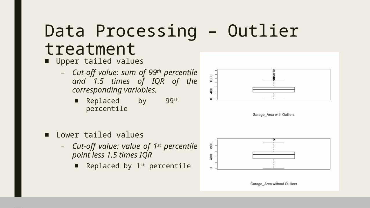
Data Processing – Outlier treatment■ Upper tailed values

– Cut-off value: sum of 99th percentile and 1.5 times of IQR of the corresponding variables.■ Replaced by 99th percentile

■ Lower tailed values– Cut-off value: value of 1st percentile

point less 1.5 times IQR■ Replaced by 1st percentile

Data Processing – Variable creation■ Character Variables

– (n – 1) indicators are created for a character variable containing n different categories

– Separate indicator created for missing value

■ Additional Indicator Variables– Based on bivariate plots: if two or more

categories contains similar level of value of dependent variable, they are combined and converted into an indicator

■ For example, Alley has three levels: Grvl, Missing and Pave. A new variable was created for Missing and Pave category as they both have a high median value of the dependent variable.

Method of Analysis■ Variable Selection Using Random Forest

■ Multiple Linear Regression– Significance

■ t value and probability of t value– Goodness of fit

■ Adjusted R-square– Multicollinearity

■ Random Forest

■ Model Accuracy– Error rate– MAPE

Introduction – Random Forest• Random Forest operate by constructing multitude of

decision trees at training time and outputting the mean prediction of the individual trees. It also correct the decision trees’ habit of over fitting to the training set.

• It is also been used to rank the importance of variables in a regression problem in a natural way.

• In a regression tree, for each independent variable, the data is split at several split points. Sum of Squared Error(SSE) at each split point between the predicted value and the actual values is calculated. The variable resulting in minimum SSE is selected for the node. Then this process is recursively continued till the entire data is covered.

Method of Analysis – Variable Selection■ Random Forest Model

– Model■ A model has been built on train data using

random forest – number of trees:100– Importance of Variables

■ Importance of Variables were extracted■ Variables are sorted descending based on

the importance measure– Variables selected in order of importance

measure are introduced into the OLS model Introduce one-by-one variable into model 2

Variables sorted in descending order of their importance

Table of variable importance

Model1- Random Forest

Method of Analysis – Multiple Linear Regression■ Ordinary Least Square (OLS) :

– Simplest method regression in which the unknown coefficients of features are estimated with the goal to minimize the sum square errors. i.e.

– Visually this is seen as the sum of the vertical distances between each data point in the set and the corresponding point on the regression line

Method of Analysis – Multiple Linear Regression■ Iteration

– Select one variable at a time from the variable importance table created using random forest

■ Significance– Check significance of new variable along with existing variables by its t-value and probability of t-statistics.– If R-square is improved, keep the variable, else drop it

■ Multicollinearity– Multicollinearity is checked at each step – ensuring the maximum value is < 4– If new variable has multicollinearity above threshold value – drop it– If introducing the new variable increases the multicollinearity of any existing variable – then the variable with

lowest t-value is dropped

■ Model Accuracy

– After adding the new variable, the model accuracy on train and test data using error rate and MAPE is checked.

– Drop the new variable if the model accuracy falls.

Method of Analysis – Random Forest• Variables• Using the same variable used in the linear regression

• Trees and Nodes• Checking various combinations of number of trees and maximum number of nodes to get the best

result.• Using number of trees = 100 and maximum nodes = 10 for best fitted model.

• Model Accuracy• Checking model accuracy using error rate and MAPE

• Decision • Drop the variable if the model accuracy falls or remains same.

Method of Analysis – Model Accuracy• Error rate• Calculated as : • Calculated minimum error rate and maximum error rate for train and test data.• Aim is to reduce the error rate • Difference between minimum and maximum error rate between training and validation.

• MAPE• Mean Absolute Percentage Error is calculated by :

• Aim is to minimize the MAPE

Results

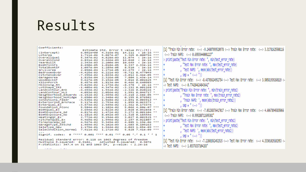
Result – Interpretation

■ Linear Regression Model– All the variables taken in the final

model.– Adjusted R-square is: 90.76

■ i.e. these variables together are explaining 90.76% variability of SalePrice.

– All of the variables are significant.– Multicollinearity is not severe. All

VIFs’ are below 4.

Result – Interpretation ■ Linear Regression Model

– Train Data■ Minimum error rate is -9.3%■ Maximum error rate is 3.35%■ MAPE is 0.697

– Test Data■ Minimum error rate is -8.68%■ Maximum error rate is 3.41%■ MAPE is 0.778

■ Random Forest Model– Train Data

■ Minimum error rate is -6.9%■ Maximum error rate is 4.49%■ MAPE is 0.993

– Test Data■ Minimum error rate is -7.29%■ Maximum error rate is 3.37%■ MAPE is 1.02

Result■ MAPE

– Low for Linear Regression – High for Random Forest

■ Linear Regression Model Chosen – based on minimum MAPE

THANK YOU

APPENDIX

Sample Predicted Sale Price – Linear Regression Model

Id SalePrice Id SalePrice Id SalePrice Id1461 126701.3 1483 175239.3 1505 225337.5 15271462 162982.1 1484 170172.4 1506 194180.3 15281463 178089.9 1485 175177.9 1507 271850.8 15291464 208902.2 1486 199074.1 1508 208083.3 15301465 193823.7 1487 309688.9 1509 159138.8 15311466 168862.5 1488 245865.5 1510 139717.4 15321467 193708.7 1489 190057.9 1511 151421.5 15331468 165445.6 1490 225320 1512 174073.1 15341469 196142.3 1491 193731.9 1513 138853.8 1535