High Performance Simulation for ATM Network Development

Final Study Report

for

New Zealand TeleCom

John Cleary

Murray Pearson

Ian Graham

Brian Unger

Department of Computer Science

University of Waikato

Abstract

Techniques for measuring and modeling ATM traffic a re reviewed.The requirements for cell level ATM network modeling and simulationare then outlined followed by a description of a n ATM traffic andnetwork (ATM-TN) simulator. This ATM-TN simulator is built uponparallel simulation mechanisms to achieve the high performanceneeded to execute the huge number of cell events required for arealistic network scenario. Results for several simulation experimentsare reported using this high performance simulator includingscenarios for the Wnet and OPERA networks. Finally, a preliminaryevaluation of the application of high performance simulation to thedesign and analysis of ATM network performance is provided.

June 1996

Table of Contents

1. INTRODUCTION 1

2. ATM NETWORK SIMULATION REQUIREMENTS 1

2.1 ATM Traffic Modeling 1

2.2 ATM Switch & Network Modeling 2

2.3 Simulator Performance 3

2.4 Production versus Research Issues 3

3. AN ATM TRAFFIC AND NETWORK SIMULATO R : ATM-TN 4

3.1 Support for Parallel Execution 4

3.2 Major Components & Interfaces 4

3.3 The ATM Modeling Framework 5

3.4 Traffic Models 6

3.5 Switch Models 8

4. A HIGH PERFORMANCE SIMULATION ENVIRONMEN T : SIMKIT 1 0

4.1 Background 1 0

4.2 Logical Process Modeling Methodology 1 1

4.3 Design Philosophy 1 2

4.4 Programming Model 1 4

4.5 Time Warp Constraints 1 5

4.6 Run Time Configuration 1 5

5. PRELIMINARY EXPERIMENTS USING THE ATM-TN 1 6

5.1 A Western Canadian (Wnet) Experiment 1 6

5.2 Telecom New Zealand’s OPERA Experiments 2 1

6. PERFORMANCE OF THE ATM-TN SIMULATOR 2 8

7. CONCLUSIONS 2 9

APPENDIX A : CELL LEVEL MEASUREMENTS OF ATM-25 TRAFFIC

APPENDIX B : CONSERVATIVE PARALLEL SIMULATION OF ATMNETWORKS

iii

List of FiguresFIGURE 1 ATM-TN SIMULATOR ARCHITECTURE 5FIGURE 2 THE WNET ATM NETWORK 17FIGURE 3 UTILIZATION OF LINK 15 21FIGURE 4 AVERAGE CELL DELAY FOR THE JPEG1 LOAD 21FIGURE 5 CELL DELAY VARIATION 21FIGURE 6 BUFFER OCCUPANCY FOR THE CALGARY_AGT SWITCH 21FIGURE 7 THE TELECOM NEW ZEALAND OPERA NETWORK 22FIGURE 8 NETWORK CONNECTIONS AND LINKS 23FIGURE 9 AVERAGE MPEG CELL DELAY 24FIGURE 10 STANDARD DEVIATION OF MPEG CELL DELAY 24FIGURE 11 AVERAGE ETHERNET CELL DELAY (ALBANY TO DUNEDIN) 25FIGURE 12 STANDARD DEVIATION OF ETHERNET CELL DELAY (ALBANY TO DUNEDIN) 25FIGURE 13 AVERAGE CELL DELAY (ALBANY - WAIKATO) 25FIGURE 14 STANDARD DEVIATION OF CELL DELAY (ALBANY - WAIKATO) 25FIGURE 15 BUFFER OCCUPANCY AT PALMERSTON NORTH PORT OF WAIKATO SWITCH 26FIGURE 16 BUFFER OCCUPANCY AT PALMERSTON NORTH PORT OF WAIKATO SWITCH 26FIGURE 17 ALBANY - WAIKATO LINK UTILIZATION 26FIGURE 18 ALBANY - WAIKATO LINK UTILIZATION 26FIGURE 19 CELLS DROPPED ON THE ALBANY - WAIKATO LINK 27FIGURE 20 PRELIMINARY SIMULATOR PERFORMANCE FOR THE WNET SCENARIO 28

List of TablesTABLE 1 ESTIMATED WNET USER BANDWIDTH & QOS REQUIREMENTS 17TABLE 2 SIMULATED QOS RESULTS FOR BENCHMARK 1 18TABLE 3 SIMULATION UTILIZATION RESULTS FOR BENCHMARK 1 18TABLE 4 QUALITY OF SERVICE RESULTS FOR BENCHMARK 2 19TABLE 5 QUALITY OF SERVICE RESULTS FOR BENCHMARK 3 19TABLE 6 UTILIZATION RESULTS FOR BENCHMARK 3 19TABLE 7 CELL DELAY FOR EACH TRAFFIC SOURCE AND SINK STREAM 27

1. Introduction

This report summarizes research that has been aimed at the measurement andcharacterization of ATM multimedia traffic, the modeling and simulation ofATM networks, and the design of high performance simulation engines that arecapable of supporting very computation intensive ATM network simulations.The results of work performed at Waikato as part of this study for TeleCom isincluded along with closely related work that has been completed elsewhere.

First, the requirements of a cell level ATM network simulator are outlined insection 2.0. This involves traffic characterisation, ATM switch modeling, andnetwork level modeling. Next, the architecture and major components of anATM traffic and network (called the ATM-TN) simulator are presented in 3.0. Ahigh performance simulation environment on which the ATM-TN simulator isbased is then described in section 4.0. In section 5.0, simulation results for severalATM network scenarios, including one for OPERA, are outlined. Section 6.0presents a preliminary evaluation of high performance simulation as amethodology for the analysis and design of ATM networks. Conclusions areoutlined in section 7.0

The body of this report represents a brief overview of the work accomplished. Adetailed review of techniques for the measurement and modeling of ATM celllevel traffic is presented in a companion paper [Pearson et. al. 96]. Measurementresults for a specific multimedia scenario are included in Appendix A.Preliminary work on a next generation high performance simulation engine iscontained in Appendix B.

2. ATM Network Simulation Requirements

The general requirements of an ATM network simulator are to support: networkperformance analysis under varying traffic types and loads, network capacityplanning, traffic aggregation studies, and ATM network protocol research. Thisspans a wide range of applications from production use by ATM networkplanners to ATM switch, network and protocol design by researchers.

These general requirements imply the need for cell level models of arbitrarynetwork topologies with tens to hundreds of switches; models of multiple switcharchitectures and the characterisation of a range of ATM network traffic sources.The requirements of the traffic models, switch and network models, simulatorrun-time performance, and other simulator requirements are outlined in thisreport. These model components are all part of a modeling environment calledthe ATM-TN.

2.1 ATM Traffic Modeling

Three basic types of network traffic models are required in a general ATMnetwork modeling environment: both compressed and uncompressed videotraffic, an Internet traffic model of World Wide Web (WWW) browsinginteractions, and aggregate ethernet local area network (LAN) traffic. Specifically,each of the ATM-TN traffic models should support:

• point to point traffic definitions for multiple traffic types and varyingtraffic rates;

• dynamic bandwidth allocation and deallocation;

• statistics for cell loss ratios (CLR), cell transfer delay (CTD) and cell delayvariation (CDV); and

• higher level traffic protocols and statistics specific to traffic types, eg.,TCP/IP packet level statistics such as error rates, packet sizes and delays.

All of the traffic models should capture the behavior of different types of userdemands for communication services. Each type of traffic model will ultimatelygenerate ATM cells as input to the network.

In the future, other traffic models in addition to the above will need to beincorporated. Modeling specific TCP/IP applications and LAN-ATM-LAN trafficincluding the (ATM Adaptation Layer) AAL functions are examples ofanticipated future requirements.

2.2 ATM Switch & Network Modeling

The ATM-TN will model the protocols for ATM switching, call setup andrelease, and parts of the ATM Adaptation Layer (AAL). Other protocols such aspolicing and admission control will need to be modeled in the future. The latterwill require the ATM-TN core models to be extensible.

The switch models must characterise the flow of ATM cells through the networkas determined by the specific architecture of each switch type. The followingoutlines some of the elements that must be represented. Each type must bemodeled using sub-components:

• a dimension (NxN) specifying the number of input ports and outputports on the switch;

• a switching fabric, defining the connections between input ports andoutput ports (eg., crossbar, shared bus, banyan, delta network, ...);

• a set of buffers and a buffering strategy that specifies how many buffersare available, and how they are configured and used (eg., shared vs.partitioned, input vs. output buffering); and

• routing tables, used to map cells from input ports to output ports. Thismapping is done using virtual circuit and virtual path indices (VCIsand VPIs).

Links (or ports) must be modeled implicitly in the exchange of cells betweenswitches (eg., capacity in bits/sec, propagation delay, and bit error rate) rather thanexplicitly as a separate model component. This approach will significantly reducethe number of simulation events.

The intent is to make it easy to "plug and play" to evaluate the performanceimplications of different ATM switch architectures, and later, of different switchcall admission, policing, and traffic control mechanisms.

2.3 Simulator Performance

The applications of the ATM-TN will require simulations of between 109 and 1012

cells. In a straightforward characterisation of cell interactions through networkswitches this implies roughly five to ten times that number of simulationevents.

Desirable simulation run-times are less than two hours with a maximum of 12hours for overnight execution. These execution times are clearly not feasible forsimulations of more than about 109 cells. Thus, extraordinary approaches will berequired to achieve reasonable simulation run-times.

Initially it is not desirable to introduce approximations or hybrid analytic andsimulation approaches. It is important that a high fidelity, accurate, model bedeveloped first which can be used to validate simulator optimizations, and thenapproximate and hybrid approaches. Thus, despite the run-time requirements,an initial ATM-TN version is required that is capable of closely mimicking actualtraffic and network behavior. Further, it is desirable that test and debug runs canbe executed on ubiquitous PCs and Unix workstations.

In summary, the simulator efficiency will be crucial and care is needed to createvery efficient sequential and parallel kernels.

2.4 Production versus Research Issues

A significant part of the ATM-TN simulator requirements are to support“production” ATM network sizing and planning by network planners. Thisrequires a non-programmer interface that offers interactive data managementand experiment control tools for large input and output files. The input filesinclude an array of parameters to define specific switch and link characteristics, todefine network configurations, and to specify experiment scenarios. Output filesshould be structured to enable the use of third party spreadsheet, statistical andgraphical data analysis tools.

The other major goals of an ATM-TN simulator are to support research. Thecurrent ATM networking research issues of interest include: call admissioncontrol on entrance to the network, congestion control within the network,usage parameter control (UPC) within the network and switch service disciplines(scheduling policies). Other issues alluded to in the above sections include:multicast routing, switch architectures within network context and networkmanagement protocols.

Finally, there are research issues in modeling and simulation methodologies forthis application. These include workload and traffic characterisation in terms ofmeasurable parameters, the design of efficient simulation kernels, hybridanalytic and simulation approaches, and the parallel execution of ATM trafficand network models. The requirements of an ATM-TN include being able toaddress these simulation methodology issues, the open issues in ATMnetworking outlined above, as well as, the commercially important networkplanning issues.

3. An ATM Traffic and Network Simulator : ATM-TN

The ATM-TN simulator presented here was designed to meet all of therequirements outlined in section 2. The main design principles were to: (1)accurately mimic ATM network behavior at the cell level for specifiable trafficloads, (2) create a modular extensible architecture since requirements will evolveas new issues emerge, (3) achieve reasonable execution times for ATM networksthat consist of hundreds of nodes and thousands of traffic sources. Since (1)implies an extremely computationally intense simulator and (2) implies a longlived simulator it is reasonable to expend substantial effort on (3). Further detailson the ATM-TN can be found in Gburzynski (1995).

3.1 Support for Parallel Execution

A cell level simulator for a moderately large ATM network has substantialpotential for parallel execution. There is a great deal of independent activityinvolved in a large number of individual streams of cells flowing through alarge network. Our analysis of the run-time behavior of an ATM-TN and relatednetwork simulation problems [Unger et al. 94a, Unger & Xiao 94b, Unger &Cleary 93] suggests that optimistic synchronization schemes have potential.

Although a decade of research in optimistic synchronization methods forachieving speedup through parallel execution on multiprocessor platforms hasstill produced mixed results, it was decided that the emergence of moderatelylarge shared memory multiprocessor systems would have much greater potentialfor speedup in an ATM-TN simulator [Unger et al. 93]. This led to the design anddevelopment of SimKit and WarpKit [Gomes et al. 95].

Simulations written in SimKit can be executed either sequentially or in parallel.The optimized sequential simulator (OSS) has been developed to support veryfast, efficient, sequential execution. The second kernel, called WarpKit, supportsparallel execution on shared memory multiprocessor platforms based on theVirtual Time (Time Warp) paradigm defined in [Jefferson 85 and Fujimoto 90b].

The WarpKit kernel design is based on research reported in [Fujimoto 90a,Baezner et al. 94 and Unger et al. 90]. The design of both WarpKit and SimKit areaimed at general purpose discrete event simulation problems. However, SimKit(see section 5) enables building custom mechanisms to support very efficientconstructs that appear frequently in the implementation of network simulators,or specifically, in the ATM-TN.

3.2 Major Components & Interfaces

The general structure of the ATM-TN simulator is illustrated in Figure 1. Themajor components include: traffic models, switch models, an ATM ModelingFramework, SimKit, WarpKit, OSS and the TeleCom Modeling Framework(TMF). The TMF and ATM Modeling Framework are outlined below. The trafficand switch models are described in subsequent sections.

The TMF enables the TeleCom engineer to configure a specific simulation modeland vary model component parameters. The user constructs a model byspecifying network topology, switch architectures, the traffic sources and the links

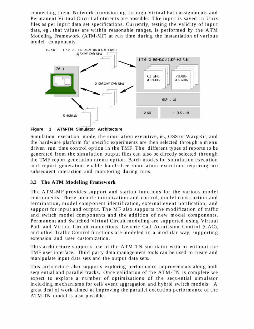
connecting them. Network provisioning through Virtual Path assignments andPermanent Virtual Circuit allotments are possible. The input is saved in Unixfiles as per input data set specifications. Currently, testing the validity of inputdata, eg., that values are within reasonable ranges, is performed by the ATMModeling Framework (ATM-MF) at run time during the instantiation of variousmodel components.

Figure 1 ATM-TN Simulator Architecture

Simulation execution mode, the simulation executive, ie., OSS or WarpKit, andthe hardware platform for specific experiments are then selected through a menudriven run time control option in the TMF. The different types of reports to begenerated from the simulation output files can also be directly selected throughthe TMF report generation menu option. Batch modes for simulation executionand report generation enable hands-free simulation execution requiring nosubsequent interaction and monitoring during runs.

3.3 The ATM Modeling Framework

The ATM-MF provides support and startup functions for the various modelcomponents. These include initialization and control, model construction andtermination, model component identification, external event notification, andsupport for input and output. The MF also supports the modification of trafficand switch model components and the addition of new model components.Permanent and Switched Virtual Circuit modeling are supported using VirtualPath and Virtual Circuit connections. Generic Call Admission Control (CAC),and other Traffic Control functions are modeled in a modular way, supportingextension and user customization.

This architecture supports use of the ATM-TN simulator with or without theTMF user interface. Third party data management tools can be used to create andmanipulate input data sets and the output data sets.

This architecture also supports exploring performance improvements along bothsequential and parallel tracks. Once validation of the ATM-TN is complete weexpect to explore a number of optimizations of the sequential simulatorincluding mechanisms for cell/event aggregation and hybrid switch models. Agreat deal of work aimed at improving the parallel execution performance of theATM-TN model is also possible.

Figu re 1 ATM-TN Simulato r A rch ite cture

Output Data Set

TMF

ATM Modeling Framework

TrafficModelsTraffi c

ModelsTrafficModelsSwitchModels

TrafficModelsTraffic

ModelsTrafficModel sTraffic

Models

SimKit

WarpKitOSSReports

Inpu t Data Set

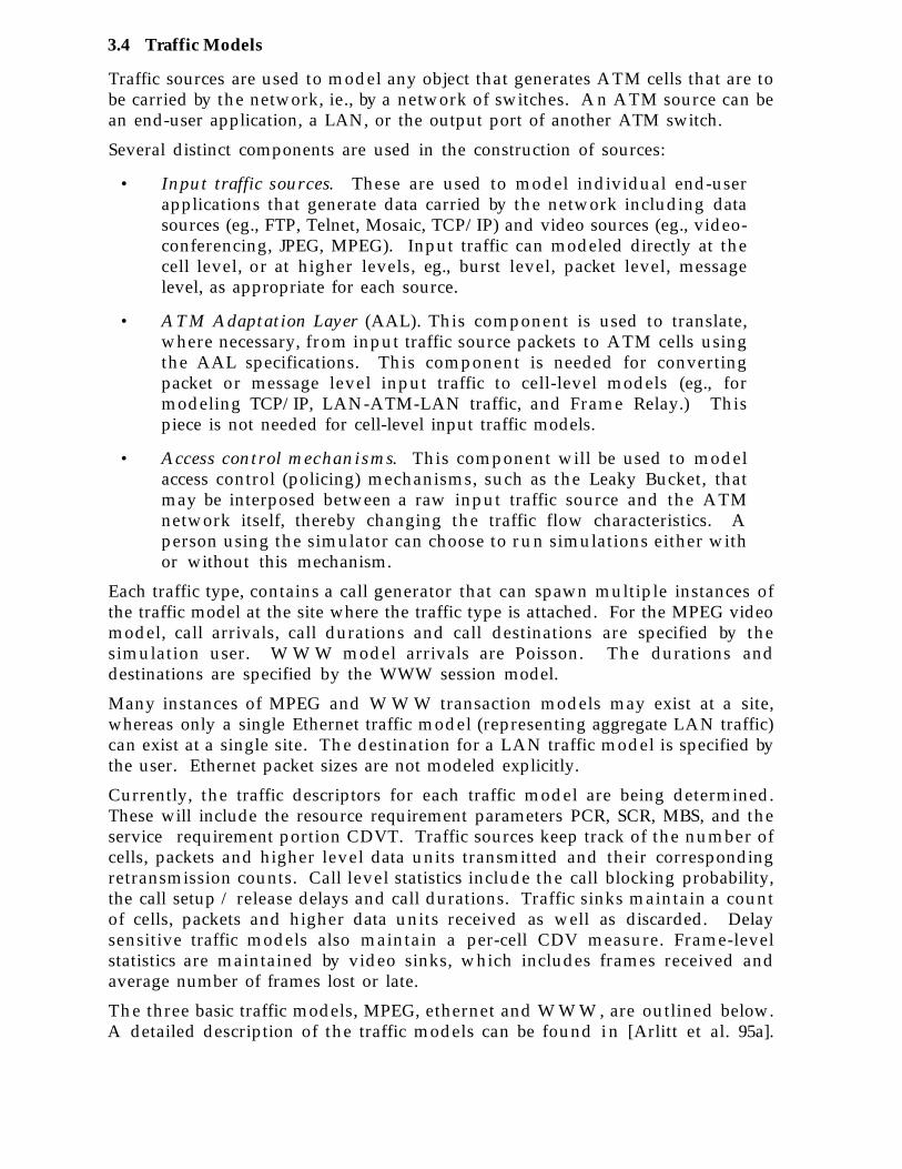
3.4 Traffic Models

Traffic sources are used to model any object that generates ATM cells that are tobe carried by the network, ie., by a network of switches. An ATM source can bean end-user application, a LAN, or the output port of another ATM switch.

Several distinct components are used in the construction of sources:

• Input traffic sources. These are used to model individual end-userapplications that generate data carried by the network including datasources (eg., FTP, Telnet, Mosaic, TCP/IP) and video sources (eg., video-conferencing, JPEG, MPEG). Input traffic can modeled directly at thecell level, or at higher levels, eg., burst level, packet level, messagelevel, as appropriate for each source.

• ATM Adaptation Layer (AAL). This component is used to translate,where necessary, from input traffic source packets to ATM cells usingthe AAL specifications. This component is needed for convertingpacket or message level input traffic to cell-level models (eg., formodeling TCP/IP, LAN-ATM-LAN traffic, and Frame Relay.) Thispiece is not needed for cell-level input traffic models.

• Access control mechanisms. This component will be used to modelaccess control (policing) mechanisms, such as the Leaky Bucket, thatmay be interposed between a raw input traffic source and the ATMnetwork itself, thereby changing the traffic flow characteristics. Aperson using the simulator can choose to run simulations either withor without this mechanism.

Each traffic type, contains a call generator that can spawn multiple instances ofthe traffic model at the site where the traffic type is attached. For the MPEG videomodel, call arrivals, call durations and call destinations are specified by thesimulation user. W WW model arrivals are Poisson. The durations anddestinations are specified by the WWW session model.

Many instances of MPEG and WWW transaction models may exist at a site,whereas only a single Ethernet traffic model (representing aggregate LAN traffic)can exist at a single site. The destination for a LAN traffic model is specified bythe user. Ethernet packet sizes are not modeled explicitly.

Currently, the traffic descriptors for each traffic model are being determined.These will include the resource requirement parameters PCR, SCR, MBS, and theservice requirement portion CDVT. Traffic sources keep track of the number ofcells, packets and higher level data units transmitted and their correspondingretransmission counts. Call level statistics include the call blocking probability,the call setup / release delays and call durations. Traffic sinks maintain a countof cells, packets and higher data units received as well as discarded. Delaysensitive traffic models also maintain a per-cell CDV measure. Frame-levelstatistics are maintained by video sinks, which includes frames received andaverage number of frames lost or late.

The three basic traffic models, MPEG, ethernet and WWW, are outlined below.A detailed description of the traffic models can be found in [Arlitt et al. 95a].

Further information on the WWW model is presented in [Arlitt & Williamson95b] and on the ethernet model in [Chen et al. 95].

3.4.1 MPEG and JPEG Video Models

The MPEG/JPEG video traffic model is designed to characterise theunidirectional transmission of a single variable bit rate compressed video streamof data. This video data is both delay-sensitive and loss-sensitive; if cells are lost,image quality is degraded, and if cells arrive late, they are discarded, ie., the effectof delay can be the same as if they were lost.

The MPEG (motion pictures expert group) algorithm is a standardized method ofcompressing full motion video for storage as digital data. An MPEG videostream consists of a sequence of images, or frames, that are displayed one after theother at short periodic intervals. The standard defines three types of three typesof compressed frames called I, P and B frames as follows:

• I frames are encoded using only the image data available within thecurrent frame. Thus an I (intraframe) frame represents a completeimage, they provide an absolute reference point for the other twoimage types in an MPEG sequence.

• P frames contain motion-compensated data predicted from thepreceding I or P frame. P (predicted) frames take longer to encode thanI frames, are faster to decode than I frames, and achieve highercompression than I frames.

• B frames contain motion-compensated data from both the previousand the next frame (I or P). B (bi-directional interpolative) frames takethe longest time to encode but offer the greatest compression.

A JPEG stream consists of all I frames and thus provides compression on eachframe as an independent unit of data. MPEG sequences consist of a pattern of I,Pand B frames called a group of pictures (GOP). The GOP frame is specified at thestart of encoding, eg., an IBBPBBPBBI sequence which is continually repeated.

The MPEG video traffic model in the ATM-TN simulates cell level ATM trafficgenerated by an MPEG video stream to a viewer. The model generates a givencombination of I, P and B frames at a set frame rate. These random sequences aregenerated using the transform-expand-sample (TES) modeling methodologydefined by [Melamed and Hill 95]. Here, TES is used to generate threeautocorrelated sequences of frame sizes, one for each type of MPEG frame. Theseseparate sequences are then interleaved according to the GOP to produce thesimulated traffic. Thus, this MPEG/JPEG traffic model is a composite TES model.

3.4.2 An Aggregate Ethernet Model

The ethernet LAN model is designed to represent aggregate data packet traffic onexisting local area networks such as a university campus LAN. One of therequirements of the ATM-TN is to characterise ATM connections between legacyLAN networks as part of the evolution to ATM. This kind of traffic is likely toform a significant fraction of background load for early configurations of ATMnetworks.

Recent research confirms that ethernet traffic exhibits a fractal, self-similar,behavior where there is no natural length for bursts. This means that Poissonmodels do a very poor job of representing ethernet traffic. A stochastic process issaid to be self-similar with Hurst parameter H if the process is covariancestationary and aggregate versions of the same process have the same structure asthe original process. Thus, bursts are visible in aggregated traffic on a wide rangeof time scales, eg., from milliseconds to minutes.

This self similar behavior has been observed both in traffic internal to anethernet LAN, as well as, to traffic leaving a LAN. This behavior has beenobserved by researchers at Bellcore, and we have observed similar behavior inmeasurements taken at the University of Saskatchewan. The latter suggest self-similar behavior with a Hurst parameter close to 0.7. The ATM-TN aggregateethernet traffic model is based on the TES methodology for generating randomtraffic sequences that have validated first and second order time series statistics,ie., a frequency histogram and autocorrelation function that matches actual LANmeasurement data.

3.4.3 A World Wide Web Transaction Model

The ATM-TN WWW model characterizes the cell traffic generated during aMosaic like browser session exploring WWW servers. A single Mosaic sessioncan generate one or more Mosaic conversations. Multiple destination sites maybe involved in a single session, one destination at a time. Each conversationmay consist of one or more TCP connections. Each TCP connection represents asingle VC connection requiring an independent connection setup. A WWWsession can spawn multiple conversations, eg., from one to hundreds, and eachconversation can spawn multiple connections, eg., one to ten connections.

The input parameters to a WWW session include: mean number ofconversations per session (Geometric distribution), mean conversation gap time(Poisson model), conversation destination, mean number of connections perconversation (geometric), mean connection gap times (Poisson) and the amountof information exchanged during a connection. In the latter, bytes sent by thesource are modeled using a log Normal distribution, bytes received from thedestination are modeled using a log Erlang distribution, and the mean andstandard deviations are input parameters.

A single WWW session may last minutes or hours representing a user searchingfor information across the Internet. Empirical measurements of Internet WWWtraffic collected at the University of Saskatchewan were used to construct andparameterize this model. Traces were collected using the Unix tcpdump andthousands of TCP connections were observed. Four one day traces were collectedwhich contained 5,829 conversations which formed 57% of the total networkactivity.

3.5 Switch Models

The ATM-TN switch models currently include three simple, and threemultistage switch models. These models support point-to-point switched virtualchannels (SVCs) and permanent virtual channels (PVCs). The SVC call setupand release procedures modeled closely approximate the UNI 3.0 specification

[ATM 93]. Virtual Paths (VPs) are also characterized and defined by input data asthey tend to be long lived connections.

An ATM-TN network model has a number of components including:communication links, traffic source / sinks (TSSs), end nodes and switches. Endnodes are a simplified type of switch that is used at the edges of an ATM network.The switch models provide:

• a simple traffic shaping scheme on a per VC basis,

• a simple call admission control (CAC) scheme at each switch,

• a user parameter control (UPC) scheme at each UNI access switch,

• a network parameter control (NPC) scheme per NNI (internal switch),

• separate buffer queues for the CBS/VBR/ABR/UBR service categoriesand a mechanism for scheduling the removal of cells from thesequeues. This is done at every output port, and

• separate thresholds for dropping cells with high loss priority and forforward loss congestion notification.

The basic operation of an ATM switch model is relatively simple. A cell thatarrives on input port i with VCI=m and VPI=n is looked up in the routing table,and mapped to output port j with VCI=p and VPI=q. Real switches must be ableto do this many thousands of times per second (eg., 53-bytes @ 150 Mbps = 2.83usec/cell). The VCI/VPI mappings are determined at the time of call setup usingan in-band signaling protocol.

The switch models also handle signaling for call setup and release which makesthese models much more complex. VCIs are dynamic ie., they are allocated anddeallocated on a millisecond-second-minute time scale, while VPIs will be fairlystatic, ie., they are allocated and deallocated on an hour-week-month time scale.

3.5.1 ATM Signaling

The model of signaling is one of the more complicated parts of the ATM-TN.However, signaling needs to be characterized since the overhead of end-to-endconnection setup becomes significant as network speed increases. The modelattempts to closely represent the UNI 3.0 specification [ATM 1993].

The model of network functions within switches follows the standard ATMlayering, ie., the network layer where the signaling protocol is implemented, theapplication layer at the end nodes which provide the interface to the trafficmodels, the signaling ATM adaptation layer which implements segmentationand reassembly, and the ATM layer which manages cell level transactions, are allcharacterized.

The signaling layer implements ATM connections, and thus the call setup andcall release functions. Basic call admission and bandwidth allocation functionsare represented. VP, VC, PVC and SVC connections are supported in the switchmodels.

3.5.2 Switch Model Architecture

The basic switch models have two major components, the control module andthe switch fabric. When signaling cells arrive at a switch they are routed to theinternal control module. The control module implements the signalingfunctions by acting on the information carried in these cells and sends outadditional signaling cells of its own. This module also makes call admission androuting decisions, and updates the VPI/VCI translation tables within the switch.

The switch fabric transfers cells from an input port to the appropriate output portor to the control module. The switch buffering strategy is implemented in thefabric, eg., output buffering, shared memory buffers, or a crossbar architecture.Multistage switches can be constructed from one of the basic switch types. Mostlarger switches contain banyon fabrics that can be scaled up to m any thousandsof ports. A more complete description of the ATM-TN switch and signalingmodels is presented in [Gburzynski et al. 95].

4. A High Performance Simulation Environment : SimKit

SimKit is a C++ class library that is designed for very fast discrete eventsimulation. SimKit presents a simple, elegant Logical Process View ofsimulation enabling both sequential and parallel execution without code changesto application models. The sequential executive performs well on a variety ofUNIX platforms and facilitates debugging and testing. The current parallelexecutive (WarpKit) is based on the Time Warp paradigm and supports efficientparallel execution on shared memory multiprocessor hardware such as theSilicon Graphics Power Challenge and the Sun SparcServer 1000/2000. A second“conservatively” synchronized parallel executive that is under development ispresented in Appendix B.

This section describes the design features of the SimKit System. A brief overviewof the Logical Process Modeling View commonly used in Parallel Discrete EventSimulation (PDES) is presented. The SimKit classes are then introducedfollowed by a brief description of how to build and simulate object orientedmodels using SimKit.

4.1 Background

The suitability of simulation as a tool to analyze large, complex broadbandcommunication systems depends on very high speed execution. Typical ATMnetwork simulations may require simulating 109 to 1012 events which at a rate ofone event per 50 microseconds requires an execution time of 15 to 1,500 hours.This gives a strong motivation for exploring PDES methods to decreasesimulation time by parallel execution.

PDES systems, in general, eliminate the globally shared event list and resort to asynchronization protocol to insure causality between events being executed inthe parallel system. The principle distinguishing features of the synchronizationapproach are the degree of aggressiveness and the risk employed.Synchronization algorithms have been broadly classified as Conservative orOptimistic [Reynolds 88]. The Time Warp mechanism is a well known optimisticapproach based upon the Virtual Time paradigm [Jefferson 85]. Time Warp,

essentially non blocking, does not strictly adhere to the local causality constraint.It relies upon a causality error detection and recovery scheme based on a rollbacktechnique.

In the last fifteen years, research in PDES [Fujimoto and Nicol 92, Ferscha andTripathi 94] have primarily focused on attainable simulation execution speedups.The main reason why PDES has not yet been embraced by the generalcommunity is the lack of research contributions toward simplifying thedevelopment of simulation models for concurrent execution [Page and Nance 94,Unger and Cleary 93]. Simulation modeling for parallel execution can be a verypainstaking process.

PDES assumes a Logical Process Modeling methodology for simulation softwaredevelopment. The system to be simulated is conceptualized as a network ofinteracting physical sub-systems [Chandy and Misra 79 and 81]. The physicalconcurrency in these sub-systems translates into computational concurrency inthe simulation, which may be utilized through parallel execution. The lack of aglobal event list, constraints of the synchronization algorithm and the incidentallogical process view of modeling make the design of a parallel simulationlanguage difficult. The language should provide a rich set of primitives thatfacilitate model expression and simulation transparently of the underlyingsynchronization mechanism while at the same time allowing maximumparallelism to be extracted from the model.

SimKit is a C++ class library that is designed for very fast discrete eventsimulation. SimKit presents a simple logical process view of simulationenabling both sequential and parallel execution without code changes to theapplication models. A brief overview of logical process modeling methodologyinnate within PDES is presented in section 5.2. Section 5.3 lists the issues thatdictate parallel simulation language design considerations. The designphilosophy adopted in the SimKit System is then outlined followed by thefeatures of the SimKit System.

4.2 Logical Process Modeling Methodology

In PDES, the physical system to be modeled is conceptualized as a system ofinteracting physical processes (PPs). A distributed simulation model of thephysical system is represented by a topologically equivalent system ofcomputational units called logical processes (LPs). Each LP is responsible forsimulating events in a sub-space modeling the activities occurring in thecorresponding PP. The interaction between PPs is modeled by the correspondingLPs communicating via timestamped messages. The timestamp represents theevent occurrence time in the simulation. State transitions in the physical systemare modeled by the occurrence of an event, ie., the receipt of a timestampmessage at the destination LP. Occurrence of an event may involvemodifications to the state and/or the causing of new events in the future.

Distributed simulation accelerates the execution of the program by executing thecomputational units (LPs) concurrently on multiple processors. By nature, in adistributed simulation system, there is no notion of a global clock or a centralevent list. LPs execute in parallel by maintaining their own local clock and eventlist. A synchronization algorithm is used to insure that the local causality

constraint is maintained at each LP. In this logical process modelingmethodology the sharing of state between LPs is not possible.

4.3 Design Philosophy

A plethora of parallel simulation languages have appeared in the last decade,each with differing design considerations. These languages include: CommonInterface of OLPS [Abrams 88 and 89], Maisie [Bagrodia and Liao 90], ModSim[West and Mullarney 88, Rich and Michelsen 91], MOOSE [Waldorf and Bagrodia94], SCE from MITRE [Gill et. al. 89], Sim++ from Jade [Baezner, Lomow andUnger 90 and 94], SIMA [Hassam 91], RISE from RAND [Marti 88] and Yaddes[Preiss 89]. The major differences between these languages are their approach to:

• programming paradigm employed and language constructs,

• underlying synchronization protocol and transparency,

• modeling world view,

• run time configuration,

• determinism, and

• efficiency.

The desired characteristics of a parallel simulation language [Abrams and Lomow90] include: simplicity, modularity, portability, transparency, evolvability,efficiency, scalability, determinism, and generality. "The primary goal of theSimKit System was to provide an event-oriented logical process modelinginterface that facilitates building application models for sequential and parallelsimulation with high performance execution capabilities."

The design philosophy of the SimKit interface can be summarized as:

• ease of use with the ability to reuse model components,

• indifference towards the underlying simulation control system,

• execution mode transparency,

• encompassing a wide range of applications and user base, and

• efficient event-oriented logical process paradigm,

Specific design features of the SimKit System include an object programmingmodel, transparency, evolvability and efficiency.

Object Oriented Programming Model

The SimKit library is implemented in the commonly-used general-purposeobject-oriented programming language, C++. Object oriented techniques allowfor reusable simulation models and software components to be developed. Theiterative nature of a simulation life cycle is well supported by the object-orientedparadigm. Object-oriented techniques along with good software engineeringprinciples can be used to design reliable simulation software, eg. scoping via

objects can be used to create complex simulations involving complex object classhierarchies.

By extending an existing language, the highly optimized library routines forparallel programming provided for a given architecture, can be directly used inthe implementation of the underlying synchronization scheme. Moreover, theavailability of debuggers, software engineering tools, etc. increase productivityand portability. Application programmers are not burdened with learning a newlanguage and can concentrate on the system modeling task. The SimKit Classlibrary includes only three classes, namely, "sk_simulation" for simulationcontrol, "sk_lp" for modeling application sub-space behavior and statetransitions, and "sk_event" to model the interaction between the logicalprocesses.

4.3.1 Transparency

The design of the Parallel SimKit system highlights the need for hiding issuespertaining to the underlying synchronization algorithm, wherever possible.Time Warp relies on a rollback mechanism, hence great care was taken inproviding primitives for error handling, output handling and dynamic memorymanagement. However, the application programmer is responsible to efficientlyuse the various state saving mechanisms provided. State Saving is an artefact ofthe need to support the rollback mechanism in Time Warp and for the present isleft under the jurisdiction of the application programmer as a trade off forefficiency. State restoration during rollback is transparent to the applicationprogram. SimKit libraries include a comprehensive set of pseudo-randomnumber distributions with efficient state saving of the seeds. LP allocation toprocessors in the parallel system is static and may be optionally specified by theprogrammer.

4.3.2 Evolvability

SimKit provides a general purpose simulation interface. Parallel SimKit hasbeen implemented on the WarpKit executive. Great care was taken toimplement a minimal clearly-defined interface to the WarpKit Kernel. Theinterface consists of three classes, namely, "wk_simulation", "wk_lp" and"wk_event". The SimKit classes (Parallel implementation) are derived fromthese mirror WarpKit classes. The Time Warp related quasi-operating systemservices like event-delivery, rollback, and commit are provided as virtualfunctions in the wk_lp class. This minimizes the impact of modifications to theunderlying synchronization system on the Programmer's Interface andconsequently the application itself. Evolving schemes and feature extensions canbe easily integrated into the simulation control engine without affecting theSimKit programmer's interface.

4.3.3 Efficiency

SimKit is a high performance language that presents an event-oriented logicalprocess view to the model developer. SimKit design goals are to supportefficient sequential and parallel execution without code changes to theapplication model. The sequential simulation control system is a highlyoptimized simulator that uses the splay tree implementation of the future event

list. The parallel simulation control system is capable of exploiting the inherentparallelism in applications having very low event computation granularities.

The parallel run time system, ie., WarpKit, consists of a variation of the TimeWarp protocol optimized for execution on shared memory multiprocessors. Theglobal control algorithms are asynchronous in nature, with minimal locking ofshared structures. The design of global control algorithms demonstrate a highdegree of scalability ie. minimal performance degradation with an increase in thenumber of processors used. The problem of state saving and restoration in TimeWarp is addressed by providing a grab bag of state handler objects that are finetuned for saving integers, floats, doubles, pointers, variable length state and blockstates incrementally.

The event-oriented view of simulation enables efficient scheduling of events viainvocation of the corresponding LP's event-processing member function ratherthan the costly context-switching approach in a process-oriented approach. Also,the memory requirements are lower as LP's are active only for the duration of anevent ie. no need for a stack per LP in the simulation.

The sequential executive performs well on a variety of platforms and facilitatesdebugging and testing. The per event scheduling overheads for the sequentialexecutive on an SGI Power Challenge, IRIX64 Release 6.0 IP21 MIPSmultiprocessor architecture using the ATT C++ compiler version 3.2.1 with the -O2 compiler option, is 2.2 microseconds. The per event overheads for the parallelexecutive is 8.6 microseconds.

4.4 Programming Model

The SimKit Programmer's Interface consists of three classes, one type and severalconvenience functions and macros. The three classes are: "sk_simulation","sk_lp", and "sk_event". The one type is "sk_time". Also a library for randomnumber generation and distributions is provided which includes classes foruniform, normal, exponential, geometric, binomial, Erlang and Poissondistributions.

The simulation model is constructed by deriving LPs from the sk_lp class andmessages (or events) from the sk_event class. The main function is in themodelers domain and may be used to incorporate third party tools like a lex/yaccprogram code to parse the simulation input parameters. The user instantiatesone instance of the sk_simulation class.

This object provides the initialization interface to the run time simulationkernel. The type sk_time is used to represent simulation time and supportsstandard arithmetic operators associated with the type double. The conveniencefunctions and macros are provided for easy access to simulation structures likecurrent LP, current event, and current time.

The modeler specifies an LP's activity via the sk_lp::process pure virtual memberfunction. The kernel delivers an event to a LP by invoking this function withthe event object as a parameter. Typically, the process function is coded as a largecase statement with the event type specifying the branching of control. Twoother virtual members provided are the sk_lp::initialize and the

sk_lp::terminate. These may be optionally defined to initialize the LP and fordoing wrap up LP work (eg. printing LP statistics and reports), respectively.

The derived message types may contain other application specific data (besidesevent type) that are communicated between the LP's. Alternatively, a messagemay be a query message to determine the value of another LP's state as no sharedvariables are allowed. A message is created using the SimKit overloaded event'sn e w operator. The sk_event::send_and_delete is the only eventsynchronization primitive that is necessary in this logical process view.

4.5 Time Warp Constraints

The following constraints extraneous to logical process modeling view are nativeto the parallel synchronization mechanism. Output handling and error handlingshould be rollback-able. Hence the modeler should use the member functionsprovided in the sk_lp class. General purpose memory management is anotherfacility that is provided via the sk_lp class. The request for dynamic memorydoes not return if the allocation request cannot be satisfied due to systemresource exhaustion. To support parallel simulation in particular, the simulationexecution phase has been divided into 6 clearly defined phases.

State Saving calls must be explicitly programmed with the LP's process function.A grab bag of state savers are provided within the sk_lp class for saving basic datatypes, variable length data sizes and block state incrementally [Gomes et. al. 95and Gomes 96]. Options of using Copy State Saving instead of Incremental StateSaving mechanisms allows simulations programs to be debugged for correctnessbefore optimizing using ISS mechanisms.

Constraints of the Time Warp mechanism and the parallel executive inparticular include: (i) event ownership is retained by the kernel when a LPprocesses the event (saved in the input queue until fossil collection), (ii) lack ofany input facility during simulation execution, (iii) lack of interactivity duringsimulation execution, output occurs (usually in bursts) when Time Warpcommits events, (iv) prohibition against using global memory during simulationexecution, and (v) prohibition against LPs invoking member functions of otherLPs directly, during simulation execution

4.6 Run Time Configuration

Facilities for collecting statistics about the simulation execution, for tracingsimulation execution and debugging are provided. Two control mechanisms forthis are provided. One is via compilation flags that conditionally compile intotracing and debugging code and the other is via run time flags that specify whichbits of the trace and debug code to activate. Run time flags may be set viaconfiguration file, the command line or the sk_simulation interface.

4.6.1 Execution Phases

Executions starts and ends with a single thread of control executing on a singleprocessor. The six phases are listed below:

1. Program Initialization: The function main begins execution. Commandline arguments are stripped off here and the sk_simulation object isinstantiated.

2. SimKit and Model Global Initialization: In this phase thesk_simulation object is initialized. Command line arguments arestripped off and SimKit configuration parameters read from an externalfile (filename may be specified via command line argument). LPs areinstantiated and allocated to processors.

Allocation of LPs to processor is static and may be optionally specifiedby the modeler via the LPs constructor. Global application datastructures (READ only variables) are built during this phase. This phaseends with passing control to the simulation run time system.

3. Logical Process Initialization: Each LP's initialize member function isinvoked once. Simulation time does not advance in this phase and noevents are received. This phase is used to send out seed events to startthe simulation.

4. Simulation Execution: Execution is now under Time Warp control.Events are delivered to LPs by invoking sk_lp::process. Here theconstraints mentioned in the earlier section are enforced. This phaseterminates either normally due to end of simulation or abnormallydue to an error in the simulation.

5. Logical Process Termination: Each LPs terminate function is invoked.This phase is typically used for reporting LP specific statistics.

6. Simulation Clean-Up: The simulation run time system returns controlback to the main function. This phase is generally used to tally statisticsand output final reports.

5. Preliminary Experiments Using the ATM-TN

Three sets of experiments have been performed using the ATM-TN simulationenvironment. First a series of model component validation experiments wereperformed. These were used to test and evaluate the individual traffic andswitch model components. These results can be found in [Williamson 95].

The second set of experiments involved a Canadian research network calledWnet. A few of these results are presented here to illustrate how the ATM-TNcan be used. The third set of experiments was a very preliminary characterisationof the OPERA network.

5.1 A Western Canadian (Wnet) Experiment

The Wnet is a trial ATM network dedicated to research and developmentpurposes. At the time of this study Wnet spanned the three prairie provinces ofWestern Canada, ie., Alberta, Saskatchewan and Manitoba. A preliminaryanalysis of the Wnet ATM network was made using the ATM-TN simulator.Wnet consists of 12 Newbridge ATM switches installed across three Canadian

provinces: Alberta, Saskatchewan and Manitoba. A simplified diagram of theWnet configuration is shown in Figure 2. The links shown are all DS3 at 45Mb/s. The 11 links shown in the figure are labelled 2, 3, 6, 7, 10, 14, 15, 16, 17, 20and 21. There is also cross traffic through Wnet, into the EdTel CO switchto/from British Colombia (BC) in Western Canada and out of the Winnipeg MTSswitch to/from Ontario and Eastern Canada.

Results for three benchmark experiments are presented. The first has trafficloads as defined in Table 1 which specifies the required bandwidth and quality ofservice in terms of cell loss ratio and maximum cell transfer delay. The secondhas an increased load across the network and reflects an upgraded version ofWnet where links 3, 6, 17, 20 and 21 were changed to OC3. The third benchmarkhas one more link upgraded. The user bandwidth specification represents thepeak bandwidth needed with the average utilization assumed to be 80%.

EdTel_CO

Regina_CO

US

UM

UR

UA

UC

Edmonton_AGT

HPCC

SaskTel_CO

Calgary_AGT

Winnipeg_MTS

2

3

6

710

1514

16

20

21

17

JPEG_src

JPEG_snk

Figur e 2 The Wnet ATM Network

Source Destination Service Number Bandwidth CLR MaxDelay

EdTel_CO Winnipeg_MTS Ethernet 1 4.8 1.00E-7 0.03

EdTel_CO Winnipeg_MTS JPEG 2 16 1.00E-7 0.03

UA UC Ethernet 1 4.8 1.00E-7 0.002

HPCC UC Ethernet 2 4.8 1.00E-7 0.0002

UC US Ethernet 1 8 1.00E-7 0.0075

UR UM Ethernet 1 2 1.00E-7 0.005

Table 1 Estimated Wnet User Bandwidth & QoS Requirements

Tables 2 and 3 present the results for a 20 second simulation of Wnet operation.In all experiments data collection was started after a 5 second warm-up period.These results can be compared with the user PVC and traffic load requirements.Network performance generally meets the requirements and the link utilizations

shown in the table are close to the operating telco estimates obtained from othersources. The only marginal area is link 15 which has a utlization of 87%.

In the second benchmark Wnet cross traffic from BC to Ontario was increased to8Mb/s from the 4.8Mbps of Benchmark 1. The same network topology was usedas in the first benchmark except that links 3, 6, 17, 20 and 21 are upgraded to OC3to reflect the current configuration of Wnet.

Source

Switch

Destination

Switch

Service Numberof PVCs

Bandwidth(Mbps)

CLR AverageCell Delay

(sec)

EdTel_CO Winnipeg_MTS Ethernet 1 4.8 0 0.0218

EdTel_CO Winnipeg_MTS JPEG 2 16 0 0.0218

UA UC Ethernet 1 4.8 0 0.0015

HPCC UC Ethernet 2 4.8 0 0.0001

UC US Ethernet 1 8 0 0.0051

UR UM Ethernet 1 2 0 0.0039

Table 2 Simulated QoS Results for Benchmark 1

Name Source Destination Size Utilization (%)

Link-2 Edmonton_AGT EdTel_CO DS3 69.54

Link-6 Calgary_AGT Edmonton_AGT DS3 79.72

Link-7 Calgary_AGT HPCC DS3 20.64

Link-10 Calgary_AGT UC DS3 50.00

Link-15 Calgary_AGT Regina_CO DS3 87.03

Link-16 Regina_CO Winnipeg_MTS DS3 73.86

Link-17 UM Winnipeg_MTS DS3 4.33

Table 3 Simulation Utilization Results for Benchmark 1

The Quality of Service results for Benchmark 2, listed in Table 4, show serioustraffic congestion. The 1.4E-3 cell loss ratio is far worse than the required 1.0E-7.The difficulty is link 15 which is still a DS3 link despite the increased Wnettransfer traffic from BC to Ontario. The Utilization for link 15 is plotted versussimulation time in Figure 3. Here it can be seen that cells will be lost whenutilization approaches 100%.

Examples of cell delay and delay variation (standard deviation of cell delay)versus simulation time are presented in Figures 4 and 5. The buffer occupancy isplotted in Figure 6. These illustrate how simulation results can be used toexamine the impact of changes in traffic load assumptions.

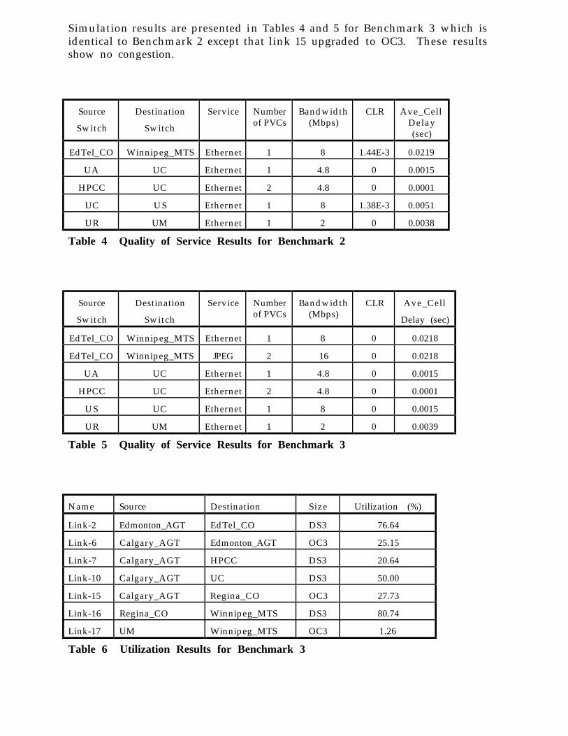
Simulation results are presented in Tables 4 and 5 for Benchmark 3 which isidentical to Benchmark 2 except that link 15 upgraded to OC3. These resultsshow no congestion.

Source

Switch

Destination

Switch

Service Numberof PVCs

Bandwidth(Mbps)

CLR Ave_CellDelay(sec)

EdTel_CO Winnipeg_MTS Ethernet 1 8 1.44E-3 0.0219

UA UC Ethernet 1 4.8 0 0.0015

HPCC UC Ethernet 2 4.8 0 0.0001

UC US Ethernet 1 8 1.38E-3 0.0051

UR UM Ethernet 1 2 0 0.0038

Table 4 Quality of Service Results for Benchmark 2

Source

Switch

Destination

Switch

Service Numberof PVCs

Bandwidth(Mbps)

CLR Ave_Cell

Delay (sec)

EdTel_CO Winnipeg_MTS Ethernet 1 8 0 0.0218

EdTel_CO Winnipeg_MTS JPEG 2 16 0 0.0218

UA UC Ethernet 1 4.8 0 0.0015

HPCC UC Ethernet 2 4.8 0 0.0001

US UC Ethernet 1 8 0 0.0015

UR UM Ethernet 1 2 0 0.0039

Table 5 Quality of Service Results for Benchmark 3

Name Source Destination Size Utilization (%)

Link-2 Edmonton_AGT EdTel_CO DS3 76.64

Link-6 Calgary_AGT Edmonton_AGT OC3 25.15

Link-7 Calgary_AGT HPCC DS3 20.64

Link-10 Calgary_AGT UC DS3 50.00

Link-15 Calgary_AGT Regina_CO OC3 27.73

Link-16 Regina_CO Winnipeg_MTS DS3 80.74

Link-17 UM Winnipeg_MTS OC3 1.26

Table 6 Utilization Results for Benchmark 3

Utilization of Link-15

0.7

0.75

0.8

0.85

0.9

0.95

1

5.1 5

.55.9

6.3

6.7

7.1 7

.57.9

8.3 8

.79.1

9.5 9

.9

10.3

10.7

11.1

11.5

11.9

12.3

12.7

13.1

13.5

13.9

14.3

14.7

15.1

15.5

15.9

16.3

16.7

17.1

17.5

17.9

18.3

18.7

19.1

19.5

19.9

Simulation Time (sec

Link Utilization

Figur e 3 Utilization of Link 15

Average Cell Delay of JPEG1 (Test1)

0.02170.02180.02190.022

0.02210.0222

0.02230.0224

5.1

5.5

5.9 6

.36.7

7.1

7.5

7.9 8

.38.7

9.1

9.5

9.9

10.3

10.7

11.1

11.5

11.9

12.3

12.7

13.1

13.5

13.9

14.3

14.7

15.1

15.5

15.9

16.3

16.7

17.1

17.5

17.9

18.3

18.7

19.1

19.5

19.9

Simulation Time (sec.

Average Cell Delay

(sec.)

Figur e 4 Average Cell Delay for the JPEG1 Load

Standard Deviation of Cell Delay on JPEG1 (Test1

0.00E+00

1.00E-04

2.00E-04

3.00E-04

4.00E-04

5.00E-04

6.00E-04

5.1

5.5

5.9

6.3 6

.77.1

7.5 7

.98.3

8.7

9.1

9.5

9.9

10.3

10.7

11.1

11.5

11.9

12.3

12.7

13.1

13.5

13.9

14.3

14.7

15.1

15.5

15.9

16.3

16.7

17.1

17.5

17.9

18.3

18.7

19.1

19.5

19.9

Simulation Time (sec.)

Standard Deviation

of Cell Delay

Figur e 5 Cell Delay Variation

Current Buffer Occupancy of the Switch Calgary_AGTat the Output Port to Link-15 (Test1)

0

10

20

30

40

50

5.1 5

.55.9

6.3 6

.77.1 7

.57.9 8

.38.7 9

.19.5 9

.9

10.3

10.7

11.1

11.5

11.9

12.3

12.7

13.1

13.5

13.9

14.3

14.7

15.1

15.5

15.9

16.3

16.7

17.1

17.5

17.9

18.3

18.7

19.1

19.5

19.9

Simulation Time (sec.

Current Buffer

Occupancy (cell)

Figur e 6 Buffer Occupancy for the Calgary_AGT Switch

5.2 Telecom New Zealand’s OPERA Experiments

ATM network technology is being evaluated by TeleCom New Zealand, the TuiaSociety and Netway (TeleCom's systems integration company) in a three yearprogram (1996-1998) called OPERA (Organised Programme of Experimentationand Research into ATM). The OPERA network is shown in Figure 7.

Figur e 7 The Telecom New Zealand OPERA Network

There are four main network nodes: two at Massey University, one at WaikatoUniversity, and one at the Crown Research Institute in Dunedin. The TuiaSociety members are the Universities of Auckland, Canterbury, Dunedin,Lincoln, Massey, Victoria and Waikato, plus the Crown Research Institute andthe National Library of NZ.

A preliminary experiment simulating OPERA network operation under abenchmark traffic load was conducted using the ATM-TN Simulator. Thebackbone and edge network connections used in this experiment are shown inFigure 8 below.

The following models and parameter values were used in this experiment:

• Switches are per port with buffers of size 32 packets on each port

• Ethernets were 10 Mb/s links at 30% utilization - bidirectional (SVC)

• One 25 Mb/s MPEG PVC - 1 frame in GOP, 1 for length of recurringsubstructure, 30 frames/sec, smoothing within 1 frame, scaling of 0.8

• Mosaic - 50 conversations at each source/sink, average interarrivaltime between converstions of 5 seconds, destination same probability0.36, 2.5 TCP connections per conversation, mean interarrival timebetween connections in each conversaion of 0.5 sec, and the defaultmessage length specifications

Albany

Waikato

PalmerstonNorth

Dunedin

34Mb, 135km

34Mb, 325km

34Mb, 820km

155Mb, 500m155Mb, 500m155Mb, 500m155Mb, 500m

155Mb, 500m155Mb, 500m155Mb, 500m155Mb, 500m

155Mb, 500m155Mb, 500m155Mb, 500m155Mb, 500m

155Mb, 500m155Mb, 500m155Mb, 500m155Mb, 500m

MPEGEthernetMosaic Source/Sink

Albany

Waikato

PalmerstonNorth

Dunedin

Figur e 8 Network Connections and Links

The simulation results reported for this experiment are intended to illustratehow the simulator can be used. They are not intended to represent a realisticOPERA scenario. Each simulation experiment had a 5 second warmup periodfollowed by 20 seconds of simulated time. Data was collected only during the 20second simulation time, not during warmup. Statistics were collected every 0.1seconds. It took about 16 minutes to run each simulation on a Sparc Server 1000and each run produced around 3.5 Mbytes of data and statistics.

Figures 9 and 10 show the mean and standard deviation of the cell delays for thesingle MPEG traffic stream (from source to sink). Figures 11 and 12 show thesame for cell delays of the Ethernet traffic from Albany to Dunedin (from end toend). Figures 13 and 14 plot the average and standard deviation of the cell delaysof all traffic that crosses the Albany-Waikato link.

Figures 15 and 16 show the buffer occupancy at the Palmerston North outputbuffer of the Waikato switch (the first is scaled to the buffer size (32) and thesecond is scaled to the maximum occupancy (2)). Figures 17 and 18 show theutilisation of the Albany-Waikato link (the second Figure is scaled to make thedifferences stand out more). Figure 19 plots the number of cells dropped overthe Albany-Waikato link. This illustrates that even though the link neverreaches full utilisation some cells are still lost. In this case all the cells droppedwere from the Mosaic traffic. Finally, the cell delay for each traffic source andsink stream is presented in Table 7.

Average Cell Delay for MPEG

0.001757

0.0017575

0.001758

0.0017585

0.001759

0.0017595

0.00176

0.0017605

0.001761

55.4

5.8

6.2

6.6 7

7.4

7.8

8.2

8.6 9

9.4

9.8

10.2

10.6 1

1

11.4

11.8

12.2

12.6 1

3

13.4

13.8

14.2

14.6

15

15.4

15.8

16.2

16.6 1

7

17.4

17.8

18.2

18.6 1

9

19.4

19.8

Simulation Tim

Average Cell Delay

(sec.)

Figur e 9 Average MPEG Cell Delay

Standard Deviation of Cell Delay for MPEG

0.00E+00

1.00E-06

2.00E-06

3.00E-06

4.00E-06

5.00E-06

6.00E-06

7.00E-06

55.4

5.8

6.2

6.6 7

7.4

7.8

8.2

8.6 9

9.4

9.8

10.2

10.6 1

1

11.4

11.8

12.2

12.6 1

3

13.4

13.8

14.2

14.6 1

5

15.4

15.8

16.2

16.6 1

7

17.4

17.8

18.2

18.6 1

9

19.4

19.8

Simulation Time (sec

Standard Deviation

of Cell Delay (sec.)

Figure 10 Standard Deviation of MPEG Cell Delay

Average Cell Delay of Ethernet From Albany to Dunedi

0.004811

0.004812

0.004813

0.004814

0.004815

0.004816

0.004817

0.004818

0.004819

55.4

5.8

6.2

6.6 7

7.4

7.8

8.2

8.6 9

9.4

9.8

10.2

10.6 1

1

11.4

11.8

12.2

12.6 1

3

13.4

13.8

14.2

14.6 1

5

15.4

15.8

16.2

16.6 1

7

17.4

17.8

18.2

18.6 1

9

19.4

19.8

Simulation Tim

Average Cell Delay

(sec.)

Figure 11 Average Ethernet Cell Delay (Albany to Dunedin)

Standard Deviation of Cell Delay for Ethernet from Albany to Dunedi

0.00E+00

2.00E-06

4.00E-06

6.00E-06

8.00E-06

1.00E-05

1.20E-05

1.40E-05

55.4

5.8

6.2

6.6 7

7.4

7.8

8.2

8.6 9

9.4

9.8

10.2

10.6 1

1

11.4

11.8

12.2

12.6 1

3

13.4

13.8

14.2

14.6 1

5

15.4

15.8

16.2

16.6 1

7

17.4

17.8

18.2

18.6 1

9

19.4

19.8

Simulation Tim

Standard Deviation

of Cell Delay (sec.)

Figure 12 Standard Deviation of Ethernet Cell Delay (Albany to Dunedin)

Average Cell Delay Over Albany-Waikato Link

0

0.0001

0.0002

0.0003

0.0004

0.0005

0.0006

0.0007

5.1

5.5

5.9

6.3

6.7

7.1

7.5 7

.98.3

8.7

9.1

9.5

9.9

10.3

10.7

11.1

11.5

11.9

12.3

12.7

13.1

13.5

13.9

14.3

14.7

15.1

15.5

15.9

16.3

16.7

17.1

17.5

17.9

18.3

18.7

19.1

19.5

19.9

Simulation Tim

Average Cell Delay

(sec.)

Figure 13 Average Cell Delay (Alban y - Waikato)

Standard Deviation of Cell Delay Over Albany-Waikato Link

0

0.0001

0.0002

0.0003

0.0004

0.0005

0.0006

5.1

5.5

5.9

6.3

6.7

7.1

7.5 7

.98.3

8.7

9.1

9.5

9.9

10.3

10.7

11.1

11.5

11.9

12.3

12.7

13.1

13.5

13.9

14.3

14.7

15.1

15.5

15.9

16.3

16.7

17.1

17.5

17.9

18.3

18.7

19.1

19.5

19.9

Simulation Tim

Standard Deviation

of Cell Delay (sec.)

Figure 14 Standard Deviation of Cell Delay (Alban y - Waikato)

Current Buffer Occupancy of the Waikato Switch at Palmerston North Output P

0

4

8

12

16

20

24

28

32

55.4 5

.86.2 6

.6 77.4

7.8 8

.28.6 9

9.4 9

.8

10.2

10.6 1

1

11.4

11.8

12.2

12.6 1

3

13.4

13.8

14.2

14.6 1

5

15.4

15.8

16.2

16.6 1

7

17.4

17.8

18.2

18.6 1

9

19.4

19.8

Simulation Tim

Current Buffer

Occupancy (cell)

Figure 15 Buffer Occupancy at Palmerston North Port of Waikato Switch

Current Buffer Occupancy of the Waikato Switch at Palmerston North Output P

0

0.5

1

1.5

2

55.4

5.8 6

.26.6 7

7.4 7

.88.2 8

.6 99.4 9

.8

10.2

10.6 1

1

11.4

11.8

12.2

12.6 1

3

13.4

13.8

14.2

14.6 1

5

15.4

15.8

16.2

16.6 1

7

17.4

17.8

18.2

18.6 1

9

19.4

19.8

Simulation Tim

Current Buffer

Occupancy (cell)

Figure 16 Buffer Occupancy at Palmerston North Port of Waikato Switch

Utilisation of Albany-Waikato Link

0

0.1

0.2

0.3

0.4

0.5

0.6

0.7

5.1

5.5

5.9 6

.36.7

7.1 7

.57.9

8.3

8.7 9

.19.5

9.9

10.3

10.7

11.1

11.5

11.9

12.3

12.7

13.1

13.5

13.9

14.3

14.7

15.1

15.5

15.9

16.3

16.7

17.1

17.5

17.9

18.3

18.7

19.1

19.5

19.9

Simulation Tim

Link Utilisation

Figure 17 Alban y - Waikato Link Utilization

Utilisation of Albany-Waikato Link

0.4

0.45

0.5

0.55

0.6

0.65

5.1 5

.55.9

6.3

6.7 7

.17.5

7.9 8

.38.7 9

.19.5

9.9

10.3

10.7

11.1

11.5

11.9

12.3

12.7

13.1

13.5

13.9

14.3

14.7

15.1

15.5

15.9

16.3

16.7

17.1

17.5

17.9

18.3

18.7

19.1

19.5

19.9

Simulation Tim

Link Utilisation

Figure 18 Alban y - Waikato Link Utilization

Cells Dropped on Albany-Waikato Link

0

50

100

150

200

250

300

350

5.1

5.5

5.9 6

.36.7

7.1 7

.57.9

8.3 8

.79.1

9.5 9

.9

10.3

10.7

11.1

11.5

11.9

12.3

12.7

13.1

13.5

13.9

14.3

14.7

15.1

15.5

15.9

16.3

16.7

17.1

17.5

17.9

18.3

18.7

19.1

19.5

19.9

Simulation Tim

Cells Dropped

Figure 19 Cells Dropped on the Alban y - Waikato Link

Source Destination Service Expected

Delay

Average

Delay

Max

Delay

Standard

Deviation

Albany Waikato Ethernet 0.000536247 0.000541674 0.000586182 7.10321e-06

Waikato Albany Ethernet 0.000536247 0.00053737 0.000551918 2.84322e-06

Albany Palmerston

North

Ethernet 0.00175522 0.00176465 0.00184929 1.0571e-05

Palmerston

North

Albany Ethernet 0.00175522 0.00175772 0.00179254 4.60184e-06

Albany Dunedin Ethernet 0.00480569 0.00481581 0.00489959 1.09092e-05

Dunedin Albany Ethernet 0.00480569 0.0048092 0.00486004 5.68489e-06

Waikato Palmerston

North

Ethernet 0.00123925 0.00124534 0.00129872 7.36815e-06

Palmerston

North

Waikato Ethernet 0.00123925 0.00124117 0.00127326 3.92735e-06

Waikato Dunedin Ethernet 0.00428972 0.00429651 0.00434753 7.73641e-06

Dunedin Waikato Ethernet 0.00428972 0.0042924 0.00433996 4.99129e-06

Palmerston

North

Dunedin Ethernet 0.00307075 0.00307184 0.00308322 2.80559e-06

Dunedin Palmerston

North

Ethernet 0.00307075 0.00307186 0.00309524 2.98747e-06

Albany Palmerston

North

MPEG 0.00175522 0.00175981 0.00178253 5.67449e-06

Table 7 Cell Delay for Each Traffic Source and Sink Stream

6. Performance of the ATM-TN Simulator

Preliminary performance results are presented in Figure 20 below for the Wnetbenchmark experiments of section 5.2 using optimistic synchronization andWarpKit. These represent results for a simulation of Wnet executed on from 1 to12 Silicon Graphics R8000 CPUs for an SGI PowerChallenge multiprocessorplatform. The dotted line represents perfect speedup, ie., a simulation runs 4times faster on 4 processors (CPUs).

The “relative” speedup is defined as the time it takes to run the simulation on 1processor divided by the time it takes on “n” processors using identical software.The latter refers to the parallel system consisting of the Wnet model and scenarioon the ATM-TN on SimKit and on WarpKit. The “absolute” speedup is definedin the same way except the sequential execution time for the optimizedsequential system (OSS) is used rather than the WarpKit time on 1 processor.

This shows an effective (absolute) speedup of 4.4 on 12 processors. This resultsuggests that parallel execution on a multiprocessor platform may significantlyreduce the required time to execute a simulation experiment. However, therewas considerable additional complexity in the Wnet model required to enableparallel execution. It is also not clear that this level of speedup is possible with arange of network models and traffic load scenarios.

Speedup

1 2 4 8 12

8

4

2

7.2

4.4

3.4

1.9

3.2

5.6

absolute

relative

•

•

•

•

•

•

SGI Powerchallenge R8000 Processors

•

•

1.1

1.8

••0.6

Figure 20 Preliminary Simulator Performance for the Wnet Scenario

7. Conclusions

The preliminary experiments conducted for the Wnet and OPERA scenariosstrongly suggest that the dynamic behavior of an ATM network can be adequatelycaptured using simulation. Dynamic cell loss, cell delay and cell delay variationcan all be produced using the ATM-TN simulator. Although failures were notintroduced in these experiments, it would be relatively easy to introduce a broadrange of dynamic and static failure types. Further experiments will be needed,however, to quantify the accuracy of simulation results.

The speed of execution of the ATM-TN simulator is marginally adequate forscenarios of ten to one hundred ATM switches and ten to one hundred trafficsource /sink streams. The Wnet scenario running sequentially on 1 SGI R8000CPU takes about 70 CPU execution seconds per simulated second withoutcompiler optimization. Thus it takes about 70 minutes to simulate 1 minute or11.5 hours to simulate 10 minutes of Wnet operation.

With the compiler optimization flag “on” this might be reduced to 50 CPUseconds per simulated second or about 8.5 hours for 10 minutes. On twelveprocessors this would be reduced by the factor of 4.4 shown in Figure 20, givingless than 2 hours to simulate 10 minutes of Wnet operation.

Further speedup via parallel execution may also be possible with a newconservative synchronization mechanism that is described in the paper ofAppendix B. Ultimately this may require less added model source codecomplexity than needed for the optimistic methods of WarpKit.

There are also many situations where a cell level simulation will not be needed.Siemens has made modifications to the ATM-TN to ignore all data cells, ie., onlySVC set up and tear down control cells are simulated with one scheduled delayfor the data cells across each SVC. Their preliminary experience with this call-level version of the ATM-TN shows performance of about 60 calls per CPUsecond on a Sparc 10 for a path of two endnodes and three switches. This meansabout 12 seconds on a Sparc 10 to simulate a busy hour (3,600 seconds) for an E1line with a capacity of 32 telephone connections (PCR=150).

In conclusion, the simulation of ATM traffic and networks is both feasible andpractical. It is expected that adequate accuracy can be achieved to predict dynamicnetwork behavior under varying traffic loads and failures. Further validationexperiments will be needed to quantify the accuracy of such simulations.

Long simulation execution times are required to perform simulations of realisticATM network and traffic scenarios. Currently these can be as high as 12 hours toexecute a 10 minute network simulation. However, techniques are beingexplored that can substantially reduce these execution times. Preliminary resultsalready show that this 12 hour execution time can be reduced to less than 2 hoursfor a 10 minute cell-level simulation of a 12 switch, 8 traffic stream scenario.

BibliographyAbrams, M. 1988. "The Object Library for Parallel Simulation”, Proceedings of the1988 Winter Simulation Conference, San Diego, California, 210--219, December.

Abrams, M. 1989. " A Common Interface for Chandy-Misra, Time-Warp, andSequential Simulators", Proceedings of the 1989 Winter Simulation Conference,Washington, D.C., December.

Abrams, M. and Lomow, G. 1990. "Issues in Languages for Parallel Simulation",Proceedings of the 1990 SCS Multiconference on Distributed Simulation, 22(2)",San Diego, California, 227--228, January.

ACM. 1995. Special Edition on “Issues and Challenges in ATM Networks”,Communications of the ACM.

Arlitt, M., Chen, Y., Gurski, R. and Williamson, C.L. 1995a. “Traffic Modeling inthe ATM-TN TeleSim Project: Design, Implementation, and PerformanceEvaluation”, Proceedings of the 1995 Summer Computer Simulation Conference,Ottawa, Ontario, July.

Arlitt, M. and Williamson, C.L. 1995b. “A Synthetic Workload Model for InternetMosaic Traffic”, Proceedings of the 1995 Summer Computer SimulationConference, Ottawa, Ontario, July.

ATM Forum. 1993. “ATM User-Network Interface Specification”, Version 3.0,Prentice Hall, New Jersey.

Bagrodia, R. and Liao, W.T. 1990. "Maisie: A Language and OptimizingEnvironment for Distributed Simulation", Proceedings of the 1990 SCSMulticonference on Distributed Simulation, San Diego, California, 22(2), 205--210,January.

Baezner, D., Lomow, G.A. and Unger, B.W. 1994. “A Parallel SimulationEnvironment Based on Time Warp”, International Journal in ComputerSimulation, 4(2), 183-207.

Baezner, D. and Lomow, G. and Unger, B. 1990. “Sim++: The Transition toDistributed Simulation", Proceedings of the 1990 SCS Multiconference onDistributed Simulation, San Diego, California, 22(2), 211--218, January.

Chandy, K. M. and Misra, J. 1979. “Distributed Simulation: A Case Study inDesign and Verification of Distributed Programs", IEEE Transactions on SoftwareEngineering", SE-5, 440--452, September.

Chandy, K. M. and Misra, J. 1981. "Asynchronous Distributed Simulation via aSequence of Parallel Computations", Communications of the ACM, 24(11), 198--206, April.

Chen, Y., Deng, Z. and Williamson, C.L. 1995. “A Model for Self-Similar EthernetLAN Traffic : Design, Implementation and Performance Implications”,Proceedings of the 1995 Summer Computer Simulation Conference, Ottawa,Ontario, July.

Cleary, J. and Gomes, F. and Unger, B. and Zhonge, X. and Thudt, R. 1994. "Costof State Saving and Rollback", Proceedings of the 8th Workshop on Parallel andDistributed Simulation (PADS94), Edinburgh, Scotland, 24(1), 94--101, July.

Ferscha, A. and Tripathi, S. K. 1994. "Parallel and Distributed Simulation ofDiscrete Event Systems", Technical Report CS-TR-3336, Department of ComputerScience, University of Maryland, College Park, MD, August.

Fujimoto, R. 1993. "Parallel and Distributed Discrete Event Simulation:Algorithms and Applications", Proceedings of the 1993 Winter SimulationConference Proceedings, Los Angeles, 106--114, December.

Fujimoto, R. and Nicol, D. 1992. "State of the art in Parallel Simulation",Proceedings of the 1992 Winter Simulation Conference", Arlington, Virginia, 25,246-254, December.

Fujimoto, R. M. 1990a. "Parallel Discrete Event Simulation", Communications ofthe ACM, 33(10), 33-53, October.

Fujimoto, R., 1990b. “Time Warp on a Shared Memory Multiprocessor",Transactions of the Society of Computer Simulation, 6(3), 211-239, July.

Fujimoto, R.M. 1990c. “Parallel Discrete Event Simulation”, Communications ofthe ACM, 33(10), 30-53.

Gburzynski, P., Ono-Tesfaye, T. and Ramaswamy, S. 1995. “Modeling ATMNetworks in a Parallel Simulation Environment: A Case Study”, Proceedings ofthe 1995 Summer Computer Simulation Conference, Ottawa, Ontario, July.

Ghosh, K. and Fujimoto, R. 1991. "Parallel Discrete Event Simulation UsingSpace-Time Memory", Proceedings of the International Conference on ParallelProcessing, 3, 201-208, August.

Gill, D. H. and Maginnis, F. X. and Rainier, S. R. and Reagan, T. P. 1989. "AnInterface for Programming Parallel Simulations", Proceedings of the SCSMulticonference on Distributed Simulation (eds Unger, B. and Fujimoto, R.),Tampa, Florida , 21(2), 151-154, March.

Gomes, F. (1996) “Optimizing Incremental State Saving and Restoration”, Ph.D.thesis, in progress, Department of Computer Science, University of Calgary.

Gomes, F., Cleary, J., Covington, A., Franks., S., Unger, B., and Xiao, Z. 1995.“SimKit: A High Performance Logical Process Simulation Class Library in C++”,Proceedings of the 1995 Winter Simulation Conference, Washington D.C.,December.

Gurski, R., Williamson, C., Arlitt, M., Covington, A., Gburzynski, P., Gomes, F.,Ono-Tesfaye, T., Ramaswamy, S., Unger, B.W. & Xiao, Z. 1995. “ATM-TN UserManual”, WurcNet Technical Report, July, 12 pages.

Hassam, R. 1991. “SIMA: A Parallel Simulation Environment", Technical ReportTRITA--TCS--91007, Dept. of Telecomm. and Computer Science, The RoyalInstitute of Technology, S--10044, Stockholm, Sweden.

Jefferson, D.R. 1985. "Virtual Time", ACM Transactions on ProgrammingLanguages and Systems, 7(3), 404-425, July.

Marti, J. 1988. "RISE: The RAND Integrated Simulation Environment",Proceedings of the 1988 SCS Multiconference on Distributed Simulation (edsUnger, B. & Jefferson, D.), San Diego, Calif., 19(3), 68--72, February.

Mehl, H. and Hammes, S. 1993. "Shared Variables in Distributed Simulation",Proceedings of the 7th Workshop on Parallel & Distributed Simulation(PADS93), San Diego, California, 23(1), 68-75, July.

Melamed, B. and Hill, J. 1995. “A Survey of TES Modeling Applications”,Simulation 64 (6), 353 - 370, June.

Nikolaidis, I. and Onvural, R.O. 1992. “A Bibliography of Performance Issues inATM Networks” Computer Communication Review, ACM Sigcomm, 22(5), 8-23.

Page, E. H. and Nance, R. E. 1994. "Parallel Discrete Event Simulation: AModeling Methodological Perspective", Proceedings of the 8th Workshop onParallel and Distributed Simulation (PADS94), Edinburgh, Scotland, 24(1), July.

Pearson, M., Cleary, J., Unger, B. and Williamson, C. 1996 “Current Techniquesfor Measuring and Modeling ATM Traffic” Technical Report, Computer ScienceDepartment, Waikato University, 36 pages.

Perloff, M. and Reiss, K. 1995. “Improvements to TCP Performance in High-Speed ATM Networks” Communications of the ACM, 90-109, February.

Preiss, B. R. 1989. "The Yaddes Distributed Discrete Event SimulationSpecification Language", Proceedings of the SCS Multiconference on DistributedSimulation, Tampa, Florida, 21(2), 139--144, March.

Rajaei, H. and Ayani, R. 1992. “Language Support for Parallel Simulation",Proceedings of the 6th Workshop on Parallel and Distributed Simulation(PADS92), New Port Beach, California, 24(3), 191--192, January.

Reynolds, Jr. P. 1988. " A spectrum of options for parallel simulation",Proceedings of the 1988 Winter Simulation Conference, San Diego, California,325--332, December.

Rich, D. O. and Michelsen, R. E. 1991. "An assessment of the ModSim / TWOSParallel Simulation Environment", Proceedings of the 1991 Winter SimulationConference, 509--517, December.

Unger, B.W., Goetz D.J. and Maryka, S.W. 1994a. "The Simulation of SS7Common Channel Signaling", IEEE Communications, 32(3), 52-62.

Unger, B.W. and Xiao, Z. 1994b. “The Fast Parallel Simulation ofTelecommunication Networks”, Proceedings of the 1994 Conference on NewDirections in Simulation for Manufacturing and Communications, OperationsResearch Society of Japan, 9-16, August.

Unger, B.W., Arlitt, M., Gburzynski, P., Gomes, F., Gurski, R., Ono-Tesfaye, T.,Ramaswamy, S., Williamson, C. and Xiao, Z. 1994c. “ATM-TN System Design”,WurcNet Technical Report, September, 142 pages.

Unger, B.W. and Cleary, J.G. 1993. “Practical Parallel Discrete Event Simulation”ORSA Journal on Computing,, 5(3), 242-244.

Unger, B.W., Cleary, J. G., Dewar, A. and Xiao, Z. 1990. " A Multi-LingualOptimistic Distributed Simulator", Transactions of the Society for ComputerSimulation, 7 (2), 121-152, June.

Vickers, B.J., Kim, J.B., Suda, T. and Hong, D.P. 1993. “Congestion Control andResource Management in Diverse ATM Environments”, IEICE Transactions onCommunications, November.

Waldorf, J. and Bagrodia, R. 1994. "MOOSE: A Concurrent Object-OrientedLanguage for Simulation", International Journal in Computer Simulation, 4(2),235--257.

West, J. and Mullarney, A. 1988. "ModSim: A Language for DistributedSimulation", Proceedings of the 1988 SCS Multiconference on DistributedSimulation, (eds Unger B. and Fujimoto, R.), San Diego, California, 19(3), 155--159 February.