Adaptive localization and adaptive inflation methods with the LETKF

JOURNAL OF COMPUTATIONAL AND APPLIED MATHEMATICS
ELSEVIER Journal of Computational and Applied Mathematics 81 (1997) 115-134
High order adaptive methods of Nystr6m-Cowell type
J .M. F r a n c o * , J .F . P a l a c i a n
Departamento de Matemdtica Aplicada, Escuela Tbcnica Superior de Ingenieros lndustriales, Universidad de Zaragoza, 50015-Zaragoza, Spain
Received 28 June 1995
Abstract
A class of unconditionally stable multistep methods is discussed for solving initial-value problems of second-order differential equations which have periodic or quasiperiodic solutions. This situation frequently occurs in celestial mechanics, in nonlinear oscillations and various other situations. The methods depend upon a parameter co > 0, and integrate exactly trigonometric functions along with algebraic polynomials. In this paper we show a procedure for the construction of adaptive Nystr/Sm-Cowell formulas of arbitrarily high order of accuracy, and reduce to the classical NystriSm-Cowell methods for co = 0. Our methods compare advantageously with other methods.
Keywords: Second-order initial-value problems; Adaptive Nystr6m-Cowell methods; Orbital unstability
AMS classification: 65L05; 65L20
1. Introduction
In this paper we present new methods , which we call adapt ive Nystr /Sm-Cowell methods , for the numerical in tegra t ion of second-order initial-value problems of the form
d 2 y + c o 2 y = f ( t , y ) , O < t < . T , c o > 0 , y e R " , dt 2
(1.1) y(0) = Yo, y'(0) = y~,
where the main frequency co m a y be k n o w n or accurately es t imated and the per turbing fo rce f ( t , y) is assumed to be small relative to the force co2y, i.e. f ( t , y) = eg(t, y), e being a small pa ramete r (e < 1). These me thods are designed in such a way that , for the unper tu rbed p r o b l e m f ( t , y) = 0, the error of the free oscillations in the numerical solut ion is null. In other words, the me t h o d s presented
* Corresponding author. E-mail: [email protected]
0377-0427/97/$17.00 © 1997 Elsevier Science B.V. All rights reserved PII S 0 3 7 7 - 0 4 2 7 ( 9 7 ) 0 0 0 3 0 - 7
116 J.M. Franco, J.F. Palacian/Journal of Computational and Applied Mathematics 81 (1997) 115-134
integrate exactly the unperturbed problem. Methods having this property are suitable for long interval integration of perturbed systems of type (1.1), because the integration step size may be chosen much larger than the step size needed for classical multistep methods. Besides, the numerical deficiency known as orbital unstability (see [11]) is avoided.
In several previous papers, [4, 9], we have introduced and studied a class of adaptive St6rmer-Cowell methods. The adaptive Nystr6m-Cowell methods are different from the adaptive St6rmer-Cowell methods by the way they choose the coefficients at each step of the integration. The new selection is meant to improve the efficiency of the adaptive St6rmer-Cowell methods and the other classical multistep methods. That they do so, we shall show in Section 4.
In order to integrate the initial-value problem (1.1), it is desirable to use methods that do not require introducing the derivatives y' since they are not explicitly contained in the perturbation force. Assuming the main frequency of oscillation is a priori known (exactly or to a good approximation), a kind of adaptive St6rmer-Cowell formula for the numerical integration of Eq. (1.1) has the form [9].
k k
ctj(v)y,+j = h 2 ~ flj(v)f(t,+j, y,+j), v = coh, (1.2) j = 0 j = 0
where the coefficients ccj(v) and flj(v) are assumed to be continuous functions for each v e [0, A], for an A > 0 given. The development of the integration procedure (1.2) follows the idea given in Correas (1977, 1978) and it is characterized by the linear truncation error operators Lh, defined as follows:
k Lh[y(t)] = ~ [o~j(v)y(t + jh) - h2flj(v){y"(t + jh) + c02y(t +jh)}]. (1.3)
i=0
Furthermore, Correas imposes that the kernel of Lh contain the linear spaces Hp(co) generated by the modified Stumpff functions qSi(t, co), i = 0, 1, . . . , p, where
q~°(t' co) = {C°Slcot ifif co ~0 ,co =0,
¢i+l(t, co) = fi ¢i(t, o)dt, i>~O.
The linear space lip(co) generated by the functions ~,bi(t, co) may be expressed in the form
~Span{1, t, t z , . . . , t p- 2, cos cot, sin cot} if co ~ 0, Hv(~°) = ~Span{1, t, t 2, , tv-2, t v - l , t p} if co = 0.
Consequently, if co = 0, the difference equations (1.2) reduces to the classical multistep methods with constant coefficients.
The connection between spaces Hv(co ), the linear operators Lh and the order of consistency of the methods are as follows [9].
J.M. Franco, J.F. Palacian/Journal of Computational and Applied Mathematics 81 (1997) 115-134 117
Order conditions: The linear operator Lh associated with the adaptive method (1.2) annihilates the space Pip+ l(e)) if and only if the following conditions are verified:
k Do = ~ ~j(v)dpo(j, v) = O,
j=O k
D1 = Z O~J(V)~Pl(J' v) ----0, (1 .4 ) j = o
k
Oi = 2 [{o~j(1)) - - v2flj(v)}~gi(j, v) -- flj(v)dpi_e(j, v ) ] = 0, i =2, 3, . . . , p + 1. j=O
Besides, these conditions are sufficient at order p for all co real. The necessary and sufficient conditions are
Do = 0(hp+2), D, =0(h p+') . . . . ,Dp+ 1 =0(h). (1.5)
Under the hypothesis of consistency of order one and the following roots condition If ~(v) is a root of p(~, v), there exists a positive constant C such that [~(v)[ ~< exp(Cv). Besides, if ~(v) is a root of p(~, v) with multiplicity greater than two, then ]~(v)l < 1 for all v e [0, A],
the method (1.2) is convergent (see [4, 9]).
Definition. We call the method (1.2) an adaptive Nystr6m-Cowell (adaptive-NC) method if
~k(V) = 1, C~k-2(V) = --2 4)0(2, V), ~k-4(V) = 1,
~j(V)=0, j ~ k , k - 2 , k - 4 ,
To distinguish them from the methods characterized by the conditions
C~g(V) =1, ~ k - l ( V ) = --2 qS0(1, v), C~k-2(V) =1,
ej(V) =0, j ¢ k , k - l , k - 2 ,
we shall call the latter the adaptive St6rmer-Cowell (adaptive-SC) methods. In Section 2, we construct an accurate and efficient procedure for the integration of dynamical
systems of type (1.1), These algorithms are built for arbitrarily high order of accuracy; they are very easy to implement in a digital computer. Besides, we prove that the local truncation error constants of the adaptive-NC methods are smaller than that corresponding to the adaptive-SC methods. This feature was already known (see [5]) for the classical methods of constant coefficients (v = 0). In Section 3, the stability of the adaptive methods is discussed using the standard linear test model. In Section 4, we compare numerically these methods to adaptive St~Srmer-Cowell methods [4, 9] and other classical ones. We conclude with a few results from the numerical experiments realized.
2. Derivation of the adaptive Nystr6m-Cowell methods
One may think of constructing adaptive methods by solving the linear system given by conditions (1.4). The process, however, is unsuitable in practice for methods of a high order. As an
118 J.M. Franeo, J.F. P alacian /Journal of Computational and Applied Mathematics 81 (1997) 115-134
example of the complexity one would encounter, see the paper of Neta and Ford [-8]. One overcomes the difficulty by means of recurrent algorithms for a class of adaptive methods, namely the Nystr6m-Cowell methods.
To this effect, the general solution of problem (1.1) can be written as
~ ' f ( s )¢ l ( t y(t) = C14)o(t, co) + C2cbl(t, co) + - s, co) ds, (2.1)
where C1 and C2 are arbitrary constants, co is the main frequency of problem (1.1). By an abuse of notation, we write f(s) to designate f(s,y(s)). Substituting t.+i, t, and t , - i for t in (2.1) and eliminating C~ and C2 from the resulting equations, we obtain
f t n + i
y(t,+i) --2q$0(i, v)y(t,) + y(t,-i) = [f(s) + f ( Z t , -- s)] q$1(t,+i - s, e)) ds, • ) tn
with v = coh. This equation is obtained for the case i = 1 in [4], and it is used for the construction of adaptive-SC methods. In this section, we study the case i - - 2 to build high-order adaptive-NC methods. Substituting the perturbing functionf(t , y) by the Newton backward difference interpola- tion polynomial in a mesh of equally spaced points tj = to + jh, (0 <<, j <~ k), we obtain the following adaptive multistep method
k Y.+2 -24)0(2, v)y. + Y,-2 = h 2 ~ ~,,(v) 17sf.+,, r =1, 2, (2.2)
j = 0
where r = 1 in the explicit case, and r = 2 in the implicit one. In (2.2) I7% is the j th backward difference and J~ =f(tk , Yk). The coefficient o-j,,(v) are given by the quadratures: for the explicit case
o-i, (v) ( - 1 ) J f : x [ ( j , = - ~ j + \ ~ j 2 j _ ] c ~ ( 1 - ~ , v ) d ~ , (2.3a) I ( .+ l l for the implicit case
O'J, 2 (10 ( - - 1 ) J f ° 2 I ( j = - "c) + C ; 4 ) ] ~ b ~ ( - ~, v) d~. (2.3b)
These coefficients can be computed in a simple and recurrent form, thereby producing analytic functions G,(t, v) (generating functions); in this manner, the coefficients o-j,,(v) are precisely the coefficients of G,(t, v) expanded as a Taylor series at t = 0 [5].
Consider the generating functions of the form
G,(t ,v)= ~ ~j,,(v)t j, r = l , 2. j = 0
Substituting the values (2.3) of the coefficients o-s,,(v ) and integrating by parts, we obtain the following generating functions:
2(1 - q$o(2, v))(1 - 02 + 4t 2 - 4t 3 - t 4 G,(t, v) = [(r - 1) + (2 - r)(1 - t)] [(log(1 - t)) 2 + v2] ' r = 1, 2. (2.4)
J.M. Franco, J.F. Palacian/Journal of Computational and Applied Mathematics 81 (1997) 115-134 119
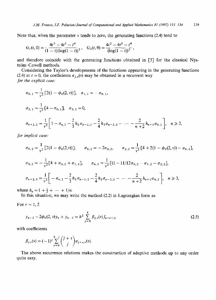
Note that , when the pa ramete r v tends to zero, the generat ing funct ions (2.4) tend to
4t 2 - - 4 t 3 - - t 4 Gl(t,O) = (1 -- t)(log(1 -- t)) 2 ' G2(t,O) =
4t 2 -- 4 t 3 - - t 4
(log(1 - t)) 2 '
and therefore coincide with the generat ing funct ions ob ta ined in [-5] for the classical Nys- t r6m-Cowel l methods .
Consider ing the Taylor ' s developments of the funct ions appear ing in the generat ing funct ions (2.4) at t = 0, the coefficients 0.j, r(v) m a y be obta ined in a recurrent way for the explicit case:
1 0.0, 1 = ~-~ [2(1 - q5o(2, v))], a l , 1 = - - 0.0, 1,
1 0.2, 1----~-~ [ 4 - 0"0.1], 0 - 3 , 1 = 0 ,
1 E o . + 2 , 1 = ~ 1 - o . , 2 2
1 - ~ h 2 ° ' n - l . l - ~ h 3 0 . n - 2 , 2 q
h,+10.o,1/ , n i > 2 , x - • n + 2 A
for implicit case,"
1 0.o, 2 = ~ [2(1 - ~bo(2,v))], 0"1, 2 = --20.0,2,
1 0.2,2 = ~ [4 +2 (1 - q5o(2, v)) - Oo,2],
1 0-3, 2 = - - ~ - ~ [ 4 + 0"0,2 + 0"1,2],
1 0.4,2 =~-~ [(1 - 11/120.o,2 - 0.1,2 - 0.2,2],
1 [- 2 2 2 0"n+2'2 = "~ L - - 0.n, 2 - - ~ h2 ° 'n- 1,2 - - ~ h3 0"n-2,2 r / + ~ hn+ 160,2
1 where h. = 1 + ~ + ... + 1In. In this si tuation, we m a y write the m e t h o d (2.2) in Lagrang ian form as
, n~>3,
F o r r - 1, 2
k Y.+2 -2~bo(2, v)y. + Y.-2 = h 2 ~ flj, r(v)f.+r-j, (2.5)
j=O
with coefficients
k j ( ) /b,r(vt = ( - 1/j J + s
s=o J
The above recurrence relat ions makes the cons t ruc t ion of adapt ive me thods up to any order quite easy.
120 J.M. Franco, J.F. Palacian/Journal o f Computational and Applied Mathematics 81 (1997) 115-134
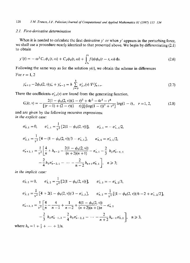
2.1. First-derivative determination
W h e n it is needed to ca lcu la te the first de r iva t ive y ' or w h e n y ' appea r s in the p e r t u r b i n g force, we shall use a p r o c e d u r e nea r ly ident ica l to t h a t p re sen ted above . W e begin by d i f fe ren t ia t ing (2.1) to o b t a i n
ftl f ( s ) y'(t) = - cozcld~l(t , co) + C2~bo(t, co) + ~bo(t - s, co)ds. (2.6)
F o l l o w i n g the s ame w a y as for the so lu t ion y(t), we o b t a i n the scheme in differences
F o r r = 1, 2
k Y~+2 -2q5o(2, v)y~ + Y ' - 2 = h ~ a~,r(v) Wf ,+r . (2.7)
j=0
There the coeff icients aj, r(v) are f o u n d f r o m the gene ra t i ng func t ion ,
2(1 - q5o(2, v))(1 - 02 + 4t 2 - 4 t 3 - t 4 G'(t, v) = [(r - 1) + (2 - r)(1 - t)] [( log(1 - 0) 2 + v 2] log(a - t ) , r = 1, 2, (2.8)
a n d are given by the fo l lowing recurs ive express ions: in the explicit case:
1 a ,l = 0 , °1'1 = 7 [2(1 -- ~bo(2, v))], 0-~,1 = - a~, 1/2,
1 0-~,1 = ~ [4 - (1 - q~o(2, v))/3 - 0-~, 1],
1E4 0-;+2,1 = O +hn-2 - -
2(1 -- 4,o(2, v))
(n + 2 ) ( n + 1 )
2 4 h3° 'n -2 ' l - "
in the implicit case."
! 0-0.2 ~ O~
' ' / 2 0-4,1 ~ 0"3,1 ,
2 -- 0- n, 1 - - -~ h z 0- ; -1,1
2 h , + l o ' ~ , l l , n~>3 ;
n + 2 A
0-i, z = ~ [2(1 - ~bo(2, v))], o~, 2 = - 0-i, 2/3,
1 0-;,2 = ~-g [4 + 2(1 -- q~o(2, v))/3 - o i , 2],
1 [ ! 4 1 4(1 - o(2, v)) 0-, 0";+2'2 = - ~ _ n - ~ l +-nZ--2--2 + (n + 2)(n + l )n - n, 2
2 h20- ,~-1 ,2- ' , 3 ~ h30-;-2,2 n + 2 h,+10-o,2
where h, = 1 + 1 + ... + 1/n.
1 0-#,2 = ~-g [(1 -- q5o(2 , v))/6 - -2 + 0-~, 2/2] ,
n~>3 ,
J.M. Franco, J.F. Palacian/Journal of Computational and Applied Mathematics 81 (1997) 115-134 121
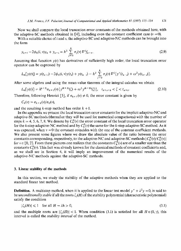
Now we shall compare the local truncation error constants of the methods obtained here, with the adaptive-SC methods obtained in [4], including even the constant coefficient case (v =0).
With a suitable choice of i and s, the adaptive-SC and adaptive-NC methods can be brought into the form
k
y,+, -2q5o(i, v)y, + y._, = h 2 ~ aj(v) VJf,+~. (2.9) j = 0
Assuming that function y(t) has derivatives of sufficiently high order, the local truncation error operator can be expressed by
k
Lh[y(t)] = y(t,+i) --2q~o(i, v)y(t,) + y(t , - i ) -- h 2 ~ aj(v) VJ{y"(t,+3 + ogZy(t,+~)}. j = 0
After some algebra and using the mean-value theorem of the integral calculus we obtain
Lh[y(t)] = hk+3ak+l(V){y~k+3)(~) + ~oZyCk+l)(~)}, t,+~-k < ~ < t.+s. (2.10)
Therefore, following Henrici [-5], if O-k +I(V) :~ 0, the error constant is given by
Ok(v ) = ak + l
and the resulting k-step method has order k + 1. In the appendix we present the local truncation error constants for the implicit adaptive-NC and
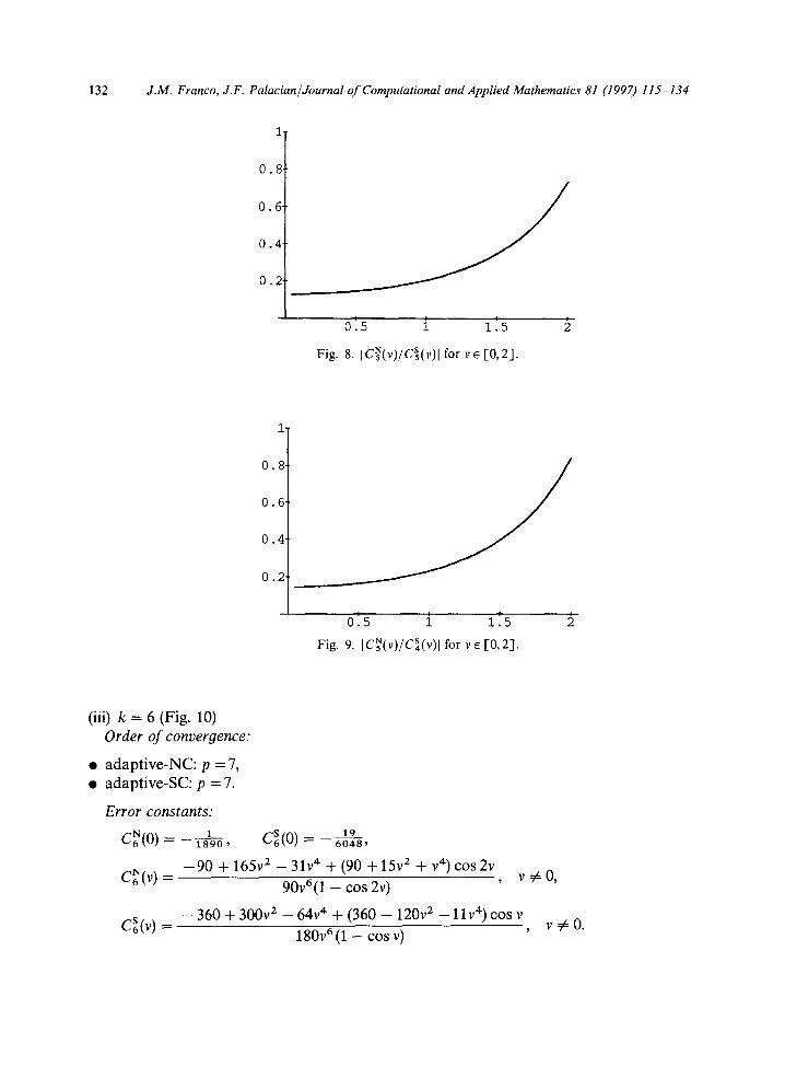
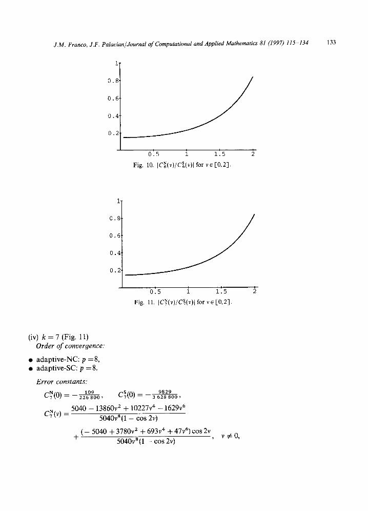
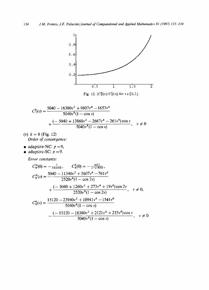
adaptive-SC methods (thereafter they will be used for numerical comparisons) with the number of steps k = 4, 5, 6, 7, 8. We denote by C~(v) the error constant of the local truncation error operator for the k-step adaptive-NC method and by cS(v) the same for the k-step adaptive-SC method. As it was expected, when v = 0 the constant coincides with the one of the constant coefficient methods. We also present some figures where we draw the absolute value of the ratio between the error constants corresponding, respectively, to the adaptive-NC and adaptive-SC methods I CkN (v)/CkS (V) I for v e [0, 2]. From these pictures one realizes that the constants C~(v) are of a smaller size than the constants CS(v). This fact was already known for the classical methods of constant coefficients and, as we shall see in Section 4, it will imply an improvement of the numerical results of the adaptive-NC methods against the adaptive-SC methods.
3. Linear stability of the methods
In this section, we study the stability of the adaptive methods when they are applied to the standard linear test method.
Definition. A multistep method, when it is applied to the linear test model y" + )~2y = 0, is said to be unconditionally stable if all the roots (j(H) of the stability polynomial (characteristic polynomial) satisfy the condition
[~j(H)I ~< 1 for all n = 2h > 0, (3.1)
and the multiple roots are I~j(H)I < 1. When condition (3.1) is satisfied for all H~(0 , V), this interval is called the stability interval of the method.

1 2 2 J.M. Franco, J.F. Palacian/Journal of Computational and Applied Mathematics 81 (1997) 115-134
Let us test the adaptive methods with the standard linear test model as given in the form
y" + o)2y = - ey, (3.2)
where e = 2 2 - e) 2 and indicates the type of approximation for which the main frequency of the problem, 2, is estimated by the parameter co. If the method (2.5) is used to solve Eq. (3.2), the numerical solution satisfies the difference equation
k
Y , + 2 - 2 ( c o s 2v)y, + y , -2 = - h2e ~ rij(v)y,,+,_j. (3.3) j = O
Denoting z = eh 2, the characteristics equation associated with the difference Eq. (3.3) can be expressed in the form
Z = - - ~ k - 2 ( ~ 2 - 2 cos 2v + ( - 2 ) / ~ k = o rij(V)( k-j. (3.4)
In order that z to take values such that the roots of (3.4) lie on the unit circle, we put ((v) = e i°, 0 ~< 0 ~< 2re into (3.4) and, after simplifications, we obtain
2(cos 2v - cos 20) f R cos (k - 2 ) 0 + S sin(k - 2 ) 0 , z(O)
= R 2 + S 2 ~ + i(R sin(k - 2 ) 0 - S cos(k -2)0) , (3.5)
where the quantities R and S represent the Fourier sums
R = rio(V)COS kO + ril(V)Cos(k - 1 ) 0 + -.- + rig(V),
S = rio(V) sin kO + ril(v) sin(k - 1)0 + ... + rig_ l(v) sin 0.
Expression (3.5) provides the equations that define the boundary of the stability region in the complex plane (boundary locus) for the adaptive-NC methods.
In a similar way, the characteristic equation and the boundary locus for the adaptive-SC methods are given, respectively, by
Z = - - ( k - 2 ( ~ 2 - 2 ( c o s v)( + 1)/~k=o rij(V)( g-j, (3.6)
2(cos v - cos 0) ~" R cos (k - 1)0 + S sin(k - 1) 0 z(O) (3.7)
R E + S 2 ~ + i(R sin(k - 1)0 - S cos(k - 1)0).
Now we analyze the properties concerning the stability of the adaptive methods for those cases of practical interest.
3.1. The main frequency o f the problem is exactly known
This occurs when the main frequency 2 is exactly equal to parameter o9, and then e = 0. In this case z = 0, and the stability polynomial (3.4) for the adaptive-NC methods reduces to
((4 --2(cos 2v)( 2 + 1)( k-4 =0, (3.8)
so that the roots are (l(V) = e iv, (2(v) = - e iv, (3(v) = e -iv, (4(v) = - e -iv, (j(v) = 0, j ~> 5. In other words, the principal roots are simple and they are on the unit circle. Besides, the spurious roots are null.
J.M. Franco, J.F. Palacian/Journal of Computational and Applied Mathematics 81 (1997) 115-134 123
Similarly, the stability po lynomia l (3.6) for the adapt ive-SC me thods reduces to
((2 - 2 ( c o s v)( + 1)( k - 2 =0, (3.9)
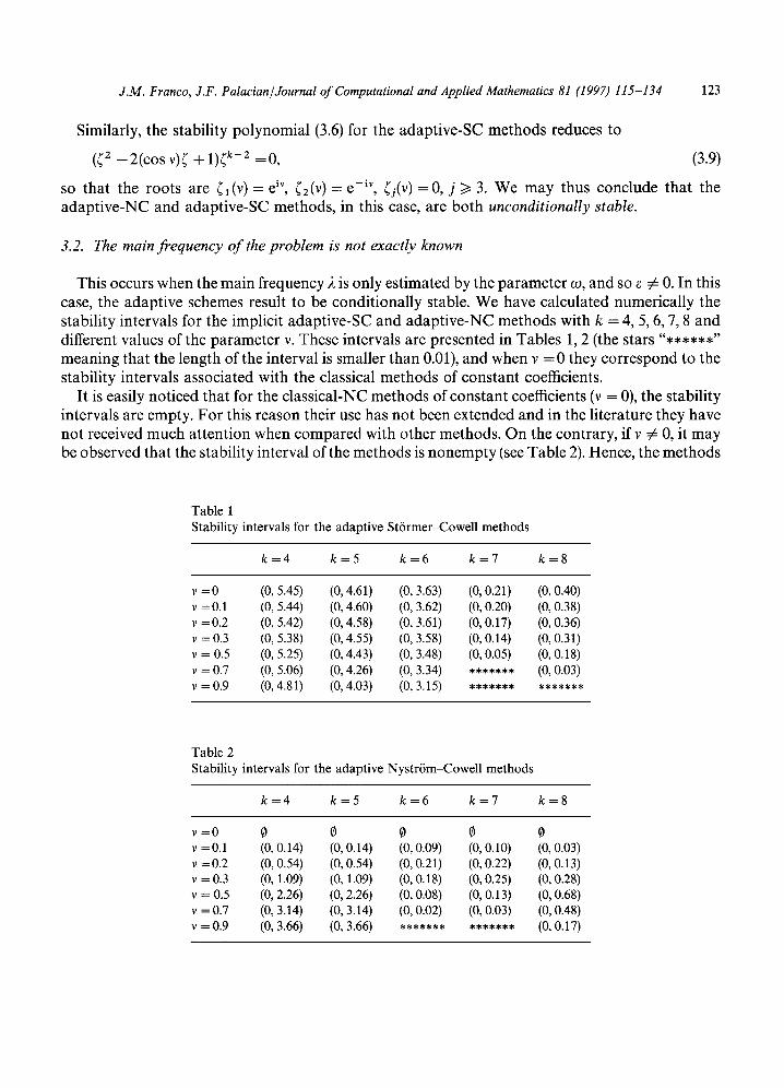
SO that the roots are ( l ( v ) = e iv, ( 2 ( v ) = e -iv, ( j ( v ) = 0 , j >~ 3. We m a y thus conclude that the adap t ive -NC and adapt ive-SC methods , in this case, are bo th unconditionally stable.
3.2. The main frequency of the problem is not exactly known
This occurs when the main f requency 2 is only es t imated by the pa rame te r o~, and so e ~ 0. In this case, the adapt ive schemes result to be condi t ional ly stable. We have calculated numer ica l ly the stability intervals for the implicit adapt ive-SC and adap t ive -NC me thods with k = 4, 5, 6, 7, 8 and different values of the pa rame te r v. These intervals are presented in Tables 1, 2 (the stars "******" mean ing that the length of the interval is smaller than 0.01), and when v = 0 they cor respond to the stability intervals associated with the classical me thods of cons tan t coefficients.
It is easily not iced that for the classical-NC me thods of cons tant coefficients (v = 0), the stability intervals are empty. Fo r this reason their use has not been extended and in the l i terature they have not received m u c h a t tent ion when c o m p a r e d with o ther methods . On the cont rary , if v :~ 0, it m a y be observed that the stability interval of the me thods is n o n e m p t y (see Table 2). Hence, the me thods
Table 1 Stability intervals for the adaptive St6rmer-Cowell methods
k = 4 k = 5 k = 6 k = 7 k = 8
v = 0 (0, 5.45) (0, 4.61) (0, 3.63) (0, 0.21) (0, 0.40) v = O. 1 (0, 5.44) (0, 4.60) (0, 3.62) (0, 0.20) (0, 0.38) v =0.2 (0, 5.42) (0, 4.58) (0, 3.61) (0, 0.17) (0, 0.36) v = 0.3 (0, 5.38) (0, 4.55) (0, 3.58) (0, 0.14) (0, 0.31) v = 0.5 (0, 5.25) (0, 4.43) (0, 3.48) (0, 0.05) (0, 0.18) v = 0.7 (0, 5.06) (0, 4.26) (0, 3.34) ******* (0, 0.03) v = 0.9 (0, 4.81) (0, 4.03) (0, 3.15) ******* *******
Table 2 Stability intervals for the adaptive Nystr6m-Cowell methods
k = 4 k = 5 k = 6 k = 7 k = 8
v=O ~ ~ 0 0 0 v =0.1 (0, 0.14) (0, 0.14) (0, 0.09) (0, 0.10) (0, 0.03) v =0.2 (0, 0.54) (0, 0.54) (0, 0.21) (0, 0.22) (0, 0.13) v = 0.3 (0, 1.09) (0, 1.09) (0, 0.18) (0, 0.25) (0, 0.28) v = 0.5 (0, 2.26) (0, 2.26) (0, 0.08) (0, 0.13) (0, 0.68) v = 0.7 (0, 3.14) (0, 3.14) (0, 0.02) (0, 0.03) (0, 0.48) v = 0.9 (0, 3.66) (0, 3.66) ******* ******* (0, 0.17)
124 J.M. Franco, J.F. Palacian/Journal of Computational and Applied Mathematics 81 (1997) 115 134
we are proposing in this paper can be considered as a stabilization of the classical NystriSm-Cowell methods that appeared in [5].
On the other hand, it is worth not ing that, for k = 4, 5, 6, the stability interval of the adaptive- NC methods is smaller than the one of the adaptive-SC methods. But this does not mean a l imitation for these methods after assuming that the problems to be solved are nonstiff and that the parameter co is a good approximat ion of the main frequency 2(e ,~ 1). Thus, the intervals we have obtained are adequate for preserving the stability of most of the real applications. For example, in the figures of Section 4, a good qualitative behaviour of the adapt ive-NC methods can be observed, even for integration steps relatively long.
4. Numerical results
To illustrate the behaviour of the methods derived in Section 2, some numerical applications for a family of test problems are shown in the following. We consider:
(i) The present methods given by (2.5) and (2.7). (ii) Adaptive St6rmer-Cowel l methods [4].
(iii) Cowell's me thod [5]. (iv) Adam's me thod [5]. using various step sizes. These methods are of mult istep type and can be obtained for arbitrary high order of approximat ion in recurrent form. We consider all the methods with order six, that is to say, they are comparable in terms of local approximat ion and computa t iona l cost. The methods are implemented in predictor-corrector form (PECE) and the initialization values are computed using an eighth-order R unge -Ku t t a me thod derived by Prince and D o r m a n d [10] with step size h/4, h being the step size used by the methods (i)-(iv).
Example 1. The quasi-periodic linear problem
Z" + fD2Z = /3f.O 2 exp(icot), t ~ [0, 1000], z ~ C
z(0) = 1, z'(0) = i(co - e/2).
Its analytic solution is given by
( ) ( ) z(t)= cos c o t + ~ t s i n c o t + i sin c o t - ~ t c o s c o t ,
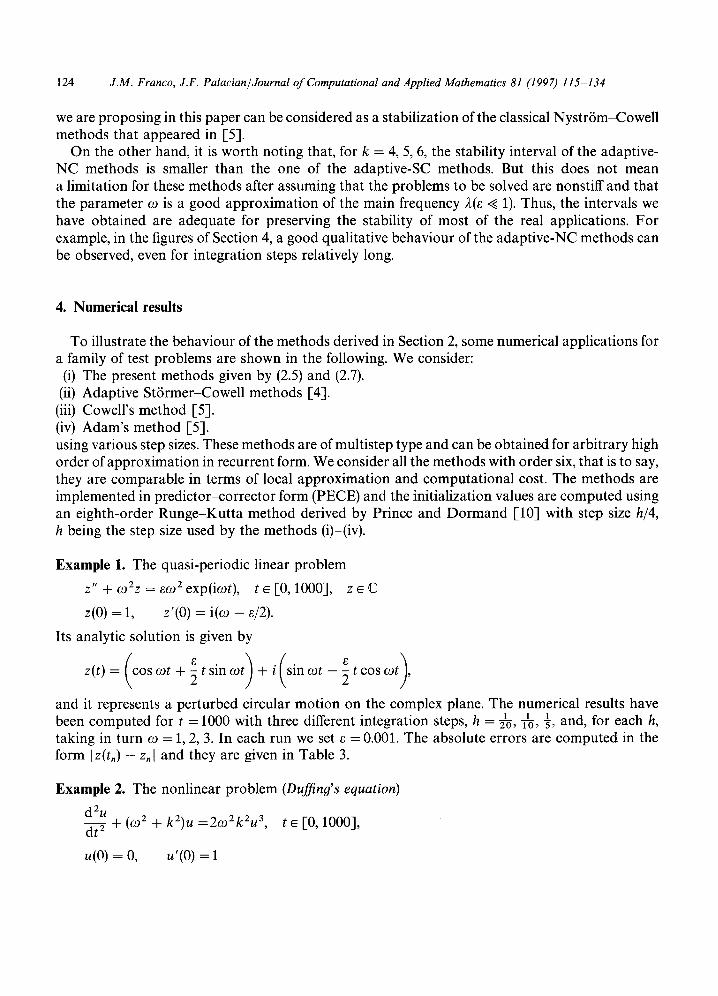
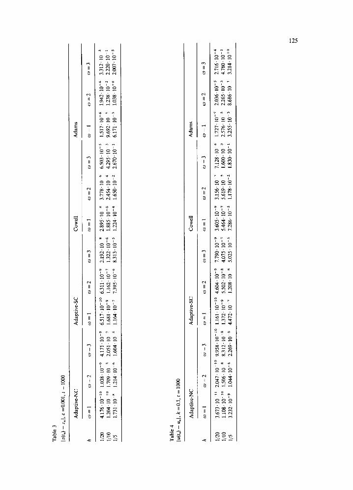
and it represents a per turbed circular mot ion on the complex plane. The numerical results have been computed for t = 1000 with three different integration steps, h - 1 1 1 2o, lo, 3, and, for each h, taking in turn co = 1, 2, 3. In each run we set ~ = 0.001. The absolute errors are computed in the form I z(t,) - z, I and they are given in Table 3.
Example 2. The nonlinear problem (Duffing's equation) d2u dt 2 + (co2 + k2)u =2co2k2u 3, t ~ [0, 1000],
u (o) = o , u ' (O) - - 1
Tab
le 3
Iz(t
,) -
z,
I, e
=0
.00
1,
t =
1000
Ad
apti
ve-
NC
A
dap
tiv
e-S
C
Co
wel
l A
dam
s
h 0
9=
1
09
=2
0
9=
3
09
=I
09
=2
0
9=
3
09
=1
0
9=
2
co=
3
o9
=1
0
9=
2
09
=3
1/20
1/10
1/5
4.1
76
"10
-l°
1.0
38
"10
-9
4.1
71
"10
9
6.5
17
"10
1o
6
.31
1.1
0-9
2
.19
2.1
0-s
2
.89
5.1
0-8
3
.77
8.1
0-6
6
.50
3.1
0-5
1
.51
7.1
0-6
1
.94
2.1
0-4
3
.31
2.1
0-3
1.2
04
"10
ao
1
.70
9"1
0
s 2
.05
1.1
0-7
1
.68
1.1
0-9
1
.16
2.1
0-7
1
.32
2.1
0-6
1
.88
5"1
0 -6
2
.45
4"1
0
4 4
.29
5.1
0-3
9
.69
2"1
0
5 1
.23
8.1
0-2
2
.22
0.1
0-1
1.73
1" 1
0 -s
1.
214"
10
-6
1.60
4" 1
0 -5
1.
164"
10
-7
7.39
5" 1
0 -6
8.
313"
10
-5
1.22
4" 1
0 -4
1.
650"
10
z 2.
670"
10
1 6.
171"
10
-3
1.03
8" 1
0 +
° 2
.00
7'
10 ÷
s
Tab
le 4
lu(t
.) -
un
l, k
=0.1
, t
=100
0
Ad
apti
ve-
NC
A
dap
tiv
e-S
C
Co
wel
l A
dam
s
h 0
9=
1
09
=2
0
9=
3
o9
=1
0
9=
2
09
=3
co
=l
09
=2
0
9=
3
09
=1
0
9=
2
09
=3
1/20
1/10
1/5
3.6
73
.10
-11
2
.04
7.1
0 -
l°
9.9
58
.10
-lo
1
.16
1.1
0 -
lo
4.6
04
.10
-9
7
.79
0-1
0 -
9
3.6
05
.10
-9
3
.15
6.1
0 -
7
7.1
28
.10
-6
1
.72
7.1
0 -
7
2.0
36
.10
-5
2
.71
6.1
0 -
4
1.10
8" 1
0 -1
° 1.
506"
10
-8
8.31
2" 1
0 -a
1.
372"
10
-9
5.50
2" 1
0 -8
4.
075"
10
7 5.
464"
10
-7
5.61
9" 1
0 -5
1.
600"
10
-3
2.57
6" 1
0 -s
2
.26
5'
10 -
3
4.76
0" 1
0 -1
3.23
2" 1
0 -8
1.
044"
10
-6
2.26
9" 1
0 -6
4
.47
2'
10 -
v
1.20
8" 1
0 6
5.02
5" 1
0 -5
7.
286"
10
-5
1.17
8" 1
0 -z
1.
830"
10
-t
3.25
5" 1
0 -3
8.
686"
10
1 3.
214"
10
+°
F_,
126 J.M. Franco, J.F. Palacian/Journal of Computational and Applied Mathematics 81 (1997) 115-134
with co > 0, 0 ~< k < co. The analytic solution is
u(t) = 1 sn(cot; k/co) (1)
and represents a periodic motion in terms of an elliptic function. We have calculated the numerical solution in t = 1000, for the integration steps h - 1 1 1 20, lo, 5, and parameter values k =0.1 and co = 1, 2, 3. The absolute errors are tabulated (in I" i-norm) in Table 4.
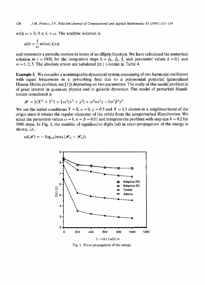
Example 3. We consider a nonintegrable dynamical system containing of two harmonic oscillators with equal frequencies in a perturbing field due to a polynomial potential (generalized H6non-Heiles problem, see [1]) depending on two parameters. The study of this model problem is of great interest in quantum physics and in galactic dynamics. The model of perturbed Hamil- tonian considered is
~--- l ( X 2 ._[_ y2) + 1(.02(X2 .~_ y2) + C02~tx2y _2co2f12y4.
We use the initial conditions Y = 0, x = 0, y -- 0.5 and X = 0.5 chosen in a neighbourhood of the origin since it retains the regular character of the orbits from the nonperturbed Hamiltonian. We select the parameter values co = 1, ~ = fl = 0.01 and integrate the problem with step size h = 0.2 for 5000 steps. In Fig. 1, the number of significative digits (sd) in error-propagation of the energy is shown, i.e.,
s d ( ~ ) = - log,o(maxl ~ o - ~,~. I)-
v
r.~5'
8
7 ~ . . . . . .
6 \ ',, . Adap, ivo-NC -~- Adaptive-SC
-e- Cowell
~ - ~ . . -N- Adams
% ..... -4- ..... .@ % %
4 % %
3 ~ . . . . . ~ . . . . . .~
0 200 400 600 800 1000
t-variable
Fig. 1. Error-propagationoftheenergy.
1200
J.M. Franco, J.F. Palacian/Journal o f Computational and Applied Mathematics 81 (1997) 115-134 127
-2
. o ° • °
• o o- o• . .
• " ° ° o o • - ! -" . . . . . . ' " . . . . . . o • . . . °
".. ".. - i //:.:•::.• . . . . . . . . . . . . . . . . . . . " . " ! • ¢ ; t ' . . . . . . . . . . . . . . . . . . . .
• " . " . , s s I 1 / ~ " - - . . . . " " •
• . " . . " . . ,,.. ~. '~ I / ' f , , ¢ , , . - . , : ' . ~ . . . • . . . . . . . • • o "o "Oo "% ,11~ ~ • ~ . Q . " - o . . • • . o
m
•. "-.. ".,....x,~ "~"t'..."., " ' , . " ". • " "%. ~"'~,.v~. ~ " ~ ' % ' " " "° " •
I m ,, ......... ..:="/..pJ~ ~ : ". ". ". • . . ~ J $ I • % ' . • o • . o . . / I -~ m ,Z ~ o . .
........ . , ' ] i ~. - ". ". " .
• • • • o , ~ • • . •
o . • o
- 4 i i i
- 4 - 2 0 2
F ig . 2. A d a m s m e t h o d (h = 0.6, c< = 0.01).
4
0,6
0,4
0,2
0,0
-0,2
-0 ,4
f
/
• ",°,°,..,%
• o " . o - " ° ° " ° " ° ' ° " . . . . . . . • ' ° . - . • " ° . q, • . ,~.%.fu o % ~ . %
, . . . . . . . . . ,,, _
/ , " \ !
/ : i ! : J / ! ° j . S ~ s"
: k
~ %% °°-~..~°°.o.•O.--''°° ; . %,
• , •.•o•
-0,6 , , , , ,
- 0 , 6 - 0 , 4 - 0 , 2 0 , 0 0 , 2 0 , 4 O,
Fig . 3. Cowell method (h = 0.9, ~ = 0.01).
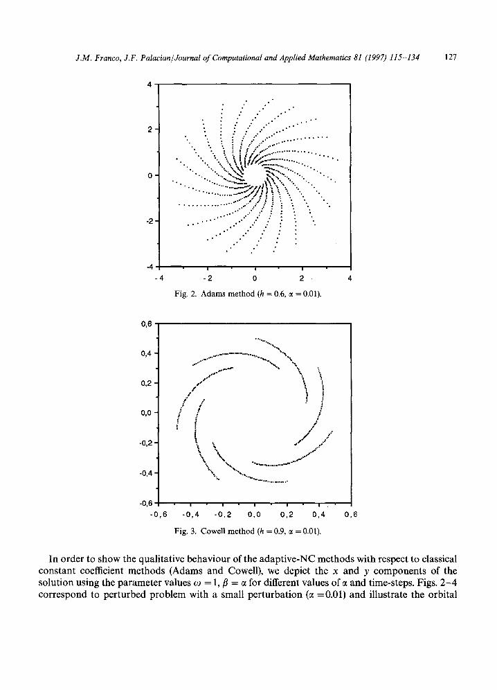
In order to show the qualitative behaviour of the adaptive-NC methods with respect to classical constant coefficient methods (Adams and Cowell), we depict the x and y components of the solution using the parameter values co = 1,/3 = ~t for different values of ~ and time-steps. Figs. 2 - 4 correspond to perturbed problem with a small perturbation (~ =0.01) and illustrate the orbital
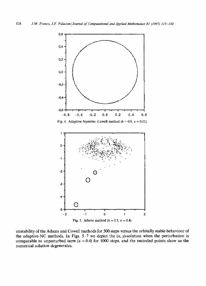
128 J.M. Franco, J.F. Palacian/Journal of Computational and Applied Mathematics 81 (1997) 115-134
0 , 6
0,4
0,2
0,0
-0,2
-0,4
,,,, / ; \o ! -
: t |
i I m
\ ,.; , / \ ,-
\ /
- 0 , 6 , , , , ,
- 0 , 6 - 0 , 4 - 0 , 2 0 , 0 0 , 2 0 , 4 0 , 6
Fig. 4. A d a p t i v e N y s t r 6 m - C o w e l l m e t h o d (h = 0.9, ~ = 0.01).
-1
-2
-3
-4
-5
• • •
• - - : . . ~ . . - . . - o . • ;-,-." ...',• ....,-.--...- .. . . . . ' - . - ; . °% • . . . .I.~1.~ . , . • • • • : : , i ' . ~ ' , ' : ' " . " 7 . . - - ~ : . . . -.-
q.. - • . ¢~ - . . . . . . . a . . . < • . : . " o ' i 'P. ~ . uv | ' . ; . • " ; J . " . ¢ ' . • .> " " : . .:-, .:...:~':..¢... f . : : - - . . p . . . - . .'- .
• • • , 8 . . . ' I - . . . . , ' - ; " ¢ . . , • . . . . : . . , : . . . .~.~.; ,. - . , : . . . ? • . • " . ; . . . . - . . . . . ".. .
E)
O
(9 g I I
- 2 -1 0 1 2
Fig. 5. A d a m s m e t h o d (h = 0.5, c< = 0.4).
unstability of the Adams and Cowell methods for 500 steps versus the orbitally stable behaviour of the adaptive-NC methods• In Figs. 5-7 we depict the (x, y)-solution when the perturbation is comparable to unperturbed term (~ = 0.4) for 1000 steps, and the encircled points show as the numerical solution degenerates.

J.M. Franco, J.F. Palacian/Journal of Computational and Applied Mathematics 81 (1997) 115-134 129
-1
-2
-3 '
.. .;.: ",%.,; =, ":.... .
= ; . . 1 , ' = ' - ' . . • . • . ' = . • . ~ - = . ' - • . . . . • ,.~.,.,,., . . , . ~. ~.~," .
. ; ,~:o~=.'g~ . . . . . . ~ . . ~:%,ff~.;,.: . • : ~ " . ¢ ' . ~ $ ~ : . . • • " " ~ ' - [ , _ ' ~ i • ¢ - •
; • - " . ~ - . * ~ i == : . • ~ . " . ~ . ~ : ==.~:. •" • " " • • ' t ; ~ . P - r " • " - . . ~ . n " : ~ ' • "
, " . • " ~ . • . : J - ~ . . m ' . . . : , . - ' 1 . : - - ~ . " . * • • . . • • , , • - u . : l w $ ~ ¢ , ~ , ' . . ~ • ~ • •
• • • , . . - . . . . ' . % - . : - " ~ . : . . - ' . . . •
Q ° . o
Q
O " 4 I I I
- 2 -1 0 1
Fig . 6. C o w e l l m e t h o d (h = 0.9, ~ = 0.04).
: " ° • . . . . o .
• -'.'~ ,.:.'..- -=,;. ~.;" .. :'-•":•°•. :" ".:v-.:, .
" 4 o ° . " ~." " . "
• " L ' - X , ~ ' l , ' : ' ~ . ' " . . - ' . . - ; , . . ; . , , ~ i - ~ = ° .
- .'qr.~ " ' • ' . ' . ; ~ . • • • • oo.¢ • • o• o • • • • • • ~
• . • . ¢ ~ . _ . . . • ~ . ~ . •
• " - - ~ _ $ / ~ : ' - , .~ * . ' ~ . " " ~ r • ' " " " • • • • . ; • . ~ . . : . , - . : • : • . , ~ • . . . .
• . . - . ' ~¢ ~ , : : . ~ ¢ - ' . - . ~ . , . •
• • • . . . , . -s • : ; . : , . . ; • • •
• •• :• ": i'-.:":"i " .'
- 2 I I I
- 2 -1 0 1
Fig . 7. A d a p t i v e N y s t r 6 m - C o w e l l m e t h o d (h = 0.9, ~ = 0.4).
5. Conc lus ions
F r o m n u m e r i c a l results presented in Tables 3 and 4 and Figs. 1 - 7 w e c o m e to the f o l l o w i n g conc lus ions :

130 J.M. Franco, J.F. Palacian/Journal of Computational and Applied Mathematics 81 (1997) 115-134
Adams methods yield poorer results than Cowell, adaptive-SC and adaptive-NC methods which are designed for second-order special equations of the form y" =f(t, y). In particular, Fig. 1 shows that the error-propagation degenerates much faster in the Adams methods.
Adaptive-NC methods are the most efficient for the test problems considered when the main frequency is known and the restoring terms represent a small perturbation. This result of better approximations by the adaptive-NC methods when compared with the adaptive-SC methods, is due to the fact that the error constants of the latter are bigger, although both types of methods have very similar properties of linear stability (orbital stability). In general, the error growth is much faster in the Adams and Cowell methods when the frequency ~o increases, and at the end of the interval of integration the size of the error is approximately greater than three orders of magnitude with respect to the adaptive-NC methods.
The behaviour of orbital stability of the adaptive-NC method is shown in Fig. 4. This method yields the right qualitative behaviour of the solution circulating around the origin, whereas the Adams and Cowell methods spiral about it. Although the time-step considered for the Adams method is smaller, it degenerates very quickly. When the perturbation is not small (~ = 0.4), the solution computed by the adaptive-NC method circulates around the origin (see Fig. 7), but it degenerates very fast when it is obtained by the other methods (see the encircled points in Figs. 5 and 6). These algorithms fail in the 860th time-step approximately by reason of a numeric overflow. Of course, the nice appearance of Fig. 7 (which shows a good behaviour of the linear stability) when compared with Figs. 5 and 6 does not guarantee that the computed points are close to the corresponding values of the theoretical solution because the integration steps are very large. Undoubtedly, the adaptive-NC scheme have identified the right qualitative behaviour and this was the point of interest in these experiments.
The paper is limited to one positive eigenvalue; we intend to extend the method for the case of large second-order ODEs systems in the context of semidiscretized second-order hyperbolic equations. In these problems, there will appear a symmetric positive definite matrix (stiffness matrix) that contains implicitly the frequencies of the problem.
Acknowledgements
This work was supported in part by Project P IT-13/90 of the Diputaci6n General de Arag6n. We are thankful to A. Deprit for helping us in preparing the manuscript.
References
[1] A. Abad, A. Deprit, A. Elipe and M. Sein-Echaluce, A perturbed elliptic oscillator: flow inversion through butterfly bifurcations, Rev. Acad. Cienc. Zaragoza 44 (1989) 89-105.
[2] J.M. Correas, Linear Multistep Schemes based on algebraic, trigonometric and exponential polynomials, Proceed- ings of the First World Conference on Mathematics at the Service of Man, vol. 1, Universidad Polit6cnica de Barcelona (Spain), 1977, pp. 339-359.
[3] J.M. Correas, M.C. Martin, M~todos multipaso de coefficientes variables para el P.V.I. 2 especial, V-Jornadas Mat. Luso-Espafiolas, Universidad de Aveiro (Portugal). 3 (1978) 940-962.
J.M. Franco, J.F. Palacian/Journal of Computational and Applied Mathematics 81 (1997) 115-134 131
[4] J.M. Franco, J.M. Correas, Mrtodos de tipo St6rmer-Cowe11 con coefficientes variables. Applicationes a la integraci6n de movimientos orbitales, Actas del X-CEDYA, Universidad Politrcnica de Valencia 1 (1987) 117-124.
['5] P. Henrici, Discrete variable methods in ODE's, Wiley, New York, 1962. ['6] M.K. Jain et al., P-stable methods for periodic I.V.P. of second order differential equations, BIT 19 (1979) 347-355. ['7] U. Kirchgraber, An ODE-solver based on the method of averaging, Numer. Math. 53 (1988) 621-652. 18] B. Neta, C.H. Ford, Families of methods for ordinary differential equations based on trigonometric polynomials. J.
Comput. Appl. Math. 10 (1984) 33-38. 1-9] M. Palacios, J.M. Franco, Adaptive Cowell methods for orbital motions, in: J. Teles (Ed.), Orbital Mechanics and
Mission Design, Proceedings of AAS/NASA, vol. 69, AAS Publications Office, San Diego, California 92128, 1989, pp. 3-22.
[10] P.J. Prince, J.R. Dormand, High order embedded Runge-Kutta formulae, J. Comput. Appl. Math. 7 (1981) 65-75. [-1 I] E. Stiefel, D.G. Bettis, Stabilization of Cowell's methods, Numer. Math. 13 (1969) 154-175.
Appendix. Error constants of the implicit adaptive N C and SC methods
I n th is a p p e n d i x we p r e s e n t t he loca l t r u n c a t i o n e r r o r c o n s t a n t s fo r t he imp l i c i t N y s t r S m - C o w e l l m e t h o d s ( d e n o t e d b y C~(v)) a n d fo r the imp l i c i t S t 6 r m e r - C o w e l l m e t h o d s ( d e n o t e d b y CS(v)). I n a d d i t i o n , fo r e a c h o r d e r , we c o m p a r e b o t h e r r o r c o n s t a n t s b y m e a n s o f t he a b s o l u t e v a l u e o f the
q u o t i e n t b e t w e e n t h e m , fo r t yp i ca l v a l u e s o f v, i.e. v v a r y i n g f r o m 0 to 2.
(i) k = 4 (Fig. 8) Order of convergence:
• a d a p t i v e - N C : p = 6 , • a d a p t i v e - S C : p = 5.
Error constants."
c (o) c (o) = - - 1 8 9 0 , - - 2 4 0 ,
C~(v) = - 9 0 + 165v 2 - 31v 4 + (90 + 15v 2 + v 4) cos 2v
90v6(1 - cos 2v) , v :/: 0,
CS(v ) = 12 - 5v 2 - (12 + v 2) cos v 12v4 ( 1 - cos v) , v ~ 0 .
k = 5 (Fig. 9)
Orders of convergence:
a d a p t i v e - N C : p = 6 , a d a p t i v e - S C : p = 6.
Error constants:
c (o) -
(ii)
1 CS(O) 1 8 9 0 ~ = - - 6 0 4 8 0 ~
C~(v) = - 9 0 + 165v 2 - 31v 4 + (90 + 15v 2 + v 4) cos 2v 90v6(1 - cos 2v) , v ~ 0,
c (v) = - 360 + 480v 2 - - 139v 4 + (360 - - 300v 2 - - 2 6 v 4) cos v
360v 6 (1 - - cos v) , v ~ 0.
132 J.M. Franco, J.F. Palacian/Journal of Computational and Applied Mathematics 81 (1997) 115-134
1 "
o.8!
0 . 6
0.4
0.2
o'.s { 1.'s i
Fig. 8. IC~(v)/CS(v)l for v e [0 ,2] .
1
0.8
0.6
0.4 i
0.2~
o's i i i • '.S
Fig. 9. [C~(v)/CS(v)] for ve [0,2].
(iii) k = 6 (F ig . 10)
Order o f convergence."
• a d a p t i v e - N C : p = 7,
• a d a p t i v e - S C : p = 7.
Error constants."
c ~ ( o ) 1 = - - 1 8 9 0 ,
C~(v) =
C~(v ) =
c ~ ( 0 ) = 19 - - 6 ~ - 8 ,
- 9 0 + 165v 2 - 3 1 v 4 + (90 + 1 5 v 2 + v 4) c o s 2 v
90v6(1 - c o s 2v) , v # O,
- 3 6 0 + 300v 2 - 64v 4 + (360 - 120v 2 - l l v 4) c o s v
180V 6 (1 - - c o s v) , v # 0.
J.M. Franco, J.F. Palacian/Journal of Computational and Applied Mathematics 81 (1997) 115-134 133
l '
0.8
0.6
0.4
0.2
i ' 5 o5 { 1.
Fig. 10. IC~(v)/CS(v)l for v e [0,2] .
1
0.8
0.6
0.4
0 . 2 -
F ig .
'5 i' o . { . 5
11. [C~(v)/Cs(v)[ for v e [0,2].
(iv) k = 7 (Fig. 11) Order of convergence:
• a d a p t i v e - N C : p = 8, • a d a p t i v e - S C : p = 8.
Error constants:
c~(o) -
C ~ ( v ) =
lo9 CS(0) 982~ 2 2 6 8 0 0 ~ = - - 3 6 2 8 8 0 0
5040 - 13860v 2 + 10227v 4 - 1 6 2 9 v 6
5040v8(1 - cos 2v)
( - 5040 + 3780v 2 + 693v 4 + 47v 6) COS 2v
4 5040v8(1 - cos 2v) , v # O ,
134 J.M. Franco, J.F. P alacian /Journal of Computational and Applied Mathematics 81 (1997) 115-134
1
0 . 8
0 . 6
0 . 4
0.2-
~5 o i l'.s
Fig. 12. IC~(v)/CS(v)l for v~ [0,2].
CS(v) = 5 0 4 0 - - 1 6 3 8 0 v 2 + 9 8 0 7 v 4 - - 1657v 6
5040v8(1 - - c o s v)
( - - 5 0 4 0 + 1 3 8 6 0 v 2 - - 2 6 6 7 v 4 - - 261v 6) c o s v
+ 5 0 4 0 v 8 ( 1 - - c o s v) '
(v) k = 8 ( F i g . 12)
Order of convergence."
• a d a p t i v e - N C : p = 9,
• a d a p t i v e - S C : p = 9.
Error constants."
c ~ ( o ) - - 1 6 2 0 0 ,
C~(v ) =
C~(v) =
C~(O) 407 - - 1 7 2 8 0 0
5 0 4 0 - - 1 1 3 4 0 v 2 + 5 6 0 7 v 4 - - 7 6 1 v 6
2 5 2 0 v 8 ( 1 - c o s 2v)
( - 5 0 4 0 + 1260v 2 + 273v 4 + 1 9 v 6 ) c o s 2 v
+ 2 5 2 0 v 8 ( 1 - c o s 2 v ) '
1 5 1 2 0 - - 2 3 9 4 0 v 2 + 10941v 4 - - 1 5 4 1 v 6
5040v8(1 - - c o s v)
( - - 1 5 1 2 0 - - 1 6 3 8 0 v 2 + 2 1 2 1 v 4 + 2 3 3 v 6) c o s v
5 0 4 0 v 8 ( 1 - - c o s y )
v ~ 0
v # O ,
, v ~ O .