Adaptive Design Methods for Checking Sequences
43
SU-SEL-72-034 Adaptive Design Methods for Checking Sequences b Y Raymond T. Boute July 1972 Technical Report No. 30 This work was supported by the National Science Foundation under Grant GJ-27527 DIGITR~ svsrEm5 MIBORRTORV 5TRllFORD ELECTROIII~S LRBORRTORlEs STRRFORD URlUERSlTV . STARFORD, CRllFORRlR
Transcript of Adaptive Design Methods for Checking Sequences
SU-SEL-72-034
Adaptive Design Methods
for Checking Sequences
bY
Raymond T. Boute
July 1972
Technical Report No. 30
This work was supported by theNational Science Foundation underGrant GJ-27527
DIGITR~ svsrEm5 MIBORRTORV
5TRllFORD ELECTROIII~S LRBORRTORlEsSTRRFORD URlUERSlTV . STARFORD, CRllFORRlR

SEL-72-034
ADAF'TIVE DESIGN METHODS FOR CHECKING SEQUENCES
bY
Raymond T. Boute
July 1972
Technical Report No. 30
DIGITAL SYSTEMS LABORATORYDepartment of Electrical Engineering Department of Computer Science
Stanford University
Stanford, California
Research reported in this paper was supported by the National ScienceFoundation under grant GJ 27527, and while Mr. Boute was partiallysupported by the Nationaal Fonds voor Wetenschappelijk Onderzoek ofBelgium.


Adaptive design methods for checking sequences
bY
Raymond T. Boute
Digital Systems LaboratoryDepartment of Electrical Engineering
Stanford University
ABSTRACT
The length of checking sequences for sequential machines can be
considerably reduced if, instead of preset distinguishing sequences, one
uses so-called "distinguishing sets" of sequences, which serve the same
purpose but are generally shorter. The design of such a set turns out to
be equivalent to the design of an adaptive distinguishing experiment, *
though a checking sequence, using a distinguishing set, remains essentially
preset. This property also explains the title.
All machines having preset distinguishing sequences also have
distinguishing sets. In case no preset distinguishing sequences exist,
most of the earlier methods call for the use of locating sequences, which
result in long checking experiments. However, in many of these cases, a
distinguishing set can be found, thus resulting in even more savings in
length.
Finally, the characterizing sequences used in locating sequences can
also be adaptively designed, and thus the basic idea presented below is
advantageous even when no distinguishing sets exist.
* BY "experiment" we mean the application of sequence(s) to the machine
while observing the output. In some instances, the words "experiment"
and " sequence" can be used interchangeably.


ii
TABLE OF CONTENTS
Abstract
Table of Contents
List of Figures
List of Tables
Introduction
Preset Distinguishing Sequences and Distinguishing Sets
Preset Distinguishing Sequences for Chetiking Experiments
Distinguishing Sets
Examples
Conclusion
References
Page
i
ii
iii
iv
1
4
5
10
21
30
31


iii
LIST OF FIGURES
1 Design of preset distinguishing sequences for Ml -
2 Design of a distinguishing set for Ml
3 Optimal choice for a distinguishing set
4 Design of a distinguishing set for M2
page
8
17
19
27

iv
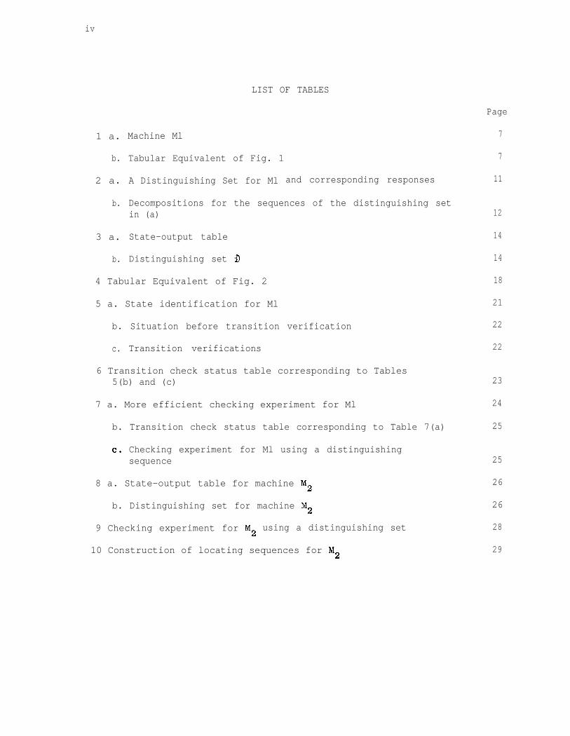
LIST OF TABLES
1 a. Machine Ml
b.
2 a.
b.
3 a.
Tabular Equivalent of Fig. 1
A Distinguishing Set for Ml and corresponding responses
Decompositions for the sequences of the distinguishing setin (a)
State-output table
b. Distinguishing set 9
4 Tabular Equivalent of Fig. 2
5 a. State identification for Ml
b. Situation before transition verification
c. Transition verifications
6 Transition check status table corresponding to Tables5(b) and (c)
7 a. More efficient checking experiment for Ml
b. Transition check status table corresponding to Table 7(a)
C. Checking experiment for Ml using a distinguishingsequence
8 a. State-output table for machine M2
b. Distinguishing set for machine M2
9 Checking experiment for M2 using a distinguishing set
10 Construction of locating sequences for M2
Page
7
7
11
12
14
14
18
21
22
22
23
24
25
25
26
26
28
29


I. INTRODUCI'ION
The concept of "experiments" on sequential machines [l) has led to
methods for checking certain classes of machines against faults [2,4,>].
For strongly-connected (an essential requirement) and reduced (a simplifying
condition) machines, checking experiments consist, in principle, of three
parts:
(1) A synchronizing [2,3] sequence or, if none exists, a homing
sequence followed by an appropriate sequence to bring the machine
in a given initial state. This latter sequence depends on the
state at the end of the homing sequence, and is thus always
adaptive.
(2) Identification of the states by means of distinguishing or, if
none exist, locating sequences. This is essentially based on
the assumption that no fault can increase the number of states*
of the machine.
(3) Checking the transitions out of each state, again including
identification of the next states.
Most often (2) and (3) are not really separate parts, but are designed
together: state identifications and transition checks are performed
together in the checking sequence whenever doing so might shorten the
final result.
Usually, the distinguishing or locating sequences used for state
identification in a checking experiment are designed as preset [3]
* Otherwise the procedure is more complicated and requires much longer
checking experiments.

2
experiments. Although a checking experiment is essentially preset (i.e.
apart from the initialization, in case no synchronizing sequence exists),
it is possible to replace the single distinguishing sequence, that is used
for the identification of every state, by a well-chosen set of sequences,
each of which is "adapted' to the state that is being identified. It
turns out that the design of such a distinguishing set is equivalent to the
design of an adaptive distinguishing experiment [3].
The sequences in a distinguishing set are nearly always shorter, and
never longer, than the shortest preset distinguishing sequences. Since
state identifications have to be done very frequently during a checking
experiment, this results in considerable savings in the number of input
symbols in the checking sequence.
Furthermore, there are many machines that have no preset distinguishing
sequence but for which a distinguishing set can be found. For such machines,
the use of a distinguishing set eliminates the need for (usually very long)
locating sequences and thus results in even more important reductions in
length. The possibility of constructing short checking experiments for
machines with adaptive distinguishing sequences has been anticipated by
I. and Z. Kohavi in [7], although they did not further explore the under-
lying principles and the practical design aspects.
In section II, we recall the basic ideas regarding preset distinguishing
sequences for later comparison with the use of distinguishing sets. We then
define the concept of "distinguishing sets" in a rigorous fashion and prove
that they can be used instead of preset distinguishing sequences. A simple
design procedure is presented and the similarities and differences with the
design of adaptive distinguishing experiments are pointed out, as well as
the advantages over distinguishing sequences. Finally, in section III, we

3
show by means of examples how to implement these ideas in designing checking
experiments. The use of a transition check status table allows additional
short cuts in an algorithmic fashion, while in the past short cuts were
found in a rather "ad hoc" fashion. The use of a distinguishing set turns
out to allow more "telescoping" than distinguishing sequences.

4
I I . PRESET DISTINGUISHING SEQUENCES AND DISTINGUISHING SETS
In this section we explain the basic ideas leading to the replacement
of preset distinguishing sequences by distinguishing sets. The reader will
soon realize that the design of distinguishing sets is equivalent to the
design of adaptive distinguishing experiments, which are discussed in
detail by Hennie [j].
First we introduce some notation and basic definitions.
Notation
We denote a sequential machine M as follows [63: M=<I,O,Q,G,h> where
I, 0, Q are respectively the input, output and state sets, 6: QXI-+Q the
next-state function and X: &x1-+0 (or Q+O for Moore machines) the output
function. Further, I*= I+U(A), where If is the set of nonempty finite
sequences of symbols from I and A is the empty sequence. Finally, we
extend 6 and h in a natural way to sequences:
6 : &XI*&, where 6(q,x) is the final state of the machine, started
in q and driven by input sequence ';;.
1 : QxIJho*, where x(q,x) is the response of the machine to ';; when
started in state q. For Moore machines: r;:QXI++O+.
Convention: 6(q,A)=q. Also x(q,A)=A for Mealy and X(q,A)d[q) for Moore
machines.
A preset distinguishing sequence for a machine M is a sequence x E I*
such that x(q,x)=T;(q',';;) implies q=q'.
In other words, the machine responds differently to x for each initial
state.
Only reduced machines -- but not all of them -- have distinguishing
sequences. However, all reduced machines have characterizing sets [2,3].

A characterizing set for a machine M is a finite subset ccI* such
that ~(q,~)=~(q' ,G) for all Z E e implies q=q'.
Usually, in case no distinguishing sequence exists, state identification
is accomplished by locating sequences, as explained in [2]. A locating
sequence (for a given state) is built from characterizing sequences and
includes repetitions to ensure that the circuit is in the same state each
time a new characterizing sequence is introduced for identifying that state.
We will not discuss this subject in detail, since characterizing sets can
be re.defined(and used)in essentially the same way as distinguishing sets
(to be defined later).
A.
qzq’
Preset Distinguishing Sequences for Checking Experiments
Definition: For every x c I*, define a partition fl: on Q as follows:
(3~) iff ?;(q,X)=X(q',G).
From the preceding definitions we immediately deduce the following
lemma:
Lemma: -x is a (preset) distinguishing sequence iff fi;; = 0 (i.e. each
block is a singleton).
This lemma leads directly to a design procedure [3] which we explain
here for later comparison with the design of distinguishing sets.
Design of Preset Distinguishing Sequences
We construct a tree-like directed graph, starting with nA and proceeding
level by level. The vertices are partitions of the form q. Each 5 gets
either 111 successors, namely the partitions s-. as i ranges over I, orXl
none at all: we do not introduce successors for Z; in case a partition
equal to Y? has already been encountered before, during the construction ofX
the tree. In this fashion, repetitions are avoided and the procedure
terminates after a finite number of steps.

6.
Distinguishing sequences -- if any exist -- are then represented by
paths leading from xn to some zero-partition,
For implementation it is easier to represent blocks of partitions 7c~;
by their state transformations under G, i.e. if (q1' q2,"' kq ] is a block
of 5, it will be represented by the block [~(ql,~),...,6(s,,~)) during
the procedure. This representation is adequate for deciding whether or not
we reached a partition 5~3; = 0, provided no merges occur for the sequence 2.
By a merge we mean that, for some 2 states ql # q2, we have x!ql,x)~(q2,~)
and 6(ql,x)=6(q2,G). But since such sequences can never be an initial part
of a distinguishing sequence, the corresponding paths in the graph are
terminated as soon as a merge is observed. This is very easy to do when
using the representation just described, since then two different states,
e.g. 6(q,G) and &(q',';;) are in the same block iff F(q,T)z(ql,r). If some
next input (after x) leads to a merge, this is immediately detected, and
for such an input no edge will leave that block.
The advantages of this representation become apparent in the following
example.
Example
For machine M1, whose state-output table is given by Table l(a), the
design graph for preset distinguishing sequences is shown in Fig. 1. The
tabular equivalent, which is more practical for computer implementation is
given in Table l(b). The three shortest distinguishing sequences are:
100, 101, 110.
Blocks containing only 1 state are not represented. In case all
blocks are singletons (i.e. "cs; = 0 and x is a distinguishing sequence) an
asterisk is written.

7
TABLE1
(a) Machine M,
input x1
D/l
D/O
Ml
B/O
6 (%X)/h hx)
(b) Tabular Equivalent of Fig. 1
inputsequences
blocks to besplit
i
0
input blocks to be inputsequences split 0 1
nn ABCDABCD -me AD,BD
11 AD,BDAD,BD ABAB BD
1010 ABAB ** *
1111 BD ** BDBD

8
ABCDy \-
(A,C merge) AD, BDO/ \
1/
AB BD
Figure 1. Design of preset distinguishing sequences for Ml.

Application to Checking Sequences
Since the design of checking sequences is discussed by Hennie [2] we
will emphasize here only the role of distinguishing sequences. This
discussion is necessary in order to justify later on their replacement by
distinguishing sets.
We assume here that the good machine has a distinguishing sequence.
Let N be the number of states. We also assume that no faulty machine can
have more than N states. (property 1)
A checking sequence is always designed in such a way that, after the
initialization part, the machine under test would be in a predetermined*
state go , in case it were the good machine. (vw=-ty 2)
The checking part itself is constructed in such a way that it would
take the good machine, started in go, at least once through each of its N
states, and identify each of these states by means of the same
distinguishing sequence 2 (yielding N different responses, by definition).
This allows to make the following conclusions for the machine under
test, depending on its response to the checking sequence:
( >1 if the response is incorrect, the machine must be faulty,
because of property 2.
( >2 if the response is correct, we have obtained N different
responses to the same sequence. Together with property 1, this
implies that there are exactly N (nonequivalent) states. This
further implies that, in case the same response to the
* In this way, only one checking experiment has to be designed. Other-
wise, one would need several ones depending on the outcome of the
initialization.

10
distinguishing sequence x is obtained at different points of the
experiment, the circuit under test must have been in the same
state each time.
The last statement in (2) forms the basis for the verification of
state transitions, since we can now identify each state unambiguously by
means of the distinguishing sequence f;.
B. Distinguishing Sets
Our main purpose is here to replace the distinguishing sequence used
to identify the states by a set of sequences that are individually designed
for each state to be identified. The following scheme is not the most
general solution possible, but seems to be the easiest to design and
implement.
The initialization of the checking experiment is done in exactly the
same fashion as explained before. Thus point (1) above is still valid.
If we also want to obtain conclusions similar to (2), based solely* on
observing the appearance of each sequence (possibly different for each
state) from the distinguishing set 9, together with a correct response, we
can proceed as follows.
Definition: A distinguishing set 9 for a machine M with state set Q
is a set of input sequences Xi, one for each qi E Q, such that for every
pair of (different) states qi, q. c Q we can write:J
-x.=u y1 ij ijT; =i;j
zij ij
* This is one of the restrictions that make this scheme not the most
general one possible.

11
where the sequences Gij' C I* are such that ~(qi,~ij)fi(q.,~..).J 13Remark: The double subscripts ij in the above definition emphasize
the fact that the decomposision of ';;i and zj
into u's, yls, etc. may depend
on both qi and q..3It is also easy to see that, for Mealy machines, the
definition implies that the first input symbol be the same for all xi C a.
This observation is the first step toward the design procedure described
below.
Example
For the machine of Table 1, a distinguishing set is given in Table 2(a).
Further, in Table 2(b) we show the decomposition into i,y,z's.
TAJ3J.3 2
(a) A Distinguishing Set for Ml and corresponding responses:
state input response final state
q xqc rD wlFq) 6 (q,xq)
A 11 10 B
B 10 00 A
C 11 11 D
D 10 01 C
I

12
(b) Decompositions for the sequences of the distinguishing set in (a):
B C D
bb0 11, A, A
w-w V,l
l,l,O w-w
10, A, A 19% 1
b 190
10, A, A
1,190
u,y zij ij' ij
Theorem. Let 3 be a distinguishing set.
If the machine under test responds to a given application of xi E 9
(at the input) by x(si,"i> and to xj E 3 by x(sj,xj), then the states
before these applications must be different (assuming qi#qj).
Proof. We denote by XT the %-function for the machine under test.
Let the states of the machine under test be q resp. q' before application
of 5;i req. X..J Then xT(q,xi)=x(qi, Fi) and ~T(q',~j)=~(qj,xj). By
definition, there exists a common initial part iij of iii and 2
3such that
'(qi,'ij)iT;(sj';;ij)' Therefore ~T(q,'ij)f7;,(q','ij) implying 424'0
Q.E.D.
Corollary
If an experiment is constructed using the same algorithm as for
designing checking experiments, except for the fact that each state qi is
identified by the corresponding xi c 3 rather than by a fixed distinguishing
sequence, then the result is a checking experiment.

13
Proof. In case the machine under test responds incorrectly to the
experiment, it is known to be faulty. In case it responds correctly, each
xi E 9 has appeared at least once (with its correct response). Therefore
we know by the preceding theorem that there must be at least N different
states. Since, by assumption, we have at most N states, the arguments
given for the checking experiments using a distinguishing sequence carry
through.
Q.E.D.
Remark
A distinguishing set should not be confused with a compound
distinguishing sequence [>] which is defined as a set of input sequences
c = (X1,X2,. . . , ",I having a common prefix ';; but otherwise unrestricted, with
the following properties:
( >1 For each block B of 'II- there is an 5;Y i 6 c that distinguishes the
states in B (i.e. given q,q' E B then x(q,xi) = x(q',xi) implies
q =q � ) l
(2) The deletion of any sequence from e will leave some states in
some block B in n- c c.Y
not distinguished by any xiAlthough the definitions are completely different, we have observed
that for machines with only a few (up to 4) states a distinguishing set 'D
satisfies at least property (1) in the above definition. This phenomenon
is purely coincidental, due to the small size of the partition blocks (this
can be verified by trying a couple of examples). However, consider now a
machine with more states, such as in Table 3(a). A distinguishing set is
shown in Table j(b).

14
5x-The longest common prefix is 1 and rc1 = ?%, ACDE and the shortest
sequence to distinguish all states of ACDE is 1111 (or 1100). Thus no
sequence 'f; i c 9 can split up this block and $) is therefore not a compound
distinguishing sequence.
TABLE 3
To illustrate the difference between a distinguishing set and
a compound distinguishing sequence
(a) State-output table (b) Distinguishing set9
state q l- 0input
D/O
B/l
B/l
c/o
B/l
A/O
B/l
A/O
D/l
F/l
C/l
E/O
Construction of a distinguishing set
state q ';;q
A 110
B 10
C 111
D 110
E 111
F 10
response
100
00
110
101
111
01
Now we show that the construction of a distinguishing set is similar
to the design of an adaptive distinguishing experiment [3].
* It is easily seen that, the longer 7, the smaller the blocks of z-+ and
the more possibility to satisfy property (1) of a C-set.
15
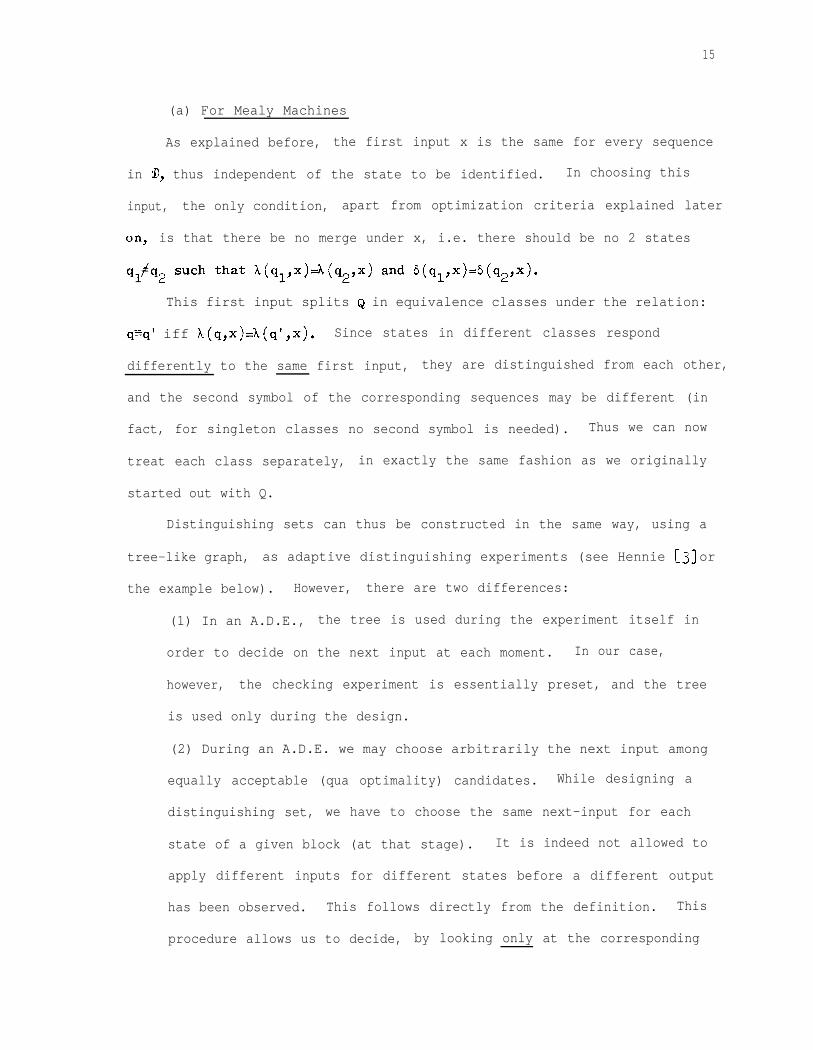
(a) For Mealy Machines
As explained before, the first input x is the same for every sequence
in 3, thus independent of the state to be identified. In choosing this
input, the only condition, apart from optimization criteria explained later
On, is that there be no merge under x, i.e. there should be no 2 states
qlfs2 such that i(ql,x)a(q2,x) and 6(sl,x)=6(s29x)m
This first input splits Q in equivalence classes under the relation:
q=q' iff h(q,x)=A(q',x). Since states in different classes respond
differently to the same first input, they are distinguished from each other,
and the second symbol of the corresponding sequences may be different (in
fact, for singleton classes no second symbol is needed). Thus we can now
treat each class separately, in exactly the same fashion as we originally
started out with Q.
Distinguishing sets can thus be constructed in the same way, using a
tree-like graph, as adaptive distinguishing experiments (see Hennie [3] or
the example below). However, there are two differences:
(1) In an A.D.E., the tree is used during the experiment itself in
order to decide on the next input at each moment. In our case,
however, the checking experiment is essentially preset, and the tree
is used only during the design.
(2) During an A.D.E. we may choose arbitrarily the next input among
equally acceptable (qua optimality) candidates. While designing a
distinguishing set, we have to choose the same next-input for each
state of a given block (at that stage). It is indeed not allowed to
apply different inputs for different states before a different output
has been observed. This follows directly from the definition. This
procedure allows us to decide, by looking only at the corresponding

i16
sequences from 9 and their responses, whether the states are, in
fact, different.
( >b For Moore Machines
The procedure is completely analogous. The only difference is that
before the application of the first input (i.e. we apply A) we can already
split Q into equivalence classes, since X is a map Q+O.
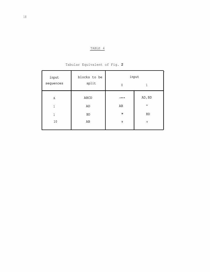
Example
Fig. 2 represents the design graph for machine Ml (see Table l), and
Table 4 its tabular equivalent.
As before, we represent the blocks by the successors of the initial
states as we trace our path along the graph. Singletons are not
represented. The symbols between parentheses represent the output
corresponding to each block, except for single blocks. Table 2(a)
represents the distinguishing set having the shortest sequences.
Optimal Choice of a Distinguishing Set
This can be done in exactly the same way as choosing the optimal
next-input during an adaptive distinguishing experiment [3]. To recall
briefly: assign a number to each block in the graph, starting with zero's
for singletons. Assign the predecessor numbers according to the following
formulae:
n = min(y, m2,...nj)
m. =3
max(n. ,Jl '*+%
>+l
The symbols are explained in Fig. 3. Clearly those numbers give, for each
block, the length of the shortest sequence for distinguishing a given state
in that block, assuming the worst chaise regarding that state. For more
details we refer to Hennie [3].

Y 1
0\ / 0” -
18
TABLE 4
Tabular Equivalent of Fig. 2
44
inputinput blocks to beblocks to be inputinput
sequencessequences splitsplit 00 11
AA ABCDABCD W-MW-M AD,BDAD,BD
11 ADAD ABAB **
11 BDBD ** BDBD
1010 ABAB ** 3636

r=jd -.
d
20
Comparison with (Preset) Distinguishing Sequences
In designing distinguishing sequences, we have to refine partitions,
while the design of distinguishing sets consists of splitting up the blocks
of these partitions separately. The significance of this observation can
be appreciated by comparing the construction of the corresponding graphs.
The main consequences are:
-- the longest sequence in an optimal distinguishing set is at most as
long as the shortest preset distinguishing sequence.
-- since it may be the case that certain blocks cannot be split up
simultaneously by any single sequence while allowing refinement by
separate sequences, distinguishing sets may exist where no
distinguishing sequences can be found.

21
III. EXAMPLES
( >a Checking Experiment for M1Initialization: the shortest synchronizing sequence for Ml is 0101
and brings the machine in state D.
Checking part. We first illustrate the design of the checking part
with separate state identification and transition checking. State
identification is done as follows (use Table 2(a)).
- Identify starting state D by xD = 10
This brings us in state C.
- Identify C by 11. New state: D.
- Go from D to A by input 0.
- Identify A by 11. New state: B.
- Identify B by 10. New state: A.
The resulting sequence, together with its response, is given in Table ?(a).
If the machine under test responds correctly, we know the states q1'92'93,44
are different (see central theorem, section II).
TABLE j(a): State identification for Ml.
1 0 1 1 0 1 1 1 0 input
q1 q2 q3 q4 state
0111c1000 output
We denote these states by the corresponding names borrowed from the good
machine (resp. D, C, A, B). Since we assume that the machine under test
has at most 4 states, it must now be in one of the states already
encountered. If it were the good machine it would be state A. By means of

22
xA = 11 we verify for the machine under test that it is indeed in the state
we decided to call A. The new situation is shown in Table 3(b).
2(b):TABLE Situation before transition verification.
1 0 1 1 0 1 1 1 0 1 1 (input)
D C A B A (state)
0 1 1 1 0 1 0 0 0 1 0 (output)
Now we are ready for the transition verification. From Table 3(b) it
is clear that the machine under test is in state B since 6(A,ll) = B has
been verified.
We check now the transition out of this state under input 1 (on the left
side of Table 3(c)) by means of x,, = 10 (we know we should use T,., byJJ
referring to the good machine).
TABLE 5k): Transition verifications.
1 1 0 1 1 1 0 1 1 0 1
B D C A B C A
0 0 1 1 1 0 1 1 1 0 1
( >1 (31 (4) (5)
u
1 0 0 1 0 0 1 0 1 1
D C B A B A D
0 1 0 0 0 0 0 0 1 0
(6) (7) (8 >
1 0
B
0 0
Note here that 6(B, 10) = A and 6(B,l) = D (just verified) now automatically
verifies 6(D,O) = A (see (2), Table 3(b)).
We proceed in this manner until all transitions have been verified.
Table 2(c) completes the sequence. The numbers correspond to the order in
which the transitions are verified, while Table 6 allows us to keep track

23
of these verifications (and see which check to do next). In practice one
does not put numbers in such a "transition check status table" but only
check marks, as the design goes along.
TABLE 6
Transition check status table corresponding
to Tables 5(b) and (c).
0 1
7 54 1
6 3
2 8\
More efficient design of the checking part
By now the reader will have realized that separate state identification
and transition checking is not the most efficient way for constructing a
checking experiment. Indeed, in our general treatment of checking
experiments, be it with distinguishing sequences or g-sets, we pointed out
that all that is needed for state identification is the appearance of an
identification sequence for each state at least once somewhere in the
experiment. Because of the strongly-connectedness, every state appears at
least once in the next-state columns of the state table, and thus all
state identifications will automatically take place during the transition
checks. Of course, in the beginning some state identification might be
needed in order to know in what state we are just before the first

24
transition check. Also, if we use distinguishing sets rather than
distinguishing sequences, it will very often be possible to telescope
sequences, for example: state c is identified by 5C = 11, but since
6(C,l) = A, the second "1" of xc can be used as the first "1" for xA = 10.
Since we always know the state of the good machine during the design of
the checking part, it is possible to check the possibility for telescoping
sequences from the distinguishing set each time a new input symbol is to be
added. Also, the information gained from past transitions (stored in the
transition check status table) is always at hand to get the machine faster
into a known state.
We illustrate these observations in Table 7(a). The transition check
table (Table 7(b)) and the numbers between parentheses in Table 7(a) show
how, every time a new transition is checked, we go back and see whether
new known states can be filled in for the machine under test, and maybe
some other transitions are checked in this fashion.
TABLE 7(a): More efficient checking experiment for Ml.
1 0 1 1 1 0 0 1 0 1 1 1 0 0 1 0 0 1 1 0
D C'A'D q-+B A D+B A-+B A B-D
0 1 1 1 0 1 0 0 0 1 0 0 0 0 0 0 0 0 0 1
(l?(2) ir? (3) (8) (4) (7)

25
TABLE 7(b)
Transition check status table corresponding to Table 7(a).
0 1
6 2
5 7
3 1
8 4
For what concerns the use of past information, we are not restricted to
single-input transition check status tables, but past transitions caused
by sequences can also be incorporated: for example, the state marked q in
Table 7(a) is known to be C because we verified &(D,lO) = C at the very start.
The arrows in Table 7(a) indicate transitions that are checked for the
first time.
Conclusion. Using the distinguishing set of Table 2(a), the length of
the checking sequence for Ml is 24. If we use the shortest distinguishing
sequence, we obtain Table 7(c), a checking sequence of length 50 (including
initialization). Thus we obtain about 50% saving in length with the use of
distinguishing sets (for machine Ml).
TABLE 7(c)
Checking experiment for Ml using a distinguishing sequence.
1 (1oo)2 0 (loo)2 1 (1oo)2 1 100 0 0 100 1 0 100 1 1 100 1 0 1 1004 -4 4 + -B 3 4
B C C A B D C B D A D B A D
26
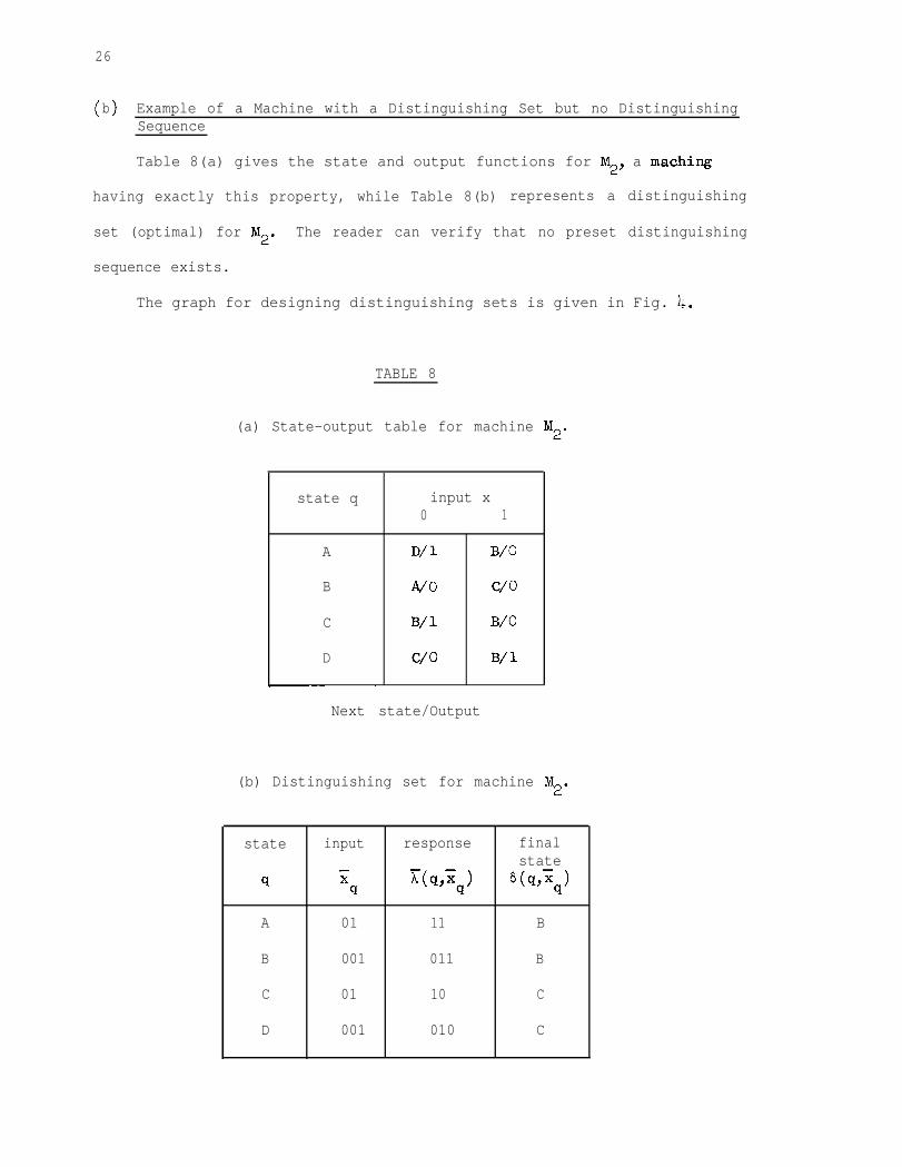
( >b Example of a Machine with a Distinguishing Set but no DistinguishingSequence
Table 8(a) gives the state and output functions for M2, a maching
having exactly this property, while Table 8(b) represents a distinguishing
set (optimal) for M2. The reader can verify that no preset distinguishing
sequence exists.
The graph for designing distinguishing sets is given in Fig. 4.
TABLE 8
(a) State-output table for machine M2.
state q input x0 1
A D/l B/O
B 4/O c/o
C B/l B/O
D c/o B/l_-~ _
Next state/Output
(b) Distinguishing set for machine Mz.
state input response finalstate
cl ";;q wb~q) 6 (Gq)
A 01 11 B
B 001 011 B
C 01 10 C
D 001 010 C

Fj \2, n
- 10 -
m-
c7
L- \0 7/
kL\
>

28
Design of a Checking Sequence Using 9
Initialization: synchronizing sequence 1001, leads to state B.
Checking part: the checking sequence is given in Table 9.
Again we use arrows to indicate where transitions are checked for the
first time. Other transitions are implicitly checked (e.g. 6(A,Ol) = B and
abo) = D checks 6(D,l) etc.). The length of this checking sequence is 31.
TABLE 9
Checking experiment for M2 using a distinguishing set.
0 0 1 0 0 1 0 0 0 0 1 0 1 0 0 0 1 (input)
B-A B A B A-D-C C C?-+B B (state)
0 1 1 0 1 1 0 1 0 1 0 1 0 1 0 1 1 (output)
(1) (3) (2) 4) (6)
..o 1 0
. . B A-+B
. . 0 1 0
(7)
(5)
c111001 (input)
B c-1B (state)
1 1 0 0 0 1 1 (output)
(8)
With locating sequences, the checking experiment becomes much longer.
Table 10 gives the sequences needed for the design. The synchronizing
sequence and the appearance of each locating sequence already require 35
symbols. All transition verifications still have to be performed.

29
TABLE 10
Construction of locating sequences for M2
characterizing setI
state input 1 input 01 locating, sequence
final finalresponse state response state
,
A 0 B 11 B (1o>4o1
B 0 C 00 B (1o)4o1
C 0 B 10 C (1U401
D 1 B 00 B 1

30
CONCLUSION
We have shown that checking experiments can be made considerably
shorter by using distinguishing sets. This is a consequence not only of
the shorter length of the sequences used for state identification but also
of the increased possibility for "telescoping" sequences and implicit
transition verification, as shown in the examples.
Further, in case no preset distinguishing sequence exists, a
distinguishing set, if one exists, can be used to replace the rather
cumbersome locating sequences.
As pointed out during the discussion of distinguishing sets, some
even more general approach might be possible. Indeed, if better use could
be made of all information given by a checking experiment, we might be able
to waive the restriction that the next input be the same for all elements
of a block (in the design graph). However, this would require a different
design philosophy. It is hoped that other simple methods will be found to
further reduce the length of checking experiments.

31
REFERENCES
[l] E. F. Moore, "Gedanken Experiments on Sequential Machines", Automata
Studies No. 34, pp. 129-153, Princeton University Press, Princeton,
NJ. (1956).
[2] F. C. Hennie, "Fault Detecting Experiments for Sequential Circuits",
Proc. 5th Ann. Symposium on Switching Theory and Logic Design, pp. 95-
110, Princeton, N.J. (Nov. 1964).
[3] F. C. Hennie, Finite State Models for Logical Machines, Wiley, New York
(1968).
L41 E. P. Hsieh, Optimal Checking Experiments for Sequential Machines,
Ph.D. dissertation, Columbia University, N.Y. (September 1969).
c51 E. P. Hsieh, "Checking experiments for Sequential Machines," IEEE
Transactions on Computers, Vol. C-20, No. 10, pp. 1153-1166 (October
1971).
[6] 3. Hartmanis, R. E. Stearns, Algebraic Structure Theory of Sequential
Machines, Prentice-Hall (1966).
[7] I. Kohavi, Z. Kohavi, "Variable-Length Distinguishing Sequences and
their application to Fault-Detection Experiments," IEEE Transactions
on Computers, vol. C-17, No. 8, pp. 792-795 (August 1968).

![[Y1997] Bit-Sequences an Adaptive Cache Invalidation Method in Mobile Client Server Environments](https://static.fdocuments.us/doc/165x107/577cd4771a28ab9e789897be/y1997-bit-sequences-an-adaptive-cache-invalidation-method-in-mobile-client.jpg)