Hierarchical structure and the prediction of missinglinks in networks

Aaron Clauset,1,3 Cristopher Moore,1,2,3 M. E. J. Newman3,4∗

1Department of Computer Science and2Department of Physics and Astronomy,

University of New Mexico, Albuquerque, NM 87131, USA3Santa Fe Institute, 1399 Hyde Park Rd., Santa Fe, NM 87501, USA

4Department of Physics and Center for the Study of Complex Systems,

University of Michigan, Ann Arbor, MI 48109, USA

∗To whom correspondence should be addressed. E-mail: mejn@umich.edu.

Networks have in recent years emerged as an invaluable tool for describing and quan-

tifying complex systems in many branches of science (1–3). Recent studies suggest that

networks often exhibit hierarchical organization, where vertices divide into groups that

further subdivide into groups of groups, and so forth over multiple scales. In many cases

these groups are found to correspond to known functional units, such as ecological niches

in food webs, modules in biochemical networks (protein interaction networks, metabolic

networks, or genetic regulatory networks), or communitiesin social networks (4–7). Here

we present a general technique for inferring hierarchical structure from network data

and demonstrate that the existence of hierarchy can simultaneously explain and quanti-

tatively reproduce many commonly observed topological properties of networks, such as

right-skewed degree distributions, high clustering coefficients, and short path lengths. We

further show that knowledge of hierarchical structure can be used to predict missing con-

nections in partially known networks with high accuracy, and for more general network

1

structures than competing techniques (8). Taken together, our results suggest that hierar-

chy is a central organizing principle of complex networks, capable of offering insight into

many network phenomena.

A great deal of recent work has been devoted to the study of clustering and community struc-

ture in networks (5,6,9–11). Hierarchical structure goes beyond simple clustering, however, by

explicitly including organization at all scales in a network simultaneously. Conventionally, hi-

erarchical structure is represented by a tree ordendrogramin which closely related pairs of

vertices have lowest common ancestors that are lower in the tree than those of more distantly

related pairs—see Fig. 1. We expect the probability of a connection between two vertices to

depend on their degree of relatedness. Structure of this type can be modeled mathematically us-

ing a probabilistic approach in which we endow each internalnoder of the dendrogram with a

probabilitypr and then connect each pair of vertices for whomr is the lowest common ancestor

independently with probabilitypr (Fig. 1c).

This model, which we call ahierarchical random graph, is similar in spirit (although differ-

ent in realization) to the tree-based models used in some studies of network search and naviga-

tion (12,13). Like most work on community structure, it assumes that communities at each level

of organization are disjoint. Overlapping communities have occasionally been studied (see, for

example, (14)) and could be represented using a more elaborate probabilistic model, but as we

discuss below the present model already captures many of thestructural features of interest.

Given a dendrogram and a set of probabilitiespr, the hierarchical random graph model

allows us to generate artificial networks with a specified hierarchical structure, a procedure

that might be useful in certain situations. Our goal here, however, is a different one. We

would like to detect and analyze the hierarchical structure, if any, of networks in the real world.

We accomplish this by fitting the hierarchical model to observed network data using the tools

of statistical inference, combining a maximum likelihood approach (15) with a Monte Carlo

2

sampling algorithm (16) on the space of all possible dendrograms. This technique allows us

to sample hierarchical random graphs with probability proportional to the likelihood that they

generate the observed network. To obtain the results described below we combine information

from a large number of such samples, each of which is a reasonably likely model of the data.

The success of this approach relies on the flexible nature of our hierarchical model, which

allows us to fit a wide range of network structures. The traditional picture of communities or

modules in a network, for example, corresponds to connections that are dense within groups of

vertices and sparse between them—a behavior called “assortativity” in the literature (17). The

hierarchical random graph can capture behavior of this kindusing probabilitiespr that decrease

as we move higher up the tree. Conversely, probabilities thatincrease up the tree correspond

to “disassortative” structures in which vertices are less likely to be connected on small scales

than on large ones. By letting thepr values vary arbitrarily throughout the dendrogram, the

hierarchical random graph can capture both assortative anddisassortative structure, as well as

arbitrary mixtures of the two, at all scales and in all parts of the network.

To demonstrate our method we have used it to construct hierarchical decompositions of

three example networks drawn from disparate fields: the metabolic network of the spirochete

Treponema pallidum(18), a network of associations between terrorists (19), and a food web of

grassland species (20). To test whether these decompositions accurately capturethe networks’

important structural features, we use the sampled dendrograms to generate new networks, dif-

ferent in detail from the originals but, by definition, having similar hierarchical structure (see the

Supplementary Information for more details). We find that these “resampled” networks match

the statistical properties of the originals quite closely,including degree distribution, clustering

coefficient, and distribution of shortest path lengths between pairs of vertices, despite the fact

that none of these properties is explicitly represented in the hierarchical random graph (Table 1

and Fig. 2a,b). Thus it appears that a network’s hierarchical structure is capable of explaining a

3

Network 〈k〉real 〈k〉samp Creal Csamp dreal dsamp

T. pallidum 4.8 3.7(1) 0.0625 0.0444(2) 3.690 3.940(6)Terrorists 4.9 5.1(2) 0.361 0.352(1) 2.575 2.794(7)Grassland 3.0 2.9(1) 0.174 0.168(1) 3.29 3.69(2)

Table 1: Comparison of network statistics for the three example networks studied and newnetworks generated by resampling from our hierarchical model. The generated networks closelymatch the average degree〈k〉, clustering coefficientC, and average vertex-vertex distanced ineach case, suggesting that they capture much of the real networks’ structure. Parentheticalvalues indicate standard errors on the final digits.

wide variety of other network features as well.

The dendrograms produced by our method are also of interest in themselves, as a graphical

representation and summary of the hierarchical structure of the observed network. As discussed

above, our method typically generates not just a single dendrogram but a set of dendrograms,

each of which is a good fit to the data. From this set we can, using techniques from phylogeny

reconstruction (21), create a singleconsensus dendrogram, which captures the topological fea-

tures that appear consistently across all or a large fraction of the dendrograms and typically rep-

resents a better summary of the network’s structure than anyindividual dendrogram. Figure 2c

shows such a consensus dendrogram for the grassland speciesnetwork, which clearly reveals

communities and sub-communities of plants, herbivores, parasitoids, and hyper-parasitoids.

Another application of the hierarchical decomposition is in the prediction of missing in-

teractions in networks. In many settings, the discovery of interactions in a network requires

significant experimental effort in the laboratory or the field. As a result, our current pictures

of many networks are substantially incomplete (22–29). An attractive alternative to checking

exhaustively for a connection between every pair of vertices in a network is to try to predict,

in advance and based on the connections already observed, which vertices are most likely to

be connected, so that scarce experimental resources can be focused on testing for those interac-

tions. If our predictions are good, we can in this way reduce substantially the effort required to

4

establish the network’s topology.

The hierarchical decomposition can be used as the basis for an effective method of predict-

ing missing interactions as follows. Given an observed but incomplete network, we generate as

described above a set of hierarchical random graphs—dendrograms and the associated proba-

bilities pr—that fit that network. Then we look for pairs of vertices thathave a high average

probability of connection within these hierarchical random graphs but which are unconnected

in the observed network. These pairs we consider the most likely candidates for missing con-

nections. (Technical details of the procedure are given in the Supplementary Information.)

We demonstrate the method using our three example networks again. For each network we

remove a subset of connections chosen uniformly at random and then attempt to predict, based

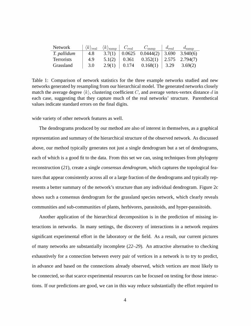
on the remaining connections, which ones have been removed.A standard metric for quantify-

ing the accuracy of prediction algorithms, commonly used inthe medical sciences and machine

learning communities, is the AUC statistic, which is equivalent to the area under the receiver-

operating characteristic (ROC) curve (see, for example, (30)). In the present context, the AUC

statistic can be interpreted as the probability that a randomly chosen missing connection (a true

positive) is given a higher score by our method than a randomly chosen pair of unconnected

vertices (a true negative). Thus, the degree to which the AUCexceeds0.5 indicates how much

better our predictions are than chance. Figure 3 shows the AUC statistic for the three networks

as a function of the fraction of the connections known to the algorithm. For all three networks

our algorithm does far better than chance, indicating that hierarchy is a strong general predictor

of missing structure.

It is also instructive to compare the performance of our method to that of other methods for

link prediction (8). Previously proposed methods include assuming that vertices are likely to be

connected if they have many common neighbors, if there are short paths between them, or if the

product of their degrees is large. These approaches work well for strongly assortative networks

5

such as the collaboration and citation networks studied in (8) and for the metabolic and terrorist

networks studied here (Fig. 3a,b). Indeed, for the metabolic network, the shortest-path heuristic

performs better than our algorithm.

However, these simple methods can be misleading for networks that exhibit more general

types of structure. In food webs, for instance, pairs of predators often share prey species, but

rarely prey on each other. In such situations a common-neighbor or shortest-path-based method

would predict connections between predators where none exist. The hierarchical model, by

contrast, is capable of expressing both assortative and disassortative structure and, as Fig. 3c

shows, gives substantially better predictions for the grassland network. (Indeed, in Fig. 2d there

are several groups of parasitoids that our algorithm has grouped together in a disassortative

community, in which they prey on the same herbivore but not oneach other.) The hierarchi-

cal method thus makes accurate predictions for a wider rangeof network structures than the

alternative methods above.

In the applications above, we have assumed for simplicity that there are no false positives

in our network data, i.e., that every observed edge corresponds to a real interaction. In net-

works where false positives may be present, however, they too could be predicted using the

same approach: we would simply look for pairs of vertices that have alow average probability

of connection within the hierarchical random graph but which are connected in the observed

network.

The method described here could also be extended to incorporate domain-specific informa-

tion, such as morphological or behavioral traits in food webs (29) or phylogenetic or binding-

domain data for biochemical networks (23), by adjusting the probabilities of edges accordingly.

As the results above show, however, we can obtain good predictions even in the absence of such

information, indicating that topology alone can provide rich insights.

In closing, we note that our approach differs crucially fromprevious work on hierarchical

6

structure in networks (1, 4–7, 9, 11, 31) in that it acknowledges explicitly that most real-world

networks have many plausible hierarchical representations of roughly equal likelihood. Pre-

vious work, by contrast, has typically sought a single hierarchical representation for a given

network. By sampling an ensemble of dendrograms, our approach avoids over-fitting the data

and allows us to explain many common topological features, generate resampled networks with

similar structure to the original, derive a clear and concise summary of a network’s structure

via its consensus dendrogram, and accurately predict missing connections in a wide variety of

situations.

Acknowledgments: The authors thank Chris Wiggins, Cosma Shalizi, Jennifer Dunne, Michael

Gastner, Mason Porter, Petter Holme, and Mikael Huss for their help. CM thanks the Center for

the Study of Complex Systems at the University of Michigan fortheir hospitality while some of

this work was conducted. This work was supported by the National Science Foundation under

grants PHY–0200909 (AC, CM), ITR–0324845 (AC, CM) and DMS–0405348 (MEJN), by a

grant from the James S. McDonnell Foundation (MEJN), and by the Santa Fe Institute (AC,

CM, MEJN).

References

1. S. Wasserman, K. Faust,Social Network Analysis(Cambridge University Press, Cam-

bridge, 1994).

2. R. Albert, A.-L. Barabasi,Rev. Mod. Phys.74, 47 (2002).

3. M. E. J. Newman,SIAM Review45, 167 (2003).

4. E. Ravasz, A. L. Somera, D. A. Mongru, Z. N. Oltvai, A.-L. Barabasi, Science30, 1551

(2002).

7

5. A. Clauset, M. E. J. Newman, C. Moore,Phys. Rev. E70, 066111 (2004).

6. R. Guimera, L. A. N. Amaral,Nature433, 895 (2005).

7. M. C. Lagomarsino, P. Jona, B. Bassetti, H. Isambert,Proc. Natl. Acad. Sci. USA104, 5516

(2001).

8. D. Liben-Nowell, J. Kleinberg,International Conference on Information and Knowledge

Management(2003). It should be noted that this paper focuses on predicting future con-

nections given current ones, as opposed to predicting connections which exist but have not

yet been observed.

9. M. Girvan, M. E. J. Newman,Proc. Natl. Acad. Sci. USA99, 7821 (2002).

10. A. E. Krause, K. A. Frank, D. M. Mason, R. E. Ulanowicz, W. W.Taylor,Nature426, 282

(2003).

11. F. Radicchi, C. Castellano, F. Cecconi, V. Loreto, D. Parisi,Proc. Natl. Acad. Sci. USA101,

2658 (2004).

12. D. J. Watts, P. S. Dodds, M. E. J. Newman,Science296, 1302 (2002).

13. J. M. Kleinberg,Proceedings of the 2001 Neural Information Processing Systems Confer-

ence, T. G. Dietterich, S. Becker, Z. Ghahramani, eds. (MIT Press,Cambridge, MA, 2002).

14. G. Palla, I. Derenyi, I. Farkas, T. Vicsek,Nature435, 814 (2005).

15. G. Casella, R. L. Berger,Statistical Inference(Duxbury Press, Belmont, 2001).

16. M. E. J. Newman, G. T. Barkema,Monte Carlo Methods in Statistical Physics(Clarendon

Press, Oxford, 1999).

8

17. M. E. J. Newman,Phys. Rev. Lett.89, 208701 (2002).

18. M. Huss, P. Holme, Currency and commodity metabolites: Their identification and relation

to the modularity of metabolic networks. (2006). Preprintq-bio.MN/0603038.

19. V. Krebs,Connections24, 43 (2002).

20. H. A. Dawah, B. A. Hawkins, M. F. Claridge,Journal of Animal Ecology64, 708 (1995).

21. D. Bryant, BioConsensus, M. Janowitz, F.-J. Lapointe, F. R. McMorris, B. Mirkin,

F. Roberts, eds. (DIMACS, 2003), pp. 163–184.

22. J. A. Dunne, R. J. Williams, N. D. Martinez,Proc. Natl. Acad. Sci. USA99, 12917 (2002).

23. A. Szilagyi, V. Grimm, A. K. Arakaki, J. Skolnick,Physical Biology2, S1 (2005).

24. E. Sprinzak, S. Sattath, H. Margalit,J. Mol. Biol.327, 919 (2003).

25. T. Ito,et al., Proc. Natl. Acad. Sci. USA98, 4569 (2001).

26. A. Lakhina, J. W. Byers, M. Crovella, P. Xie,Proc. INFOCOM(2003).

27. A. Clauset, C. Moore,Phys. Rev. Lett.94, 018701 (2005).

28. D. Achlioptas, A. Clauset, D. Kempe, C. Moore,Proc. Symposium on Theory of Computing

(STOC)(2005), pp. 694–703.

29. N. D. Martinez, B. A. Hawkins, H. A. Dawah, B. P. Feifarek,Ecology80, 1044 (1999).

30. J. A. Hanely, B. J. McNeil,Radiology143, 29 (1982).

31. M. Sales-Pardo, R. Guimera, A. A. Moreira, L. A. N. Amaral, Extracting and representing

the hierarchical organization of complex systems (2006). Unpublished manuscript.

9

Supplementary Information

A Hierarchical Random Graphs

Our model for the hierarchical organization of a network is as follows. LetG be a graph withn

vertices. AdendrogramD is a binary tree withn leaves corresponding to the vertices ofG. Each

of then − 1 internal nodes ofD corresponds to a group of vertices that are descended from it.

We associate a probabilitypr with each internal noder. Then, given two verticesi, j of G, the

probabilitypij that they are connected by an edge ispij = pr wherer is their lowest common

ancestor inD. The combination(D, {pr}) of the dendrogram and the set of probabilities then

defines ahierarchical random graph.

Note that if a community has, say, three subcommunities, with an equal probabilityp of

connections between them, we can represent this in our modelby first splitting one of these

subcommunities off, and then splitting the other two. The two internal nodes corresponding to

these splits would be given the same probabilitiespr = p. This yields three possible binary

dendrograms, which are all considered equally likely.

We can think of the hierarchical random graph as a variation on the classical Erdos–Renyi

random graphG(n, p). As in that model, the presence or absence of an edge between any pair

of vertices is independent of the presence or absence of any other edge. However, whereas

in G(n, p) every pair of vertices has the same probabilityp of being connected, in the hierar-

chical random graph the probabilities are inhomogeneous, with the inhomogeneities controlled

by the topological structure of the dendrogramD and the parameters{pr}. Many other models

with inhomogeneous edge probabilities have, of course, been studied in the past. Examples

include the widely-studied configuration model1 and structured random graphs in which there

are a finite number of types of vertices with a matrixpkl giving the connection probabilities

1M. Molloy and B. Reed, “A critical point for random graphs with a given degree sequence”,Random Structuresand Algorithms6, 161–179 (1995)

10

between them.2

B Fitting the hierarchical random graph to data

Now we turn to the question of finding the hierarchical randomgraph or graphs that best fits

the observed real-world networkG. Assuming that all hierarchical random graphs area priori

equally likely, the probability that a given model(D, {pr}) is the correct explanation of the

data is, by Bayes’ theorem, proportional to the posterior probability or likelihoodL with which

that model generates the observed network.3 Our goal is to maximizeL or, more generally, to

sample with probability proportional toL from the space of all models.

Let Er be the number of edges inG whose endpoints haver as their lowest common an-

cestor inD, and letLr andRr, respectively, be the numbers of leaves in the left and right

subtrees rooted atr. Then the likelihood of the hierarchical random graph (consisting of the

dendrogramD and the set of probabilities{pr}) is

L(D, {pr}) =∏

r∈D

pEr

r (1 − pr)LrRr−Er (1)

with the convention that00 = 1.

If we fix the dendrogramD, it is easy to find the probabilities{pr} that maximizeL(D, {pr}).

For eachr, they are given by

pr =Er

LrRr

, (2)

the fraction of potential edges between the two subtrees ofr that actually appear in the graphG.

The likelihood of the dendrogram evaluated at the maximum isthen

L(D) =∏

r∈D

[

p pr

r (1 − pr)1−p

r

]LrRr

. (3)

2F. McSherry, “Spectral Partitioning of Random Graphs,”Proc. Foundations of Computer Science (FOCS), pp.529–537 (2001)

3G. Casella and R. L. Berger, “Statistical Inference.” Duxbury Press, Belmont (2001).

11

Figure 4 shows an illustrative example, consisting of a network with six vertices.

It is often convenient to work with the logarithm of the likelihood,

logL(D) = −∑

r∈D

LrRrh(pr), (4)

whereh(p) = −p log p − (1 − p) log(1 − p) is the Gibbs-Shannon entropy function. Note that

each term−LrRrh(pr) is maximized whenpr is close to0 or to 1, i.e., when the entropy is

minimized. In other words, high-likelihood dendrograms are those that partition the vertices

into groups between which connections are either very common or very rare.

We now use a Markov chain Monte Carlo method to sample dendrogramsD with probability

proportional to their likelihoodL(D). To create the Markov chain we need to pick a set of

transitions between possible dendrograms. The transitions we use consist of rearrangements of

subtrees of the dendrogram as follows. First, note that eachinternal noder of a dendrogramD

is associated with three subtrees: the subtreess, t descended from its two daughters, and the

subtreeu descended from its sibling. As Figure 5 shows, there are two ways we can reorder

these subtrees without disturbing any of their internal relationships. Each step of our Markov

chain consists first of choosing an internal noder uniformly at random (other than the root) and

then choosing uniformly at random between the two alternateconfigurations of the subtrees

associated with that node and adopting that configuration. The result is a new dendrogramD′.

It is straightforward to show that transitions of this type are ergodic, i.e., that any pair of finite

dendrograms can be connected by a finite series of such transitions.

Once we have generated our new dendrogramD′ we accept or reject that dendrogram

according to the standard Metropolis–Hastings rule (16). Specifically, we accept the transi-

tion D → D′ if ∆ logL = logL(D′) − logL(D) is nonnegative, so thatD′ is at least as likely

asD; otherwise we accept the transition with probabilityexp(log ∆L) = L(D′)/L(D). If the

transition is not accepted we revert to the original dendrogramD again on this step of the chain.

12

The Metropolis-Hastings rule ensures detailed balance and, in combination with the ergodic

transition set, guarantees a limiting probability distribution over dendrograms that is propor-

tional to the likelihood,P (D) ∝ L(D). The quantity∆ logL can be calculated easily, since

the only terms in Eq. (4) that change fromD to D′ are those involving the subtreess, t, andu

associated with the chosen node.

The Markov chain appears to converge relatively quickly, with the likelihood reaching a

plateau after roughlyO(n2) steps. This is not a rigorous performance guarantee, however, and

indeed there are mathematical results for similar Markov chains that suggest that equilibration

could take exponential time in the worst case.4 Still, as our results here show, the method seems

to work quite well in practice. The algorithm is able to handle networks with up to a few

thousand vertices in a reasonable amount of computer time.

We find that there are typically many dendrograms with roughly competitive likelihoods,

which reinforces our contention that it is important to sample the distribution of dendrograms

rather than merely focusing on the most likely one.

C Resampling from the hierarchical random graph

The procedure for resampling from the hierarchical random graph is as follows.

1. Initialize the Markov chain by choosing a random startingdendrogram.

2. Run the Monte Carlo algorithm until equilibrium is reached.

3. Sample dendrograms at regular intervals thereafter fromthose generated by the Markov

chain.4E. Mossel and E. Vigoda, “Phylogenetic MCMC Are Misleading on Mixtures of Trees.”Science309, 2207

(2005)

13

4. For each sampled dendrogramD, create a resampled graphG′ with n vertices by placing

an edge between each of then(n − 1)/2 vertex pairs(i, j) with independent probabil-

ity pr, wherer is the lowest common ancestor ofi andj in D andpr is given by Eq. (2).

(In principle, there is nothing to stop us generating many resampled graphs from a den-

drogram, but in the calculations described in this paper we generate only one from each

dendrogram.)

After generating many samples in this way, we can compute averages of network statistics such

as the degree distribution, the clustering coefficient, thevertex-vertex distance distribution, and

so forth. Thus, in a way similar to Bayesian model averaging,5 we can estimate the distribution

of network statistics defined by the equilibrium ensemble ofdendrograms.

For the construction of consensus dendrograms such as the one shown in Fig. 2c, we found

it useful to weight the most likely dendrograms more heavily, giving them weight proportional

to the square of their likelihood, in order to extract a coherent consensus structure from the

equilibrium set of models.

D Predicting Missing Connections

Our algorithm for using hierarchical random graphs to predict missing connections is as follows.

1. Initialize the Markov chain by choosing a random startingdendrogram.

2. Run the Monte Carlo algorithm until equilibrium is reached.

3. Sample dendrograms at regular intervals thereafter fromthose generated by the Markov

chain.5T. Hastie, R. Tibshirani and J. Friedman, “The Elements of Statistical Learning.” Springer, New York (2001).

14

4. For each pair of verticesi, j for which there is not already a known connection, calculate

the mean probability〈pij〉 that they are connected by averaging over the corresponding

probabilitiespij in each of the sampled dendrogramsD.

5. Sort these pairsi, j in decreasing order of〈pij〉 and predict that the highest ranked ones

have missing connections.

In general, we find that the top 1% of such predictions are highly accurate. However, for

large networks, even the top 1% can be an unreasonably large number of candidates to check

experimentally. In many contexts, researchers may want to consider using the procedure inter-

actively, i.e., predicting a small number of missing connections, checking them experimentally,

adding the results to the network, and running the algorithmagain to predict additional connec-

tions.

The alternative prediction methods we compared against, which were previously investi-

gated in (8), consist of giving each pairi, j of vertices a score, sorting pairs in decreasing order

of their score, and predicting that those with the highest scores are the most likely to be con-

nected. Several different types of scores were investigated, defined as follows, whereΓ(j) is

the set of vertices connected toj.

1. Common neighbors: score(i, j) = |Γ(i) ∩ Γ(j)|, the number of common neighbors of

verticesi andj.

2. Jaccard coefficient: score(i, j) = |Γ(i) ∩ Γ(j)| / |Γ(i) ∪ Γ(j)|, the fraction of all neigh-

bors ofi andj that are common neighbors of both.

3. Degree product: score(i, j) = |Γ(i)| |Γ(j)|, the product of the degrees ofi andj.

4. Short paths: score(i, j) is 1 divided by the length of the shortest path through the network

from i to j (or zero for vertex pairs that are not connected by any path).

15

One way to quantify the success of a prediction method, used by previous authors who have

studied link prediction problems (8), is the ratio between the probability that the top-ranked pair

is connected and the probability that a randomly chosen pairof vertices, which do not have an

observed connection between them, are connected. Figure 6 shows the average value of this

ratio as a function of the percentage of the network shown to the algorithm, for each of our

three networks. Even when fully50% of the network is missing, our method predicts missing

connections about ten times better than chance for all threenetworks. In practical terms, this

means that the amount of work required of the experimenter todiscover a new connection is

reduced by a factor of10, an enormous improvement by any standard. If a greater fraction of

the network is known, the accuracy becomes even greater, rising as high as200 times better

than chance when only a few connections are missing.

We note, however, that this using this ratio to judge prediction algorithms has an important

disadvantage. Some missing connections are much easier to predict than others: for instance, if

a network has a heavy-tailed degree distribution and we remove a randomly chosen subset of the

edges, the chances are excellent that two high-degree vertices will have a missing connection

and such a connection can be easily predicted by simple heuristics such as those discussed

above. The AUC statistic used in the text, by contrast, looksat an algorithm’s overall ability to

rank all the missing connections over nonexistent ones, notjust those that are easiest to predict.

Finally, we have investigated the performance of each of theprediction algorithms on purely

random (i.e., Erdos–Renyi) graphs. As expected, no method performs better than chance in this

case, since the connections are completely independent random events and there is no structure

to discover. We also tested each algorithm on a graph with a power-law degree distribution

generated according to the configuration model. In this case, guessing that high-degree vertices

are likely to be connected performs quite well, whereas the method based on the hierarchical

random graph performs poorly since these graphs have no hierarchical structure to discover.

16

a b c

Figure 1:a, A simple network with no hierarchical structure and the corresponding dendrogram.b, A network with a single level of community structure and itsdendrogram.c, A hierarchicalnetwork with structure on many scales and the correspondinghierarchical random graph. In thehierarchical random graph the dendrogram structure is augmented by defining for each internalnoder a probabilitypr that a pair of vertices in the left and right subtrees of that node areconnected. (The shades of the internal nodes in the figure represent the probabilities.)

17

100

101

10−3

10−2

10−1

100a

Degree, k

Fra

ctio

n of

ver

tices

with

deg

ree

k

2 4 6 8 1010

−3

10−2

10−1

100b

Distance, dF

ract

ion

of v

erte

x−pa

irs a

t dis

tanc

e d

c d

Figure 2: Application of our hierarchical decomposition tothe network of grassland speciesinteractions.a, Original (blue) and resampled (red) degree distributions. b, Original and resam-pled distributions of vertex-vertex distances.c, Consensus dendrogram reconstructed from thesampled hierarchical models.d, A visualization of the network in which the upper few levelsof the consensus dendrogram are shown as boxes around species (plants©, herbivores�, par-asitoids▽, hyper-parasitoids△ and hyper-hyper-parasitoids⋄). Note that in several cases, aset of parasitoids is grouped into a community by our algorithm, not because they prey on eachother, but because they prey on the same herbivore.

18

0 0.2 0.4 0.6 0.8 10.4

0.5

0.6

0.7

0.8

0.9

1

AU

C

Fraction of edges observed

Terrorist association networka

Pure chanceCommon neighborsJaccard coefficientDegree productShortest pathsHierarchical structure

0 0.2 0.4 0.6 0.8 10.4

0.5

0.6

0.7

0.8

0.9

1

AU

C

Fraction of edges observed

T. pallidum metabolic networkb

Pure chanceCommon neighborsJaccard coefficientDegree productShortest pathsHierarchical structure

0 0.2 0.4 0.6 0.8 10.4

0.5

0.6

0.7

0.8

0.9

1

AU

C

Fraction of edges observed

Grassland species networkc

Pure chanceCommon neighborsJaccard coefficientDegree productShortest pathsHierarchical structure

Figure 3: Comparison of link prediction methods. Average area under the curve (AUC) statisticfor the receiver-operating characteristic (ROC), as a function of the fraction of connectionsknown to the algorithm, for the link prediction method presented here and a variety of previouslypublished methods.

19

a

b

c d

e

f

a b c d e f

1

1

1

1

1/9

a b c d e f

1

1

1

1/3

1/4

Figure 4: An example networkG consisting of six vertices, and the likelihood of two possi-ble dendrograms. The internal nodesr of each dendrogram are labeled with the maximum-likelihood probability pr, i.e., the fraction of potential edges between their left and rightsubtrees that exist inG. According to Eq. (3), the likelihoods of the two dendrogramsareL(D1) = (1/3)(2/3)2 ·(1/4)2(3/4)6 = 0.00165 . . . andL(D2) = (1/9)(8/9)8 = 0.0433 . . .The second dendrogram is far more likely because it correctly divides the network into twohighly-connected subgraphs at the first level.

i

s t u uts s u t

Figure 5: Each internal noder of the dendrogram has three associated subtreess, t, andu,which can be placed in any of three configurations. (Note thatthe topology of the dendrogramdepends only on the sibling and parent relationships; the order, left to right, in which they aredepicted is irrelevant).

20

0 0.1 0.2 0.3 0.4 0.5 0.6 0.7 0.8 0.9 11

2

10

20

100

200

Fraction of edges observed

Fac

tor

of im

prov

emen

t ove

r ch

ance

Terrorist association networka

Common neighborsJaccard coefficientDegree productShortest pathsHierarchical structure

0 0.1 0.2 0.3 0.4 0.5 0.6 0.7 0.8 0.9 11

2

10

20

100

200

Fraction of edges observed

Fac

tor

of im

prov

emen

t ove

r ch

ance

T. pallidum metabolic networkb

Common neighborsJaccard coefficientDegree productShortest pathsHierarchical structure

0 0.1 0.2 0.3 0.4 0.5 0.6 0.7 0.8 0.9 11

2

10

20

100

200

Fraction of edges observed

Fac

tor

of im

prov

emen

t ove

r ch

ance

Grassland species networkc

Common neighborsJaccard coefficientDegree productShortest pathsHierarchical structure

Figure 6: Further comparison of link prediction algorithms. Data points represent the averageratio between the probability that the top-ranked pair of vertices is in fact connected and thecorresponding probability for a randomly-chosen pair, as afunction of the fraction of the con-nections known to the algorithm. For each network (a, Terrorist associations;b, T. pallidummetabolites; andc, Grassland species interactions), we compare our method with simpler meth-ods such as guessing that two vertices are connected if they share common neighbors, have ahigh degree product, or have a short path between them.

21