Hands on Shape from Shading - Scientific …gerig/CS6320-S2015/Materials/Elhabian...To do this,...

Shireen Elhabian Spring 2008

1

Hands on Shape from Shading

Technical Report

May 2008

by

Shireen Y. Elhabian

Computer Vision and Image Processing (CVIP) Laboratory

Electrical and Computer Engineering Department

University of Louisville

Louisville, KY 40292

Table of Contents

1. Basic Idea ................................................................................................................................................ 2

2. Terminology ............................................................................................................................................ 3 2.1 Surface normal .................................................................................................................................. 3 2.2 Illumination direction........................................................................................................................ 4

2.3 Surface types ..................................................................................................................................... 5 2.4 The viewer (camera) ......................................................................................................................... 6

3. The simplest scenario .............................................................................................................................. 6 4. Synthetic image generation ..................................................................................................................... 7

4.1 Lets do it … ...................................................................................................................................... 7 5. Problem statement ................................................................................................................................. 10

6. Finding surface albedo and illumination direction ............................................................................... 11 6.1 Assumptions .................................................................................................................................... 11 6.2 Simple method for Lambertian surfaces ......................................................................................... 12

7. Shape from shading as a minimization problem ................................................................................... 16 7.1 The functional to be minimized ...................................................................................................... 17 7.2 The Euler-Lagrange equations ........................................................................................................ 18

7.3 From the continuous to the discrete case ........................................................................................ 19 7.4 The algorithm .................................................................................................................................. 19 7.5 Enforcing integrability .................................................................................................................... 20

7.6 Let’s do it ........................................................................................................................................ 21 8. Linear approaches ................................................................................................................................. 28

8.1 Pentland [6] approach ..................................................................................................................... 28 Let’s do it … ................................................................................................................................. 29

8.2 Shah [7] approach ........................................................................................................................... 32 Let’s do it … ................................................................................................................................. 33

Now ........................................................................................................................................................... 37 References ................................................................................................................................................. 37


2

1. Basic Idea

Figure 1 – Shape from shading problem [5]

Given an input gray-scale image, we want to recover the 3D information of the captured (imaged)

object. The observed (measured/captured) intensity of an image depends on four main factors:

Illumination, which is defined by its position, direction and spectral energy distribution ( omni

directional, spot light …).

Surface reflectivity of the object, which is known in shape from shading literature as albedo, it

entails the information about how the object reacts with light in terms of the amount of incident

light being reflected, in computer graphics literature, it is denoted as surface reflectance

coefficients or more commonly as surface material.

Surface geometry of an object, which we want to recover given the object's 2D gray-scale

image.

Camera capturing the object, which is defined by its intrinsic and extrinsic parameters.

Computer graphics deals with simulating the image formation process, i.e. given the 3D surface

geometry, illumination direction and surface reflectivity, an image is rendered to simulate the camera

process. However, in principle, shape from shading is the inverse problem, given an image, a model of

the illumination and a model of the surface reflectivity; it is required to recover the surface geometry.


3

Yet inverse problems often are ill-posed, since we have more unknown parameters than equations (given

information). To solve such problems, we should impose appropriate assumptions.

If the surface normal is known at every point on the surface, surface geometry can be known up to scale;

hence most of the shape from shading algorithms are seeking the recovery of surface normals.

2. Terminology

Figure 2 - A 3D surface is illuminated by a light source defined by its direction, and captured by a camera (viewer)

defined by its direction where the surface normal is the unit vector perpendicular on the suface.

2.1 Surface normal

The orientation of a surface can be completely defined by defining the normal to the surface at every

point (x,y,z). Let n = (nx,ny,nz) be a unit vector giving the surface normal at point (x,y,z).

For the computations to follow, it is useful to define the normal by its spherical not Cartesian

coordinates, hence n can be defined by its tilt n and slant n, where the tilt (or azimuth angle) is define

as the angle between the x-axis and the projection of n on the xy-plane, and the slant (or polar angle) is

defined as the angle between the z-axis and the normal. Hence the surface normal is defined as n(n,n)

where n[0,/2] is the slant angle and n[0,2] is the tilt angle.

From the relation between the Cartesian and spherical coordinates, we can obtain the slant and tilt angles

from (xn,yn,zn) as follows;

x

y

nn

n1tan (1)


4

zn n1cos (2)

Hence the normal vector can be defined as:

T

nnnnnzyx nnnn ]cos,sinsin,cos[sin),,( (3)

Another representation of surface orientation is by its gradient, let the surface be given by Z = Z(x,y),

hence the gradient (p,q)T at point (x,y,Z(x,y)) is simply the partial derivative in x and y directions and can

be given by the surface slopes (1,0,p) and (0,1,q) where;

x

yxZp

),( (4)

y

yxZq

),( (5)

The relation between the surface gradient and the surface normal can be derived from the fact that

surface slopes (1,0,p) and (0,1,q) are two vectors lying on the tangent plane at point (x,y,z), hence the

surface normal can be obtained by the cross product of these vectors to result in a vector perpendicular

to the tangent plane, then normalizing it to be a unit vector, hence the normal vector can be expressed in

terms of surface gradients as a point (p,q) in the gradient space as follows;

Tqpqp

n ]1,,[1

122

(6)

2.2 Illumination direction

This is the direction from which the object is illuminated. Similar to the representation of the surface

normal, we can represent the illumination direction in terms of its slant and tilt as I(,) where

[0,/2] is the slant angle and [0,2] is the tilt angle. Hence the illumination direction can be

defined as follows;

TI ]cos,sinsin,cos[sin (7)


5

2.3 Surface types

In order to see an object, there should be a light source; emitting light, then the object will either absorb

the entire incident light or reflect all of it, or even reflect some and absorb the rest. This phenomena

defines the surface reflectivity, which is the fraction of incident light (radiation) reflected by a surface.

In general, surface reflectivity is a function of the reflected direction and the incident direction; hence it

is a directional property. Most of the surfaces can be divided into those that are specular and those that

are diffuse. For specular surfaces, such as glass or polished metal, reflectivity will be nearly zero at all

angles except at the appropriate reflected angle where the surface shines. For diffuse surfaces, such as

matte white paint, reflectivity is uniform, light is reflected in all angles equally or near-equally, such

surfaces are said to be Lambertian. Most real objects have some mixture of diffuse and specular

reflective properties.

For a Lambertian surface, the intensity only depends on the angle between the illumination direction

and the surface normal, hence under Lambertian assumption, the reflectance at point (x,y,z) is a function

of the angle and the surface reflectivity (albedo) defined as follows;

cos),,(),,( zyxzyxR (8)

In (8) the angle between the illumination direction and the surface normal is assumed to be fixed with

respect to the surface point (x,y,z) under the assumption that all visible surface points will receive the

same amount of light from the same direction, i.e. the illumination direction will not be changed from a

point to another on the same surface. However according to the surface of interest, the albedo might

change from one point to another, however there are some shape from shading algorithms which assume

constant albedo over the surface to facilitate problem solution, yet this is not a realistic assumption.

Using unit vectors for the illumination direction and the surface normal, (8) can be rewritten as follows;

for simplicity we will refer to ),,( zyx as simply since we are mainly interested in surface geometry

under the assumption of either given or estimate surface albedo.

TTT

I qpqp

qpR ]1,,[1

),(22,

InI

(9)


6

Eq(9) implies that given the surface albedo and the illumination direction, the reflectance map IR , at a

point (p,q) defined in the gradient space can be expressed in terms of the dot product of the surface

normal and the illumination direction, scaled by the surface albedo.

2.4 The viewer (camera)

A camera is a projective system; it projects 3D point to 2D image pixels. To model the camera process,

we use projections models such as perspective and orthographic projection. Under the assumption of

orthographic projection, a point (X,Y,Z) can be projected to a 2D point (x,y) such that x = mX and y =

mY, where m is a magnification factor of our choice. While using perspective projection, the 2D point

will be defined as x = X/Z and y = Y/Z.

3. The simplest scenario

We will be concerned with the simplest scenario, where the following assumptions hold;

Camera; orthographic projection.

Surface reflectivity; Lambertian surface

Known/estimated illumination direction.

Known/estimated surface albedo/

The optical axis is the Z axis of the camera and the surface can be parameterized as Z = Z(x,y).

The image irradiance (amount of light received by the camera to which the gray-scale produced is

directly proportional) can be defined as follows;

TTT

I qpqp

qpRyxE ]1,,[1

),(),(22,

InI

(10)

Eq(10) is the typical starting point of many shape from shading techniques, yet it is of a great

mathematical complexity, it is a non-linear partial differential equation in p = p(x,y) and q = q(x,y),

which are the gradients of the unknown surface Z = Z(x,y) and depends on quantities not necessarily

known (albedo, illumination direction and boundary conditions on which the partial differential equation

is dependent). In essence the solution is determined uniquely only if certain a priori information on the


7

solution is available. This information is typically given at the boundary of the domain of interest, in our

case, the image boundaries.

4. Synthetic image generation

The best way to grasp the meaning of (10) is to produce a synthetic shaded image ourselves. To do this,

first we assume Lambertian surface, we then write the equation of our favorite surface in the form of Z =

Z(x,y), choose value(s) for the surface albedo, specify illumination direction, then compute the

numerical partial derivatives of the surface Z over a pixel grid, then compute the corresponding image

brightness using (10).

4.1 Lets do it …

Lets generate the 2D image of a sphere, the equation of a sphere of center (0,0,0) and radius r can be

given as follows;

2222 rzyx (11)

Step 1:

Write the above equation in the form of Z = Z(x,y):

2222222 yxrzyxrz (12)

Since when a sphere is imaged, only a hemisphere appears in the captured image, and the other

hemisphere is not visible, hence we will take either the positive or the negative root. Hence our

surface equation can be written as follows;

222 yxrz (13)

% sphere radius ... r = 50;

% lets define the xy domain (pixel grid)... x and y are data grids % (matrices) where the our surface Z = Z(x,y) can be calculated at % each point (x,y).


8

% use finner grid to enhance the resolution [x,y] = meshgrid(-1.5*r:0.1:1.5*r,-1.5*r:0.1:1.5*r);

Step 2:

Assume constant albedo over the points of the sphere surface, let =0.5, this means that our

sphere will reflect 50% of the incident light.

% surface albedo ... albedo = 0.5;

Step 3:

Choose the illumination direction, let, I = [0.2, 0, 0.98]T .

% illumination direction ... I = [0.2 0 0.98]';

Step 4:

Derive the surface partial derivates as follows; in the x-direction

21

22221

222 22

1),(

yxrxxyxr

x

yxZp (14)

Likewise in the y-direction,

21

22221

222 22

1),(

yxryyyxr

y

yxZq (15)

% surface partial derivates at each point in the pixel grid ... p = -x./sqrt(r^2-(x.^2 + y.^2)); % in the x direction q = -y./sqrt(r^2-(x.^2 + y.^2)); % in the y direction

Step 5:

Compute the image brightness using (10), it can be rewritten as follows;


9

2222 1

]1,,][,,[1

),(qp

iqipiqpiii

qpyxE

zyxT

zyx

(16)

where I = ],,[ zyx iiiT

Note that for certain illuminants, some image locations might violate the assumption that all

visible surface points receive direct illumination, e.g. donut being illuminated from one side,

hence the image brightness computed from (10) become negative, in this case the brightness

should be set to zero.

% now lets compute the image brightness at each point in the pixel grid ... % the reflectance map will be ... R = (albedo.*(-I(1).* p - I(2).* q + I(3)))./sqrt(1 + p.^2 + q.^2);

% the points of the background are those who don't satisfy the sphere % equation leading to a negative under the square root of the equation of Z % = Z(x,y) mask = ((r^2 - (x.^2 + y.^2) >= 0));

% now we can mask out those points R = R .* mask;

% converting the reflectance map to image irradiance (by setting negative % values to zeros) E = max(0,R);

% converting the image irradiance to a gray scale image E = E ./ max(E(:));

% displaying our synthetic sphere image ... figure; imshow(E); axis off;

% saving our image imwrite(E,'sphere.jpg');

You will end up with this sphere, you might experiment different values for surface albedo and

illumination directions to see their effect, more over using the same methodology you can generate

images of different 3D surfaces other than spheres, the main idea is formulating their equations.


10

Figure 3 – Synthesized sphere image with surface albedo 0.5 and illumination direction [0.2 0 0.98]T

5. Problem statement

The number of unknowns in (10) seems to suggest that this equation does not provide enough

constraints to reconstruct p and q at all pixels. Having N x N image, it seems that we end up with N2

equations, one for each pixels, in 2N2 unknowns the p and the q for each pixel. But this is not true,

because the p and the q are not independent since Zxy = Zyx, hence we have N further equations of the

kind py = qx, where py is the derivative of the x-gradient in the y-direction, and qx is the derivative of the

y-gradient in the x-direction.

Now we can formalize the problem statement as follows;

Given the reflectance map of the viewed surface R = R(p,q) and the full knowledge of the surface albedo

and illumination direction relative to the available image, it is required to reconstruct the surface

gradients p and q for which E(x,y) = R(p,q) and the surface Z = Z(x,y) such that x

yxZp

),( and

y

yxZq

),(.


11

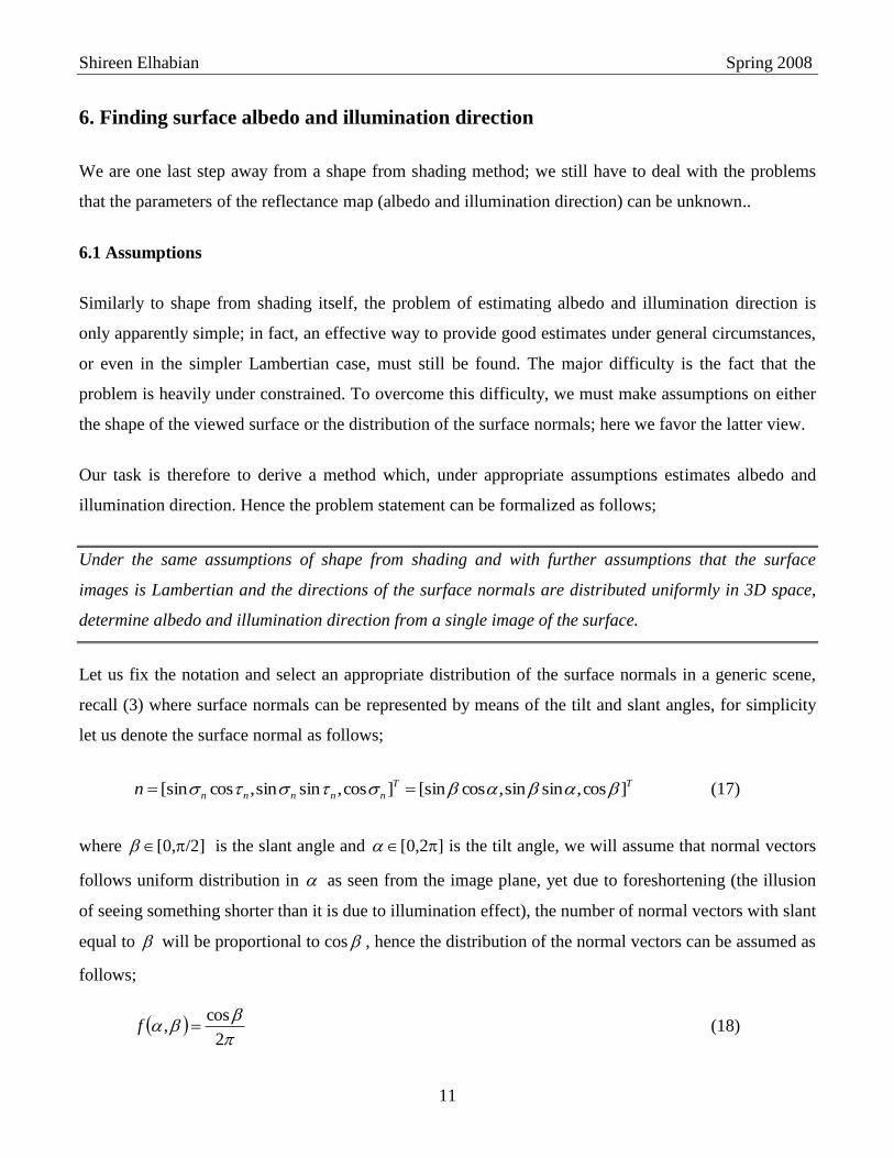
6. Finding surface albedo and illumination direction

We are one last step away from a shape from shading method; we still have to deal with the problems

that the parameters of the reflectance map (albedo and illumination direction) can be unknown..

6.1 Assumptions

Similarly to shape from shading itself, the problem of estimating albedo and illumination direction is

only apparently simple; in fact, an effective way to provide good estimates under general circumstances,

or even in the simpler Lambertian case, must still be found. The major difficulty is the fact that the

problem is heavily under constrained. To overcome this difficulty, we must make assumptions on either

the shape of the viewed surface or the distribution of the surface normals; here we favor the latter view.

Our task is therefore to derive a method which, under appropriate assumptions estimates albedo and

illumination direction. Hence the problem statement can be formalized as follows;

Under the same assumptions of shape from shading and with further assumptions that the surface

images is Lambertian and the directions of the surface normals are distributed uniformly in 3D space,

determine albedo and illumination direction from a single image of the surface.

Let us fix the notation and select an appropriate distribution of the surface normals in a generic scene,

recall (3) where surface normals can be represented by means of the tilt and slant angles, for simplicity

let us denote the surface normal as follows;

TT

nnnnnn ]cos,sinsin,cos[sin]cos,sinsin,cos[sin (17)

where [0,/2] is the slant angle and [0,2] is the tilt angle, we will assume that normal vectors

follows uniform distribution in as seen from the image plane, yet due to foreshortening (the illusion

of seeing something shorter than it is due to illumination effect), the number of normal vectors with slant

equal to will be proportional to cos , hence the distribution of the normal vectors can be assumed as

follows;

2

cos, f (18)


12

6.2 Simple method for Lambertian surfaces

This section will discuss a simple method for recovering albedo and illumination direction. We are given

the gray-scale image, under Lambertian assumption, its relation to the surface albedo and surface

illumination is given by (10), representing the illumination direction as I(,) [0,/2] is the slant

angle and [0,2] is the tilt angle, we obtain (7), substituting (7) and (18) in (10), we will have the

image irradiance (captured gray-scale image) expressed in terms of the slant and tilt angles of the

surface normals as follows, taking into consideration that we still assume that the illumination direction

is fixed for the whole image, hence what vary with respect to the image pixels are surface normals;

coscossinsinsinsinsincossincos),( E (19)

Now lets find the first moment of the image irradiance ),( E , which can be defined as follows where

(.) is the expectation operator;

2

0 0

1

2

),(),(),( ddfEE (20)

This integral breaks down into three additive terms, of which t he first two vanish (because the tilt is

integrated over a full period) and the third yields;

cos4

1 (21)

The interesting fact about (21) is that, as we assumed that the surface normals are distributed according

to (18), we can compute 1 as the average of the brightness values of the given image, and hence we

can consider (21) as an equation for albedo and slant.

A similar derivation for the second moment of the image irradiance, which will boil to the average of the

square of the image brightness and can be related to the albedo and slant as follows;

222

0

2/

0

22

2 cos316

1),(),(),( ddfEE (22)

From (21) and (22), we can estimate the surface albedo and slant as follows;


13

2

12

2 486 (23)

2

12

2

1

486

4cos

(24)

We are still left with the problem of estimating the tilt of the illumination, this can be obtained from

the spatial derivates of the image brightness, Ex and Ey which entails the illumination tilt direction, the

tilt angle can be obtained as follows; refer to [4] for analytical proof of (25).

)(

)(tan

x

y

Eaverage

Eaverage (25)

Hence we can now summarize the method of estimating the surface albedo and illumination direction as

follows; given an intensity image of a Lambertian surface:

Step 1:

Compute the average of the image brightness 1 and of its square 2 , we will use the image we

have just generated to compare our results with the groundtruth parameters used in the image

generation.

% read the image E = double(imread('sphere.jpg'));

% normalizing the image to have maximum of one E = E ./ max(E(:));

% compute the average of the image brightness Mu1 = mean(E(:));

% compute the average of the image brightness square Mu2 = mean(mean(E.^2));

Step 2:

Compute the spatial image gradients in x and y directions. Then we normalize them to have unit

vectors.


14

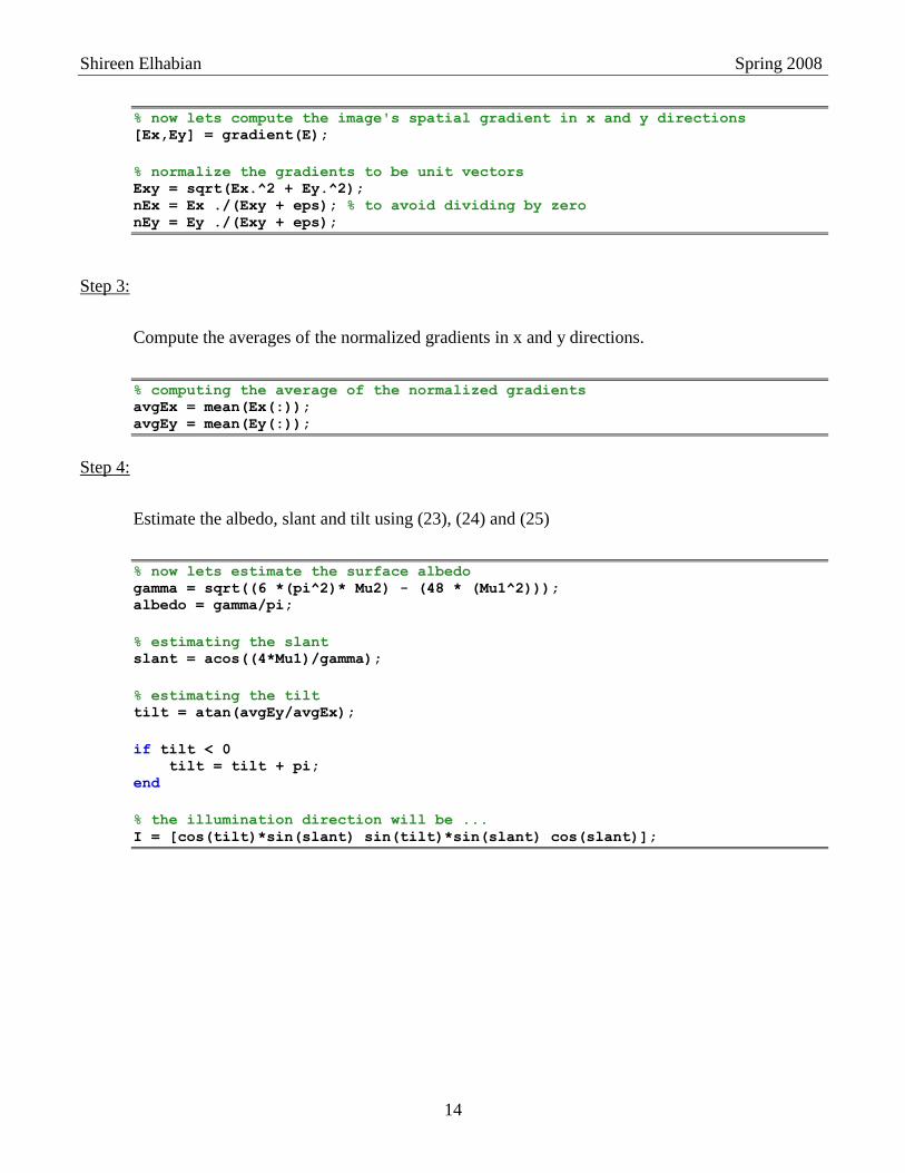
% now lets compute the image's spatial gradient in x and y directions [Ex,Ey] = gradient(E);

% normalize the gradients to be unit vectors Exy = sqrt(Ex.^2 + Ey.^2); nEx = Ex ./(Exy + eps); % to avoid dividing by zero nEy = Ey ./(Exy + eps);

Step 3:

Compute the averages of the normalized gradients in x and y directions.

% computing the average of the normalized gradients avgEx = mean(Ex(:)); avgEy = mean(Ey(:));

Step 4:

Estimate the albedo, slant and tilt using (23), (24) and (25)

% now lets estimate the surface albedo gamma = sqrt((6 *(pi^2)* Mu2) - (48 * (Mu1^2))); albedo = gamma/pi;

% estimating the slant slant = acos((4*Mu1)/gamma);

% estimating the tilt tilt = atan(avgEy/avgEx);

if tilt < 0 tilt = tilt + pi; end

% the illumination direction will be ... I = [cos(tilt)*sin(slant) sin(tilt)*sin(slant) cos(slant)];


15

The computed parameters are :

albedo = 1.0154, slant = 1.0141 , tilt = 0.0131, I = [0.8489 0.0111 0.5284]

Figure 4 – Image gradients in x and y directions and their normalization

As noted by [1], this method gives reasonably good results, though it fails for very small and very large

slants.

You can use images shown in figure 4 and report the results of this algorithm and comment on your

results.


16

Figure 5 – Classical images in shape from shading literature

7. Shape from shading as a minimization problem

We are now ready to search for a solution to the shape from shading problem. Even under the

simplifying Lambertian assumption, the direct inversion of (10) to solve for surface normals is a very

difficult task, which involves the solution of a nonlinear partial differential equation in the presence of

uncertain boundary conditions. Moreover a slight amount of noise in the image can cause (a) non-

existing solution (b) not unique solution or (c) a solution that does not depend continuously on the data.

Hence we are not looking for an exact solution for (10), instead we are seeking an approximation in

some sense.

In literature, shape from shading algorithms can be classified into global and local approaches, where in

global approaches; the surface is recovered by minimizing some energy functional over the entire image.

On the other hand, the local approaches make use of local brightness information to recover surface

patches and then glue them together to obtain the whole surface.

From another perspective, the shape from shading algorithms can be categorized according to the

method used to solve the image irradiance equation (10). There are approaches that try to recover the

surface by minimizing the error between the two sides of (10), i.e. minimization approaches. A second

class of approaches, called propagation approaches, starts from a set of points where the solution is

known and propagates the shape information to the entire image. The last class includes approaches that

reduce the complexity of the problem by either converting the nonlinear image irradiance equation into a

linear one (linear approaches) or by approximating the surface locally by simple shapes (local shading

analysis approaches). In what follows we will concentrate on minimization techniques.


17

7.1 The functional to be minimized

In minimization approaches, the solution of the shape from shading problem is obtained by minimizing

an energy function over the entire image. Two aspects should be considered in this class of approaches:

(1) the choice of the functions which has to be minimized, (2) the method of minimization. In order to

have a unique solution, the functional should be constrained in different ways. In what follows we will

discuss the most important constraints used.

The brightness constraint is the most important constraint. The main idea is to solve for surface normals,

such that when you use these normals with the given surface albedo and illumination direction, you can

form the corresponding 2D image using the image irradiance equation (10), hence we want to find the

surface normals such that there is a minimum deviation from the original given image and the formed

image, this constraint can be defined as follows;

dxdyqpRyxE2

1 ),(),( (26)

where E(x,y) is the given image and R(p,q) is the computed image using the estimated surface normals.

The smoothness constraint is used to obtain a smooth surface that is free from discontinuities, hence the

smoothness constraint can be expressed in terms of the second derivatives of surface normals to ensure

surface smoothness as follows;

dxdyqpqp

dxdyxy

Z

yx

Z

y

Z

x

Z

xyyx

2222

22

22

2

2

22

2

2

2 (27)

Hence the energy function to be minimized can be formulated to minimize the brightness deviation

between the original image and the estimated one, and enforce a smoothness constraint, one possible

way to implement this idea is to look for the minimum of the following functional;

dxdyqpqpqpRyxEdxdy yyxx )()),(),(( 22222

21 (28)


18

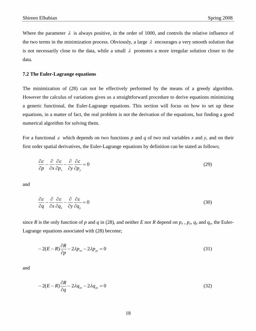
Where the parameter is always positive, in the order of 1000, and controls the relative influence of

the two terms in the minimization process. Obviously, a large encourages a very smooth solution that

is not necessarily close to the data, while a small promotes a more irregular solution closer to the

data.

7.2 The Euler-Lagrange equations

The minimization of (28) can not be effectively performed by the means of a greedy algorithm.

However the calculus of variations gives us a straightforward procedure to derive equations minimizing

a generic functional, the Euler-Lagrange equations. This section will focus on how to set up these

equations, in a matter of fact, the real problem is not the derivation of the equations, but finding a good

numerical algorithm for solving them.

For a functional which depends on two functions p and q of two real variables x and y, and on their

first order spatial derivatives, the Euler-Lagrange equations by definition can be stated as follows;

0

yx pypxp

(29)

and

0

yx qyqxq

(30)

since R is the only function of p and q in (28), and neither E nor R depend on px , py, qx and qy, the Euler-

Lagrange equations associated with (28) become;

022)(2

yyxx pp

p

RRE (31)

and

022)(2

yyxx qq

q

RRE (32)


19

which can be simplified to give;

p

RERp

)(

12

(33)

q

RERq

)(

12

(34)

Where yyxx ppp 2 and yyxx qqq 2 are the Laplacians of p and q respectively. Our next task

now is to solve (33) and (34) for p and q.

7.3 From the continuous to the discrete case

Since the given image is already discrete, we need somehow to find a way to solve (33) and (34) in a

discrete way. We start by denoting pi,j and qi,j as the samples of p and q over the pixel grid at the location

(i,j). Using the formula for the numerical approximation of the second derivative, (33) and (34) become ;

p

RjiEqpRppppp jijijijijijiji

,,

14 ,,1,1,,1,1,

(35)

and

q

RjiEqpRqqqqq jijijijijijiji

,,

14 ,,1,1,,1,1,

(36)

Now the problem is reduced to finding the gradients pi,j and qi,j and hence determining the unknown

surface Z = Z(x,y) from them.

7.4 The algorithm

These equations can be described in the discrete form as:

p

RREpp jiji

)(

4

1,,

(37)

and

q

RREqq jiji

)(

4

1,,

(38)


20

Where jip , and jiq , are the averages of pi,j and qi,j over the four nearest neighbors and are defined as

follows:

4

1,1,,1,1

,

jijijiji

ji

ppppp (39)

and

4

1,1,,1,1

,

jijijiji

ji

qqqqq (40)

An iterative scheme can be used to solve for p and q, starting from some initial configurations for the pi,j

and qi,j, advances from the step k to the step k+1 can be defined according to the following updating

rules;

kkk

p

RREpp

jiji|)(

4

1,,

1

(41)

and

kkk

q

RREqq

jiji|)(

4

1,,

1

(42)

7.5 Enforcing integrability

The solution obtained by iterating (41) and (42) is inconsistent, since the functional was not told that p

and q were the partial derivates of the same function Z, hence there is no Z such that Zx = p and Zy = q.

to overcome this inconvenience, a good idea is to insert a step enforcing integrability after each iteration,

to guarantee that when we integrate p and q we will obtain the surface Z.

The discrete Fourier transform can be used to find the depth Z and enforce the integrability constraint

from the estimated p and q as follows; At each iteration, we compute the Fast Fourier Transform (FFT)

of p and q. Let cp and cq are the Fourier transform of p and q respectively, then

)(

),(yxj

yxpyxecp

(43)


21

)(),(

yxj

yxqyxecq

(44)

Then Z can be computed as the inverse Fourier transform of c(x, y) where:

)(),(

yxj

yxyxecZ

(45)

Such that;

22

)),(),((),(

yx

yxqyyxpx

yx

ccjc

(46)

The function Z in (45) has three important properties;

It provides a solution to the problem of reconstructing a surface from a set of non-integrable p

and q.

Since the coefficients c(x, y) do not depend on x and y, (45) can be easily differentiated with

respect to x and y to give a new set of integrable p and q, say p' and q', such that:

)()(),('),(

yxj

yxp

yxj

yxxyxyx ececj

x

Zp

(47)

and

)()(),('),(

yxj

yxq

yxj

yxyyxyx ececj

y

Zq

(48)

Most importantly, p' and q' are the integrable pair closest to the old pair of p and q.

This can be viewed as if we have projected the old p and q onto a set which contains only integrable

pairs.

7.6 Let’s do it

We now can summarize the algorithm of shape from shading as follows; given the gray-scale image of

the object, do the following;


22

Step 1:

Compute surface albedo and illumination direction using the algorithm described in section 6.

% read the image E = imread('sphere.jpg');

% making sure that it is a grayscale image if isrgb(E) E = rgb2gray(E); end

% downsampling to speedup E = E(1:2:end,1:2:end);

E = double(E);


% first compute the surface albedo and illumination direction ... [albedo,I] = estimate_albedo_illumination (E);

Step 2:

Initializations: surface normals, the second order derivatives of surface normals, the estimated

reflectance map, the controlling parameter λ, the maximum number of iterations, the filter to be

used to get the second order derivates of the surface normals, x in (47) and y in (48) .

% Initializations ... [M,N] = size(E);

% surface normals p = zeros(M,N); q = zeros(M,N);

% the second order derivatives of surface normals p_ = zeros(M,N); q_ = zeros(M,N);

% the estimated reflectance map R = zeros(M,N);

% the controling parameter lamda = 1000;

% maximum number of iterations


23

maxIter = 2000;

% The filter to be used to get the second order derivates of the surface % normals. w = 0.25*[0 1 0;1 0 1;0 1 0]; % refer to equations (39) and (40)

% wx and wy in (47) and (48) [x,y] = meshgrid(1:N,1:M); wx = (2.* pi .* x) ./ M; wy = (2.* pi .* y) ./ N;

Step 3:

Iterate the following steps until a suitable stopping criterion is met;

o Compute the second order derivates of the current surface normals.

o Using the computed surface albedo, illumination direction and surface normals, compute

estimation for the reflectance map.

o Compute the partial derivatives of the reflectance map with respect to p and q.

o Compute the newly estimated surface normals.

o Compute the Fast Fourier Transform of the surface normals.

o Compute the Fourier Transform of the surface Z from the Fourier Transform of the

surface normals.

o Compute the surface Z using inverse Fourier Transform.

o Compute the integrable surface normals.

for k = 1 : maxIter % compute the second order derivates of the surface normals p_ = conv2(p,w,'same'); q_ = conv2(q,w,'same');

% Using the computed surface albedo, illumination direction and % surface normals, compute estimation for the reflectance map.

% refer to (16) R = (albedo.*(-I(1).* p - I(2).* q + I(3)))./sqrt(1 + p.^2 + q.^2);

% Compute the partial derivatives of the reflectance map with respect % to p and q. it will be the differenation of (16) with respect to p % and q pq = (1 + p.^2 + q.^2);

dR_dp =

(-albedo*I(1) ./ (pq .^(1/2))) + (-I(1) * albedo .* p - I(2) * albedo .* q +

I(3) * albedo) .* (-1 .* p .* (pq .^(-3/2)));


24

dR_dq =

(-albedo*I(2) ./ (pq .^(1/2))) + (-I(1) * albedo .* p - I(2) * albedo .* q +

I(3) * albedo) .* (-1 .* q .* (pq .^(-3/2)));

% Compute the newly estimated surface normals ... refer to (41) and % (42) p = p_ + (1/(4*lamda))*(E-R).*dR_dp; q = q_ + (1/(4*lamda))*(E-R).*dR_dq;

% Compute the Fast Fourier Transform of the surface normals. Cp = fft2(p); Cq = fft2(q);

% Compute the Fourier Transform of the surface Z from the Fourier % Transform of the surface normals ... refer to (46) ... C = -i.*(wx .* Cp + wy .* Cq)./(wx.^2 + wy.^2);

% Compute the surface Z using inverse Fourier Transform ... refer to % (45) Z = abs(ifft2(C));

% Compute the integrable surface normals .. refer to (47) and (48) p = ifft2(i * wx .* C); q = ifft2(i * wy .* C);

% saving intermediate results if (mod(k,100) == 0) save(['Z_after_' num2str(k) '_iterations.mat'],'Z'); end end

% visualizing the result figure; surfl(Z);

shading interp;

colormap gray(256);

lighting phong;


25

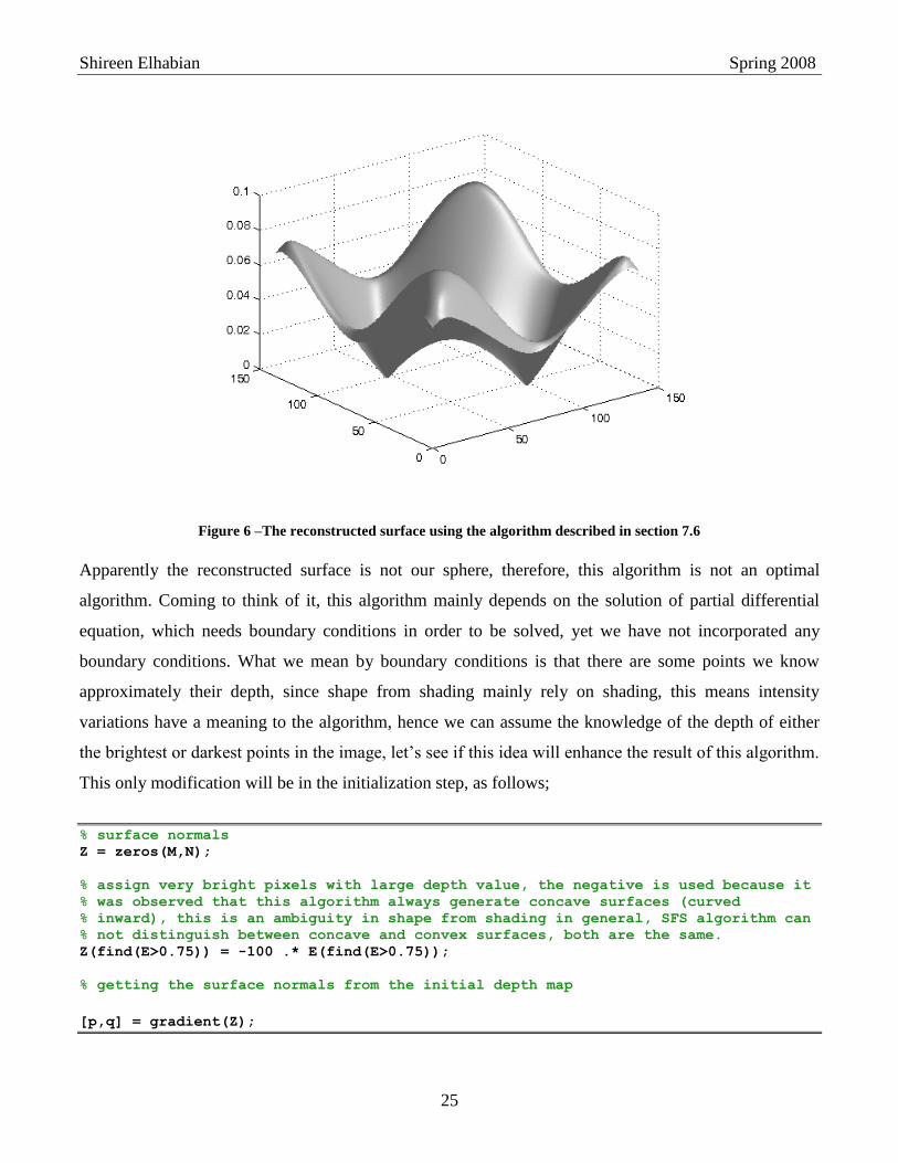
Figure 6 –The reconstructed surface using the algorithm described in section 7.6

Apparently the reconstructed surface is not our sphere, therefore, this algorithm is not an optimal

algorithm. Coming to think of it, this algorithm mainly depends on the solution of partial differential

equation, which needs boundary conditions in order to be solved, yet we have not incorporated any

boundary conditions. What we mean by boundary conditions is that there are some points we know

approximately their depth, since shape from shading mainly rely on shading, this means intensity

variations have a meaning to the algorithm, hence we can assume the knowledge of the depth of either

the brightest or darkest points in the image, let’s see if this idea will enhance the result of this algorithm.

This only modification will be in the initialization step, as follows;

% surface normals Z = zeros(M,N);

% assign very bright pixels with large depth value, the negative is used because it

% was observed that this algorithm always generate concave surfaces (curved

% inward), this is an ambiguity in shape from shading in general, SFS algorithm can

% not distinguish between concave and convex surfaces, both are the same.

Z(find(E>0.75)) = -100 .* E(find(E>0.75));

% getting the surface normals from the initial depth map

[p,q] = gradient(Z);


26

Figure 7 –The reconstructed surface using the algorithm described in section 7.6 after imposing the boundary

conditions

Obviously this result is much better, yet there are other algorithms which lead to more accurate results.

Just out of curiosity, let’s experiment this algorithm on another image.

Figure 8 – another image to experiment the algorithm described in this section.


27

Figure 9 –the reconstructed mug without imposing the boundary conditions

Figure 10 - the reconstructed mug with imposing the boundary conditions

Let us now discuss other types of algorithms which will recover our sphere. You can experiment other

values for illumination direction to discover the cases where this algorithm yields acceptable results.


28

8. Linear approaches

Linear approaches reduce the non-linear problem into a linear through the linearization of the image

irradiance equation (10). The idea is based on the assumption that the lower order components in the

reflectance map dominate. Therefore, these algorithms only work well under this assumption.

8.1 Pentland [6] approach

Under the assumptions of Lambertian surface, orthographic projections, the surface being illuminated by

distant light sources, and the surface is not self-shadowing, Pentland [6] defined the image irradiance

equation as follows;

2222 1

cossinsincossin

1),(),(

qp

qp

qp

iqipiqpRyxE

zyx

(49)

Comparing (46) with (10), we can conclude the following;

It is assumed that the surface has constant albedo, hence it can be ignored as it is not a function

of surface points anymore.

In (10) the surface normal is obtained from the cross product (1,0,p)x(0,1,q), yet in (46) the cross

product is applied in the inverse way, i.e. (0,1,q)x(1,0,p), hence the normal vector becomes (p,q,-

1) instead of (-p,-q,1).

Moreover when using the representation of the illumination direction in terms of its slant and tilt,

the negative sign in (p,q,-1) is ignored since )cos(cos .

By taking the Taylor series expansion of (49) about p = po and q = qo, and ignoring the higher order

terms, the image irradiance equation will be reduced to;

),()(),()(),(),(),( 00000000 qpq

Rqqqp

p

RppqpRqpRyxE

(50)

For Lambertian surface, the above equation at p0 = q0 = 0 reduces to;

sinsinsincoscos),( qpyxE (51)


29

Next, Pentland takes the Fourier transform of both sides of (51). Since the first term on the right is a DC

term, i.e. constant with respect to the variables we are looking for (surface normals), it can be dropped.

Using Fourier transform identities, we have the following;

yxZx FjyxZ

xp ,),(

(52)

yxZy FjyxZy

q ,),(

(53)

Where Fz is the Fourier transform of Z(x,y), taking the Fourier transform of (51), we will get the

following;

sinsin,sincos, yxZyyxZxE FjFjF (54)

Where FE is the Fourier transform of the given image E(x,y). The depth map (our sought surface) Z(x,y)

can be computed by rearranging the terms in (54), and then taking the inverse Fourier transform as

follows;

sinsinsincos,

sinsinsincos,

yx

EyxZ

yxyxZE

jj

FF

jjFF

(55)

Hence,

yxZFyxZ ,),( 1 (56)

This algorithm gives a non-iterative, closed-form solution using Fourier transform. The problem lies in

the linear approximation of the reflectance map, which causes trouble when the non-linear terms are

dominant. As pointed out by Pentland, when the quadratic terms in the reflectance map dominate, the

frequency doubling occurs, in this case, the recovered surface will not be consistent with the

illumination conditions.

Let’s do it …

We now can summarize the algorithm of shape from shading using Pentland approach as follows; given

the gray-scale image of the object, do the following;


30

Step 1:




E = double(E);


% first compute the surface albedo and illumination direction ... [albedo,I,slant,tilt] = estimate_albedo_illumination (E);

Step 2:

Compute the Fourier transform of the given image.

% compute the fourier transform of the image Fe = fft2(E);

Step 3:

Compute x in (47) and y in (48) .

% wx and wy in (47) and (48)

[M,N] = size(E); [x,y] = meshgrid(1:N,1:M); wx = (2.* pi .* x) ./ M; wy = (2.* pi .* y) ./ N;

Step 4:

Using the estimated illumination direction, compute (55).

% Using the estimated illumination direction, compute (55). Fz =


31

Fe./(-i.*wx.*cos(tilt).*sin(slant)-i.*wy.*sin(tilt).*sin(slant));

Step 5:

Compute the inverse Fourier transform to recover the surface and visualize the results.

% Compute the inverse Fourier transform to recover the surface. Z = abs(ifft2(Fz));

% visualizing the result figure; surfl(Z); shading interp; colormap gray(256); lighting phong;

Figure 11 - Surface recovered using Pentland approach

It is obvious that somehow, it is our sphere, yet we are still eager to recover a sphere-like surface not just

a dome as in Fig.7. Hence we will discuss the work of Shah[7] in the next section.


32

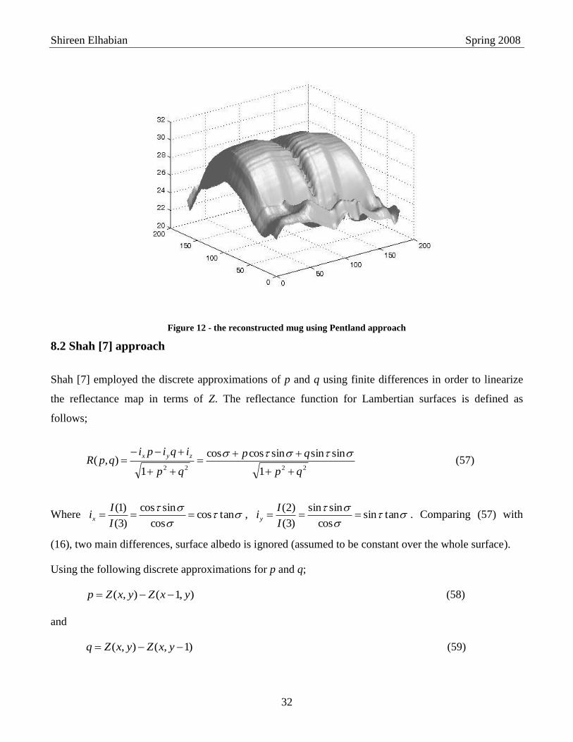
Figure 12 - the reconstructed mug using Pentland approach

8.2 Shah [7] approach

Shah [7] employed the discrete approximations of p and q using finite differences in order to linearize

the reflectance map in terms of Z. The reflectance function for Lambertian surfaces is defined as

follows;

2222 1

sinsinsincoscos

1),(

qp

qp

qp

iqipiqpR

zyx

(57)

Where

tancos

cos

sincos

)3(

)1(

I

Iix ,

tansin

cos

sinsin

)3(

)2(

I

Iiy . Comparing (57) with

(16), two main differences, surface albedo is ignored (assumed to be constant over the whole surface).

Using the following discrete approximations for p and q;

),1(),( yxZyxZp (58)

and

)1,(),( yxZyxZq (59)


33

Shah linearized the function f = E – R = 0 in terms of Z in the vicinity of Zk-1

which is the surface

recovered in iteration k-1. For a fixed point (x,y) and a given image E, a linear approximation (using

Taylor series expansion up through the first order terms) of the function f about a given depth map 1kZ .

For an N by N image, there are N2 such equations, which will form a linear system. This system can be

solved easily using the Jacobi iterative scheme, which simplifies the Taylor series expansion up to the

first order of f into the following equation;

),(

)),(()),(),(()),((0)),((

111

yxdZ

yxZdfyxZyxZyxZfyxZf

nnn

(60)

Let Zn(x,y)= Z (x,y) then

),(

)),((

)),((),(),(

1

11

yxdZ

yxZdf

yxZfyxZyxZ

n

nnn

(61)

where,

222222322

1

1)1(

)(

1)1(

)1)((

),(

)),((

yx

yx

yx

yxn

iiqp

ii

iiqp

qipiqp

yxdZ

yxZdf

(62)

Assuming Z0(x,y) = 0, then Z(x,y) can be extracted iteratively from (61).

Let’s do it …

We now can summarize the algorithm of shape from shading using Shah approach as follows; given the

gray-scale image of the object, do the following;

Step 1:





34

E = double(E);

% first compute the surface albedo and illumination direction ... [albedo,I,slant,tilt] = estimate_albedo_illumination (E);

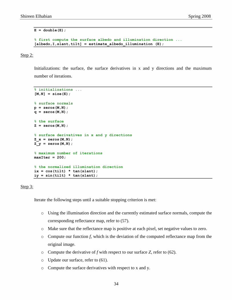
Step 2:

Initializations: the surface, the surface derivatives in x and y directions and the maximum

number of iterations.

% initializations ... [M,N] = size(E);

% surface normals p = zeros(M,N); q = zeros(M,N);

% the surface Z = zeros(M,N);

% surface derivatives in x and y directions Z_x = zeros(M,N); Z_y = zeros(M,N);

% maximum number of iterations maxIter = 200;

% the normalized illumination direction ix = cos(tilt) * tan(slant); iy = sin(tilt) * tan(slant);

Step 3:

Iterate the following steps until a suitable stopping criterion is met:

o Using the illumination direction and the currently estimated surface normals, compute the

corresponding reflectance map, refer to (57).

o Make sure that the reflectance map is positive at each pixel, set negative values to zero.

o Compute our function f, which is the deviation of the computed reflectance map from the

original image.

o Compute the derivative of f with respect to our surface Z, refer to (62).

o Update our surface, refer to (61).

o Compute the surface derivatives with respect to x and y.


35

o Using the updated surface, compute new surface normals, refer to (58) and (59).

for k = 1 : maxIter % using the illumination direction and the currently estimate % surface normals, compute the corresponding reflectance map. % refer to (57) ... R =

(cos(slant) + p .* cos(tilt)*sin(slant)+ q .*

sin(tilt)*sin(slant))./sqrt(1 + p.^2 + q.^2);

% at each iteration, make sure that the reflectance map is positive at % each pixel, set negative values to zero. R = max(0,R);

% compute our function f which is the deviation of the computed % reflectance map from the original image ... f = E - R;

% compute the derivative of f with respect to our surface Z ... refer % to (62) df_dZ =

(p+q).*(ix*p + iy*q + 1)./(sqrt((1 + p.^2 + q.^2).^3)*

sqrt(1 + ix^2 + iy^2))-(ix+iy)./(sqrt(1 + p.^2 + q.^2)*

sqrt(1 + ix^2 + iy^2));

% update our surface ... refer to (61) Z = Z - f./(df_dZ + eps); % to avoid dividing by zero

% compute the surface derivatives with respect to x and y Z_x(2:M,:) = Z(1:M-1,:); Z_y(:,2:N) = Z(:,1:N-1);

% using the updated surface, compute new surface normals, refer to (58) % and (59) p = Z - Z_x; q = Z - Z_y; end

Step 4:

Smooth the obtained surface, then visualize your sphere … see figure (8)

% smoothing the recovered surface Z = medfilt2(abs(Z),[21 21]);

% visualizing the result figure; surfl(Z); shading interp; colormap gray(256);


36

lighting phong;

Figure 13 – Here is our sphere reconstructed using Shah’s approach.

Figure 14 – the reconstructed mug using Shah’s approach.


37

Now

It is your time to experiment all of those algorithms and report your results with your own comments, try

running them on the images in figure (5) and report your results …. Good Luck

References

[1] E. Trucco and A. Verri, Introductory Techniques for 3-D Computer Vision, Prentice Hall Inc., 1998.

[2] B. K. P. Horn, Robot Vision, MIT press, 1986.

[3] Ping-Sing Tsai and Mubarak Shah,”Shape from shading using linear approximation,” Image and

Vision Computing, Vol. 12, No. 8, Oct. 1994, pp 487-498.

[4] Q. Zheng, R. Chellapa, "Estimation of Illuminant Direction, Albedo, and Shape from

Shading," IEEE Transactions on Pattern Analysis and Machine Intelligence ,vol. 13, no. 7, pp. 680-

702, July, 1991.

[5] Emmanuel Prados, Olivier Faugeras , Shape from shading , Handbook of Mathematical Models in

Computer Vision, Springer, page 375--388 – 2006

[6] Pentland, A., "Shape Information From Shading: A Theory About Human Perception," Computer

Vision., Second International Conference on , vol., no., pp.404-413, 5-8 Dec 1988.

[7] P. Tsai and M. Shah. Shape from shading using linear approximation. Image and Vision Computing,

12(8):487--498, 1994.

Hands on Shape from Shading - Scientific …gerig/CS6320-S2015/Materials/Elhabian...To do this,...

Documents

Transcript of Hands on Shape from Shading - Scientific …gerig/CS6320-S2015/Materials/Elhabian...To do this,...