4.  Search Algorithms and Path-finding

Uninformed & informed search, Online search, Robot Path Planning

Alexander Kleiner, Bernhard Nebel

Introduction to Multi-Agent Programming

Contents

•  Problem-Solving Agents •  General Search (Uninformed search) •  Best-First Search (Informed search)

– Greedy Search & A* •  Online Search

– Real-Time Adaptive A* •  Robot Path Planning

–  Sampling Based Planning

Literature

Planning Algorithms

By Steven M. LaValle

Available for downloading at: http://planning.cs.uiuc.edu/

Illustrations and content presented in this lecture where taken from:

Artificial Intelligence – A Modern Approach, 2nd Edition

by Stuart Russell - Peter Norvig

Problem-Solving Agents

  Goal-based agents

Formulation: goal and problem

Given: initial state

Task: To reach the specified goal (a state) through the execution of appropriate actions.

Search for a suitable action sequence and execute the actions

Problem Formulation

•  Goal formulation World states with certain properties

•  Definition of the state space important: only the relevant aspects abstraction

•  Definition of the actions that can change the world state

•  Determination of the search cost (search costs, offline costs) and the execution costs (path costs, online costs)

Note: The type of problem formulation can have a big influence on the difficulty of finding a solution.

Problem Formulation for the Vacuum Cleaner World

•  World state space: 2 positions, dirt or no dirt 8 world states

•  Successor function (Actions): Left (L), Right (R), or Suck (S)

•  Goal state: no dirt in the rooms

•  Path costs: one unit per action

The Vacuum Cleaner State Space

States for the search: The world states 1-8.

Implementing the Search Tree

Data structure for nodes in the search tree:

State: state in the state space

Node: Containing a state, pointer to predecessor, depth, and path cost, action

Depth: number of steps along the path from the initial state

Path Cost: Cost of the path from the initial state to the node

Fringe: Memory for storing expanded nodes. For example, stack or a queue

General functions to implement:

Make-Node(state): Creates a node from a state

Goal-Test(state): Returns true if state is a goal state

Successor-Fn(state): Implements the successor function, i.e. expands a set of new nodes given all actions applicable in the state

Cost(state,action): Returns the cost for executing action in state

Insert(node, fringe): Inserts a new node into the fringe

Remove-First(fringe): Returns the first node from the fringe

General Tree-Search Procedure

Make-Node

Search Strategies

Uninformed or blind searches:

No information on the length or cost of a path to the solution.

• breadth-first search, uniform cost search, depth-first search,

• depth-limited search, Iterative deepening search, and

• bi-directional search

In contrast: informed or heuristic approaches

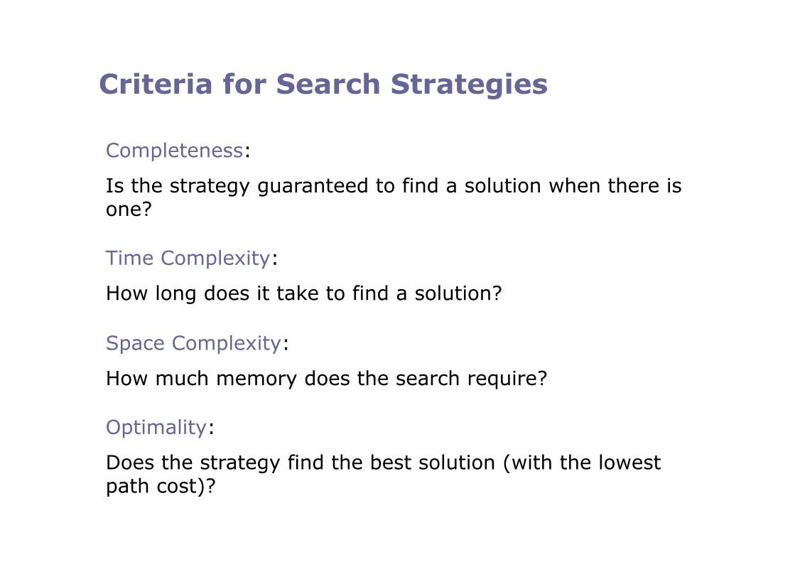
Criteria for Search Strategies

Completeness:

Is the strategy guaranteed to find a solution when there is one?

Time Complexity:

How long does it take to find a solution?

Space Complexity:

How much memory does the search require?

Optimality:

Does the strategy find the best solution (with the lowest path cost)?

Breadth-First Search (1)

Nodes are expanded in the order they were produced . fringe = Enqueue-at-end() (FIFO).

•  Always finds the shallowest goal state first.

•  Completeness.

•  The solution is optimal, provided the path cost is a non-decreasing function of the depth of the node (e.g., when every action has identical, non-negative costs).

Breadth-First Search (2)

The costs, however, are very high. Let b be the maximal branching factor and d the depth of a solution path. Then the maximal number of nodes expanded is

b + b2 + b3 + … + bd + (bd+1 – b) ∈ O(bd+1)

Example: b = 10, 10,000 nodes/second, 1,000 bytes/node:

Depth Nodes Time Memory

2 1,100 .11 seconds 1 megabyte

4 111,100 11 seconds 106 megabytes

6 107 19 minutes 10 gigabytes

8 109 31 hours 1 terabyte

10 1011 129 days 101 terabytes

12 1013 35 years 10 petabytes

14 1015 3,523 years 1 exabyte

Note: One could easily perform the goal test BEFORE expansion, then the time & space complexity reduces to O(bd)

Bidirectional Search

As long as forwards and backwards searches are symmetric, search times of O(2·bd/2) = O(bd/2) can be obtained.

E.g., for b=10, d=6, instead of 111111 only 2222 nodes!

Problems With Repeated States

•  Tree search ignores what happens if nodes are repeatedly visited –  For example, if actions lead back to already visited states –  Consider path planning on a grid

•  Repeated states may lead to a large (exponential) overhead

•  (a) State space with d+1 states, were d is the depth •  (b) The corresponding search tree which has 2d nodes

corresponding to the two possible paths! •  (c) Possible paths leading to A

Graph Search

•  Add a closed list to the tree search algorithm •  Ignore newly expanded state if already in

closed list •  Closed list can be implemented as hash table •  Potential problems

– Needs a lot of memory – Can ignore better solutions if a node is visited

first on a suboptimal path (e.g. IDS is not optimal anymore)

Best-First Search

Search procedures differ in the way they determine the next node to expand.

Uninformed Search: Rigid procedure with no knowledge of the cost of a given node to the goal.

Informed Search: Knowledge of the cost of a given node to the goal is in the form of an evaluation function f or h, which assigns a real number to each node.

Best-First Search: Search procedure that expands the node with the “best” f- or h-value.

General Algorithm

When h is always correct, we do not need to search!

Greedy Search

A possible way to judge the “worth” of a node is to estimate its distance to the goal.

h(n) = estimated distance from n to the goal

The only real condition is that h(n) = 0 if n is a goal.

A best-first search with this function is called a greedy search.

The evaluation function h in greedy searches is also called a heuristic function or simply a heuristic.

In all cases, the heuristic is problem-specific and focuses the search!

Route-finding problem: h = straight-line distance between two locations.

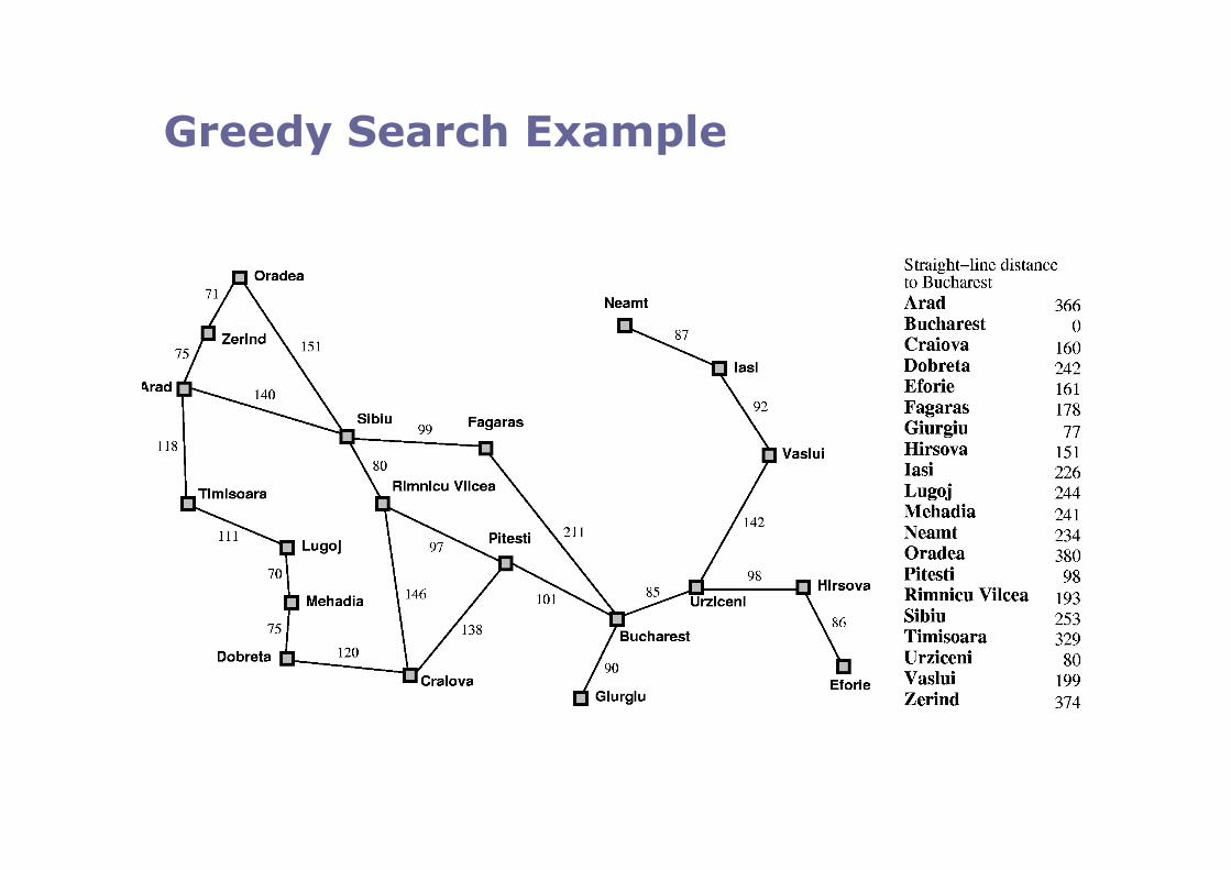
Greedy Search Example

Greedy Search from Arad to Bucharest

However: AradSibiuFagrarasBucharest = 450 AradSibiuRimnicuPitestiBucharest = 418 !

A*: Minimization of the estimated path costs

A* combines the greedy search with the uniform-cost-search, i.e. taking costs into account.

g(n) = actual cost from the initial state to n.

h(n) = estimated cost from n to the next goal.

f(n) = g(n) + h(n), the estimated cost of the cheapest solution through n.

Let h*(n) be the true cost of the optimal path from n to the next goal.

h is admissible if the following holds for all n :

h(n) ≤ h*(n)

We require that for optimality of A*, h is admissible (straight-line distance is admissible).

A* Search Example

A* Search from Arad to Bucharest

f=220+193

=413

Heuristic Function Example

h1 = the number of tiles in the wrong position h2 = the sum of the distances of the tiles from their goal

positions (Manhatten distance)

Empirical Evaluation •  d = distance from goal •  Average over 100 instances •  IDS: Iterative Deepening Search (the best you can do without

any heuristic) # nodes expanded

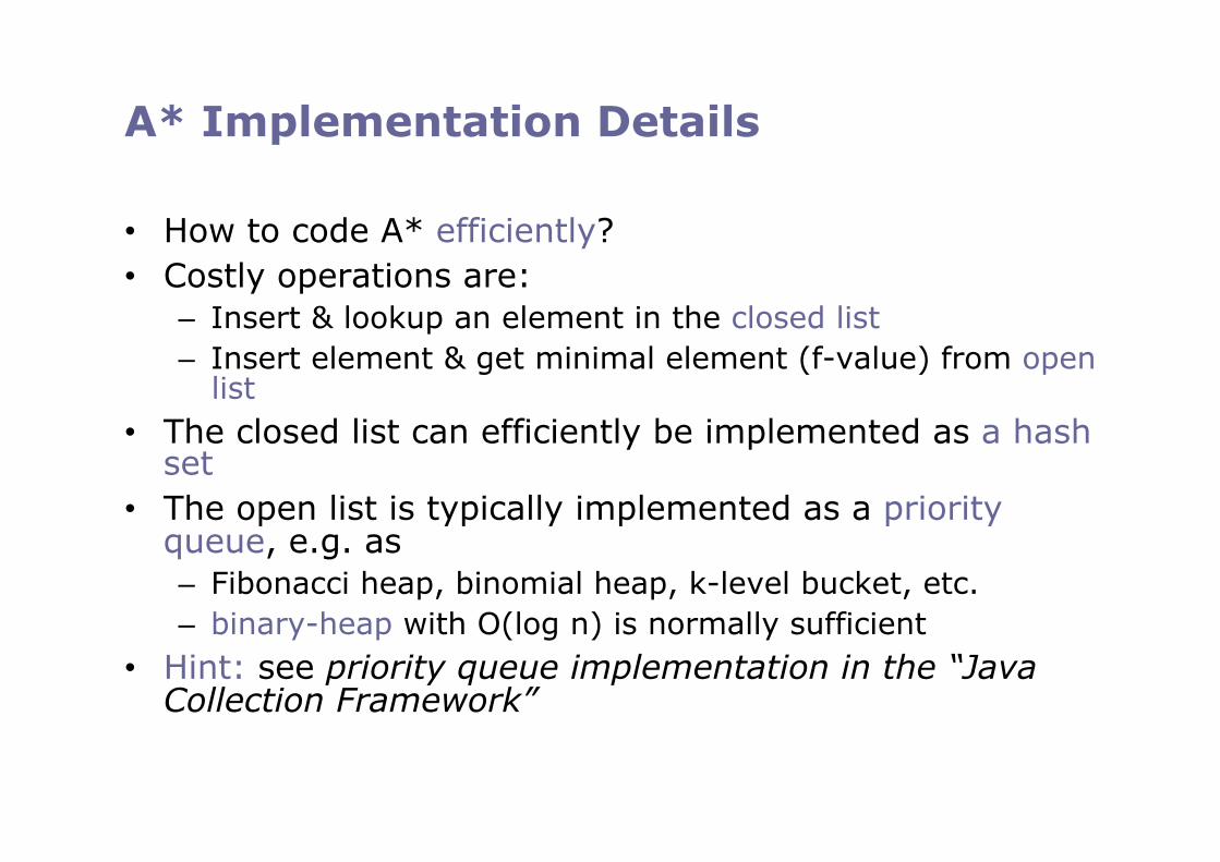
A* Implementation Details

•  How to code A* efficiently? •  Costly operations are:

–  Insert & lookup an element in the closed list –  Insert element & get minimal element (f-value) from open

list •  The closed list can efficiently be implemented as a hash

set •  The open list is typically implemented as a priority

queue, e.g. as –  Fibonacci heap, binomial heap, k-level bucket, etc. –  binary-heap with O(log n) is normally sufficient

•  Hint: see priority queue implementation in the “Java Collection Framework”

Online search

•  Intelligent agents usually don‘t know the state space (e.g. street map) exactly in advance –  Environment can dynamically change! –  True travel costs are experienced during

execution •  Planning and plan execution are interleaved •  Example: RoboCup Rescue

–  The map is known, but roads might be blocked from building collapses

–  Limited drivability of roads depending on traffic volume

•  Important issue: How to reduce computational cost of repeated A* searches!

Online search

•  Incremental heuristic search –  Repeated planning of the complete path from current state to goal –  Planning under the free-space assumption –  Reuse information from previous planning episodes:

•  Focused Dynamic A* (D*) [Stenz95] –  Used by DARPA and NASA

•  D* Lite [Koenig et al. 02] –  Similar as D* but a bit easier to implement (claim)

–  In particular, these methods reuse closed list entries from previous searches

–  All Entries that have been compromised by updates (from observation) are adjusted accordingly

•  Real-Time Heuristic search –  Repeated planning with limited look-ahead (agent centered search) –  Solutions can be suboptimal but faster to compute –  Update of heuristic values of visited states

•  Learning Real-Time A* (LRTA*) [Korf90] •  Real-Time Adaptive A* (RTAA*) [Koenig06]

Real-Time Adaptive A* (RTAA*)

•  Executes A* plan with limited look-ahead

•  Learns better informed heuristic H(s) from experience (initially h(s), e.g. Euclidian distance)

•  Look-ahead defines trade-off between optimality and computational cost

•  astar(lookahead) –  A* expansion as far as

“lookahead” cells and terminates with state s’

while (scurr ∉ GOAL)

astar(lookahead);

if (s’ = FAILURE) then

return FAILURE;

for all s ∈ CLOSED do

H(s) := g(s’)+h(s’)-g(s);

end;

execute(plan); //do one step

end;

return SUCCESS;

s‘: last state expanded during previous A* search

Real-Time Adaptive A* (RTAA*) Example

G S

s‘

s

After first A* planning with look-ahead until s’:

g(s‘)=7, h(s‘)=6, f(s‘)=13

g(s)=2, h(s)=3

Update of each element in CLOSED list, e.g.:

H(s) = g(s‘) + h(s‘) – g(s)

H(s) = 7 + 6 - 2 = 11

Real-Time Adaptive A* (RTAA*) A* vs. RTAA*

A* expansion

RTAA* expansion (inf. Lookahead)

3 8

5 5

h(s)

g(s) f(s)

H(s)

Case Study: ResQ Freiburg path planner Requirements

•  Rescue domain has some special features: –  Interleaving between planning and execution is within

large time cycles –  Roads can be merged into “longroads”

•  Planner is not used only for path finding, also for supporting task assignment –  For example, prefer high utility goals with low path costs –  Hence, planner is frequently called for different goals

•  Our decision: –  Dijkstra graph expansion on longroads –  Collisions are “reduced” by treating other agents on edges

as obstacles (no complete solution)

Case Study: ResQ Freiburg path planner Longroads

•  RoboCup Rescue maps consist of buildings, nodes, and roads –  Buildings are directly connected to nodes –  Roads are inter-connected by crossings

•  For efficient path planning, one can extract a graph of longroads that basically consists of road segments that are connected by crossings

Longroad

Case Study: ResQ Freiburg path planner Approach

•  Reduction of street network to longroad network •  Caching of planning queries (useful if same queries are

repeated) •  Each agent computes two Dijkstra graphs, one for each

nearby longroad node •  Selection of optimal path by considering all 4 possible

plans •  Dijkstra graphs are recomputed after each perception

update (either via direct sensing or communication) •  Additional features:

–  Parameter for favoring unknown roads (for exploration) –  Two more Dijkstra graphs for sampled time cost (allows

time prediction)

Case Study: ResQ Freiburg path planner Dijkstra‘s Algorithm (1)

Single Source Shortest Path, i.e. finds the shortest path from a single node to all other nodes

Worst case runtime O(|E| log |V|), assuming E>V, where E is the set of edges and V the set of vertices

– Requires efficient priority queue

Robot Motion Planning Introduction

A motion computed by a planning algorithm, for a digital actor to reach into a refrigerator

A planning algorithm computes the motions of 100 digital actors moving across terrain with obstacles

An application of motion planning to the sealing process in automotive manufacturing

Robot Motion Planning Introduction

Several mobile robots attempt to successfully navigate in an indoor environment while avoiding collisions with the walls and each other

Using mobile robots to move a piano

Obstacle region

Robot configuration

Suppose world or

Robot Motion Planning Problem Formulation

The configuration space is the space containing all possible configurations of the robot

Rigid robot

Obstacle region is defined by:

Which is the set of all configurations q at which A(q), the transformed robot, intersects

The free space is defined by:

Robot Motion Planning Problem / Solution Concepts

Problem: Find continuous path

With and

•  Requirements –  Shortest path –  Minimal execution time (requiring a good fit with the motion model, least amount of

rotations, etc.) –  Maximal distance to obstacles (needed in dynamic environments, and when

sensors are unreliable) •  Many solution concepts, generally we have

1.  Potential Fields (more details in a later lecture) 2.  Visibility Graphs 3.  Grid-based Planning 4.  Sampling-based Planning

Robot Motion Planning Visibility Graphs

•  Approximation of obstacles as polygons (or circles)

•  Visibility Graph S: Build visibility graph S=(V,G), where V is the set of all vertices from polygon obstacles or circle tangents

•  Planning with discrete methods (e.g. A*)

•  Advantage: Depends only on number of obstacles only

•  Disadvantage: Paths very close to obstacles. How to get good polygons?

Robot Motion Planning Grid-based Planning

•  Planning on a subdivision of Cfree into smaller cells

•  Simplification: grow borders of obstacles up to the diameter of the robot, e.g., by Gaussian blur

•  Construction of graph G=(V,E), where V is the set of cells and E represents their neighbor-relations

•  Planning with discrete methods (e.g. A*)

–  Resulting path is a sequence of cells

•  Hierarchical planning: find path on coarse resolution and re-plan on more fine grained resolutions

•  Disadvantage: Memory usage grows with the size of the environment

•  Advantage: No polygons!

Robot Motion Planning Sampling-based Motion Planning

•  Basic Idea: To avoid explicit construction of Cobs

•  Instead: probe Cfree with a sampling scheme

•  Builds a graph G=(V,E) by connecting sampled locations –  each e ∊ E has to be collision free! –  on G a solution can be found by

discrete search methods (e.g. A*)

•  Critical part: Random Sampling

•  Time consuming part: Collision Checks

Sampling without obstacles

Sampling with obstacles

Sampling-based Motion Planning General Procedure

1.  Initialization:

–  Let G=(V,E) be an undirected search graph with (qstart, qgoal) ∊ V, E =∅

2.  Vertex Selection Method (VSM): –  Select a vertex qcurr ∊ V for expansion

3.  Local Planning Method (LPM): –  Select any qnew∊ Cfree by sampling

–  Find a path τs :[0:1] ➝ Cfree such that τ(0)= qcurr and τ(1)=qnew

–  τs must be collision free, if not, go to 2)

4.  Insert new Vertex & Edge in the Graph: –  Insert edge between qcurr and qnew

–  Insert qnew to V

5.  Check for a Solution: –  Check if there is a valid path on G from qstart to qgoal, if yes: terminate

6.  Return to step 2) until any termination criterion is met

Sampling-based Motion Planning Difficulties

Multi-resolution search required to quickly overcome cavities

Bidirectional search needed in some cases

Sometimes even multi-dimensional search needed

Hard to solve even with multi-dimensional search

Sampling-based Motion Planning Random Sampling / Deterministic Sampling

•  A Sampling sequence should reach every point in C! However, C is uncountably infinite …

•  In practice, sampling has to terminate early. Hence the sequence of sampling matters!

•  Dense Sequence: A sequence getting with increasing size arbitrarily close to every element in C

•  Random sampling: –  Suppose C=[0,1] and I ⊂ C is an interval of length e. If k samples are chosen independently at

random, the probability that none of them falls into I is (1−e)k. As k approaches infinity, this probability converges to zero. This means random sampling is probably dense.

•  Deterministic sampling: –  Suppose C=[0,1] and we want to place 16 samples

–  Simple approach: •  Select the set S={i/16 | 0<i<16} so that all samples are evenly distributed

–  What if we want to make S into a sequence? What is the best ordering? What if 16 points are not enough, i.e., are not reaching every interesting point in C?

–  Problem with “sorting by increasing value”: after i=8 half of C has been neglected! It would be preferable to have a nice covering of C for every i

Sampling-based Motion Planning The Van der Corput sequence

•  Idea: to reverse the order of the bits, when the sequence is represented with binary decimals

•  By reversing the bits, the most significant bit toggles in every step, which means that the sequence alternates between the lower and upper halves of C.

Sequence for i<=16

Note: Both method can also be applied for C⊆ℜm by sampling each dimension independently

Sampling-based Motion Planning Rapidly Exploring Dense Trees (RDTs)

•  Let S(G) be the set of all points reached by G (either vertices or edges) •  Requires a dense sequence α(i) •  Connects iteratively edges from α(i) to those nearest in G

Basic algorithm for RDTs (without obstacles):

q0

qnear

α(i)

q0

qnear

α(i)

Case 1: Nearest point is a vertex

Case 2: Nearest point is on an edge

Result:

Sampling-based Motion Planning Rapidly Exploring Dense Trees (RDTs) Basic algorithm for RDTs (with obstacles):

•  STPPING-CONFIGURATION() returns the nearest configuration possible in Cfree

q0

qnear

α(i) Cobs qs

Bug trap video on YouTube

http://www.youtube.com/watch?v=qci_AktcrD4

Summary

•  A problem consists of five parts: The state space, initial situation, actions, goal test, and path costs. A path from an initial state to a goal state is a solution.

•  Search algorithms are judged on the basis of completeness, optimality, time complexity, and space complexity.

•  Best-first search expands the node with the highest worth (defined by any measure) first.

•  When h(n) is admissible, i.e., h* is never overestimated, we obtain the A* search, which is complete and optimal.

•  Online search provides method that are computationally more efficient when planning and plan execution are tightly coupled

•  Sampling-based Planning methods are well suited for Robot Motion Planning

Literature

•  Homepage of Tony Stentz: –  A. Stentz The focussed D* algorithm for real-time replanning Proc. of the Int.

Join Conference on Artificial Intelligence, p. 1652-1659, 1995.

•  Homepage of Sven Koenig: –  S. Koenig and X. Sun. Comparing Real-Time and Incremental Heuristic

Search for Real-Time Situated Agents Journal of Autonomous Agents and Multi-Agent Systems, 2009

–  S. Koenig and M. Likhachev Real-Time Adaptive A* Proceedings of the International Joint Conference on Autonomous Agents and Multiagent Systems (AAMAS), 281-288, 2006

–  S. Koenig and M. Likhachev. Fast Replanning for Navigation in Unknown Terrain Transactions on Robotics, 21, (3), 354-363, 2005.

•  More difficult to find, also explained in the AIMA book (2nd ed.): –  R. Korf. Real-time heuristic search. Artificial Intelligence, 42(2-3):189-211, 1990.

–  Demo search code in Java on the AIMA webpage http://aima.cs.berkeley.edu/