Stochastic greedy local searchStochastic greedy local search

Chapter 7Chapter 7

ICS-275

Spring 2007

Example: 8-queen problem

Main elements Choose a full assignment and iteratively

improve it towards a solution Requires a cost function: number of unsatisfied

constraints or clasuses. Neural networks use energy minimization

Drawback: local minimas Remedy: introduce a random element Cannot decide inconsistency

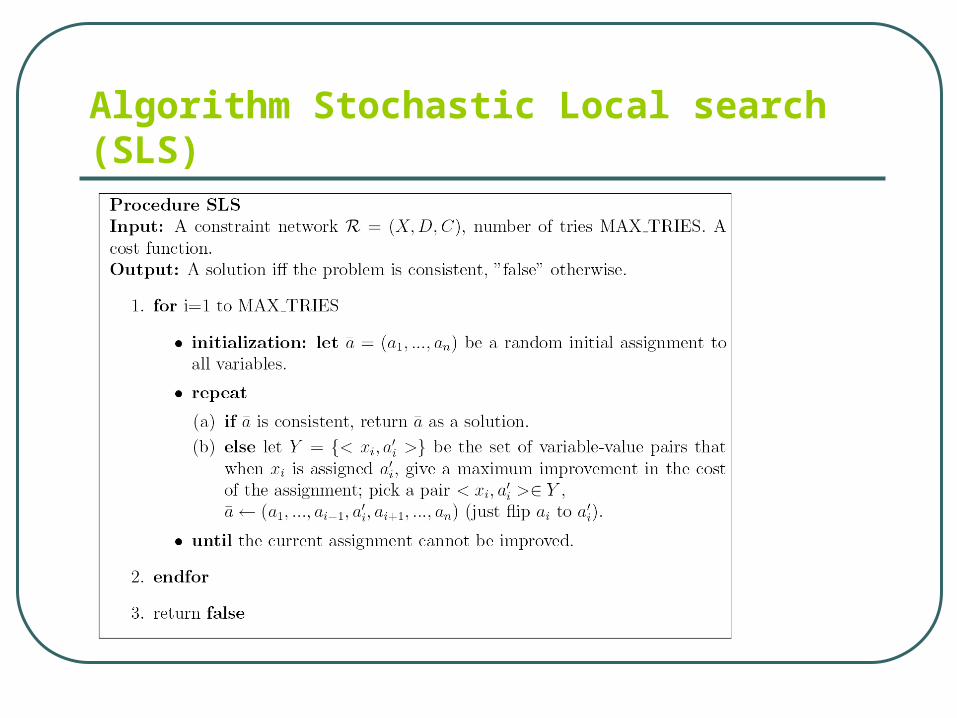
Algorithm Stochastic Local search (SLS)

Example: CNF

Example: z divides y,x,t z = {2,3,5}, x,y = {2,3,4}, t={2,5,6}

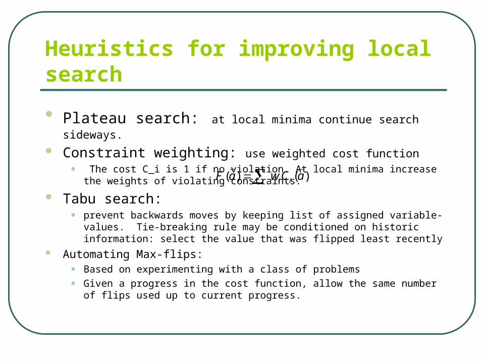
Heuristics for improving local search

Plateau search: at local minima continue search sideways.

Constraint weighting: use weighted cost function

• The cost C_i is 1 if no violation. At local minima increase the weights of violating constraints.

Tabu search: • prevent backwards moves by keeping list of assigned variable-values. Tie-

breaking rule may be conditioned on historic information: select the value that was flipped least recently

Automating Max-flips:

• Based on experimenting with a class of problems

• Given a progress in the cost function, allow the same number of flips used up to current progress.

)()(__

aCwaF ii

Random walk strategies

Combine random walk with greediness• At each step:

• choose randomly an unsatisfied clause.

• with probability p flip a random variable in the clause, with (1-p) do a greedy step minimizing the breakout value: the number of new constraints that are unsatisfied

Figure 7.2: Algorithm WalkSAT

Example of walkSAT: start with assignment of true to all vars

Simulated Annealing (Kirkpatric, Gellat and Vecchi (1983))

Pick a variable and a value and compute delta: the change in the cost function when the variable is flipped to the value.

If change improves execute it, Otherwise it is executed with probablity e^(-delta/T), T

is a temperature parameter. The algorithm will converge if T is reduced gradualy.

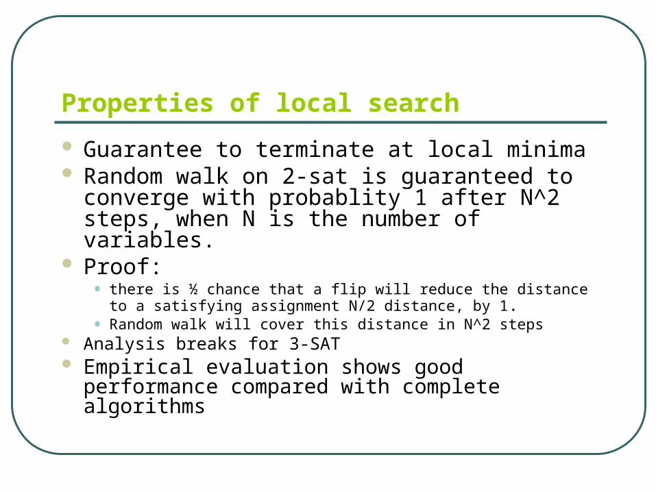
Properties of local search

Guarantee to terminate at local minima Random walk on 2-sat is guaranteed to

converge with probablity 1 after N^2 steps, when N is the number of variables.

Proof: • there is ½ chance that a flip will reduce the distance to a satisfying

assignment N/2 distance, by 1.• Random walk will cover this distance in N^2 steps

Analysis breaks for 3-SAT Empirical evaluation shows good performance

compared with complete algorithms

Hybrids of local search and Inference

We can use exact hybrids of search+inference and replace search by SLS (Kask and Dechter 1996)• Good when cutset is small

The effect of preprocessing by constraint propagation on SLS (Kask and Dechter 1995)• Great improvement on structured problems

• Not so much on uniform problems

Structured (hierarchical 3SAT cluster structures) vs. (uniform) random.

SLS and Local Consistency

Basic scheme : Apply preprocessing (resolution, path consistency) Run SLS Compare against SLS alone

SLS and Local Consistency

SLS and Local Consistency

SLS and Local Consistency

100,8,32/64 100,8,16/64

SLS and Local Consistency

100,8,32/64 100,8,16/64

SLS and Local Consistency

SLS and Local Consistency

For structured problems, enforcing local consistency will improve SLS

For uniform CSPs, enforcing local consistency is not cost effective: performance of SLS is improved, but not enough to compensate for the preprocessing cost.

Summary:

SLS and Cutset Conditioning

Background:

Cycle cutset technique improves backtracking by conditioning only on cutset variables.

}1,0{iX }1,0{jX

cutset

SLS and Cutset Conditioning

Background: Tree algorithm is tractable for trees. Networks with bounded width are tractable*.

Basic Scheme: Identify a cutset such that width is reduced to desired value. Use search with cutset conditioning.

Local search on Cycle-cutset

Y

Tree variables X

Local search on Cycle-cutset

BTBT

SLS

Tree-alg

Tree-alg

SLS

Tree Algorithm

Tree Algorithm (contd)

GSAT with Cycle-Cutset (Kask and Dechter, 1996)

Input: a CSP, a partition of the variables into cycle-cutset and tree variablesOutput: an assignment to all the variables

Within each try:Generate a random initial asignment, and then alternate between the two steps:

1. Run Tree algorithm (arc-consistency+assignment) on the problem with fixed values of cutset variables. 2. Run GSAT on the problem with fixed values of tree variables.

Theorem 7.1

Results: GSAT with Cycle-Cutset(Kask and Dechter, 1996)

Results GSAT with Cycle-Cutset(Kask and Dechter, 1996)

GSAT versus GSAT +CC

0

10

20

30

40

50

60

70

14 22 36 43

cycle cutset size

# o

f p

rob

lem

s s

olv

ed

GSAT

GSAT+CC

SLS and Cutset Conditioning

A new combined algorithm of SLS and inference based on cutset conditioning

Empirical evaluation on random CSPs SLS combined with the tree algorithm is superior to pure SLS

when the cutset is small

Summary:

Possible project

Program variants of SLS+Inference• Use the computed cost on the tree to guide SLS on

the cutset. This is applicable to optimization

• Replace the cost computation on the tree with simple arc-consistency or unit resolution

• Implement the idea for SAT using off-the-shelves code: unit-resolution from minisat, SLS from walksat.

Other projects: start thinking.