Selective Greedy Equivalence Search: Finding Optimal Bayesian NetworksUsing a Polynomial Number of Score Evaluations

David Maxwell ChickeringMicrosoft Research

Redmond, WA 98052dmax@microsoft.com

Christopher MeekMicrosoft Research

Redmond, WA 98052meek@microsoft.com

Abstract

We introduce Selective Greedy EquivalenceSearch (SGES), a restricted version of GreedyEquivalence Search (GES). SGES retains theasymptotic correctness of GES but, unlike GES,has polynomial performance guarantees. In par-ticular, we show that when data are sampled in-dependently from a distribution that is perfectwith respect to a DAG G defined over the ob-servable variables then, in the limit of large data,SGES will identify G’s equivalence class aftera number of score evaluations that is (1) poly-nomial in the number of nodes and (2) expo-nential in various complexity measures includingmaximum-number-of-parents, maximum-clique-size, and a new measure called v-width thatis at least as small as—and potentially muchsmaller than—the other two. More generally,we show that for any hereditary and equivalence-invariant property Π known to hold in G, weretain the large-sample optimality guarantees ofGES even if we ignore any GES deletion oper-ator during the backward phase that results in astate for which Π does not hold in the common-descendants subgraph.

1 INTRODUCTION

Greedy Equivalence Search (GES) is a score-basedsearch algorithm that searches over equivalence classesof Bayesian-network structures. The algorithm is appeal-ing because (1) for finite data, it explicitly (and greedily)tries to maximize the score of interest, and (2) as the datagrows large, it is guaranteed—under suitable distributionalassumptions—to return the generative structure. Althoughempirical results show that the algorithm is efficient in real-world domains, the number of search states that GES needsto evaluate in the worst case can be exponential in the num-ber of domain variables.

In this paper, we show that if we assume the generative dis-tribution is perfect with respect to some DAG G definedover the observable variables, and if G is known to be con-strained by various graph-theoretic measures of complex-ity, then we can disregard all but a polynomial number ofthe backward search operators considered by GES whileretaining the large-sample guarantees of the algorithm; wecall this new variant of GES selective greedy equivalencesearch or SGES. Our complexity results are a consequenceof a new understanding of the backward phase of GES,in which edges (either directed or undirected) are greed-ily deleted from the current state until a local minimum isreached. We show that for any hereditary and equivalence-invariant property known to hold in generative model G,we can remove from consideration any edge-deletion op-erator between X and Y for which the property does nothold in the resulting induced subgraph over X, Y, and theircommon descendants. As an example, if we know that eachnode has at most k parents, we can remove from consider-ation any deletion operator that results in a common childwith more than k parents.

We define a new notion of complexity that we call v-width.For a given generative structure G, v-width is necessarilysmaller than the maximum clique size, which is necessar-ily smaller than or equal to the maximum number of parentsper node. By casting limited v-width and other complexityconstraints as graph properties, we show how to enumeratedirectly over a polynomial number of edge-deletion oper-ators at each step, and we show that we need only a poly-nomial number of calls to the scoring function to completethe algorithm.

The main contributions of this paper are theoretical. Ourdefinition of the new SGES algorithm deliberately leavesunspecified the details of how to implement its forwardphase; we prove our results for SGES given any implemen-tation of this phase that completes with a polynomial num-ber of calls to the scoring function. A naive implementationis to immediately return a complete (i.e., no independence)graph using no calls to the scoring function, but this choiceis unlikely to be reasonable in practice, particularly in dis-

crete domains where the sample complexity of this initialmodel will likely be a problem. Whereas we believe it animportant direction, our paper does not explore practical al-ternatives for the forward phase that have polynomial-timeguarantees.

This paper, which is an expanded version of Chickering andMeek (2015) and includes all proofs, is organized as fol-lows. In Section 2, we describe related work. In Section 3,we provide notation and background material. In Section 4,we present our new SGES algorithm, we show that it is op-timal in the large-sample limit, and we provide complexitybounds when given an equivalence-invariant and hereditaryproperty that holds on the generative structure. In Section5, we present a simple synthetic experiment that demon-strates the value of restricting the backward operators inSGES. We conclude with a discussion of our results in Sec-tion 6.

2 RELATED WORK

It is useful to distinguish between approaches to learn-ing the structure of graphical models as constraint based,score based or hybrid. Constraint-based approaches typi-cally use (conditional) independence tests to eliminate po-tential models, whereas score-based approaches typicallyuse a penalized likelihood or a marginal likelihood to eval-uate alternative model structures; hybrid methods combinethese two approaches. Because score-based approaches aredriven by a global likelihood, they are less susceptible thanconstraint-based approaches to incorrect categorical deci-sions about independences.

There are polynomial-time algorithms for learning the bestmodel in which each node has at most one parent. Inparticular, the Chow-Liu algorithm (Chow and Liu, 1968)used with any equivalence-invariant score will identifythe highest-scoring tree-like model in polynomial time;for scores that are not equivalence invariant, we can usethe polynomial-time maximum-branching algorithm of Ed-monds (1967) instead. Gaspers et al. (2012) show how tolearn k-branchings in polynomial time; these models arepolytrees that differ from a branching by a constant k num-ber of edge deletions.

Without additional assumptions, most results for learningnon-tree-like models are negative. Meek (2001) shows thatfinding the maximum-likelihood path is NP-hard, despitethis being a special case of a tree-like model. Dasgupta(1999) shows that finding the maximum-likelihood poly-tree (a graph in which each pair of nodes is connectedby at most one path) is NP-hard, even with bounded in-degree for every node. For general directed acyclic graphs,Chickering (1996) shows that finding the highest marginal-likelihood structure under a particular prior is NP-hard,even when each node has at most two parents. Chicker-ing at al. (2004) extend this same result to the large-sample

case.

Researchers often assume that the training-data “genera-tive” distribution is perfect with respect to some modelclass in order to reduce the complexity of learning algo-rithms. Geiger et al. (1990) provide a polynomial-timeconstraint-based algorithm for recovering a polytree un-der the assumption that the generative distribution is per-fect with respect to a polytree; an analogous score-basedresult follows from this paper. The constraint-based PCalgorithm of Sprites et al. (1993) can identify the equiva-lence class of Bayesian networks in polynomial time if thegenerative structure is a DAG model over the observablevariables in which each node has a bounded degree; thispaper provides a similar result for a score-based algorithm.Kalish and Buhlmann (2007) show that for Gaussian dis-tributions, the PC algorithm can identify the right structureeven when the number of nodes in the domain is larger thanthe sample size. Chickering (2002) uses the same DAG-perfectness-over-observables assumption to show that thegreedy GES algorithm is optimal in the large-sample limit,although the branching factor of GES is worst-case expo-nential; the main result of this paper shows how to limitthis branching factor without losing the large-sample guar-antee. Chickering and Meek (2002) show that GES iden-tifies a “minimal” model in the large-sample limit under aless restrictive set of assumptions.

Hybrid methods for learning DAG models use a constraint-based algorithm to prune out a large portion of the searchspace, and then use a score-based algorithm to selectamong the remaining (Friedman et al., 1999; Tsamardinoset al., 2006). Ordyniak and Szeider (2013) give positivecomplexity results for the case when the remaining DAGsare characterized by a structure with constant treewidth.

Many researchers have turned to exhaustive enumerationto identify the highest-scoring model (Gillispie and Perl-man, 2001; Koivisto and Sood 2004; Silander and Myl-lymaki, 2006; Kojima et al, 2010). There are many com-plexity results for other model classes. Karger and Sre-bro (2001) show that finding the optimal Markov net-work is NP-complete for treewidth > 1. Narasimhan andBilmes (2004) and Shahaf, Chechetka and Guestrin (2009)show how to learn approximate limited-treewidth models inpolynomial time. Abeel, Koller and Ng (2005) show howto learn factor graphs in polynomial time.

3 NOTATION AND BACKGROUND

We use the following syntactical conventions in this paper.We denote a variable by an upper case letter (e.g., A) anda state or value of that variable by the same letter in lowercase (e.g., a). We denote a set of variables by a bold-facecapitalized letter or letters (e.g., X). We use a correspond-ing bold-face lower-case letter or letters (e.g., x) to denotean assignment of state or value to each variable in a given

set. We use calligraphic letters (e.g., G, E) to denote statis-tical models and graphs.

A Bayesian-network model for a set of variables U is a pair(G,θ). G = (V,E) is a directed acyclic graph—or DAGfor short—consisting of nodes in one-to-one correspon-dence with the variables and directed edges that connectthose nodes. θ is a set of parameter values that specify allof the conditional probability distributions. The Bayesiannetwork represents a joint distribution over U that factorsaccording to the structure G.

The structure G of a Bayesian network represents the inde-pendence constraints that must hold in the distribution. Theset of all independence constraints implied by the structureG can be characterized by the Markov conditions, whichare the constraints that each variable is independent of itsnon-descendants given its parents. All other independenceconstraints follow from properties of independence. A dis-tribution defined over the variables from G is perfect withrespect to G if the set of independences in the distribution isequal to the set of independences implied by the structureG.

Two DAGs G and G′ are equivalent1—denoted G ≈ G′—ifthe independence constraints in the two DAGs are identi-cal. Because equivalence is reflexive, symmetric, and tran-sitive, the relation defines a set of equivalence classes overnetwork structures. We will use [G]≈ to denote the equiva-lence class of DAGs to which G belongs.

An equivalence class of DAGs F is an independence map(IMAP) of another equivalence class of DAGs E if all in-dependence constraints implied by F are also implied byE . For two DAGs G and H, we use G ≤ H to denote that[H]≈ is an IMAP of [G]≈; we use G < H when G ≤ H and[H]≈ 6= [G]≈.

As shown by Verma and Pearl (1991), two DAGs areequivalent if and only if they have the same skeleton (i.e.,the graph resulting from ignoring the directionality of theedges) and the same v-structures (i.e., pairs of edges X →Y and Y ← Z where X and Z are not adjacent). Asa result, we can use a partially directed acyclic graph—or PDAG for short—to represent an equivalence class ofDAGs: for a PDAG P , the equivalence class of DAGs isthe set that share the skeleton and v-structures with P2.

We extend our notation for DAG equivalence and the DAGIMAP relation to include the more general PDAG structure.In particular, for a PDAG P , we use [P]≈ to denote thecorresponding equivalence class of DAGs. For any pair ofPDAGs P and Q—where one or both may be a DAG—we

1We make the standard conditional-distribution assumptionsof multinomials for discrete variables and Gaussians for contin-uous variables so that if two DAGs have the same independenceconstraints, then they can also model the same set of distributions.

2The definitions for the skeleton and set of v-structures for aPDAG are the obvious extensions to these definitions for DAGs.

use P ≈ Q to denote [Q]≈ = [P]≈ and we use P ≤ Q todenote [Q]≈ is an IMAP of [P]≈. To avoid confusion, forthe remainder of the paper we will reserve the symbols GandH for DAGs.

For any PDAG P and subset of nodes V, we use P[V] todenote the subgraph of P induced by V; that is, P[V] hasas nodes the set V and has as edges all those from P thatconnect nodes in V. We use NAX,Y to denote, withina PDAG, the set of nodes that are neighbors of X (i.e.,connected with an undirected edge) and also adjacent toY (i.e., without regard to whether the connecting edge isdirected or undirected).

An edge in G is compelled if it exists in every DAG thatis equivalent to G. If an edge in G is not compelled, wesay that it is reversible. A completed PDAG (CPDAG) Cis a PDAG with two additional properties: (1) for every di-rected edge in C, the corresponding edge in G is compelledand (2) for every undirected edge in C the correspondingedge in G is reversible. Unlike non-completed PDAGs, theCPDAG representation of an equivalence class is unique.We use PaPY to denote the parents of node Y in P . Anedge X → Y is covered in a DAG if X and Y have thesame parents, with the exception that X is not a parent ofitself.

3.1 Greedy Equivalence Search

Algorithm GES(D)

Input : Data DOutput: CPDAG CC ←− FES(D)C ←− BES(D, C)return C

Figure 1: Pseudo-code for the GES algorithm.

The GES algorithm, shown in Figure 1, performs a two-phase greedy search through the space of DAG equivalenceclasses. GES represents each search state with a CPDAG,and performs transformation operators to this representa-tion to traverse between states. Each operator correspondsto a DAG edge modification, and is scored using a DAGscoring function that we assume has three properties. First,we assume the scoring function is score equivalent, whichmeans that it assigns the same score to equivalent DAGs.Second, we assume the scoring function is locally consis-tent, which means that, given enough data, (1) if the cur-rent state is not an IMAP of G, the score prefers edge ad-ditions that remove incorrect independences, and (2) if thecurrent state is an IMAP of G, the score prefers edge dele-tions that remove incorrect dependences. Finally, we as-sume the scoring function is decomposable, which means

we can express it as:

Score(G,D) =

n∑i=1

Score(Xi,PaGi ) (1)

Note that the data D is implicit in the right-hand side Equa-tion 1. Most commonly used scores in the literature havethese properties. For the remainder of this paper, we as-sume they hold for the scoring function we use.

All of the CPDAG operators from GES are scored usingdifferences in the DAG scoring function, and in the limit oflarge data, these scores are positive precisely for those op-erators that remove incorrect independences and incorrectdependences.

The first phase of the GES—called forward equivalencesearch or FES—starts with an empty (i.e., no-edge)CPDAG and greedily applies GES insert operators until nooperator has a positive score; these operators correspondprecisely to the union of all single-edge additions to allDAG members of the current (equivalence-class) state. Af-ter FES reaches a local maximum, GES switches to the sec-ond phase—called backward equivalence search or BES—and greedily applies GES delete operators until no operatorhas a positive score; these operators correspond precisely tothe union of all single-edge deletions from all DAG mem-bers of the current state.

Theorem 1. (Chickering, 2002) Let C be the CPDAG thatresults from applying the GES algorithm tom records sam-pled from a distribution that is perfect with respect to DAGG. Then in the limit of large m, C ≈ G.

The role of FES in the large-sample limit is only to identifya state C for which G ≤ C; Theorem 1 holds for GES underany implementation of FES that results in an IMAP of G.The implementation details can be important in practice be-cause what constitutes a “large” amount of data depends onthe number of parameters in the model. In theory, however,we could simply replace FES with a (constant-time) algo-rithm that sets C to be the no-independence equivalenceclass.

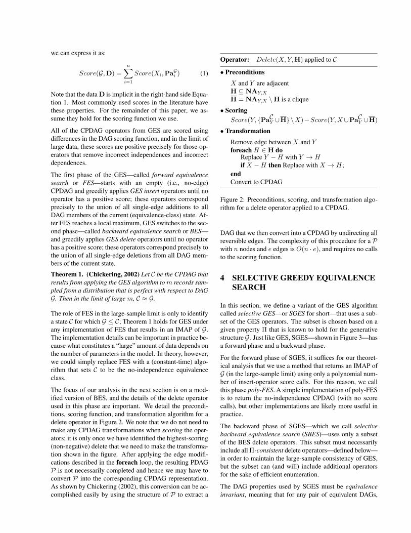
The focus of our analysis in the next section is on a mod-ified version of BES, and the details of the delete operatorused in this phase are important. We detail the precondi-tions, scoring function, and transformation algorithm for adelete operator in Figure 2. We note that we do not need tomake any CPDAG transformations when scoring the oper-ators; it is only once we have identified the highest-scoring(non-negative) delete that we need to make the transforma-tion shown in the figure. After applying the edge modifi-cations described in the foreach loop, the resulting PDAGP is not necessarily completed and hence we may have toconvert P into the corresponding CPDAG representation.As shown by Chickering (2002), this conversion can be ac-complished easily by using the structure of P to extract a

Operator: Delete(X,Y,H) applied to C

• Preconditions

X and Y are adjacentH ⊆ NAY,X

H = NAY,X \H is a clique

• ScoringScore(Y, {PaCY ∪H}\X)−Score(Y,X ∪PaCY ∪H)

• Transformation

Remove edge between X and Yforeach H ∈ H do

Replace Y −H with Y → Hif X −H then Replace with X → H;

endConvert to CPDAG

Figure 2: Preconditions, scoring, and transformation algo-rithm for a delete operator applied to a CPDAG.

DAG that we then convert into a CPDAG by undirecting allreversible edges. The complexity of this procedure for a Pwith n nodes and e edges is O(n · e), and requires no callsto the scoring function.

4 SELECTIVE GREEDY EQUIVALENCESEARCH

In this section, we define a variant of the GES algorithmcalled selective GES—or SGES for short—that uses a sub-set of the GES operators. The subset is chosen based on agiven property Π that is known to hold for the generativestructure G. Just like GES, SGES—shown in Figure 3—hasa forward phase and a backward phase.

For the forward phase of SGES, it suffices for our theoret-ical analysis that we use a method that returns an IMAP ofG (in the large-sample limit) using only a polynomial num-ber of insert-operator score calls. For this reason, we callthis phase poly-FES. A simple implementation of poly-FESis to return the no-independence CPDAG (with no scorecalls), but other implementations are likely more useful inpractice.

The backward phase of SGES—which we call selectivebackward equivalence search (SBES)—uses only a subsetof the BES delete operators. This subset must necessarilyinclude all Π-consistent delete operators—defined below—in order to maintain the large-sample consistency of GES,but the subset can (and will) include additional operatorsfor the sake of efficient enumeration.

The DAG properties used by SGES must be equivalenceinvariant, meaning that for any pair of equivalent DAGs,

either the property holds for both of them or it holds forneither of them. Thus, for any equivalence-invariant DAGproperty Π, it makes sense to say that Π either holds ordoes not hold for a PDAG. As shown by Chickering (1995),a DAG property is equivalence invariant if and only if it isinvariant to covered-edge reversals; it follows that the prop-erty that each node has at most k parents is equivalence in-variant, whereas the property that the length of the longestdirected path is at least k is not. Furthermore, the proper-ties for SGES must also be hereditary, which means thatif Π holds for a PDAG P it must also hold for all inducedsubgraphs of P . For example, the max-parent property ishereditary, whereas the property that each node has at leastk parents is not. We use EIH property to refer to a propertythat is equivalence invariant and hereditary.

Definition 1. Π-Consistent GES DeleteA GES delete operatorDelete(X,Y,H) is Π consistent forCPDAG C if, for the set of common descendants W of Xand Y in the resulting CPDAG C′, the property holds forthe induced subgraph C′[X ∪ Y ∪W].

In other words, after the delete, the property holds for thesubgraph defined byX , Y , and their common descendants.

Algorithm SGES(D,Π)

Input : Data D, Property ΠOutput: CPDAG CC ←− poly-FESC ←− SBES(D, C, Π)return C

Figure 3: Pseudo-code for the SGES algorithm.

Algorithm SBES(D, C,Π)

Input : Data D, CPDAG C, Property ΠOutput: CPDAG

RepeatOps←− Generate Π-consistent delete operators for COp←− highest-scoring operator in Opsif score of Op is negative then return CC ←− Apply Op to C

Figure 4: Pseudo-code for the SBES algorithm.

4.1 LARGE-SAMPLE CORRECTNESS

The following theorem establishes a graph-theoretic justi-fication for considering only the Π-consistent deletions ateach step of SBES.

Theorem 2. If G < C for CPDAG C and DAG G, thenfor any EIH property Π that holds on G, there exists a Π-

consistent Delete(X,Y,H) that when applied to C resultsin the CPDAG C′ for which G ≤ C′.

We postpone the proof of Theorem 2 to the appendix. Theresult is a consequence of an explicit characterization of,for a given pair of DAGs G and H such that G < H, anedge in H that we can either reverse or delete in H suchthat for the resulting DAGH′, we have G ≤ H′3.

Theorem 3. Let C be the CPDAG that results from apply-ing the SGES algorithm to (1) m records sampled from adistribution that is perfect with respect to DAG G and (2)EIH property Π that holds on G. Then in the limit of largem, C ≈ G.

Proof: Because the scoring function is locally consistent,we know poly-FES must return an IMAP of G. BecauseSBES includes all the Π-consistent delete operators, The-orem 2 guarantees that, unless C ≈ G, there will be apositive-scoring operator.

4.2 COMPLEXITY MEASURES

In this section, we discuss a number of distributional as-sumptions that we can use with Theorem 3 to limit the num-ber of operators that SGES needs to score. As discussed inSection 2, when we assume the generative distribution isperfect with respect to a DAG G, then graph-theoretic as-sumptions about G can lead to more efficient training algo-rithms. Common assumptions used include (1) a maximumparent-set size for any node, (2) a maximum-clique4 sizeamong any nodes and (3) a maximum treewidth. Treewidthis important because the complexity of exact inference isexponential in this measure.

We can associate a property with each of these assumptionsthat holds precisely when the DAG G satisfies that assump-tion. Consider the constraint that the maximum number ofparents for any node in G is some constant k. Then, us-ing “PS” to denote parent size, we can define the propertyΠk

PS to be true precisely for those DAGs in which eachnode has at most k parents. Similarly we can define Πk

CL

and ΠkTW to correspond to maximum-clique size and max-

imum treewidth, respectively.

For two properties Π and Π′, we write Π ⊆ Π′ if for everyDAG G for which Π holds, Π′ also holds. In other words,Π is a more constraining property than is Π′. Because thelowest node in any clique has all other nodes in the cliqueas parents, it is easy to see that Πk

PS ⊆ Πk−1CL . Because the

treewidth for DAG G is defined to be the size of the largestclique minus one in a graph whose cliques are at least aslarge as those in G, we also have Πk

TW ⊆ Πk−1CL . Which

3Chickering (2002) characterizes the reverse transformation ofreversals/additions in G, which provides an implicit characteriza-tion of reversals/deletions in H.

4We use clique in a DAG to mean a set of nodes in which allpairs are adjacent.

property to use will typically be a trade-off between howreasonable the assumption is (i.e, less constraining proper-ties are more reasonable) and the efficiency of the resultingalgorithm (i.e., more constraining properties lead to fasteralgorithms).

We now consider a new complexity measure called v-width,whose corresponding property is less constraining than theprevious three, and somewhat remarkably leads to an effi-cient implementation in SGES. For a DAG G, the v-widthis defined to be the maximum of, over all pairs of non-adjacent nodes X and Y , the size of the largest cliqueamong common children of X and Y . In other words,v-width is similar to the maximum-clique-size bound, ex-cept that the bound only applies to cliques of nodes that areshared children of some pair of non-adjacent nodes. Withthis understanding it is easy to see that, for the propertyΠk

VW corresponding to a bound on the v-width, we haveΠk

CL ⊆ ΠkVW .

To illustrate the difference between v-width and the othercomplexity measures, consider the two DAGs in Figure 5.The DAG in Figure 5(a) has a clique of size K, and con-sequently a maximum-clique size of K and a maximumparent-set size of K − 1. Thus, if K is O(n) for a largegraph of n nodes, any algorithm that is exponential in thesemeasures will not be efficient. The v-width, however, iszero for this DAG. The DAG in Figure 5(b), on the otherhand, has a v-width of K.

(a)

X1

A B

X2X3

X4

XKX1

A B

X2X3

X4

XK

(b)

Figure 5: Two DAGs (a) and (b) having identical maximumclique sizes, similar maximum number of parents, and di-vergent v-widths.

In order to use a property with SGES, we need to estab-lish that it is EIH. For Πk

PS , ΠkCL and Πk

VW , equivalence-invariance follows from the fact that all three properties arecovered-edge invariant, and hereditary follows because thecorresponding measures cannot increase when we removenodes and edges from a DAG. Although we can estab-lish EIH for the treewidth property Πk

TW with more work,we omit further consideration of treewidth for the sake ofspace.

4.3 GENERATING DELETIONS

In this section, we show how to generate a set of dele-tion operators for SBES such that all Π-consistent deletionoperators are included, for any Π ∈ {Πk

PS ,ΠkCL,Π

kVW }.

Furthermore, the total number of deletion operators wegenerate is polynomial in the number of nodes in the do-main and exponential in k.

Our approach is to restrict the Delete(X,Y,H) operatorsbased on the H sets and the resulting CPDAG C′. In par-ticular, we rule out candidate H sets for which Π doesnot hold on the induced subgraph C′[H ∪X ∪ Y ]; becauseall nodes in H will be common children of X and Y inC′—and thus a subset of the common descendants of Xand Y—we know from Definition 1 (and the fact that Π ishereditary) that none of the dropped operators can be Π-consistent.

Before presenting our restricted-enumeration algorithm,we now discuss how to enumerate delete operators with-out restrictions. As shown by Andersson et al. (1997), aCPDAG is a chain graph whose undirected components arechordal. This means that the induced sub-graph definedover NAY,X—which is a subset of the neighbors of Y—isan undirected chordal graph. A useful property of chordalgraphs is that we can identify, in polynomial time, a set ofmaximal cliques over these nodes5; let C1, ...,Cm denotethe nodes contained within these m maximal cliques, andlet H = NAY,X \ H be the complement of the sharedneighbors with respect to the candidate H. Recall fromFigure 2 that the preconditions for any Delete(X,Y,H)include the requirement that H is a clique. This means thatfor any valid H, there must be some maximal clique Ci thatcontains the entirety of H; thus, we can generate all oper-ators (without regard to any property) by stepping througheach maximal clique Ci in turn, initializing H to be allnodes not in Ci, and then generating a new operator cor-responding to expanding H by all subsets of nodes in Ci.Note that if NAY,X is itself a clique, we are enumeratingover all 2|NAY,X | operators.

As we show below, all three of the properties of interestimpose a bound on the maximum clique size among nodesin H. If we are given such a bound s, we know that any“expansion” subset for a clique that has size greater thans will result in an operator that is not valid. Thus, we canimplement the above operator-enumeration approach moreefficiently by only generating subsets within each cliquethat have size at most s. This allows us to process eachclique Ci with only O(|Ci + 1|s) calls to the scoring func-tion. In addition, we need not enumerate over any of thesubsets of Ci if, after removing this clique from the graph,there remains a clique of size greater than s; we define the

5Blair and Peyton (1993) provide a good survey on chordalgraphs and detail how to identify the maximal cliques while run-ning maximum-cardinality search.

Algorithm SELECTIVE-GENERATE-OPS(C, X, Y, s)

Input : CPDAG C with adjacent X ,Y and limit sOutput: Ops = {H1, . . . ,Hm}

Ops←− ∅Generate maximal cliques C1, ...,Cm from NAY,X

S←− FiltertCliques({C1, . . . ,Cm}, s)foreach Ci ∈ S do

H0 ←− NAY,X \Ci

foreach C ⊆ Ci with |C| ≤ s doAdd H0 ∪C to Ops

endendreturn Ops

Figure 6: Algorithm to generate clique-size limited deleteoperators.

function FilterCliques({C1, . . . ,Cm}, s) to be the sub-set of cliques that remain after imposing this constraint.With this function, we can define SELECTIVE-GENERATE-OPS as shown in Figure 6 to leverage the max-clique-sizeconstraint when generating operators; this algorithm will inturn be used to generate all of the CPDAG operators duringSBES.

Example: In Figure 7, we show an example CPDAG forwhich to run SELECTIVE-GENERATE-OPS(C, X , Y , s) forvarious values of s. In the example, there is a single cliqueC = {A,B} in the set NAY,X , and thus at the top of theouter foreach loop, the set H0 is initialized to the emptyset. If s = 0, the only subset of C with size zero is theempty set, and so that is added to Ops and the algorithmreturns. If s = 1 we add, in addition to the empty set, allsingleton subsets of C. For s ≥ 2, we add all subsets ofC.

Now we discuss how each of the three properties impose aconstraint s on the maximum clique among nodes in H, andconsequently the selective-generation algorithm in Figure 6can be used with each one, given an appropriate bound s.For both Πk

VW and ΠkCL, the k given imposes an explicit

bound on s (i.e., s = k for both). Because any clique inH of size r will result in a DAG member of the resultingequivalence class having a node in that clique with at leastr+ 1 parents (i.e., r− 1 from the other nodes in the clique,plus both X and Y ), we have for Πk

PS , s = k − 1.

We summarize the discussion above in the followingproposition.

Proposition 1. Algorithm SELECTIVE-GENERATE-OPSapplied to all edges using clique-size bound s gen-erates all Π-consistent delete operators for Π ∈{Πs+1

PS ,ΠsCL,Π

sVW }.

We now argue that running SBES on a domain of n vari-ables when using Algorithm SELECTIVE-GENERATE-OPSwith a bound s requires only a polynomial number in n ofcalls to the scoring function. Each clique in the inner loopof the algorithm can contain at most n nodes, and thereforewe generate and score at most (n+1)s operators, requiringat most 2(n + 1)s calls to the scoring function. Becausethe cliques are maximal, there can be at most n of themconsidered in the outer loop. Because there are never morethan n2 edges in a CPDAG, and we will delete at most allof them, we conclude that even if we decided to rescore ev-ery operator after every edge deletion, we will only make apolynomial number of calls to the scoring function.

From the above discussion and the fact that SBES com-pletes using at most a polynomial number of calls to thescoring function, we get the following result for the fullSGES algorithm.

Proposition 2. The SGES algorithm, when run over a do-main of n variables and given Π ∈ {Πs+1

PS ,ΠsCL,Π

sVW },

runs to completion using a number of calls to the DAGscoring function that is polynomial in n and exponentialin s.

A B

X Ys=0 Ops={ {} }s=1 Ops={ {}, {A}, {B} }s=2 Ops={ {} ,{A}, {B}, {A,B} }

Figure 7: An example CPDAG C and the resulting opera-tors generated by SELECTIVE-GENERATE-OPS(C,X ,Y ,s)for various values of s.

5 EXPERIMENTS

In this section, we present a simple synthetic experimentcomparing SBES and BES that demonstrates the value ofpruning operators. In our experiment we used an oraclescoring function. In particular, given a generative model G,our scoring function computes the minimum-description-length score assuming a data size of five billion records,but without actually sampling any data: instead, we useexact inference in G (i.e., instead of counting from data)to compute the conditional probabilities needed to computethe expected log loss. This allows us to get near-asymptoticbehavior without the need to sample data. To evaluate thecost of running each algorithm, we counted the number oftimes the scoring function was called on a unique node andparent-set combination; we cached these scores away sothat if they were needed multiple times during a run of thealgorithm, they were only computed (and counted) once.

In Figure 8, we show the average number of scoring-function calls required to complete BES and SBES whenstarting from a complete graph over a domain of n bi-nary variables, for varying values of n. Each average istaken over ten trials, corresponding to ten random genera-tive models. All variables in the domain were binary. Wegenerated the structure of each generative model as follows.First, we enumerated all node pairs by randomly permutingthe nodes and taking each node in turn with all of its pre-decessors in turn. For each node pair in turn, we chose toattempt an edge insertion with probability one half. Foreach attempt, we added an edge if doing so (1) did not cre-ate a cycle and (2) did not result in a node having morethan two parents; if an edge could be added in either di-rection, we chose the direction at random. We sampledthe conditional distributions for each node and each par-ent configuration from a uniform Dirichlet distribution withequivalent-sample size of one. We ran SBES with Π2

PS .

0

5000

10000

15000

20000

25000

5 6 7 8 9 10 11 12

Sco

re E

vlau

atio

ns

Number of Nodes

BES

SBES

Figure 8: Number of score evaluations needed to run BESand SBES, starting from the complete graph, for a range ofdomain sizes.

Our results show clearly the exponential dependence ofBES on the number of nodes in the clique, and the increas-ing savings we get with SBES, leveraging the fact that Π2

PS

holds in the generative structure.

Note that to realize large savings in practice, when GESruns FES instead of starting from a dense graph, a (rel-atively sparse) generative distribution must lead FES to anequivalence class containing a (relatively dense) undirectedclique that is subsequently “thinned” during BES. We cansynthesize challenging grid distributions to force FES intosuch states, but it is not clear how realistic such distribu-tions are in practice. When we re-run the clique experi-ment above, but where we instead start both BES and SBESfrom the model that results from running FES (i.e., withno polynomial-time guarantee), the savings from SBES are

small due to the fact that the subsequent equivalence classesdo not contain large cliques.

6 CONCLUSION

Through our selective greedy equivalence search algo-rithm SGES, we have demonstrated how to leveragegraph-theoretic properties to reduce the need to scoregraphs during score-based search over equivalence classesof Bayesian networks. Furthermore, we have shownthat for graph-theoretic complexity properties includingmaximum-clique size, maximum number of parents, andv-width, we can guarantee that the number of score evalua-tions is polynomial in the number of nodes and exponentialin these complexity measures.

The fact that we can use our approach to selectivelychoose operators for any hereditary and equivalence in-variant graph-theoretic property provides the opportunityto explore alternative complexity measures. Another can-didate complexity measure is the maximum number of v-structures. Although the corresponding property does notlimit the maximum size of a clique in H, it limits directlythe size |H| for every operator. Thus it would be easy toenumerate these operators efficiently. Another complexitymeasure of interest is treewidth, due to the fact that exactinference in a Bayesian-network model is takes time expo-nential in this measure.

The results we have presented are for the general Bayesian-network learning problem. It is interesting to consider theimplications of our results for the problem of learning par-ticular subsets of Bayesian networks. One natural class thatwe discussed in Section 2 is that of polytrees. If we assumethat the generative distribution is perfect with respect to apolytree then we know the v-width of the generative graphis one. This implies, in the limit of large data, that we canrecover the structure of the generative graph with a poly-nomial number of score evaluations. This provides a score-based recovery algorithm analogous to the constraint-basedapproach of Geiger et al. (1990).

We presented a simple complexity analysis for the purposeof demonstrating that SGES uses a only polynomial num-ber of calls to the scoring function. We leave as future worka more careful analysis that establishes useful constants inthis polynomial. In particular, we can derive tighter boundson the total number of node-and-parent-configurations thatare needed to score all the operators for each CPDAG, andby caching these configuration scores we can further takeadvantage of the fact that most operators remain valid (i.e.,the preconditions still hold) and have the same score aftereach transformation.

Finally, we plan to investigate practical implementations ofpoly-FES that have the polynomial-time guarantees neededfor SGES.

Appendices

In the following two appendices, we prove Theorem 2.

A Additional Background

In this section, we introduce additional background mate-rial needed for the proofs.

A.1 Additional Notation

To express sets of variables more compactly, we often usea comma to denote set union (e.g., we write X = Y,Z as amore compact version of X = Y ∪Z). We also will some-times remove the comma (e.g., YZ). When a set consistsof a singleton variable, we often use the variable name asshorthand for the set containing that variable (e.g., we writeX = Y \ Z as shorthand for X = Y \ {Z}).

We say a nodeN is a descendant of Y ifN = Y or there isa directed path from Y toN . We useH-descendant to referto a descendant in a particular DAG H. We say a node Nis a proper descendant of Y if N is a descendant of Y andN 6= Y . We use NonDeHY to denote the non-descendantsof node Y in G. We use PaHY ↓X1X2...Xn

as shorthand forPaHY \ {X1, . . . , Xn}. For example, to denote all the par-ents of Z inH except for X and Y , we use PaHZ↓XY .

A.2 D-separation and Acvite Paths

The independence constraints implied by a DAG structureare characterized by the d-separation criterion. Two nodesA and B are said to be d-separated in a DAG G given aset of nodes S if and only if there is no active path in Gbetween A and B given S. The standard definition of anactive path is a simple path for which each node W alongthe path either (1) has converging arrows (i.e., → W ←)and W or a descendant of W is in S or (2) does not haveconverging arrows and W is not in S. By simple, we meanthat the path never passes through the same node twice.

To simplify our proofs, we use an equivalent definition ofan active path—that need not be simple—where each nodeW along the path either (1) has converging arrows andW isin S or (2) does not have converging arrows andW is not inS. In other words, instead of allowing a segment→ W ←to be included in a path by virtue of a descendant of W be-longing to S, we require that the path include the sequenceof edges from W to that descendant and then back again.For those readers familiar with the celebrated “Bayes ball”algorithm of Shachter (1998) for testing d-separation, ourexpanded definition of an active path is simply a valid paththat the ball can take between A and B.

We use X⊥⊥GY|Z to denote the assertion that DAG G im-poses the constraint that variables X are independent ofvariables Y given variables Z.When a nodeW along a path

has converging arrows, we say that W is a collider at thatposition in the path.

The direction of each terminal edge in an active path—thatis, the first and last edge encountered in a traversal from oneend of the path to the other—is important for determiningwhether we can append two active paths together to makea third active path. We say that a path π(A,B) is into A ifthe terminal edge incident to A is oriented toward A (i.e.,A ←). Similarly, the path is into B if the terminal edgeincident to B is oriented toward B. If a path is not intoan endpoint A, we say that the path is out of A. Using thefollowing result from Chickering (2002), we can combineactive paths together.

Lemma 1. (Chickering, 2002) Let π(A,B) be an S-activepath between A and B, and let π(B,C) be an S-activepath between B and C. If either path is out of B, then theconcatenation of π(A,B) and π(B,C) is an S-active pathbetween A and C.

Given a DAG H that is an IMAP of DAG G, we use thed-separation criterion in two general ways in our proofs.First, we identify d-separation facts that hold inH and con-clude that they must also hold in G. Second, we identifyactive paths in G and conclude that there must be corre-sponding active paths inH.

A.3 Independence Axioms

In many of our proofs, we would like to reason about theindependence facts that hold in DAG G without knowingwhat its structure is, which makes using the d-separationcriterion problematic. As described in Pearl (1988), anyset of independence facts characterized by the d-separationcriterion also respect the independence axioms shown inFigure 9. These axioms allow us to take a set of indepen-dence facts in some unknown G (e.g., that are implied byd-separation inH), and derive new independence facts thatwe know must also hold in G.

Throughout the proofs, we will often use the Symmetryaxiom implicitly. For example, if we have A⊥⊥B,C|D wemight claim that B⊥⊥A|C,D follows from Weak Union,as opposed to concluding A⊥⊥B|C,D from Weak Unionand then applying Symmetry. We will frequently identifyindependence constraints in H and conclude that theyhold in G, without explicitly justifying this with becauseG ≤ H. For example, we will say:

Because A is a non-descendant of B in H, it follows fromthe Markov conditions that A⊥⊥GB|PaHB .

In other words, to be explicit we would say thatA⊥⊥HB|PaHB follows from the Markov conditions, andthe independence holds in G because G ≤ H.

Symmetry: X⊥⊥Y|Z ⇐⇒ Y⊥⊥X|ZDecomposition: X⊥⊥Y,W|Z =⇒ X⊥⊥Y|Z + X⊥⊥W|ZComposition: X⊥⊥Y|Z + X⊥⊥W|Z =⇒ X⊥⊥Y,W|ZIntersection: X⊥⊥Y|Z,W + X⊥⊥W|Z,Y =⇒ X⊥⊥Y,W|ZWeak Union: X⊥⊥Y,W|Z =⇒ X⊥⊥Y|Z,WContraction: X⊥⊥W|Z,Y + X⊥⊥Y|Z ⇐= X⊥⊥Y,W|ZWeak Transitivity: X⊥⊥Y|Z + X⊥⊥Y|Z, T =⇒ X⊥⊥T |Z OR Y⊥⊥T |Z

Figure 9: The DAG-perfect independence axioms.

The Composition axiom states that if X is independent ofboth Y and W individually given Z, then X is independentof them jointly. If we have more than two such sets that areindependent of X, we can apply the Composition axiom re-peatedly to combine them all together. To simplify, we willdo this combination implicitly, and assume that the Compo-sition axiom is defined more generally. Thus, for example,we might have:

Because X⊥⊥Y |Z for every Y ∈ Y, we conclude by theComposition axiom that X⊥⊥Y|Z.

B Proofs

In this section, we provide a number of intermediate resultsthat lead to a proof of Theorem 2.

B.1 Intermediate Result: “The Deletion Lemma”

Given DAGs G and H for which G < H, we say that anedge e from H is deletable in H with respect to G if, forthe DAGH′ that results after removing e fromH, we haveG ≤ H. We will say that an edge is deletable in H orsimply deletable if G or both DAGs, respectively, are clearfrom context. The following lemma establishes necessaryand sufficient conditions for an edge to be deletable.Lemma 2. Let G and H be two DAGs such that G ≤ H.An edge X → Y is deletable in H with respect to G if andonly if Y⊥⊥GX|PaHY \X .

Proof: Let H′ be the DAG resulting from removing theedge. The “only if” follows immediately because the givenindependence is implied by H′. For the “if”, we show thatfor every nodeA and every nodeB ∈ NonDeH

′

A , the inde-pendence A⊥⊥GB|PaH

′

A holds (in G). We need only con-sider (A,B) pairs for whichB is a descendant inH but notinH′; if the “descendant” relationship has not changed, weknow the independence holds by virtue of G ≤ H and thefact that deleting an edge results in strictly more indepen-dence constraints.

The proof follows by induction on the length of the longestdirected path in H′ from Y to B. For the base case (seeFigure 10a and Figure 10b), we start with a longest pathof length zero; in other words, B = Y . Because A is an

ancestor of Y in H, both it and its parents must be non-descendants of Y in H, and therefore the Markov condi-tions inH imply

Y⊥⊥GA,PaHA |PaHY (2)

Given the independence fact assumed in the lemma, we canapply the Contraction axiom to remove X from the condi-tioning set in (2), and then apply the Weak Union axiom tomove PaHA into the conditioning set to conclude

Y⊥⊥GA|PaHY \X,PaHA (3)

Neither Y nor its new parents PaHY \X can be descendantsofA inH′, elseB would remain a descendant ofA after thedeletion, and thus we conclude by the Markov conditionsinH that

A⊥⊥GPaHY \X|PaHA (4)

Applying the Contraction axiom to (3) and (4), we have

A⊥⊥GY |PaHA

and because PaH′

A = PaHA the lemma follows.

For the induction step (see Figure 10c and Figure 10d), weassume the lemma holds for all nodes whose longest pathfrom Y is ≤ k, and we consider a B for which the longestpath from Y is k + 1. Consider any parent P of node B.If P is a descendant of Y , the longest path from Y to Bmust be ≤ k, else we have a path to B that is longer thank + 1. If P is not a descendant of Y , then P is also not adescendant of A in H, else B would be a descendant of AinH′. Thus, for every parent P , we conclude

A⊥⊥GP |PaHA

either by the induction hypothesis or by the fact that P is anon-descendant of A in H. From the Composition axiomwe can combine these individual parents together, yielding

A⊥⊥GPaHB |PaHA (5)

Because B is a descendant of A inH, we know that A andall of its parents PaHA are non-descendants of B in H, andthus

B⊥⊥GA,PaHA |PaHB (6)

(c)

(d)

X

Y

P1 Pn

B

k+1

A

PaA

X

Y

P1 Pn

B

A

PaA

X

Y=B

PaY X

A

PaA

X

Y=B

PaY X

A

PaA

(a)

(b)

PaB PaB

Figure 10: Relevant portions ofH andH′ for the inductive proof of Lemma 2: (a) and (b) are for the basis and (c) and (d)are for the induction hypothesis.

Applying the Weak Union axiom to (6) yields

B⊥⊥GA|PaHA ,PaHB (7)

and finally applying the Contraction axiom to (5) and (7)yields

A⊥⊥GB|PaHA

Because the parents of A are the same in both H and H′,the lemma follows.

B.2 Intermediate Result: “The Deletion Theorem”

We define the pruned variables for G and H—denotedPrune(G,H)– to be the subset of the variables that remainafter we repeatedly remove from both graphs any commonsink nodes (i.e., nodes with no children) with the same par-ents in both graphs. For V = Prune(G,H), let V de-note the complement of V. Note that every node in V hasthe same parents and children in both G and H, and thatG[V] = H[V].

We use G-leaf to denote any node in G that has no children.For any G-leaf L, we say that L is anH-lowest G-leaf if noproper descendant of L in H is a G-leaf . Note that we arediscussing two DAGs in this case: L is a leaf in G, and outof all nodes that are leaves in G, L is the one that is lowestin the other DAG H. To avoid ambiguity, we often prefixother common graph concepts (e.g., G-child andH-parent)to emphasize the specific DAG to which we are referring.

We need the following result from Chickering (2002).

Lemma 3. (Chickering, 2002) Let G andH be two DAGscontaining a node Y that is a sink in both DAGs and forwhich PaGY = PaHY . Let G′ and H′ denote the subgraphsof G and H, respectively, that result by removing node Yand all its in-coming edges. Then G ≤ H if and only ifG′ ≤ H′.

By repeatedly applying Lemma 3, the following corollaryfollows immediately.

Corollary 1. Let V = Prune(G,H). Then G ≤ H if andonly if GV ≤ HV.

We now present the “deletion theorem”, which is the basisfor Theorem 2.

Theorem 4. Let G and H be DAGs for which G ≤ H, letV = Prune(G,H), and let L be any H[V]-lowest G[V]-leaf. Then,

1. If L does not have any H[V]-children, then for everyD ∈ V that is an H[V]-parent of L but not a G[V]-parent of L, D → L is deletable inH.

2. If L has at least one H[V]-child, let A be any H[V]-highest child; one of the following three propertiesmust hold inH:

(a) L→ A is covered.

(b) There exists an edge A← B, where L and B arenot adjacent, and either L → A or A ← B (orboth) are deletable.

(c) There exists an edgeD → L, whereD andA arenot adjacent, and either D → L or L → A (orboth) are deletable.

Proof: As a consequence of Corollary 1, the lemma holdsif and only if it holds for any graphs G and H for whichthere are no nodes that are sinks in both graphs with thesame parents; in other words, G = GV and H = HV.Thus, to vastly simplify the notation for the remainder ofthe proof, we will assume that this is the case, and thereforeL is a leaf node in G, A is a highest child of L in H, andthe restriction of B and D to V is vacuous.

For case (1), we know that PaGL ⊆ PaHL , else there wouldbe some edge in X → L in G for which X and L are notadjacent in H, contradicting G ≤ H. Because L is a leafin G, all non-parents must also be non-descendants, andhence L⊥⊥GX|PaGL for all X . It follows that for everyD ∈ {PaHL \PaGL}, D → Y is deletable inH. There mustexist such a D, else L would be in V = Prune(G,H).

For case (2), we now show that at least one of the propertiesmust hold. Assume that the first property does not hold,and demonstrate that one of the other two properties musthold. If the first property does not hold then we know thatin H either there exists an edge A ← B where B is not aparent of L, or there exists an edge D → L where D is nota parent of A. Thus the pre-conditions of at least one of theremaining two properties must hold.

SupposeH contains the edgeA← B whereB is not a par-ent of L. Then we conclude immediately from Corollary 2that either L→ A or A← B is deletable inH.

SupposeH contains the edgeD → L whereD is not a par-ent of A. Then the set D containing all parents of L thatare not parents of A is non-empty. Let R = PaHA ∩ PaHLbe the shared parents of L and A, and let T = PaH

A↓RL

be the remaining non-L parents of A inH, so that we havePaHA = L,R,T and PaHL = R,D. Because no node inD is a child or a descendant of A, lest H contains a cy-cle, we know that H contains the following independenceconstraint that must hold in G:

A⊥⊥GD|L,R,T (8)

Because L is a leaf node in G, it is impossible to create anew active path by removing it from the conditioning set,and hence we also know

A⊥⊥GD|R,T (9)

Applying the Weak Transitivity axiom to Independence 8and Independence 9, we conclude either A⊥⊥GL|R,T—in which case L→ A is deletable–or

L⊥⊥GD|R,T (10)

We know that no node in T can be a descendant of L, orelse A would not be the highest child of L. Thus, becauseL is independent of any non-descendants given its parentswe have

L⊥⊥GT|R,D (11)

Applying the Intersection axiom to Independence 10 andIndependence 11, we have

L⊥⊥GD|R (12)

In other words, L is independent of all of the nodes in Dgiven the other parents. By applying the Weak Union ax-iom, we can pull all but one of the nodes in D into theconditioning set to obtain

L⊥⊥GD|R, {D \D} (13)

and hence D → L is deletable for each such D.

B.3 Intermediate Result: “Add A SingletonDescendant to the Conditioning Set”

The intuition behind the following lemma is that if L isan H-lowest G-leaf , no v-structure below L in H can be“real” in terms of the dependences in G: for any Y below Lthat is independent of some other node X , they remain in-dependent when we condition on any singleton descendantZ of Y , even if Z is also a descendant of X . The lemmais stated in a somewhat complicated manner because wewant to use it both when (1) X and Y are adjacent but theedge is known to be deletable and (2) X and Y are not ad-jacent. We also find it convenient to include, in additionto Y ’s non-X parents, an arbitrary additional set of non-descendants S.

Lemma 4. Let Y be any H-descendant of an H-lowestG-leaf . If

Y⊥⊥GX|PaHY ↓X ,S

for {X,S} ⊆ NonDeHY , then Y⊥⊥GX|PaHY ↓X ,S, Z forany properH-descendant Z of Y .

Proof: To simplify notation, let R = PaHY ↓X ,S. Assumethe lemma does not hold and thus Y 6⊥⊥GX|R, Z. Considerany (R, Z)-active path πXY between X and Y in G. Be-cause Y⊥⊥GX|R, this path cannot be active without Z inthe conditioning set, which means that Z must be on thepath, and it must be a collider in every position it occurs.Without loss of generality, assumeZ occurs exactly once asa collider along the path (we can simply delete the sub-pathbetween the first and last occurrence of Z, and the resultingpath will remain active), and let πXZ be the sub-path fromX to Z along πXY , and let πZY be the sub-path from Z toY along πXY .

Because Z is a proper descendant of Y in H, and Y is adescendant of an H-lowest G-leaf , we know Z cannot bea G-leaf , else it would be lower than L in H. That means

that in G, there is a directed path πZL′ = Z → . . . → L′

consisting of at least one edge from Z to some G-leaf . Nonode T along this path can be in R, else we could splicein the path Z → . . . → T ← . . . ← Z between πXZ

and πZY , and the resulting path would remain active with-out Z in the conditioning set. Note that this means that L′

cannot belong to PaHY ↓X ⊆ R. Similarly, the path cannotreach X or Y , else we could combine this out-of-Z pathwith πZY or πXZ , respectively, to again find an R-activepath between X and Y . We know that in H, L′ must bea non-descendant of Y , else L′ would be a lower G-leafthan L in H. Because X ∪ R contains all of Y ’s parentsand none of its descendants, and because (as we noted) L′

cannot be inX∪R, we knowH contains the independenceY⊥⊥HL′|X,R. But we just argued that the (directed) pathπZL′ in G does not pass through any of X,Y,R, whichmeans that it constitutes an out-of Z (R, X)-active paththat can be combined with πZY to produce a (R, X)-activepath between Z and L′, yielding a contradiction.

B.4 Intermediate Result: The “Weak-TransitivityDeletion” Lemma

The next lemma considers a collider X → Z ← Y inH where either there is no edge between X and Y (i.e.,the collider is a v-structure) or the edge is deletable. Thelemma states that if X and Y remain independent whenconditioning on their common child—where all the non-{X,Y, Z} parents of all three nodes are also in the condi-tioning set—then one of the two edges must be deletable.

Lemma 5. Let X → Z and Y → Z be twoedges in H. If X⊥⊥GY |PaHX↓Y ,PaHY ↓X ,PaHZ↓XY andX⊥⊥GY |PaHX↓Y ,PaHY ↓X ,PaHZ↓XY , Z (i.e., Z added tothe conditioning set), then at least one of the following musthold: Z⊥⊥GX|PaHZ↓X or Z⊥⊥GY |PaHZ↓Y .

Proof: Let S = {PaHX↓Y ,PaHY ↓X}\PaHZ↓XY be the (non-X and non-Y ) parents of X and Y that are not parents ofZ, and let R = PaHZ↓XY be all of Z’s parents other thanX and Y . Using this notation, we can re-write the twoconditions of the lemma as:

X⊥⊥GY |R,S (14)

andX⊥⊥GY |Z,R,S (15)

From the Weak Transitivity axiom we conclude fromthese two independences that either Z⊥⊥GX|R,S orZ⊥⊥GX|R,S. Assume the first of these is true

Z⊥⊥GX|R,S (16)

If we apply the Composition axiom to the independencesin Equation 14 and Equation 16 we get X⊥⊥HY,Z|R,S;applying the Weak Union axiom we can then pull Y into

the conditioning set to get:

Z⊥⊥HX|{Y,R},S (17)

Because {Y,R}, X is precisely the parent set of Z, andbecause S (i.e., the parents of Z’s parents) cannot containany descendant of Z, we know by the Markov conditionsthat

Z⊥⊥HS|{Y,R}, X (18)

Applying the Intersection Axiom to the independences inEquation 17 and Equation 18 yields:

Z⊥⊥HX|Y,R

Because Y,R = PaHZ↓X , this means the first independenceimplied by the lemma follows.

If the second of the two independence facts that followfrom Weak Transitivity hold (i.e., if Z⊥⊥GX|R,S), then acompletely parallel application of axioms leads to the sec-ond independence implied by the lemma.

B.5 Intermediate Result: The “Move Lower” Lemma

Lemma 6. Let Y be any H-descendant of an H-lowestG-leaf . If there exists an X ∈ NonDeHY that has a com-monH-descendant with Y and for which

Y⊥⊥GX|PaHY ↓X

then there exists an edge W → Z that is deletable in H,where Z is a properH-descendant of Y .

Proof: Let Z be the highest common descendant of Y andX , let DY be the lowest descendant of Y that is a parentof Z, and let DX be any descendant of X that is a parentof Z. We know that either (1) DY = Y and DX = X or(2) DY and DX are not adjacent and have no directed pathconnecting them; if this were not the case, andH containeda path DY → . . . → DX (DX → . . . → DY ) then DX

(DY ) would be a higher common descendant than Z. Thismeans that in either case (1) or in case (2), we have

DY⊥⊥GDX |PaHDY ↓DX(19)

For case (1), this is given to us explicitly in the statementof the lemma, and for case (2), PaHDY ↓DX

= PaHDYand

thus the independence holds from the Markov conditionsin H because DX is a non-descendant of DY . Because inboth cases we know there is no directed path from DY toDX , we know that all of PaHDX↓DY

are non-descendants ofDY , and thus we can add them (via Composition and WeakUnion) to the conditioning set of Equation 19:

DY⊥⊥GDX |PaHDY ↓DX,PaHDX↓DY

(20)

For any PZ ∈ PaHZ↓DY DX(i.e., any parent of Z excluding

DY and DX ), we know that PZ cannot be a descendant of

DY , else PZ would have been chosen instead of DY as thelowest descendant of Y that is a parent of Z. Thus, we canyet again add to the conditioning set (via Composition andWeak Union) to get:

DY⊥⊥GDX |PaHDY ↓DX,PaHDX↓DY

,PaHZ↓DY DX(21)

Because no member of the conditioning set in Equation 21is a descendant of DY , and because DY , by virtue of beinga descendant of Y , must also be a descendant of the H-lowest G-leaf , we conclude from Lemma 4 that for (properH-descendant of Y ) Z we have:

DY⊥⊥GDX |PaHDY ↓DX,PaHDX↓DY

,PaHZ↓DY DX, Z

(22)Given Equation 21 and Equation 22, we can apply Lemma5 and conclude either (1) Z⊥⊥GDY |PaHZ↓DY

and henceDY → Z is deletable in H or (2) Z⊥⊥GDX |PaHZ↓DX

andhence DX → Z is deletable inHCorollary 2. Let L be an H-lowest G-leaf , and let A beanyH-highest child of L. If there exists an edge A← B inH for which L and B are not adjacent, then either L→ Aor A← B is deletable inH.

Proof: Because L is equal to (and thus a descendant of)an H-lowest G-leaf , it satisfies the requirement for “Y ” inthe statement of Lemma 6. Because A is the highest childof L, B cannot be a descendant of L and thus satisfies therequirement of “X” in the statement of Lemma 6. Fromthe proof of the lemma, if we choose A to be the highest-common descendant (i.e., “Z”), the corollary follows bynoting that because A is the highest H-child of L, L mustbe a lowest parent of A, and thus we can choose DY = LDX = B.

B.6 Intermediate Result: “The Move-DownCorollary”

Corollary 3. Let X → Y be any deletable edge within Hfor which Y is a descendant of an H-lowest G-leaf . Thenthere exists an edge Z → W that is deletable in H forwhich Z and W have no common descendants.

Proof: If X and Y have a common descendant, we knowfrom Lemma 6 that there must be another deletable edgeZ → W for which W is a proper descendant of Y , andthus Z and W satisfy the conditions for “X” and “Y ”, re-spectively, in the statement of Lemma 6, but with a lower“Y ” than we had before. Because H is acyclic, if we re-peatedly apply this argument we must reach some edge forwhich the endpoints have no common descendants.

B.7 Main Result: Proof of Theorem 2

Theorem 2 If G < C for CPDAG C and DAG G, thenfor any EIH property Π that holds on G, there exists a Π-consistent Delete(X,Y,H) that when applied to C resultsin the CPDAG C′ for which G ≤ C′.

Proof: Consider any DAG H0 in [C]≈. From Theorem 4,we know that there exists either a covered edge or deletableedge inH0; if we reverse any covered edge in DAGHi, theresulting DAG Hi+1 (which is equivalent to Hi) will becloser to G in terms of total edge differences, and thereforebecause H0 6= G we must eventually reach an H = Hi forwhich Theorem 4 identifies a deletable edge e. The edge einH satisfies the preconditions of Corollary 3, and thus weknow that there must also exist a deletable edge X → Yin H for which X and Y have no common descendants inH[V] for V = Prune(G,H).

Let H′ be the DAG that results from deleting the edgeX → Y in H. Because there is a GES delete opera-tor corresponding to every edge deletion in every DAGin [C]≈, we know there must be a set H for which theoperator Delete(X,Y,H)—when applied to C—results inC′ = [H′]≈. Because X → Y is deletable in H, the op-erator satisfies the IMAP requirement in the theorem. Forthe remainder of the proof, we demonstrate that it is Π-consistent.

Because all directed edges in C′ are compelled, these edgesmust exist with the same orientation in all DAGs in [C′]≈;it follows that any subset W of the common descendantsof X and Y in C′ must also be common descendants ofX and Y in H′. But because X and Y have no commondescendants in the “pruned” subgraphH[V], we know thatW is contained entirely in the complement of V, whichmeansH[W] = G[W]; becauseH′ is the same asH exceptfor the edge X → Y , we concludeH′[W] = G[W].

We now consider the induced subgraph H′[W ∪X ∪ Y ]that we get by “expanding” the graph H′[W] to include Xand Y . Because X and Y are not adjacent in H′, and be-causeH′ is acyclic, any edge inH′[W ∪X ∪ Y ] that is notinH′[W] must be directed from either X or Y into a nodein the descendant set W. Because all nodes in W are inthe complement of V, these new edges must also exist inG, and we conclude H′[W ∪X ∪ Y ] = G[W ∪X ∪ Y ].To complete the proof, we note that because Π is heredi-tary, it must hold on H′[W ∪X ∪ Y ]. From Proposition??, we know H′[W ∪X ∪ Y ] ≈ C′[W ∪X ∪ Y ]), andtherefore because Π is equivalence invariant, it holds forC′[W ∪X ∪ Y ].

References

[1] Pieter Abbeel, Daphne Koller, and Andrew Y. Ng.Learning factor graphs in polynomial time and samplecomplexity. Journal of Machine Learning Research,7:1743–1788, 2006.

[2] Steen A. Andersson, David Madigan, and Michael D.Perlman. A characterization of Markov equivalenceclasses for acyclic digraphs. Annals of Statistics,25:505–541, 1997.

[3] Jean R. S. Blair and Barry W. Peyton. An introductionto chordal graphs and clique trees. In Graph Theoryand Sparse Matrix Computations, pages 1–29, 1993.

[4] David Maxwell Chickering. A transformational char-acterization of Bayesian network structures. InS. Hanks and P. Besnard, editors, Proceedings ofthe Eleventh Conference on Uncertainty in ArtificialIntelligence, Montreal, QU, pages 87–98. MorganKaufmann, August 1995.

[5] David Maxwell Chickering. Learning Bayesian net-works is NP-Complete. In D. Fisher and H.J. Lenz,editors, Learning from Data: Artificial Intelligenceand Statistics V, pages 121–130. Springer-Verlag,1996.

[6] David Maxwell Chickering. Optimal structure iden-tification with greedy search. Journal of MachineLearning Research, 3:507–554, November 2002.

[7] David Maxwell Chickering and Christopher Meek.Finding optimal Bayesian networks. In A. Darwicheand N. Friedman, editors, Proceedings of the Eigh-teenth Conference on Uncertainty in Artificial Intelli-gence, Edmonton, AB, pages 94–102. Morgan Kauf-mann, August 2002.

[8] David Maxwell Chickering and Christopher Meek.Selective greedy equivalence search: Finding opti-mal Bayesian networks using a polynomial number ofscore evaluations. In Proceedings of the Thirty FirstConference on Uncertainty in Artificial Intelligence,Amsterdam, Netherlands, 2015.

[9] David Maxwell Chickering and Christopher Meek.Selective greedy equivalence search: Finding opti-mal Bayesian networks using a polynomial numberof score evaluations. 2015, arxiv:1506.2849v1.

[10] David Maxwell Chickering, Christopher Meek, andDavid Heckerman. Large-sample learning ofBayesian networks is NP-hard. Journal of MachineLearning Research, 5:1287–1330, October 2004.

[11] C. Chow and C. Liu. Approximating discrete prob-ability distributions with dependence trees. IEEETransactions on Information Theory, 14:462–467,1968.

[12] S. Dasgupta. Learning polytrees. In K. Laskeyand H. Prade, editors, Proceedings of the FifteenthConference on Uncertainty in Artificial Intelligence,Stockholm, Sweden, pages 131–141. Morgan Kauf-mann, 1999.

[13] J. Edmonds. Optimum branching. J. Res. NBS,71B:233–240, 1967.

[14] Nir Friedman, Iftach Nachman, and Dana Peer.Learning bayesian network structure from massivedatasets: The “sparse candidate” algorithm. In Pro-ceedings of the Fifteenth Conference on Uncertaintyin Artificial Intelligence, Stockholm, Sweden. Mor-gan Kaufmann, 1999.

[15] Serge Gaspers, Mikko Koivisto, Mathieu Liedloff,Sebastian Ordyniak, and Stefan Szeider. On findingoptimal polytrees. In Proceedings of the Twenty-SixthAAAI Conference on Artificial Intelligence. AAAIPress, 2012.

[16] Dan Geiger, Azaria Paz, and Judea Pearl. Learningcausal trees from dependence information. In Pro-ceedings of the Eighth National Conference on Arti-ficial Intelligence - Volume 2, AAAI’90, pages 770–776. AAAI Press, 1990.

[17] Steven B. Gillispie and Michael D. Perlman. Enumer-ating Markov equivalence classes of acyclic digraphmodels. In M. Goldszmidt, J. Breese, and D. Koller,editors, Proceedings of the Seventeenth Conferenceon Uncertainty in Artificial Intelligence, Seattle, WA,pages 171–177. Morgan Kaufmann, 2001.

[18] Markus Kalisch and Peter Buhlmann. Estimatinghigh-dimensional directed acyclic graphs with the pcalgorithm. Journal of Machine Learning Research,8:613–636, 2007.

[19] David Karger and Nathan Srebro. Learning Markovnetworks: Maximum bounded tree-width graphs. In12th ACM-SIAM Symposium on Discrete Algorithms(SODA), pages 391–401, January 2001.

[20] Mikko Koivisto and Kismat Sood. Exact bayesianstructure discovery in bayesian networks. J. Mach.Learn. Res., 5:549–573, December 2004.

[21] Kaname Kojima, Eric Perrier, Seiya Imoto, andSatoru Miyano. Optimal search on clustered struc-tural constraint for learning Bayesian network struc-ture. Journal of Machine Learning Resarch, 11:285–310, 2010.

[22] Christopher Meek. Finding a path is harder than find-ing a tree. Journal of Artificial Intelligence Research,15:383–389, 2001.

[23] Mukund Narasimhan and Jeff Bilmes. Pac-learningbounded tree-width graphical models. In Proceed-ings of the 20th Conference on Uncertainty in Artifi-cial Intelligence, UAI ’04, pages 410–417, Arlington,Virginia, United States, 2004. AUAI Press.

[24] Sebastian Ordyniak and Stefan Szeider. Parameter-ized complexity results for exact bayesian networkstructure learning. Journal of Artificial IntelligenceResearch, 46:263–302, 2013.

[25] Judea Pearl. Probabilistic Reasoning in IntelligentSystems: Networks of Plausible Inference. MorganKaufmann, San Mateo, CA, 1988.

[26] Dafna Shahaf, Anton Chechetka, and CarlosGuestrin. Learning thin junction trees via graph cuts.In In Artificial Intelligence and Statistics (AISTATS),Clearwater Beach, Florida, April 2009.

[27] Tomi Silander and Petri Myllymaki. A simple ap-proach for finding the globally optimal bayesian net-work structure. In Proceedings of the Twenty SecondConference on Uncertainty in Artificial Intelligence,Cambridge, MA, pages 445–452, 2006.

[28] Peter Spirtes, Clark Glymour, and Richard Scheines.Causation, Prediction, and Search. Springer-Verlag,New York, 1993.

[29] Ioannis Tsamardinos, Laura E. Brown, and Con-stantin F. Aliferis. The max-min hill-climbingBayesian network structure learning algorithm. Ma-chine Learning, 2006.

[30] Thomas Verma and Judea Pearl. Equivalence and syn-thesis of causal models. In M. Henrion, R. Shachter,L. Kanal, and J. Lemmer, editors, Proceedings of theSixth Conference on Uncertainty in Artificial Intelli-gence, pages 220–227, 1991.