Graphical and Numerical Diagnostic Tools to Assess ...

Research Article

Statisticsin Medicine

Received XXXX

(www.interscience.wiley.com) DOI: 10.1002/sim.0000

Graphical and Numerical Diagnostic Tools toAssess Suitability of Multiple Imputations andImputation Models

I. Bondarenko and T. E. Raghunathan∗

Multiple imputation has become a popular approach for analyzing incomplete data. Many software packages

are available to multiply impute the missing values and to analyze the resulting completed data sets. However,

diagnostic tools to check the validity of the imputations are limited and the majority of the currently available

methods need considerable knowledge of the imputation model. In many practical settings, however, the imputer

and the analyst may be different individuals or from different organizations, and the analyst model may or may not

be congenial to the model used by the imputer. This article develops and evaluates a set of graphical and numerical

diagnostic tools for two practical purposes: (1) For an analyst to determine whether the imputations are reasonable

under his/her model assumptions without actually knowing the imputation model assumptions; and (2) For an

imputer to fine tune the imputation model by checking the key characteristics of the observed and imputed values.

The tools are based on the numerical and graphical comparisons of the distributions of the observed and imputed

values conditional on the propensity of response. The methodology is illustrated using simulated data sets created

under a variety of scenarios. The examples focus on continuous and binary variables but the principles can be used

to extend methods for other types of variables.

Copyright c© 0000 John Wiley & Sons, Ltd.

Keywords: multiple imputation; propensity score; diagnostics; congeniality

1. Introduction

Multiple Imputation (MI) is a general purpose approach for analyzing data with missing values where the missing set of

values are replaced by several sets of plausible values. These values are generated as draws, typically from a predictive

distribution of the missing set conditional on the observed set of values. Each plausible or imputed set, when combined

with the observed set of values, results in a completed data set. Each completed data set is then analyzed separately and

then the inferential statistics (such as point estimates, covariance matrices, test statistics or p-values) are combined across

the completed data sets to construct the multiple imputation inference [1, 2, 3, 4, 5].

Department of Biostatistics, School of Public Health and Survey Research Center, Institute for Social Research, University of Michigan, Ann Arbor, MI 48108, USA∗Correspondence to: [email protected]

Statist. Med.0000, 001–12 Copyright c© 0000 John Wiley & Sons, Ltd.

Prepared usingsimauth.cls [Version: 2010/03/10 v3.00]This article is protected by copyright. All rights reserved.

This is the author manuscript accepted for publication and has undergone full peer review but hasnot been through the copyediting, typesetting, pagination and proofreading process, which maylead to differences between this version and the Version of Record. Please cite this article as doi:10.1002/sim.6926

http://dx.doi.org/10.1002/sim.6926

http://dx.doi.org/10.1002/sim.6926

Statisticsin Medicine I. Bondarenko and T. E. Raghunathan

Data with missing values may be complex with several types of variables, (such as continuous, ordinal, nominal, count,

semi-continuous, etc.), involve skip patterns (for example, some variables are not applicable to a particular group of

subjects), and restrictions (such as bounds for plausible lab values). Availability of multiple imputation software to handle

such complexities has made the multiple imputation procedure attractive. During the last two decades, procedures for

multiple imputation of missing values have been incorporated into many popular statistical software packages such as

SAS, R, Stata [6, 7, 8, 9].

Despite this extensive development of imputation software, the tools to diagnose the validity of imputations are limited,

and the majority of currently available tools assume that the imputation model is known. In most practical applications of

multiple imputations, however, the imputer and the analyst are different individuals or may work at different organizations.

Hence the analyst may have limited or no knowledge of the imputation model. This may lead to a scenario where the

imputation and analyst models make different assumptions with respect to data generating process and, hence, in broad

terms uncongenial [10].

There are different kinds of uncongeniality having varying consequences on the point and interval estimates. For

example, if the analyst model is a submodel of the imputer model then the point estimates are typically unbiased but

may yield wider interval estimates. On the other hand, if the imputer model is a submodel of the analyst model then the

point estimates may be biased. Another type of uncongeniality occurs when the model assumptions made by the imputer

and analyst are the same but the analyst uses suboptimal estimation procedure (for example, the method of moments

instead of the maximum likelihood) [11, 12]. Note, that we always assume that the analyst model is the correct model for

performing the repeated sampling calculations.

This paper develops a set of diagnostic tools with two broad objectives:

1. To assist an analyst to determine whether the imputations are reasonable under his/her model, without actually

knowing the exact imputation model. That is, the analyst can diagnose uncongeniality.

2. To assist an imputer to fine tune the imputation model through checking whether the observed and imputed values

exhibit similar characteristics, and thus capturing important features to be preserved in the imputation process.

An imputer can use several standard model building techniques such as regression diagnostics, posterior predictive

checks, variable selection methods etc. These tools allow the modeler to discern important features and structures in the

data and then to incorporate them in the imputation model. Some examples include inclusion of nonlinear or interaction

terms, variable transformation etc. The goal of the second objective listed above is slightly different from these standard

procedures. That is, the goal is to check whether, conditional on the model chosen, the observed and imputed values

exhibit similar characteristics. After all, the goal of the imputation is to create a plausible completed data set from the

population. If the observed and imputed values are not exhibiting similar characteristics, then the imputation model needs

further refinement.

Recently, several imputation diagnostic tools have been proposed [13, 14, 15, 16]. These tools proceed in two stages:

(1) Initial comparison of the marginal distributions of the imputed and observed values; ( 2) Evaluation of variables

flagged based on the first stage with the knowledge of the imputation model. The initial comparison of the marginal

distributions of the observed and imputed values is useful to identify variables that need future evaluation. Existing

statistical packages provide a variety of strategies for comparison of marginal distributions of imputed and observed

values, including comparison of histograms, density plots,q − q plots, or descriptive statistics of the imputed and observed.

Various numeric tests and rules of thumb have been suggested to identify variables with differences in the marginal

distributions of observed and imputed values. For example, flagging variables with an absolute difference in means

between the observed and imputed values greater than 2 standard deviations, or with a ratio of variances of the observed

and imputed values that is less than 0.5 or greater than 2 [16]. As an alternative, compare variances of point estimates and

correlation coefficients from multiply imputed data and available cases [14]. Kolmogorov-Smirnov test can also be used

to flag variables with significant differences in the marginal distributions of imputed and observed values [13]. In such

2 www.sim.org Copyrightc© 0000 John Wiley & Sons, Ltd. Statist. Med.0000, 001–12

Prepared usingsimauth.clsThis article is protected by copyright. All rights reserved.

I. Bondarenko and T. E. Raghunathan


comparisons attention should be paid to the extreme values produced by imputations, because they can indicate a potential

problem with imputations and a need for model improvement [15].

It is important to note that the marginal distributions of the observed and imputed values are expected to be similar

only when the data are missing completely at random (MCAR). Under the missing at random mechanism (MAR), the

differences in the marginal distributions of the observed and imputed values is not necessarily an indicative of problems

with the imputation model. Consider a bivariate example with missing values inY with X fully observed. Suppose that the

probability of missingY values is positively (or negatively) correlated withX. Depending upon the correlation between

Y andX, the marginal distributions of the observed and imputed values will differ even when the imputations are created

under the correctly specified model. Thus, the initial evaluation described above may result in false alarms about the

imputation model. Thus, many of these procedures are mostly useful for filtering a large set to smaller subset for further

inspection.

The second stage of MI diagnostics includes more elaborate tools developed to assist in the evaluation of certain

conditional, weighted distributions of observed and imputed values. For example, one can compare complete-case, MI ,

and weighted analyses [14]. This approach, however, is applicable only for a certain missing data patterns. An alternative

is to test the fit of the imputation model to the observed data by comparing distributions of the residuals for imputed

and observed values, conditional on their predicted values under the imputation model [13]. If the imputation model is

a good fit, then the pattern of residuals should be random with no difference between the observed and imputed values.

A sensitivity analysis based on the posterior predictive checking under an imputation model or its surrogate based on the

subset of variables may also be useful [14]. For example, suppose that the completed data through imputation,DC , is used

to generate several copies or replicatesD∗(r)C , r = 1, 2, . . . through posterior predictive check mechanism. If the original

imputations are valid, then the estimates based on the completed data through imputation,DC , should be similar to the

estimates calculated fromD∗(r)C (under the correctly specified imputation model). However, considerable knowledge of

the imputation model is necessary to implement many of these methods.

As emphasized earlier, the imputation models may not be available when the analyst and imputer work in different

organizations. Sometimes, internal variables (such as paradata or administrative data) may be used in the imputation

process which may not be released as a part of the completed data sets. In such situations, it is necessary to determine

whether the imputations are valid under the analyst model or, in other words, to assess whether the imputation model is

congenial with the model posited by the analyst. The notion of congeniality of the imputation and analyst models is an

important issue. The techniques proposed in this paper can be used to assess congeniality of imputations for the analyst

model without knowing the imputation model.

The rest of the paper is organized into the following five sections. Section 2 develops the proposed diagnostic methods.

Section 3 outlines a set of graphical tools to implement the method for continuous and binary variables. Section 4 uses

simulated data sets to illustrate and evaluate the proposed approaches for assessing the validity of imputations. How these

tools can be used for detecting uncongeniality is also discussed in Section 4. Section 5 proposes numerical summaries or

test procedures and evaluates them using simulated data sets. Section 6 concludes with discussions, limitations and future

work. Throughout the paper, the missing data are assumed to be missing at random.

2. Proposed Method

Consider a data set with missing values that hasn observations andp variables,Yv, v = 1, 2, . . . , p and the goal is to assess

imputation for the variableYv. Without loss of generality, denote the set of observed values ofYv asyobs,v = {ysv, s =

1, 2, . . . , nv} and the set of missing values asymis,v = {ysv, s = nv + 1, nv + 2, . . . , n}. Let Rsv = 1, s = 1, 2, . . . , nv

and Rsv = 0, s = nv + 1, nv + 2, . . . , n be the response indicator. LetYobs,−v denote all the observed set of values

of variablesYi, i = 1, 2, . . . , v − 1, v + 1, . . . , p across all subjects. If values ofYv are missing at random then, by

Statist. Med.0000, 001–12 Copyright c© 0000 John Wiley & Sons, Ltd. www.sim.org 3Prepared usingsimauth.cls

This article is protected by copyright. All rights reserved.


definition, the conditional distribution ofyobs,v given Yobs,−v should be the same to that ofymis,v given Yobs,−v. That

is, Pr(yobs,v|Yobs,−v) = Pr(ymis,v|Yobs,−v)

Let eobs,−v = Pr(Rv = 1|Yobs,−v) be the actual response propensity for variableYv as a function of the observed data,

Yobs,−v. The propensity scoreseobs,−v is an efficient summary of the covariatesYobs,−v [17].Thus, under the MAR

assumption, distributions of observedyobs,v and missingymis,v must be the same, conditional oneobs,−v.

Missing valuesymis,v are unknown quantities and replaced in the course of imputations with a set of imputed values,

y(l)mis,v = {y(l)

sv , s = nv + 1, nv + 2, . . . , n}, wherel = 1, 2, . . . ,M . If the imputations are reasonable under the missing at

random assumption, then the observed setyobs,v and the imputed sety(l)mis,v should have similar distributions conditional

on the propensity scoreeobs,−v or equivalently,Pr(yobs,v|eobs,−v) ∼ Pr(y(l)mis,v|eobs,−v)

The actual response propensity,eobs,−v is not known but it can be estimated for each subject. One option is to estimate

the propensity scores in the presence of missing data by conditioning on the response indicators as well as the observed

covariates [18]. The second option is to use the following approach to estimateeobs,−v.

1. Let Y(l)mis,−v, l = 1, 2, . . . ,M denote theM sets of imputed values for the missing values in all the variables

exceptYv. Analyze each completed data set to build a response propensity model forYv using the standard

logistic, probit or any other regression model with binary outcome variable,Rv, and the completed dataYi, i =

1, 2, . . . , v − 1, v + 1, . . . , p as predictors. One could also use nonparametric regression models, such as CART or

semiparametric models such as generalized additive models, to estimate the observed data propensity scores. The

choice of the model for propensity of response is guided by the best fit model that ensures balance of all covariates,

i.e. Pr(Yobs,−v|eobs,−v, Rv = 1) = Pr(Yobs,−v|eobs,−v, Rv = 0). The extent of balancing can be determined using

the methods described in [19, 20]. Standard model building tools can be used to inspect whether interaction

terms or transformations are needed and to assess the goodness of fit statistics (for example, in Hosmer and

Lemeshaw [21]). After a satisfactory fit of the model in each completed data is achieved, obtain the values of

the estimated propensities,Pr(Rv = 1|Yobs,−v, Y(l)mis,−v).

2. For sufficiently largeM , approximate

eobs,−v = P r(Rv = 1|Yobs,−v) ≈M∑

l=1

P r(Rv = 1|Yobs,−v, Y(l)mis,−v)/M.

3. Specific Diagnostics

3.1. Continuous Variables

The next step of comparing the imputed and observed values for a variableYv, conditional on the estimated propensity

scores, can be performed in a number of ways. For example,H strata could be created from the propensity scores withnh

andmh observed and imputed values in stratumh = 1, 2, . . . , H . Analysis of variance technique may be used with stratum

(H − 1 degrees of freedom), indicator for observed/imputed (1 degree of freedom) and their interactions (H − 1 degrees of

freedom) as factors. Under the correctly specified imputation model, the mean squares for both the missingness indicator

and the interaction effect should be small. A large between-stratum sum of squares indicates significant departure from

MCAR assumption. Since the imputed and observed values are correlated, the derivation of the sampling distribution even

under the correctly specified imputation model is complex. Hence, it is analytically difficult to define large or small using

the significance testing framework. In Section 5, we describe some empirically derived decision rules to reject imputations

that are calibrated (the exact and nominal levels are similar) and good power detect problems with the imputation.

Since the goal is to diagnose the problem with the imputations, a set of graphical tools (similar to the residual plots in

a regression analysis) might be more useful. Two useful diagnostic plots are described to visualize the differences in the

conditional distributions:Scatter Plot Diagnosticsand Residual Density Diagnostics.





Scatter Plot Diagnostics:Plot values ofYv versus the estimated propensity of responseeobs,−v. Use different colors or

symbols to identify observed and imputed values inYv. Systematic differences in the patterns of scatter across observed

and imputed values, for a given value of propensity of response , indicate problems with the imputation model. Adding

separate LOESS curves to the scatter for imputed and observed groups may help further to visualize the differences.

Residual Density DiagnosticsFirst, regressYv on the estimated propensity scoreeobs,−v. Next, create histograms or

kernel density plots of the residuals, separately for the observed and imputed values inYv. Differences in shape as well as

the location of the residual densities indicate problems with imputations.

3.2. Diagnostics for Binary Variables

For a binary variableYv, the analog of ANOVA method, described earlier for the continuous variable, may be developed.

As before, createH strata based propensity scores, and fit a logistic regression model withYv as the outcome (imputed

or observed),H − 1 dummy variables for strata, 1 dummy variable for observed/imputed and their products (interaction).

We could use the deviance statistic as a measure and under the correctly specified model, the deviance for both missing

indicator and the interaction effect should be small. As in the continuous case, a set of graphical diagnostics tools may be

more useful.

TheScatter Plot Diagnosticscan be applied to any type of variable: continuous or categorical. For binary variables, the

average of the outcome values across imputations gives a better picture (because the response is either 1 or 0). Adding

LOESS curves plotted on the top of the scatter make this plot, generally, informative. For a categorical variable, we may

use the frequency distribution averaged across imputations.

The Residual Density Diagnosticdescribed earlier cannot be directly used for a binary variable because the residuals

(given that the observed data is either 1 or 0) are not very informative and is even more problematic with nominal

categorical outcome. Deviance residuals may be used but the simulation study described in the next section did not show

much promise for such residuals.

To develop an analog ofResidual Density Diagnosticfor a binary variableYv, we modify the method described for the

continuous variable as follows. Letpv denote the actual conditional probabilityPr(Yv = 1|Y−v). Thenpv is a balancing

score for the covariatesY−v across the two populations defined by the outcomeYv. In particular, the distributions ofY−v,

conditional onpv are independent ofYv [17]. This ideas was first proposed in [22] for logistic regression models, and

extended to the ordinal outcome in [23].

Note that, as discussed earlier, conditional oneobs,−v, the Yobs,−v is independent ofRv. Thus, it follows from the

properties of these two scoreseobs,−v andpv , that under MAR, conditional oneobs,−v andpv, theY−v is independent of

bothYv andRv. That is,

Pr(Y−v|eobs,−v, pv) ⊥⊥ Rv, Yv

A simple proof follows by noting that,

Pr(Y−v, Yv, Rv|eobs,−v, pv) = Pr(Y−v|eobs,−v, pv) ∙ Pr(Yv, Rv|eobs,−v, pv, Y−v). (3.2.1)

Since, under MAR and the property of the propensity scores,

Pr(Rv, Yv|eobs,−v, pv, Y−v) = Pr(Yv|eobs,−v, pv) ∙ f(Rv|eobs,−v, pv),

the right hand side of equation (3.2.1) reduces to

Pr(Y−v|eobs,−v, pv) ∙ Pr(Yv|eobs,−v, pv, Y−v) ∙ Pr(Rv|eobs,−v, pv, Y−v, Yv)




The above result implies that the distribution of the covariates conditional on both propensities should be similar for the

two populations defined byYv regardless of whetherYv is imputed or observed. Specifically,

Pr(Y−v|eobs,−v, pv, Rv, Yv = 0) ∼ Pr(Y−v|eobs,−v, pv, Rv, Yv = 1).

Note that, matching on both propensity scores is akin to residual density diagnostics for the continuous variable.

Estimation ofpv poses a challenge becauseYv is not observed forRv = 1, and using the imputed values makes the

estimate very much dependent on the imputation model. The suggestion is to estimatepv usingYobs,v (that is, subset the

completed data toRv = 0), conditional on the observed valuesYobs,−v. Specifically, fit, for example, a logistic regression

(or any other regression) model for

p(l)v = P r(Yv = 1|Yobs,−v, Y

(l)mis,−v, Rv = 0),

to obtain the maximum likelihood estimate of the regression coefficients,βl. Note that, the complete-case maximum

likelihood estimates are the correct estimates for the regression model under MAR. Averageβl across imputations

(β =∑

l βl/M ) and then apply the resulting logistic regression equation (with the averageβ as the regression coefficient)

to estimate the propensity scorepv for the whole sample.

In the simulation study (described in the next section), the following strategy to developResidual Density Diagnostic

for Binary Variables proved to be highly useful to diagnose problems with the imputations of binary variables. First,

conduct a principal component analyses onY(l)−v and extract the principal componentsZ

(l)−v. Next, regress these principal

componentZ(l)−v on pv, eobs,−v and their interaction. Finally, separate the data by the missingness indicatorRv, create

two sets of the create histograms or kernel density plots of the residuals, grouping subjects by the value of outcomeYv

within each set (a total of four kernel density plots for the cross classificationRv × Yv) . Differences in distributions of

the residuals for the two values ofYv for subjects withRv = 1 or for subjects with missing value ofYv ( Rv = 0) indicate

problem with imputations.

4. Simulation Study

To evaluate these diagnostic tools, we conducted a simulation study involving the following four steps: generation of

complete data; setting some values to missing; multiply imputing under the correct and incorrect models; and finally

applying the diagnostic tools developed in this paper. The simulated data contained both continuous and binary variables.

4.1. Simulations for continuous variables

First, the complete data of size 1000 were generated from normal model with mean function given by (4.1.1) and variance

1. Variablesx1, x2, x3 were independently drawn from the standard normal distribution and are assumed to be fully

observed.

E(y|x) = α0 + α1x1 + α2x2 + α3x3 + α4x21 + α5x1 ∙ x2 . (4.1.1)

We considered two scenarios by choosing the values ofα. The null scenario or the correctly specified model where

α4 = α5 = 0, or the non-null scenarios with varying levels of mis-specification by various choices of(α3, α4, α5). The

mis-specification scenarios correspond to omitting a linear, quadratic or interaction term.





Second, some values fory were deleted. The missing data mechanism was defined by a logistic regression model (4.1.2).

The regression coefficients were chosen to yield the response rate as 0.5 (50% missing values on the average).

logit(Pr(y = .)) = 1 − x1 + x2 − x3 . (4.1.2)

At the third step the missing values ofy were multiply imputed using the sequential regression approach as implemented

in IVEWARE [6] package. For this simple case with missing values only iny, this is equivalent to drawing values from

the posterior predictive distribution under the normal model with non-informative prior for the parameters. The imputation

models adopted for these simulations did not include interaction, or a quadratic term (misspecified models but all variables

included), and in one scenario did not includex3 term (omitted variable in the model). Five multiply imputed data sets

were produced under all scenarios.

Lastly, Scatter PlotandResidual Density diagnosticwere applied to the imputed data sets to assess the validity of

imputations. The results are given in Figure 1. It shows that the two proposed diagnostics and, for comparison purposes,

also the expected-value based diagnostics, which requires the knowledge of imputation model [13].

[Figure 1 about here.]

Red and black dots indicate imputed and observed values, respectively. The first row corresponds to the null scenario,

where the imputation and data generating models included only linear terms forx1, x2, x3 andy with no interactions or

square terms. All three methods, as expected, show no difference in patterns of red (imputed) and black (observed) values.

In the second row, the imputation model is misspecified by omittingx3. Scatter plot diagnostic shows differences in the

observed and imputed values ofy for a given values of the propensity scores. The differences in the patterns are made

clearer by the addition of LOESS curves to the scatter plot. The residual density plot shows less variance in the residual

values for imputedy’s than for the observed values. However, the expected values-based plot shown in the third column

fails to diagnose the problem. In fact, if a variable is erroneously omitted from the imputations, the diagnostics based

on the imputation model are not valid and hence the expected-value based diagnostic cannot be used to detect omitted

variable from the imputation model.

In the third row, the data generating model includes both the linear and quadratic terms forx3, but the imputation model

includes only a linear term. For this scenario all three methods clearly detect substantial differences in patterns of the

observed and imputed values. For example, the residuals for the observed values (in black) show a long left tail, whereas

the residuals for the imputed values (in red) show much more compact and symmetric distribution. This difference in in

the residual densities indicates a need for a non-linear transformation. We tested this aspect through several replicates of

the simulation study.

The final row examines a scenario where the interaction term is a part of data generation model, but not included in the

imputation model. Here, the residual density plot and the expected value based diagnostics clearly indicate differences in

patterns between observed and imputed values, whereas the scatter plot diagnostics fails to show substantial differences

where the response propensities overlap. That is, the residual density and the scatter plot diagnostics call for different

conclusions.

A more detailed investigation reveals that the residual density and scatter plot diagnostics target different aspects of

misspecification of the imputation model. To investigate further, consider two data setsA andB with the following two

regression models fory involving interaction betweenx1 andx2:

E(y|x) = 1 + x1 + x2 + x3 + x1 ∙ x2 , (4.1.3)

E(y|x) = 1 + x1 + x2 + x3 − x1 ∙ x2 , (4.1.4)

As before, some values ofy were set to missing in correspondence using the logistic model (4.1.2) and then multiply

imputed both data sets assuming that values ofy depend on the linear combination ofx1, x2, andx3 but ignoring the




interaction termx1 ∙ x2.

After the imputations, the marginal and conditional distributions of the original values ofy that were set to missing

and the corresponding imputed values were compared. The first and second columns of graphs inFigure 2 show the

conditional and marginal distributions of the original (red) and imputed (blue) values ofy. The imputations for data setA

(4.1.3) preserved conditional distributions ofy givenx3 but distorted the marginal distribution of the residuals. Imputations

of data setB (4.1.4) retained the marginal distributions ofy but distorted the relationship ofy andx3.


The plots comparing the marginal distributions of the original and imputed values ofy are shown in the second and third

columns ofFigure 2. The proposed diagnostic tools as well as expected-value based diagnostics were applied to check

whether they are equally capable to detect flaws in the imputations of data sets A and B. As shown in the last three columns

of Figure 2 the scatter plot is effective in recognizing problems with the conditional distributions of imputed values, and

the residual density plot targets the marginal distributions of the residuals. If conditional distributions are preserved, but

the marginal distributions of the residuals are distorted by imputations (as in data setA), then the residual density plots

and the expected-value based diagnostic are helpful to diagnose the problem. If marginal distributions are similar, but the

conditional distributions are distorted (data setB) then the scatter plots are useful. Thus, it is important to apply both

Residual Density Diagnosticsand theScatter plot diagnostics, as they detect different types of misspecfications.

4.2. Simulations for Binary variable

The simulation study for a binary variable consisted of the same four steps as for the continuous variable. Binary variable,

y, was generated by the logistic regression model (4.2.1).

logit(P (y = 1|x)) = α0 + α1x1 + α2x2 + α3x3 + α4x21 + α5x1 ∙ x2 , (4.2.1)

As in the continuous case, valuesx1, x2, x3 are independent draws from standard normal distributions and fully

observed. Missing mechanism fory was imposed by the equation (4.1.2).

The values ofy were set to be missing and then imputed using IVEWARE. Again, for this simple case, the imputations

are the draws from the posterior predictive distribution under the binomial-logistic regression model with non-informative

prior for the regression coefficients with the posterior distribution of the parameters being approximated by a multivariate

normal distribution with the maximum likelihood estimate as the mean and the inverse of the observed information matrix

as the covariance matrix. Imputation models were prone to various degrees of misspecification, including omitted linear,

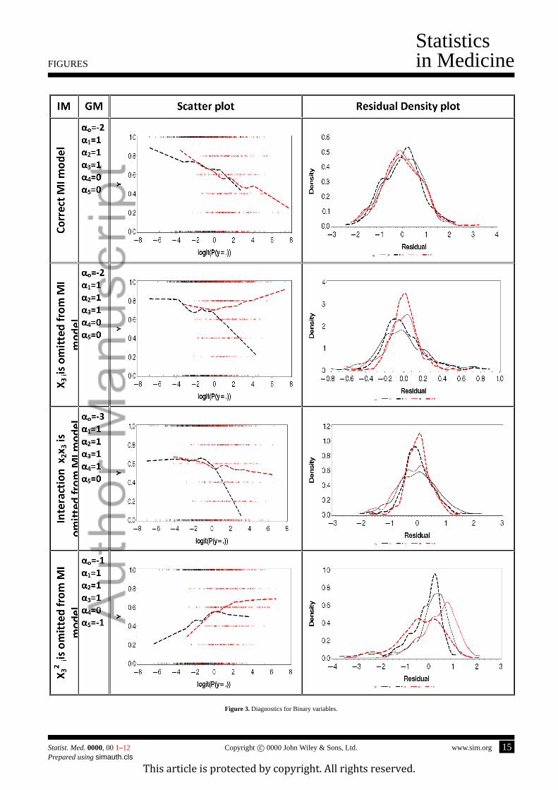
quadratic or interaction terms. The results are illustrated in Figure 3.


The first row corresponds to the correct imputation where the imputation model is consistent with the data generating

model.Scatter Plot Diagnostic, in the first column shows observed (black) and imputed (red) values are very similar.

Residual Density Diagnosticshows a set of four Kernal Density curves. Again the observed values are depicted by the

black lines and the imputed by the red lines. Solid lines of both colors represent observations withy = 0 and dashed lines

representy = 1. The kernel densities in the first row are very similar across all four subgroups. Thus, both diagnostics

confirm the validity of imputations.

The second row of graphs corresponds to the omitted-variable scenario. LOESS curves are clearly different for the

observed and imputed values ofy. For the third row, a case of ignored interaction, theScatter Plot Diagnosticclearly

diagnoses a problem with imputations. On the other hand, theResidual Density Diagnosticare not very informative.

The last row shows a scenario where a square term forx3 is present in the data generation model but is omitted from

the imputation model. Here theScatter Plot Diagnosticis rather ambiguous. LOESS curves for the observed and imputed

values ofy coincide in the area of the most dense overlap of propensities for respondents and nonrespondents, and differ





on the sides. However, residual plot clearly shows the difference in distributions for nonrespondents for whomy was

imputed to be 0 and for those withy imputed as 1. The last two scenarios indicate discrepancy between conclusions from

Scatter Plot DiagnosticandResidual Density Diagnostic. As for the continuous variable, it is important to check both

diagnostic tools to evaluate the imputations.

4.3. Assessment of Uncongeniality

An analyst can detect uncongeniality by constructingScatter Plot Diagnosticand Residual Density Diagnosticusing

the residuals from the analyst model. Suppose that the analyst using a regression model that involvesYv and has some

imputed values. Suppose, that the analyst model was applied to the imputed data setl yielding the residualsr(l). If the

imputations are “agreeable” with the analyst model, then under MAR assumption, in each imputed data setl distribution

of the residualsr(l), conditional on the estimated propensity of response, must be similar forRv = 1 andRv = 0 groups.

To createResidual Density diagnosticfirst regressr(l) on the propensity scoreeobs,−v and construct the residualsu(l)

from this model. Next, or each imputationl generate the Kernel Density Plots foru(l) by Rv. If imputation model is

congenial to the analyst model then the marginal distributions of the residualsu(l) must be similar between the two

groups, respondents and nonrespondents.

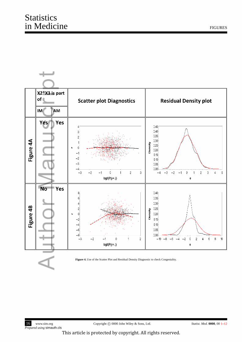
To further elaborate on this approach, we simulated data for the congenial and uncongenial scenarios. Specifically, an

analyst is interested in a regression model fory as a linear function ofx1, x3 and their product. The analyst believes that

interaction betweenx1 andx3 is important. However, the analyst has no knowledge if the interaction was included in the

imputation model and wants to assess if the imputations are valid under the posited model.

We simulated the data under the analyst model, reset some values ofy to missing, and then multiply imputed the two

sets data. One set was imputed incorporating interactionx1 ∙ x3 into the imputation model. The second set was imputed

ignoring the interaction. The Figure 4a shows theScatter PlotandResidual Densitydiagnostics for the congenial models

were imputation model included the interaction. Neither plot shows any differences between distributions for the residuals

based on the observed and imputed values. However, the plots in Figure 4b, corresponding to the imputations omitting

the interaction term, show differences between the observed and imputed values. These differences allow the analyst to

conclude that imputations are not reasonable under the analyst model.


We conducted several other simulation studies varying the missingness rate, alternative models for both regression

model for the outcome as well as missing data mechanism. Across all these simulation studies, the proposed diagnostic

procedure detected modest to severe discrepancies. When the residual variance in the outcome regression model is large

compared to systematic bias due to underfitting, the residual diagnostic plots were better in detecting the problems than

the scatter plot diagnostic. Generally, together they practically identified problems when they exist.

5. Numerical Tests

Though the emphasis of this paper has been on graphical approach, we also propose two test procedures that mirror

the graphical diagnostic tools. These are useful to formally test the validity of imputations using the significance testing

framework.

As indicated earlier, a numeric test analogous to the scatter plot diagnostics can be performed applying the analysis of

variance technique. A similar approach has been used to ensure balance of covariates on the estimated propensity score

[17] . To apply the ANOVA technique to diagnose problems, the estimated probabilities of responseeobs,−v are grouped

intoH strata. The analysis of variance model includes stratum (H − 1 degrees of freedom), indicator for observed/imputed

(1 degree of freedom) and their interactions (H − 1 degrees of freedom) as factors. It has been shown that with five strata




90% of the bias is removed [19, 24] Thus, we useH = 5 as default guidance for this test. The ANOVA test basically

uses a F-statistic that compares the full model with the null model that drops the missing data indicator and stratum by

indicator interaction term.

As a numerical analog of KDE diagnostics, we propose using the Kolmogorov-Smirnov (KS) test for equality of the

distribution of the residuals for the imputed and observed units conditional on the estimated propensity of response. Define

the residualsrsv = ysv − ysv, whereysv is the prediction from the regression ofYv on eobs,−v. Compute the KS statistic

comparing the residuals forRv = 1 with Rv = 0. Thus the ANOVA test would formally test the equality of the location,

and the Kolmogorov-Smirnov (KS) test examines equality of the full residual distribution.

As indicated earlier, due to correlation between the imputed and observed values , the standard sampling distributions for

the ANOVA and KS procedures cannot be applied. It is difficult to analytically derive the actual sampling distributions.

Instead we conducted a simulation study by generating data under both null and non-null scenarios, applied the test

procedures on each multiply imputed data set and determined the cut points under the null scenarios that resulted in the

exact and nominal level to be the same. We then used the same cut points for the non-null scenarios to determine the power

of these tests.

We generated 500 data sets under the simulation scenarios described in Section 4. We also added modest and severe

misspecification. The following table provides the true and imputation models used in the simulation.

[Table 1 about here.]

We calculated the number of rejections of the null hypothesis for each test in every imputed data set. Based on these

empirical distributions, we established a rule based on the number data sets in which the hypothesis should rejected (under

the null model) to ensure that type I error is close to the nominal level (we chose 0.05). For both the tests, the following

two simple rules of rejecting the imputation model worked best:

1. Rule 1: Reject the imputation model if the ANOVA test is rejected in at least two of the five imputed data sets.

2. Rule 2: Reject if at least KS is rejected in at least one of the five imputed data sets or ANOVA test is rejected in at

least two of the five imputed data sets.

Table 2 provides the exact level (under the null) and power (under the alternative) based on the 500 simulated data sets.

[Table 2 about here.]

The results in Table 2 suggest that though using just the ANOVA test may be sufficient to detect large departures from the

true model but using both KS and ANOVA tests add considerable power to detect relatively modest differences between

the true and imputation models.

6. Conclusion

The major emphasis of this paper is to propose a set of graphical diagnostic tools that adopts propensity score methods to

assist in assessing suitability of multiple imputations for an analyst without the full knowledge of the imputation model.

Additionally, the proposed diagnostics can be used by an imputer to check the validity of the imputations from the working

model and refine it, if necessary. The central theme is the comparison of the imputed and observed values conditional on

the estimated propensity of response even with missing values in other variables.

Two proposed diagnostic tools help to evaluate different features of imputed values. The scatter plot diagnostics assist in

comparison of the conditional distributions, whereas the residual density plots are useful in comparison of means as well

as second and third moments of the residual distributions. It is important to address both issues when evaluating multiple

imputations. We also proposed and evaluated some simple rules for rejecting the imputation model using the significance

testing framework.





Although, the focus was on binary and continuous variables, the method could be extended to count or semi-continuous

variables. For example, in the case of semi-continuous variables, the diagnostics can be carried out in two parts. The first

part uses the binary variable diagnostic tools assess the validity of imputations of zero/non-zero status. Next, conditional

on the binary variable being non-zero, one can use the continuous variable approach to assess the validity of imputed

continuous values. The methodology can be easily implemented in standard software packages such as R or Stata and

has already been used in a complex setting [25] where they use limited techniques in the non-peer reviewed technical

report [26]. This report considered mainly continuous variables, did not provide theoretical underpinnings, refinements

for binary variable and the numerical tests. The present article also carries out a more thorough evaluation of the proposed

tools.

The proposed approach can be used by an analyst who was not involved in the imputation process and seeks to assess

congeniality of the imputation and analyst models. If the diagnostic procedures indicate problems with the imputation,

then it may be prudent for the analyst to ignore the imputed values and adopt alternative approaches such as multiple

imputation analysis by re-imputing the missing values in just the variables in the analyst model, the maximum likelihood

or the fully Bayesian analysis. A comparison of the results with original and re-imputed values might be useful to quantify

sensitivity of inferences to model misspecification. Such analysis across the data sets might be useful to assess the impact

of uncongeniality on multiple imputation inferences.

There are number of limitations that can be addressed with further research. First, the approach assumes that the data

set includes all the variables used in the imputation process. In some applications, the imputer may use some internally

available variables and it is possible that our diagnostics may indicate problems where there are none. However, as long as

all variables used in imputations are used in propensity score estimation the inferences should be valid. Second limitation is

the assumption that the data are missing at random. The problems identified by the procedures may be due to nonignorable

missing data mechanism rather than problems with the imputation model. The third limitation is that while focusing on

variableYv, the estimated propensity score is constructed by averaging over imputations of all other variablesY−v. If

the models imputing those variables are severely misspecified, then the estimated propensity score may be affected. One

solution is to apply the diagnostics sequentially and iteratively for all the variables until all the models show reasonable fit

across all variables. Nevertheless, further work is needed to address these limitations.

References

[1] Rubin DB.Multiple Imputation for Nonresponse in Surveys. Wiley, 1987.

[2] Li KH, Raghunathan TE, Rubin D. Large sample significance levels from multiply-imputed data using momentbased

statistics and an f-reference distribution.J. Am. Statist. Assoc.1991;86:1065–1073.

[3] Li KH, Meng X, Raghunathan T, Rubin DB. Significance levels from repeated p-values with multiply imputed data.

Statist. Sinica1991;1:65–92.

[4] Barnard J, Rubin DB. Small-sample degrees of freedom with multiple imputation.Biometrika1999;86(4):948–955.

[5] X L Meng X, Rubin DB. Performing likelihood ratio tests with multiply imputed data sets.Biometrika1995;79:103–

111.

[6] Raghunathan TE, Lepkowski JM, Hoewyk JV, Solenberger P. A multivariate technique for multiply imputing missing

values using a sequence of regression models.Survey methodology2001;27(1):85–95.

[7] Berglund P, Heeringa SH.Multiple Imputation of Missing Data Using SAS. SAS Institute, 2014.

[8] van Buuren S.Flexible Imputation of Missing Data. Chapman and Hall/CRC, 2012.




[9] Stata.Multiple-Imputation Reference Manual. Stata Press, 2015.

[10] Meng XL. Multiple-imputation inferences with uncongenial sources of input.Statistical Science1994;9(4):538–558.

[11] Kim JK, Brick JM, Fuller WA, Kalton G. On the bias of the multiple-imputation variance estimator in survey

sampling.Journal of the Royal Statistical Society: Series B (Statistical Methodology)2006;68(3):509–521.

[12] Robins JM, Wang N. Inference for imputation estimators.Biometrika2000;87(1):113–124.

[13] Aboyomi K, Gelman A, Levy M. Diagnostics for multiple imputations.Applied Statistics2008;57(3):273–291.

[14] He Y, Zaslavsky AM, Harrington DP, Catalano P, Landrum MB. Multiple imputation in a large-scale complex survey:

A practical guide.Stat Methods Med Res.2010;19(6):653670.

[15] Azur MJ, Stuart EA, Frangakis C, Leaf PJ. Multiple imputation by chained equations: What is it and how does it

work?Int J Methods Psychiatr Res.2011;20(1):4049.

[16] Stuart EA, Azur M, Frangakis C, Leaf P. Multiple imputation with large data sets: A case study of the children’s

mental health initiative.Am J Epidemiol2009;169(9):11331139.

[17] Rosenbaum P, Rubin D. The central role of the propensity score in the observational studies for causal effects.

Biometrika1983;70:41–55.

[18] Ralph B D’Agostino J, Rubin DB. Estimating and using propensity scores with partially missing data.JASA2000;

95(451):749–759.

[19] Rosenbaum P, Rubin D. Reducing bias in observational studies using subclassification on the propensity score.

Biometrika1984;79(387):516–524.

[20] Cochran WG, Rubin DB. Controlling bias in observational studies: A review.The Indian Journal of Statistics, Series

A 1973;35(4):417–446.

[21] Hosmer DW, Lemeshow S.Applied logistic regression.Wiley.: New York, 1989.

[22] Rubin DB. Graphical methods for assessing logistic regression models: Comment.Journal of the American

Statistical Association1984;79:7980.

[23] Boonstra P, Bondarenko I, Park S, Voconas P, Mukherjee B. Propensity score-based diagnostics for categorical

response regression models.Statistics in Medecine2014;33(3):455–469.

[24] Cochran W, Rubin DB. Controlling bias in observational studies: a review.Sankhy: The Indian Journal of Statistics,

Series A1973;35:417–446.

[25] Robbins MW, Ghosh SK, Habiger JD. Imputation in high-dimensional economic data as applied to the agricultural

resource management survey.Journal of the American Statistical Association2013;108(501):81–95.

[26] Raghunathan TE, Bondarenko I. Diagnostics for multiple impuation.SSRN Technical Report2007; URLhttp:

//ssrn.com/abstract=1031750 .



http://ssrn.com/abstract=1031750

http://ssrn.com/abstract=1031750

FIGURES


Figure 1. Diagnostics for continuous variables.



Statisticsin Medicine FIGURES

Figure 2. Targets for Scatter Plot and residual Density Diagnostics.

14 www.sim.org Copyrightc© 0000 John Wiley & Sons, Ltd. Statist. Med.0000, 001–12Prepared usingsimauth.cls


FIGURES


Figure 3. Diagnostics for Binary variables.



Statisticsin Medicine FIGURES

Figure 4. Use of the Scatter Plot and Residual Density Diagnostic to check Congeniality.



TABLES


Table 1.True and Imputation models used in determining the exact and power of ANOVA and KS procedures. Residualvariance is 1 for all seven true models

Model Number Type of Model True Model Imputation Model1 Null E(y) = 1 + x1 + x2 + x3 y ∼ N(αo + α1x1 + α2x2 + α3x3, σ

2)2 Omitted E(y) = 1 + x1 + x2 + x3 y ∼ N(αo + α1X1 + α2x2, σ

2)3 variable E(y) = 1 + x1 + x2 + 0.5x3 Same as above4 Interaction E(y) = 1 + x1 + x2 + x3 + x2x3 y ∼ N(αo + α1x1 + α2x2 + α2x3, σ

2)5 omitted E(y) = 1 + x1 + x2 + x3 + 0.5x2x3 same as above6 Square term E(y) = 1 + x1 + x2 + x3 + x2

3 y ∼ N(αo + α1x1 + α2x2 + α3x3, σ2)

7 omitted E(y) = 1 + x1 + x2 + x3 + 0.5x23 Same as above



Statisticsin Medicine TABLES

Table 2.The exact level and power (both in %) based on the two rules for rejecting the imputation model

Model Rule 1 Rule 21 5.2 6.22 98.8 99.43 50.4 64.44 37.8 87.65 36.4 72.86 86.4 1007 13.8 72.2



Graphical and Numerical Diagnostic Tools to Assess ...

Documents

Transcript of Graphical and Numerical Diagnostic Tools to Assess ...