Graph structure learning for network inference:...

Graphstructurelearningfornetworkinference:ModuleNetworks

[email protected]

Computa=onalNetworkBiologyBiosta2s2cs&MedicalInforma2cs826

ComputerSciences838hBps://compnetbiocourse.discovery.wisc.edu

Sep20th2016

SomeofthematerialcoveredinthislectureisadaptedfromBMI576

Goalsforthislecture

•  Per-modulenetworkinferencemethods•  Modulenetworks•  AfewcasestudiesofModulenetworks•  Combiningper-geneandper-modulenetworkinferencemethods(if2mepermits)

Twoclassesofexpression-basednetworkinferencemethods

•  Per-gene/directmethods

•  Modulebasedmethods(Thislecture)

X5X3

X1 X2

Module(Cluster)

X3

X1 X2

X5

X1 X4

Per-modulemethods

•  Findregulatorsforanen2remodule– Assumegenesinthesamemodulehavethesameregulators

•  ModuleNetworks(Segaletal.2005)•  Stochas2cLeMoNe(Joshietal.2008)

Permodule

Y2Y1

X1 X2

Module

ModuleNetworks

•  Mo2va2on:– Mostcomplexsystemshavetoomanyvariables– Notenoughdatatorobustlylearnnetworks–  Largenetworksarehardtointerpret

•  Keyidea:Groupsimilarlybehavingvariablesinto“modules”andlearnthesameparentsandparametersforeachmodule

•  Relevancetogeneregulatorynetworks– Genesthatareco-expressedarelikelyregulatedinsimilarways

Segaletal2005,JMLR

Regulatorygenemodules

Aregulatorymodule:setofgeneswithsimilarregulatorystate

com

men

tre

view

sre

po

rtsd

ep

osite

d re

search

inte

raction

sin

form

ation

refe

reed

rese

arch

http://genomebiology.com/2002/3/11/research/0059.3

Figure 1Many yeast genes are conditionally coregulated. (a) A Venn diagram representing hypothetical genes that are coregulated by transcription factor A (TFA) in response to condition a, transcription factor B (TF B) in response to condition b, or transcription factor C (TF C) in response to condition c. Theregions of overlap in the diagram represent genes that are conditionally coregulated with each respective group of genes (for example, gene 4).(b) Hypothetical gene-expression patterns for four representative genes in groups from (a) show that the expression pattern for gene 4 has similaritiesto the expression patterns of each of the other genes. For this and other diagrams, gene-expression data are represented in a colorized, tabular formatin which each row indicates the relative transcript abundance for a given gene, and each column represents the relative transcript abundance for manygenes as measured in one experiment. A red square indicates that a gene was induced in response to the condition listed, a green square indicates that agene was repressed under those conditions, a black square indicates that there was no detectable change in expression, and a gray square representsmissing data. (c) The gene-expression patterns of around 40 of the 70 known Yap1p targets are shown, as the genes appear in the complete,hierarchically clustered dataset. Because these genes were coordinately induced in response to only subsets of the conditions shown here (labeled inred), the entire set of Yap1p targets was assigned to multiple hierarchical clusters, the largest of which are shown here. The remaining Yap1p targetswere assigned to other hierarchical clusters and are not shown in this display. The colored triangles above the figure represent the microarray timecourses that measured the changes in transcript abundance in response to zinc or phosphate limitation (Zn Pho), treatment with methylmethanesulfonate (MMS), ionizing radiation (IR), heat shock (HS), hydrogen peroxide (H2O2), menadione (MD), dithiothreitol (DTT), diamide (DI), sorbitol(SORB), amino-acid starvation (AA starv), nitrogen starvation (N starv), and progression into stationary phase (STAT). Steady-state gene expression wasalso measured for cells growing on alternative carbon sources (C sources), indicated by the purple rectangle. See text for references.

>4xInduced

>4xRepressed

IRZn P

ho

MM

S

HS

H2O

2

MD

DT

T

DI

SO

RB

AA

sta

rv

N s

tarv

STA

T

C s

ourc

es

Genesregulatedby TF A

Genes regulatedby TF B

Genes regulatedby TF C

Condition a

Condition b

Condition c

Condit

ion a

Condit

ion b

Condit

ion c

Gene 1

Gene 2

Gene 3Gene 4

1

2

3

4

(a)

(c)

(b)

ModulesGenes

Genes

Gasch&Eisen,2002High

expression Low

expression

Experimental conditions

Defini=onofamodule

•  Sta2s2caldefini2on(specifictomodulenetworksbySegal2005)– Asetofrandomvariablesthatshareasta2s2calmodel

•  Biologicaldefini2onofamodule– Setofgenesthatareco-expressedandco-regulated

BayesiannetworkvsModulenetwork

•  Bayesiannetwork– DifferentCPDperrandomvariable– Learningonlyrequirestosearchforparents

•  Modulenetwork– CPDpermodule

•  SameCPDforallrandomvariablesinthesamemodule

– Learningrequiresparentsearchandmodulemembershipassignment

BayesiannetworkvsModulenetworkLEARNING MODULE NETWORKS

INTL

MSFT

MOT

AMAT

DELL HPQ

CPD 4

P(INTL)MSFT

CPD 6CPD 6

CPD 3

CPD 5

CPD 1

CPD 2

INTL

MSFT

MOT

DELL

Module 3

Module 2

Module 1

CPD 3

CPD 2

CPD 1

AMAT

HPQ

(a) Bayesian network (b) Module network

Figure 1: (a) A simple Bayesian network over stock price variables; the stock price of Intel (INTL)is annotated with a visualization of its CPD, described as a different multinomial dis-tribution for each value of its influencing stock price Microsoft (MSFT). (b) A simplemodule network; the boxes illustrate modules, where stock price variables share CPDsand parameters. Note that in a module network, variables in the same module have thesame CPDs but may have different descendants.

to modules and the probabilistic model for each module. We evaluate the performance of our al-gorithm on two real data sets, in the domains of gene expression and the stock market. Our resultsshow that our learned module network generalizes to unseen test data much better than a Bayesiannetwork. They also illustrate the ability of the learned module network to reveal high-level structurethat provides important insights.

2. The Module Network Framework

We start with an example that introduces the main idea of module networks and then provide aformal definition. For concreteness, consider a simple toy example of modeling changes in stockprices. The Bayesian network of Figure 1(a) describes dependencies between different stocks. Inthis network, each random variable corresponds to the change in price of a single stock. For illus-tration purposes, we assume that these random variables take one of three values: ‘down’, ‘same’or ‘up’, denoting the change during a particular trading day. In our example, the stock price ofIntel (INTL) depends on that of Microsoft (MSFT). The conditional probability distribution (CPD)shown in the figure indicates that the behavior of Intel’s stock is similar to that of Microsoft. Thatis, if Microsoft’s stock goes up, there is a high probability that Intel’s stock will also go up and viceversa. Overall, the Bayesian network specifies a CPD for each stock price as a stochastic functionof its parents. Thus, in our example, the network specifies a separate behavior for each stock.

The stock domain, however, has higher order structural features that are not explicitly modeledby the Bayesian network. For instance, we can see that the stock price of Microsoft (MSFT) in-

559

Eachvariabletakesthreevalues:UP,DOWN,SAME

Modelingques=onsinModuleNetworks

•  Howtoscoreandlearnmodulenetworks?•  HowtomodeltheCPDbetweenparentandchildren?– RegressionTree

DefiningaModuleNetwork

•  Aprobabilis2cgraphicalmodeloverNrandomvariables

•  SetofmodulevariablesM1.. MK•  ModuleassignmentsA thatspecifiesthemodule(1-to-K) foreachXi

•  CPDpermoduleP(Mj|PaMj), PaMjareparentsofmodule Mj– EachvariableXiinMjhasthesamecondi2onaldistribu2on

X = {X1, · · · , XN}

LearningaModuleNetwork

•  Giventrainingdataset ,fixednumberofmodules(K)

•  Learn– ModuleassignmentsAofeachvariabletoamodule

– TheparentsofeachmodulegivenbystructureS

D = {x1, · · · ,xm}

Scoreofamodulenetwork

•  ModulenetworkmakesuseofaBayesianscore

SEGAL, PE’ER, REGEV, KOLLER AND FRIEDMAN

For example, in the case of networks that use only multinomial table CPDs, we have one suffi-cient statistic function for each joint assignment x ∈ Val(M j),u ∈ Val(PaM j), which is

${Xi[m] = x,paM j [m] = u},

the indicator function that takes the value 1 if the event (Xi[m] = x,PaM j [m] = u) holds, and 0otherwise. The statistic on the data is

S j[x,u] =M

#m=1

#Xi∈X j

${Xi[m] = x,PaM j [m] = u}.

Given these sufficient statistics, the formula for the module likelihood function is:

Lj(PaM j ,X j,!M j|PaM j:D) = "

x,u∈Val(M j,PaM j )

!S j[x,u]x|u .

This term is precisely the one we would use in the likelihood of Bayesian networks with multinomialtable CPDs. The only difference is that the vector of sufficient statistics for a local likelihood termis pooled over all the variables in the corresponding module.

For example, consider the likelihood function for the module network of Figure 1(b). In thisnetwork we have three modules. The first consists of a single variable and has no parents, and sothe vector of statistics S[M1] is the same as the statistics of the single variable S[MSFT]. The secondmodule contains three variables; thus, the sufficient statistics for the module CPD is the sum of thestatistics we would collect in the ground Bayesian network of Figure 1(a):

S[M2,MSFT] = S[AMAT,MSFT]+ S[MOT,MSFT]+ S[INTL,MSFT].

Finally,S[M3,AMAT, INTL] = S[DELL,AMAT, INTL]+ S[HPQ,AMAT, INTL].

An illustration of the decomposition of the likelihood and the associated sufficient statistics usingthe plate model is shown in Figure 2.

As usual, the decomposition of the likelihood function allows us to perform maximum likeli-hood or MAP parameter estimation efficiently, optimizing the parameters for each module sepa-rately. The details are standard (Heckerman, 1998), and are thus omitted.

3.2 Priors and the Bayesian Score

As we discussed, our approach for learning module networks is based on the use of a Bayesianscore. Specifically, we define a model score for a pair (S ,A) as the posterior probability of thepair, integrating out the possible choices for the parameters !. We define an assignment prior P(A),a structure prior P(S | A) and a parameter prior P(! | S ,A). These describe our preferences overdifferent networks before seeing the data. By Bayes’ rule, we then have

P(S ,A | D) % P(A)P(S | A)P(D | S ,A),

where the last term is the marginal likelihood

P(D | S ,A) =Z

P(D | S ,A ,!)P(! | S)d!.

564

LEARNING MODULE NETWORKS

We define the Bayesian score as the log of P(S ,A | D), ignoring the normalization constant

score(S ,A : D) = logP(A)+ logP(S | A)+ logP(D | S ,A). (3)

As with Bayesian networks, when the priors satisfy certain conditions, the Bayesian score de-composes. This decomposition allows to efficiently evaluate a large number of alternatives. Thesame general ideas carry over to module networks, but we also have to include assumptions thattake the assignment function into account. Following is a list of conditions on the prior required forthe decomposability of the Bayesian score in the case of module networks:

Definition 7 Let P(!,S ,A) be a prior over assignments, structures, and parameters.

• P(!,S ,A) is globally modular if

P(! | S ,A) = P(! | S),

and

P(S ,A) % &(S)'(A)C(A ,S),

where &(S) and '(A) are non-negative measures over structures and assignments, andC(A ,S)is a constraint indicator function that is equal to 1 if the combination of structure and assign-ment is a legal one (i.e., the module graph induced by the assignment A and structure S isacyclic), and 0 otherwise.

• P(! | S) satisfies parameter independence if

P(! | S) =K

"j=1

P(!M j|PaM j| S).

• P(! | S) satisfies parameter modularity if

P(!M j|PaM j| S1) = P(!M j|PaM j

| S2).

for all structures S1 and S2 such that PaS1M j

= PaS2M j.

• &(S) satisfies structure modularity if

&(S) ="j& j(S j),

where S j denotes the choice of parents for moduleM j and & j is a non-negative measure overthese choices.

• '(A) satisfies assignment modularity if

'(A) ="j' j(A j),

where A j denote is the choice of variables assigned to module M j and ' j is a non-negativemeasure over these choices.

565


We define the Bayesian score as the log of P(S ,A | D), ignoring the normalization constant

score(S ,A : D) = logP(A)+ logP(S | A)+ logP(D | S ,A). (3)

As with Bayesian networks, when the priors satisfy certain conditions, the Bayesian score de-composes. This decomposition allows to efficiently evaluate a large number of alternatives. Thesame general ideas carry over to module networks, but we also have to include assumptions thattake the assignment function into account. Following is a list of conditions on the prior required forthe decomposability of the Bayesian score in the case of module networks:

Definition 7 Let P(!,S ,A) be a prior over assignments, structures, and parameters.

• P(!,S ,A) is globally modular if

P(! | S ,A) = P(! | S),

and

P(S ,A) % &(S)'(A)C(A ,S),

where &(S) and '(A) are non-negative measures over structures and assignments, andC(A ,S)is a constraint indicator function that is equal to 1 if the combination of structure and assign-ment is a legal one (i.e., the module graph induced by the assignment A and structure S isacyclic), and 0 otherwise.

• P(! | S) satisfies parameter independence if

P(! | S) =K

"j=1

P(!M j|PaM j| S).

• P(! | S) satisfies parameter modularity if

P(!M j|PaM j| S1) = P(!M j|PaM j

| S2).

for all structures S1 and S2 such that PaS1M j

= PaS2M j.

• &(S) satisfies structure modularity if

&(S) ="j& j(S j),

where S j denotes the choice of parents for moduleM j and & j is a non-negative measure overthese choices.

• '(A) satisfies assignment modularity if

'(A) ="j' j(A j),

where A j denote is the choice of variables assigned to module M j and ' j is a non-negativemeasure over these choices.

565

Priors Datalikelihood

PriorsDatalikelihood

Definingthedatalikelihood

Lj =|D|Y

m=1

Y

Xi�Xj

P (xi[m]|paMj[m], �j)

K:numberofmodules,Xj:jthmodule PaMj ParentsofmoduleMj

Likelihoodofmodulej =KY

j=1

Lj(PaMj ,Xj , �j : D)

Xj = {Xi 2 X|A(Xi) = j}

DatalikelihoodexampleLEARNING MODULE NETWORKS

Instance 3

Module 3

Module 2

Module 1

AMAT

θθθθ

θθθθ

θθθθ

DELL HPQ

INTL

MOT

MSFT

Instance 1

Instance 2

+MSFT)(AMAT,S

+MSFT)(MOT,S

MSFT)(INTL,S

=MSFT),(MS (MSFT)S)(MS =

+INTL)AMAT,(DELL,S

+INTL)AMAT,(HPQ,S

=INTL)AMAT,,(MS

Figure 2: Shown is a plate model for three instances of the module network example of Figure 1(b).The CPD template of each module is connected to all variables assigned to that module(e.g. θM2|MSFT is connected to AMAT, MOT, and INTL). The sufficient statistics ofeach CPD template are the sum of the sufficient statistics of each variable assigned to themodule and the module parents.

module likelihoods, each of which can be calculated independently and depends only on the valuesof X j and PaM j , and on the parameters θM j|PaM j

:

L(M :D)

=K

∏j=1

!

M

∏m=1

∏Xi∈X j

P(xi[m] | paM j [m],θM j|PaM j)

"

=K

∏j=1

Lj(PaM j ,Xj,θM j|PaM j

:D). (1)

If we are learning conditional probability distributions from the exponential family (e.g., discretedistribution, Gaussian distributions, and many others), then the local likelihood functions can bereformulated in terms of sufficient statistics of the data. The sufficient statistics summarize therelevant aspects of the data. Their use here is similar to that in Bayesian networks (Heckerman,1998), with one key difference. In a module network, all of the variables in the same moduleshare the same parameters. Thus, we pool all of the data from the variables in X j, and calculateour statistics based on this pooled data. More precisely, let S j(Mj,PaM j) be a sufficient statisticfunction for the CPD P(Mj | PaM j). Then the value of the statistic on the data set D is

S j =M

∑m=1

∑Xi∈X j

S j(xi[m],paM j [m]). (2)

563

ModulenetworklearningalgorithmLEARNING MODULE NETWORKS

Input:D // Data setK // Number of modules

Output:M // A module network

Learn-Module-NetworkA0 = cluster X into K modulesS0 = empty structureLoop t = 1,2, . . . until convergence

St = Greedy-Structure-Search(At−1,St−1)At = Sequential-Update(At−1,St );

Return M= (At ,St)

Figure 4: Outline of the module network learning algorithm. Greedy-Structure-Search successivelyapplies operators that change the structure as long as each such operator results in a legalstructure and improves the module network score

prove the score. Hence, it converges to a local maximum, in the sense that no single assignmentchange can improve the score.

The computation of the score is the most expensive step in the sequential algorithm. Once again,the decomposition of the score plays a key role in reducing the complexity of this computation:When reassigning a variable Xi from one module Mold to another Mnew, only the local scores ofthese modules change. The module score of all other modules remains unchanged. The rescoring ofthese two modules can be accomplished efficiently by subtracting Xi’s statistics from the sufficientstatistics of Mold and adding them to those of Mnew. Thus, assuming that we have precomputedthe sufficient statistics associated with every pair of variable Xi and moduleM j, the cost of recom-puting the delta-score for an operator is O(s), where s is the size of the table of sufficient statisticsfor a module. The only operators whose delta-scores change are those involving reassignment ofvariables to/from these two modules. Assuming that each module has approximately O(n/K) vari-ables, and we have at most K possible destinations for reassigning each variable, the total numberof such operators is generally linear in n. Thus, the cost of each reassignment step is approximatelyO(ns). In addition, at the beginning of the module reassignment step, we must initialize all of thesufficient statistics at a cost of O(Mnd), and compute all of the delta-scores at a cost of O(nK).

4.3 Algorithm Summary

To summarize, our algorithm starts with an initial assignment of variables to modules. In general,this initial assignment can come from anywhere, and may even be a random guess. We choose toconstruct it using the clustering-based idea described in the previous section. The algorithm theniteratively applies the two steps described above: learning the module dependency structures, and re-assigning variables to modules. These two steps are repeated until convergence, where convergenceis defined by a score improvement of less than some fixed threshold ! between two consecutivelearned models. An outline of the module network learning algorithm is shown in Figure 4.

Each of these two steps — structure update and assignment update — is guaranteed to eitherimprove the score or leave it unchanged. The following result therefore follows immediately:

571

Ini=almodulesiden=fiedbyexpressionclustering

M1

M2

M3

Cluster

Gene

s

Experiments

Itera=onsinlearningModuleNetworksLearnregulators/CPDpermodule

X1

X3X4

X5 X6

X2M1

M2

M3

X1X2

X3X4

X5X6X7X8 X7 X8

X5 X6

X4 X1

X1

X3X4

X5 X6

X2

X7

X8

X5 X6

X4 X1

Revisitthemodules

M1

M2

M3X8

ModuleM1andM3getupdated

Moduleassignmentsearch

•  Happensintwoplaces•  Moduleini2aliza2on–  Interpretasclusteringoftherandomvariables

•  Modulere-assignment

X = {X1, · · · , XN}

Moduleini=aliza=onasclusteringofvariables


1.61.3-10.21.5-1.4

-3.5-2.94-0.2-3.24.1

1.21.3-0.80.11.1-1.1

-4-3.13.9-0.2-2.93.2

1.61.3-10.21.5-1.4

-3.5-2.94-0.2-3.24.1

1.21.3-0.80.11.1-1.1

-4-3.13.9-0.2-2.93.2x[1]

DELL

MSFT

AMAT

MOT

HPQ

INTL

x[2]

x[3]

x[4] 1.61.3-10.21.5-1.4

1.21.3-0.80.11.1-1.1

-3.5-2.94-0.2-3.24.1

-4-3.13.9-0.2-2.93.2

1.61.3-10.21.5-1.4

1.21.3-0.80.11.1-1.1

-3.5-2.94-0.2-3.24.1

-4-3.13.9-0.2-2.93.2x[1]

DELL

MSFT

AMAT

MOT

HPQ

INTL

x[3]

x[2]

x[4]

1

2-1-1.41.61.31.50.2

44.1-3.5-2.9-3.2-0.2

-0.8-1.11.21.31.10.1

3.93.2-4-3.1-2.9-0.2

-1-1.41.61.31.50.2

44.1-3.5-2.9-3.2-0.2

-0.8-1.11.21.31.10.1

3.93.2-4-3.1-2.9-0.2x[1]

MSFT

MOT

HPQ

DELL

AMAT

INTL

x[2]

x[3]

x[4]

1 2 3

(a) Data (b) Standard clustering (c) Initialization

Figure 5: Relationship between the module network procedure and clustering. Finding an assign-ment function can be viewed as a clustering of the variables whereas clustering typicallyclusters instances. Shown is sample data for the example domain of Figure 1, wherethe rows correspond to instances and the columns correspond to variables. (a) Data. (b)Standard clustering of the data in (a). Note that x[2] and x[3] were swapped to form theclusters. (c) Initialization of the assignment function for the module network procedurefor the data in (a). Note that variables were swapped in their location to reflect the initialassignment into three modules.

Theorem 4.1: The iterative module network learning algorithm converges to a local maximum ofscore(S ,A : D).

We note that both the structure search step and the module reassignment step are done usingsimple greedy hill-climbing operations. As in other settings, this approach is liable to get stuck inlocal maxima. We attempt to somewhat compensate for this limitation by initializing the search ata reasonable starting point, but local maxima are clearly still an issue. An additional strategy thatwould help circumvent some maxima is the introduction of some randomness into the search (e.g.,by random restarts or simulated annealing), as is often done when searching complex spaces withmulti-modal target functions.

5. Learning with Regression Trees

We now briefly review the family of conditional distributions we use in the experiments below.Many of the domains suited for module network models contain continuous valued variables, suchas gene expression or price changes in the stock market. For these domains, we often use a condi-tional probability model represented as a regression tree (Breiman et al., 1984). For our purposes,a regression tree T for P(X | U) is defined via a rooted binary tree, where each node in the tree iseither a leaf or an interior node. Each interior node is labeled with a test U < u on some variableU ∈ U and u ∈ IR. Such an interior node has two outgoing arcs to its children, corresponding to theoutcomes of the test (true or false). The tree structure T captures the local dependency structure ofthe conditional distribution. The parameters of T are the distributions associated with each leaf. Inour implementation, each leaf ℓ is associated with a univariate Gaussian distribution over values ofX , parameterized by a mean µℓ and variance !2ℓ . An example of a regression tree CPD is shown in

572

formodulenetwork

Modulere-assignment

•  Mustpreservetheacyclicgraphstructure•  Mustimprovescore•  Modulere-assignmenthappensusingasequen&alupdateprocedure:– Updateonlyonevariableata2me– Thechangeinscoreofmovingavariablefromonemoduletoanotherwhilekeepingtheothervariablesfixed

Modulere-assignmentviasequen=alupdate


Input:D // Data setA0 // Initial assignment functionS // Given dependency structure

Output:A // improved assignment function

Sequential-UpdateA = A0LoopFor i= 1 to nFor j = 1 to K

A ′ = A except that A ′(Xi) = jIf ⟨GM ,A ′⟩ is cyclic, continueIf score(S ,A ′ : D) > score(S ,A : D)

A = A ′

Until no reassignments to any of X1, . . .XnReturn A

Figure 3: Outline of sequential algorithm for finding the module assignment function

4.2.3 MODULE REASSIGNMENT

In the module reassignment step, the task is more complex. We now have a given structure S , andwish to find A = argmaxA ′scoreM(S ,A ′ : D). We thus wish to take each variable Xi, and select theassignment A(Xi) that provides the highest score.

At first glance, we might think that we can decompose the score across variables, allowingus to determine independently the optimal assignment A(Xi) for each variable Xi. Unfortunately,this is not the case. Most obviously, the assignments to different variables must be constrainedso that the module graph remains acyclic. For example, if X1 ∈ PaMi and X2 ∈ PaM j , we cannotsimultaneously assign A(X1) = j and A(X2) = i. More subtly, the Bayesian score for each moduledepends non-additively on the sufficient statistics of all the variables assigned to the module. (Thelog-likelihood function is additive in the sufficient statistics of the different variables, but the logmarginal likelihood is not.) Thus, we can only compute the delta score for moving a variable fromone module to another given a fixed assignment of the other variables to these two modules.

We therefore use a sequential update algorithm that reassigns the variables to modules one byone. The idea is simple. We start with an initial assignment function A0, and in a “round-robin”fashion iterate over all of the variables one at a time, and consider changing their module assignment.When considering a reassignment for a variable Xi, we keep the assignments of all other variablesfixed and find the optimal legal (acyclic) assignment for Xi relative to the fixed assignment. Wecontinue reassigning variables until no single reassignment can improve the score. An outline ofthis algorithm appears in Figure 3

The key to the correctness of this algorithm is its sequential nature: Each time a variable as-signment changes, the assignment function as well as the associated sufficient statistics are updatedbefore evaluating another variable. Thus, each change made to the assignment function leads to alegal assignment which improves the score. Our algorithm terminates when it can no longer im-

570

Modelingques=onsinModuleNetworks

•  Howtoscoreandlearnmodulenetworks?•  HowtomodeltheCPDbetweenparentandchildren?– RegressionTree

Represen=ngtheCondi=onalprobabilitydistribu=on

•  Xiarecon2nuousvariables•  Howtorepresentthedistribu2onofXi giventhestateofitsparents?

•  Howtocapturecontext-specificdependencies?

•  Modulenetworksusearegressiontree

Modelingtherela=onshipbetweenregulatorsandtargets

•  supposewehaveasetof(8)genesthatallhaveintheirupstreamregionsthesameac2vator/repressorbindingsites

Aregressiontree

•  ArootedbinarytreeT•  Eachnodeinthetreeiseitheraninteriornodeoraleafnode

•  InteriornodesarelabeledwithabinarytestXi<u, u isarealnumberobservedinthedata

•  Leafnodesareassociatedwithunivariatedistribu2onsofthechild

AnexampleregressiontreeforaModulenetwork


AMAT<5%

INTL<4%

00000

false

truefalse

true

INTL

MSFT

MOT

DELL

Module 3

Module 2

Module 1

AMAT

HPQ

P(M3 | AMAT, INTL)

N(1.4,0.8) N(0.1,1.6) N(-2,0.7)

Figure 6: Example of a regression tree with univariate Gaussian distributions at the leaves for rep-resenting the CPD P(M3 | AMAT, INTL), associated withM3. The tree has internal nodeslabeled with a test on the variable (e.g. AMAT < 5%). Each univariate Gaussian distri-bution at a leaf is parameterized by a mean and a variance. The tree structure capturesthe local dependency structure of the conditional distributions. In the example shown,when AMAT ≥ 5%, then the distribution over values of variables assigned toM3 will beGaussian with mean 1.4 and standard deviation 0.8 regardless of the value of INTL.

Figure 6. We note that, in some domains, Gaussian distributions may not be the appropriate choiceof models to assign at the leaves of the regression tree. In such cases, we can apply transforma-tions to the data to make it more appropriate for modeling by Gaussian distributions, or use othercontinuous or discrete distributions at the leaves.

To learn module networks with regression-tree CPDs, we must extend our previous discus-sion by adding another component to S that represents the trees T1, . . . ,TK associated with the dif-ferent modules. Once we specify these components, the above discussion applies with severalsmall differences. These issues are similar to those encountered when introducing decision trees toBayesian networks (Chickering et al., 1997; Friedman and Goldszmidt, 1998), so we discuss themonly briefly.

Given a regression tree Tj for P(M j | PaM j), the corresponding sufficient statistics are the statis-tics of the distributions at the leaves of the tree. For each leaf ℓ in the tree, and for each data instancex[m], we let ℓ j[m] denote the leaf reached in the tree given the assignment to PaM j in x[m]. The mod-ule likelihood decomposes as a product of terms, one for each leaf ℓ. Each term is the likelihood forthe Gaussian distribution N

!

µℓ;+2ℓ"

, with the usual sufficient statistics for a Gaussian distribution.Given a regression tree Tj for P(M j | PaM j), the corresponding sufficient statistics are the statis-

tics of the distributions at the leaves of the tree. For each leaf ℓ in the tree, and for each data instancex[m], we let ℓ j[m] denote the leaf reached in the tree given the assignment to PaM j in x[m]. The mod-ule likelihood decomposes as a product of terms, one for each leaf ℓ. Each term is the likelihood for

573

Module3valuesaremodeledusingGaussiansateachleafnode

Averysimpleregressiontree

X2

X3

e1 e2

µ1,�1

µ2,�2

µ3,�3

X2 > e1

X2 > e2

YESNO

NO YES

µ3,�3µ2,�2µ1,�1

X3

AregressiontreetocaptureaCPD

X1 > e1

X2 > e2

YES

NO

NO YESLeaf

Interiornode

P (X3|X1, X2)

X3 ⇠ N (µ31,�31) X3 ⇠ N (µ32,�32) X3 ⇠ N (µ33,�33)

X3

X1 X2

ExpressionofgenerepresentedbyX3modeledusingGaussiansateachleafnode

e1,e2arevaluesseeninthedata

Algorithmforgrowingaregressiontree

•  Input:datasetD,childvariableXi,candidateparentsCi of Xi

•  Output:TreeT•  Ini2alizeTtoaleafnode,es2matedfromallsamplesofXi

•  Whilenotconverged–  ForeveryleafnodelinT

•  Findwiththebestsplitatl•  Ifsplitimprovesscore

–  addtwoleafnodes,iandjbelowl–  Updatesamplesandparametersassociatedwith,iandj

µ,�

Xj 2 Ci

Learningaregressiontree•  AssumewearesearchingfortheparentsofavariableX3 anditalreadyhastwoparentsX1and X2

•  X4 willbeconsideredusing“split”opera2onsofexis2ngleafnodes

X1 > e1

X2 > e2

YES

NO

NO YES

X4 > e3

NO YES

X1 > e1

X2 > e2

YES

NO

NO YES

N1 N2N3

Nl: Gaussianassociatedwithleafl

N2N3

N4 N5

Convergenceinregressiontreedependson

•  Depthoftree•  Improvementinscore•  Maximumnumberofparents•  Minimumnumberofsamplesperleafnode

AssessingthevalueofusingModuleNetworks

•  Usingsimulateddata–  Generatedatafromaknownmodulenetwork–  Knownmodulenetworkwasinturnlearnedfromrealdata

•  10modules,500variables–  Evaluateusing

•  Testdatalikelihood•  Recoveryoftrueparent-childrela2onshipsarerecoveredinlearnedmodulenetwork

•  Usinggeneexpressiondata–  Externalvalida2onofmodules(Geneontology,mo2fenrichment)

–  Cross-checkwithliterature

TestdatalikelihoodLEARNING MODULE NETWORKS

-800

-750

-700

-650

-600

-550

-500

-450

0 20 40 60 80 100 120 140 160 180 200

Number of Modules

Test

Dat

a Lo

g Li

kelih

ood

(per

inst

ance

)

25 50100 200500

-600

-575

-550

-525

-500

-475

-450

0 20 40 60 80 100

Number of modules

Trai

nnin

g D

ata

Scor

e (p

er in

stan

ce)

25 50100 200500

(a) (b)

Figure 7: Performance of learning from synthetic data as a function of the number of modules andtraining set size. The x-axis corresponds to the number of modules, each curve corre-sponds to a different number of training instances, and each point shows the mean andstandard deviations from the 10 sampled data sets. (a) Log-likelihood per instance as-signed to held-out data. (b) Average score per instance on the training data.

to a specification of the total number of modules. We used regression trees as the local probabilitymodel for all modules, and uniform priors for !(S) and "(A). For structure search, we used beamsearch, using a lookahead of three splits to evaluate each operator. When learning Bayesian net-works, as a comparison, we used precisely the same structure learning algorithm, simply treatingeach variable as its own module.

6.1 Synthetic Data

As a basic test of our procedure in a controlled setting, we used synthetic data generated by a knownmodule network. This gives a known ground truth to which we can compare the learned models.To make the data realistic, we generated synthetic data from a model that was learned from thegene expression data set described below. The generating model had 10 modules and a total of35 variables that were a parent of some module. From the learned module network, we selected500 variables, including the 35 parents. We tested our algorithm’s ability to reconstruct the networkusing different numbers of modules; this procedure was run for training sets of various sizes rangingfrom 25 instances to 500 instances, each repeated 10 times for different training sets.

We first evaluated the generalization to unseen test data, measuring the likelihood ascribed bythe learned model to 4500 unseen instances. The results, summarized in Figure 7(a), show that, forall training set sizes, except the smallest one with 25 instances, the model with 10 modules performsthe best. As expected, models learned with larger training sets do better; but, when run using thecorrect number of 10 modules, the gain of increasing the number of data instances beyond 100samples is small and beyond 200 samples is negligible.

575

Eachlinetyperepresentssizeoftrainingdata

10Modulesisthebestforalmostalltrainingdatasetsizes

Recoveryofgraphstructure


10

20

30

40

50

60

70

80

90

100

0 20 40 60 80 100 120 140 160 180 200

Number of Modules

Frac

tion

of V

aria

bles

in 1

0 La

rges

t Mod

ules

2550100200500

0

10

20

30

40

50

60

70

80

90

0 20 40 60 80 100 120 140 160 180 200

Number of Modules

Rec

over

ed S

truct

ure

(% C

orre

ct)

25 50100 200500

(a) (b)

Figure 8: (a) Fraction of variables assigned to the 10 largest modules. (b) Average percentage ofcorrect parent-child relationships recovered (fraction of parent-child relationships in thetrue model recovered in the learned model) when learning from synthetic data for modelswith various number of modules and different training set sizes. The x-axis correspondsto the number of modules, each curve corresponds to a different number of training in-stances, and each point shows the mean and standard deviations from the 10 sampled datasets.

To test whether we can use the score of the model to select the number of modules, we alsoplotted the score of the learned model on the training data (Figure 7(b)). As can be seen, when thenumber of instances is small (25 or 50), the model with 10 modules achieves the highest score andfor a larger number of instances, the score does not improve when increasing the number of modulesbeyond 10. Thus, these results suggest that we can select the number of modules by choosing themodel with the smallest number of modules from among the highest scoring models.

A closer examination of the learned models reveals that, in many cases, they are almost a 10-module network. As shown in Figure 8(a), models learned using 100, 200, or 500 instances and upto 50 modules assigned ≥ 80% of the variables to 10 modules. Indeed, these models achieved highperformance in Figure 7(a). However, models learned with a larger number of modules had a widerspread for the assignments of variables to modules and consequently achieved poor performance.

Finally, we evaluated the model’s ability to recover the correct dependencies. The total num-ber of parent-child relationships in the generating model was 2250. For each model learned, wereport the fraction of correct parent-child relationships it contains. As shown in Figure 8(b), ourprocedure recovers 74% of the true relationships when learning from a data set with 500 instances.Once again, we see that, as the variables begin fragmenting over a large number of modules, thelearned structure contains many spurious relationships. Thus, our results suggest that, in domainswith a modular structure, statistical noise is likely to prevent overly detailed learned models suchas Bayesian networks from extracting the commonality between different variables with a sharedbehavior.

576

Goalsforthislecture

•  Per-modulenetworkinferencemethods•  Modulenetworks•  AfewcasestudiesofModulenetworks•  Combiningper-geneandper-modulenetworkinferencemethods

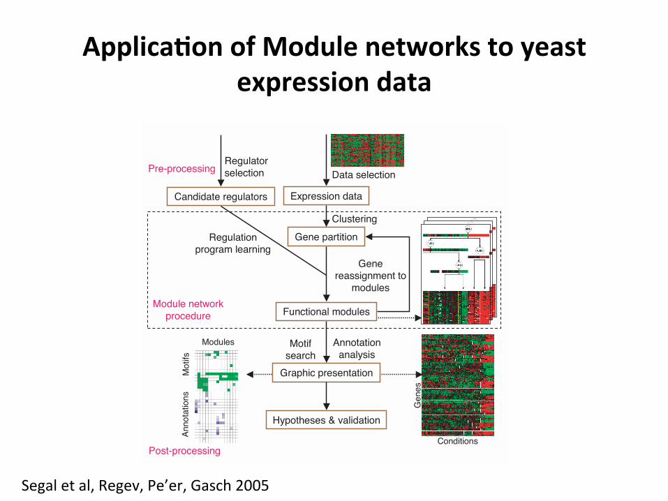
Applica=onofModulenetworkstoyeastexpressiondata A R T I C L E S

NATURE GENETICS VOLUME 34 | NUMBER 2 | JUNE 2003 167

Figure 2 Regulation programs represent context-specific and combinatorialregulation. Shown is a scheme depicting three distinct modes of regulationfor a group of genes. (a) Context A. Genes in the module are not undertranscriptional regulation and are in their basal expression level. (b) ContextB. An activator gene is upregulated and, as a result, binds the upstreamregions of the module genes, thereby inducing their transcription. (c) ContextC. A repressor gene is upregulated and, as a result, blocks transcription of thegenes in the module, thereby reducing their expression levels. (d) A regulationtree or program can represent the different modes of regulation describedabove. Each node in the tree consists of a regulatory gene (for example,‘Activator’) and a query on its qualitative value, in which an upward arrow(red) denotes the query “is gene upregulated?” and a downward arrow (green)denotes the query “is gene downregulated?”. Right branches representinstances for which the answer to the query in the node is ‘true’; left branchesrepresent instances for which the answer is ‘false’. The expression of theregulatory genes themselves is shown below their respective node. Each leafof the regulation tree is a regulation context (bordered by black dotted lines)as defined by the queries leading to the leaf. The contexts partition the arraysinto disjoint sets, where each context includes the arrays defined by thequeries of the inputs that define the context. In context A, the activator is notupregulated and the genes in the module are in their basal expression level(left leaf). In contexts B and C, the activator is upregulated. In context C, the repressor is also upregulated and the module genes are repressed (right leaf).In context B, the repressor is not upregulated and the activator induces expression of the module genes (center leaf). This regulation program specifiescombinatorial interaction; for example, in context B, the module genes are upregulated only when the activator is upregulated but the repressor is not.

of the module’s genes contained the known motif in their upstreamregions). Overall, our results provide a global view of the yeasttranscriptional network, including many instances in which ourmethod identifies known functional modules and their correct reg-ulators, showing its ability to derive regulation from expression.

A regulation program specifies that certain genes regulate certainprocesses under certain conditions. Our method thus generatesdetailed, testable hypotheses, suggesting specific roles for a regulatorand the conditions under which it acts. We tested experimentally the

computational predictions for three putative regulators withunknown functions (a transcription factor and two signaling mole-cules). Our method’s results make specific predictions regarding theconditions under which these regulators operate. Using microarrayanalysis, we compared the transcriptional responses of the respectivegenetically disrupted strains with their congenic wild-types underthese conditions. Deletion of each of the three regulators caused amarked impairment in the expression of a substantial fraction of theircomputationally predicted targets, supporting the method’s predic-tions and giving important insight regarding the function of theseuncharacterized regulators.

RESULTSWe compiled a list of 466 candidate regulators and applied our proce-dure to 2,355 genes in the 173 arrays of the yeast stress data set3,resulting in automatic inference of 50 modules. We analyzed each ofthe resultant modules (Fig. 1) using a variety of external data sources,evaluating the functional coherence of its gene products and thevalidity of its regulatory program.

Sample modulesWe first present in detail several of the inferred modules, selected toshow the method’s ability to reproduce diverse features of regulatoryprograms.

The respiration module (Fig. 3) is a clear example of a predictedmodule and of the validation process. It consists primarily of genesencoding respiration proteins (39 of 55) and glucose-metabolism reg-ulators (6 of 55). The inferred regulatory program specifies the Hap4transcription factor as the module’s top (activating) regulator, pri-marily under stationary phase (a growth phase in which nutrients,primarily glucose, are depleted). This prediction is consistent with theknown role of Hap4 in activation of respiration1,19. Indeed, our post-analysis detected a Hap4-binding DNA sequence motif (bound by theHap2/3/4/5 complex) in the upstream region of 29 of 55 genes in themodule (P < 2 ! 10–13). This motif also appears in non-respirationgenes (mitochondrial genes and glucose-metabolism regulators),which, together with their matching expression profiles, supportstheir inclusion as part of the module. When Hap4 is not induced, the

Data selection

Expression dataCandidate regulators

Regulatorselection

Gene partitionClustering

Functional modules

Graphic presentation

Hypotheses & validation

Gene reassignment to

modules

Annotation analysis

Motifsearch

Regulation program learning

Pre-processing

Module networkprocedure

Post-processing

Modules

Mot

ifsAn

nota

tions

Conditions

Gen

es

Figure 1 Overview of the module networks algorithm and evaluationprocedure. The procedure takes as input a data set of gene expressionprofiles and a large precompiled set of candidate control genes. The methoditself (dotted box) is an iterative procedure that determines both the partitionof genes to modules and the regulation program (right icon in dotted box) foreach module. In a post-processing phase, modules are tested for enrichmentof gene annotations and cis-regulatory binding site motifs.

dActivator

TrueFalse

TrueFalse

Contex

t A

Contex

t B

Contex

t C

Target gene expression

Repressor expression

Mod

ule

gene

sR

egul

atio

n pr

ogra

m

Activator expression

Induced

Repressed

Repressorbinding site

Upstream regionof target gene

a

b

cRepressor

Activator

Activatorbinding site

Activatorbinding site

Activator

Context A

Context B

Transcriptlevel

Context C

Repressor

©20

03 N

atur

e Pu

blis

hing

Gro

up h

ttp://

ww

w.n

atur

e.co

m/n

atur

egen

etic

s

Segaletal,Regev,Pe’er,Gasch2005

TheRespira=onandCarbonModuleRegressiontreerepresen2ngrulesofregula2on

GlobalViewofModules

•  modulesforcommonprocessesonensharecommon–  regulators–  bindingsitemo2fs

Applica=onofModulenetworkstomammaliandata

•  Modulenetworkshavebeenappliedtomammaliansystemsaswell

•  Wewilllookatacase-studyinthehumanbloodcelllineage

•  Dataset–  Genome-wideexpressionlevelsin38hemapoe2ccelltypes(211samples)

–  523candidateregulators(Transcrip2onfactors)

by induction of lineage-specific genes or by a unique combina-tion of modules, wherein the distinct capacities of each celltype are largely determined through the reuse of modules? (2)Is hematopoiesis determined solely by a few master regulators,or does it involve a more complex network with a larger numberof factors? (3) What are the regulatory mechanisms that maintaincell state in the hematopoietic system, and how do they changeas cells differentiate?Here, we measured mRNA profiles in 38 prospectively purified

cell populations, from hematopoietic stem cells, throughmultipleprogenitor and intermediate maturation states, to 12 terminallydifferentiated cell types (Figure 1). We found distinct, tightlyintegrated, regulatory circuits in hematopoietic stem cells and

differentiated cells, implicated dozens of new regulators inhematopoiesis, and demonstrated a substantial reuse of genemodules and their regulatory programs in distinct lineages. Wevalidated our findings by experimentally determining the bindingsites of four TFs in hematopoietic stem cells, by examining theexpression of a set of 33 TFs in erythroid and myelomonocyticdifferentiation in vitro, and by investigating the function of 17 ofthese TFs using RNA interference. Our data provide strongevidence for the role of complex interconnected circuits in hema-topoiesis and for ‘‘anticipatory binding’’ to the promoters of theirtarget genes in hematopoietic stem cells. Our data set andanalyses will serve as a comprehensive resource for the studyof gene regulation in hematopoiesis and differentiation.

T-cellsNK-cellsB-cellsDC

HSC1

HSC2

CMP

MONO1

BCELLa1 TCELL2 TCELL6

MONO2

GRAN1

GRAN2

GRAN3 EOS2 BASO1

MEP

ERY1

ERY2

ERY3

ERY4

ERY5

MEGA1

MEGA2 DENDa2 DENDa1 BCELLa2 BCELLa3 BCELLa4 NKa1 NKa2 NKa3 NKa4 TCELL1 TCELL3 TCELL4 TCELL7 TCELL8

Pre-BCELL3

Pre-BCELL2

lin–CD133+CD34dim

lin–CD38–CD34+

CD34+CD38+IL-3Rα CD45RA–

lo

CD34+CD38+IL-3Rα–CD45RA–

CD34+CD71+GlyA–

CD34–CD71+GlyA–

CD34–CD71+GlyA+

CD34–SSCCD45+CD11b–CD16–

CD34+CD41+CD61+CD45–

CD34–CD33+CD13+

CD34–CD71 loGlyA+

hi

CD34–CD71–GlyA+

CD34–CD41+CD61+CD45–

FSC

CD16+CD11b+

CD14+CD45dim

IL3Rα+CD33dim+

CD22+CD123+CD33+/–CD45dim

HLA DR+CD3–CD14–CD16–CD19–CD56–CD123+CD11c–

CD19+lgD+CD27+

CD19+lgD–CD27–

CD19+lgD–CD27+

CD56–CD16+CD3–

CD56+CD16+CD3–

CD56–CD16–CD3–

CD14–CD19–CD3+CD1d+

CD8+CD62L–CD45RA+

CD8+CD62L–CD45RA–

CD8+CD62L+CD45RA–

CD4+CD62L–CD45RA–

CD4+CD62L+CD45RA–

CD8+CD62L+CD45RA+

CD4+CD62L+CD45RA+

CD19+lgD+CD27–

HLA DR+CD3–CD14–CD16–CD19–CD56–CD123–CD11c+

CD34–CD10+CD19+

CD34+CD10+CD19+

CD34 -SSCCD45+CD11b+CD16–

+

hi

SSC hihi

CD34+CD38+IL-3Rα +CD45RA+

lo

GMP

GRAN/MONOMEGAERY

FSCSSC lo

hiFSCSSC lo

hi FSCSSC lo

hi

Figure 1. Hematopoietic DifferentiationThe 38 hematopoietic cell populations purified by flow sorting and analyzed by gene expression profiling are illustrated in their respective positions in hema-

topoiesis. (Gray) Hematopoietic stem cell (HSC1,2), common myeloid progenitor (CMP), megakaryocyte/erythroid progenitor (MEP). (Orange) Erythroid cells

(ERY1–5). (Red) CFU-MK (MEGA1) and megakaryocyte (MEGA2). (Purple) Granulocyte/monocyte progenitor (GMP), CFU-G (GRAN1), neutrophilic meta-

myelocyte (GRAN2), neutrophil (GRAN3), CFU-M (MONO1), monocytes (MONO2), eosinophil (EOS), and basophil (BASO). (Blue) Myeloid dendritic cell (DENDa2)

and plasmacytoid dendritic cell (DENDa1). (Light green) Early B cell (Pre-BCELL2), pro-B cell (Pre-BCELL3), naive B cell (BCELLa1), mature B cell, class able to

switch (BCELLa2), mature B cell (BCELLa3), and mature B cell, class switched (BCELLa4). (Dark green) Mature NK cell (NK1–4). (Turquoise) Naive CD8+ T cell

(TCELL2), CD8+ effector memory RA (TCELL1), CD8+ effector memory (TCELL3), CD8+ central memory (TCELL4), naive CD4+ T cell (TCELL6), CD4+ effector

memory (TCELL7), and CD4+ central memory (TCELL8). See Table S1 for markers information.

Cell 144, 296–309, January 21, 2011 ª2011 Elsevier Inc. 297

Novershternetal.,Cell2011

Humanhematopoe2clineage

The signature genes are enriched for molecular functions andbiological processes consistent with the functional differencesbetween lineages (Figure S1D and Table S2). Of note, a set of16 genes comprised of the 50 partners of known translocationsin leukemias (Mitelman et al., 2010) is enriched in the HSPC pop-ulation (p < 0.013). This suggests that the 50 partners of leukemia-causing translocations, containing the promoters of the fusiongenes, tend to be selectively expressed in stem and progenitorcell populations.The diversity of gene expression across hematopoietic line-

ages is comparable to the diversity in gene expression observedacross a host of human tissue types. The number of genes thatare differentially expressed throughout our hematopoiesis dataset (outlier analysis) (Tibshirani and Hastie, 2007) (Extended

Experimental Procedures) is comparable to that determined foran atlas of 79 different human tissues (Su et al., 2004) and farhigher than in lymphomas (Monti et al., 2005), lung cancers(Bhattacharjee et al., 2001), or breast cancers (Chin et al.,2006) (Figure 2C).

Coherent Functional Modules of Coexpressed GenesAre Reused across LineagesTo dissect the architecture of the gene expression program, weused the Module Networks (Segal et al., 2003) algorithm (Exper-imental Procedures) to find modules of strongly coexpressedgenes and associate them with candidate regulatory programsthat (computationally) predict their expression pattern. We iden-tified 80 gene modules (Figure 3A; modules are numbered

68560798583510219018418116919136739497157696139439918178596679558297577031003595931589102764996185390773966179384758388396760162589572788977557778765539967997391992582373387175164310095658056318657096977451015781937637997559763799877619721571979

-1 10Log2-Ratio

Mod

ule

size

250

A B

CD

8

CD

4

CM

PM

EP

Early

ERY

MEG

A

GM

P

GRA

N

MO

NO

EOS

BASO

DEN

D2

DEN

D1

PBC

ELL

BCEL

L

NK

TCEL

L

Late

ERY

HSC

1

HSC

2

Carbohydrate metabolism;Growth Hormone Signaling Pathway;LysosomeRibosomeRibosomeRNA processing

RibosomeRNA processing

Purinergic nucleotide receptor

CytoskeletonAntigen presentation;IFN alpha signaling pathway;MHC class II

CTL mediated immune response ;T Cell Receptor Signaling Pathway;T Helper Cell Surface Molecules

Cell communication;T Cell Receptor Signaling Pathway;Tyrosine kinase signaling

Antigen presentation;BCR Signaling Pathway;MHC class II

Monovalent inorganic cation transporter activity;Oxidative phosphorylation

Oxidative phosphorylation


Oxidoreductase activity

Protein amino acid glycosylationBlood group antigen;Organic cation transporter activityCell cycle;Cell proliferation;MitosisCell cycle checkpointCalcium ion binding activityChromatin;DNA packaging

Cell cycle;DNA replication

ER;Energy pathway;Mitochondrion;Oxidative phosphorylation;Oxidoreductase activityRibonucleotide metabolism

Actin Organization and Cell Migration;Cell junction;ER;HydrolaseHemoglobin complex

Cell proliferation

Serine-type endopeptidase activity

VisionVoltage-gated ion channel activity

Morphogenesis

Cell differentiationCell communication;Granzyme A mediated Apoptosis Pathway;Interleukin receptor activity;Ligand-gated ion channelNon-membrane spanning protein tyrosine phosphatase activityProstanoid receptor activityLigand-gated ion channel activityReceptor activityAntibacterial peptide activity;Serine-type endopeptidase activityImmunoglobulinInflammatory response

Figure 3. Expression Pattern and Functional Enrichment of 80 Transcriptional Modules(A) Average expression levels of 80 gene modules. Shown is the average expression pattern of the genemembers in each of the 80modules (rows) across all 211

samples (columns). Colors and normalization as in Figure 2B. The samples are organized according to the differentiation tree topology (top) with abbreviations as

in Figure 1. The number of genes in each module is shown in the bar graph (left). The expression profiles of a few example modules discussed in the text are

highlighted by vertical yellow lines. The expression of individual genes in each module is shown in Figure S2.

(B) Functional enrichment in genemodules. Functional categories with enriched representation (FDR < 5%) in at least onemodule are portrayed. Categories were

selected for broad representation. The complete list appears in Table S3.

See also Figure S2 and Figure S7.


Expressionprofilesof80transcrip=onalmodules

The signature genes are enriched for molecular functions andbiological processes consistent with the functional differencesbetween lineages (Figure S1D and Table S2). Of note, a set of16 genes comprised of the 50 partners of known translocationsin leukemias (Mitelman et al., 2010) is enriched in the HSPC pop-ulation (p < 0.013). This suggests that the 50 partners of leukemia-causing translocations, containing the promoters of the fusiongenes, tend to be selectively expressed in stem and progenitorcell populations.The diversity of gene expression across hematopoietic line-

ages is comparable to the diversity in gene expression observedacross a host of human tissue types. The number of genes thatare differentially expressed throughout our hematopoiesis dataset (outlier analysis) (Tibshirani and Hastie, 2007) (Extended

Experimental Procedures) is comparable to that determined foran atlas of 79 different human tissues (Su et al., 2004) and farhigher than in lymphomas (Monti et al., 2005), lung cancers(Bhattacharjee et al., 2001), or breast cancers (Chin et al.,2006) (Figure 2C).

Coherent Functional Modules of Coexpressed GenesAre Reused across LineagesTo dissect the architecture of the gene expression program, weused the Module Networks (Segal et al., 2003) algorithm (Exper-imental Procedures) to find modules of strongly coexpressedgenes and associate them with candidate regulatory programsthat (computationally) predict their expression pattern. We iden-tified 80 gene modules (Figure 3A; modules are numbered

68560798583510219018418116919136739497157696139439918178596679558297577031003595931589102764996185390773966179384758388396760162589572788977557778765539967997391992582373387175164310095658056318657096977451015781937637997559763799877619721571979

-1 10Log2-Ratio

Mod

ule

size

250

A B

CD

8

CD

4

CM

PM

EP

Early

ERY

MEG

A

GM

P

GRA

N

MO

NO

EOS

BASO

DEN

D2

DEN

D1

PBC

ELL

BCEL

L

NK

TCEL

L

Late

ERY

HSC

1

HSC

2

Carbohydrate metabolism;Growth Hormone Signaling Pathway;LysosomeRibosomeRibosomeRNA processing

RibosomeRNA processing

Purinergic nucleotide receptor

CytoskeletonAntigen presentation;IFN alpha signaling pathway;MHC class II

CTL mediated immune response ;T Cell Receptor Signaling Pathway;T Helper Cell Surface Molecules

Cell communication;T Cell Receptor Signaling Pathway;Tyrosine kinase signaling

Antigen presentation;BCR Signaling Pathway;MHC class II

Monovalent inorganic cation transporter activity;Oxidative phosphorylation



Oxidoreductase activity

Protein amino acid glycosylationBlood group antigen;Organic cation transporter activityCell cycle;Cell proliferation;MitosisCell cycle checkpointCalcium ion binding activityChromatin;DNA packaging

Cell cycle;DNA replication

ER;Energy pathway;Mitochondrion;Oxidative phosphorylation;Oxidoreductase activityRibonucleotide metabolism

Actin Organization and Cell Migration;Cell junction;ER;HydrolaseHemoglobin complex

Cell proliferation

Serine-type endopeptidase activity

VisionVoltage-gated ion channel activity

Morphogenesis

Cell differentiationCell communication;Granzyme A mediated Apoptosis Pathway;Interleukin receptor activity;Ligand-gated ion channelNon-membrane spanning protein tyrosine phosphatase activityProstanoid receptor activityLigand-gated ion channel activityReceptor activityAntibacterial peptide activity;Serine-type endopeptidase activityImmunoglobulinInflammatory response

Figure 3. Expression Pattern and Functional Enrichment of 80 Transcriptional Modules(A) Average expression levels of 80 gene modules. Shown is the average expression pattern of the genemembers in each of the 80modules (rows) across all 211

samples (columns). Colors and normalization as in Figure 2B. The samples are organized according to the differentiation tree topology (top) with abbreviations as

in Figure 1. The number of genes in each module is shown in the bar graph (left). The expression profiles of a few example modules discussed in the text are

highlighted by vertical yellow lines. The expression of individual genes in each module is shown in Figure S2.

(B) Functional enrichment in genemodules. Functional categories with enriched representation (FDR < 5%) in at least onemodule are portrayed. Categories were

selected for broad representation. The complete list appears in Table S3.

See also Figure S2 and Figure S7.


AnHSCs,MEPs,andEarlyErythroid-InducedModule

PBX1

SOX4SOX4

BRCA1 MNDAFUBP1

Figure S3. Module 865, an HSCs, MEPs, and Early Erythroid Cells-Induced Module, Related to Figure 4(Bottom) Shown are expression levels of the 52module genes (rows) across the 211 samples (columns). (Top) Samples are sorted by the regulation program. The

regulation program, presented as a decision tree, shows the TFs whose combinatorial expression best explains the expression of the module’s genes. For

example, the regulation program states that when both the PBX1 and SOX4 TFs are induced (in HSCs, CMPs, MEPs, and early erythroid cells), the module’s

genes are induced (red, right). The induction is the highest when MNDA is repressed (rightmost), and lower when MNDA is not repressed (second from right).

Conversely, when both PBX1 and SOX4 are off, themodules genes are themost repressed (leftmost, blue). The regulation tree is automatically built by theModule

Network algorithm, and is different for each module. In this example the regulators of module 865 are PBX1 (top regulator), SOX4 (2nd regulator), BRCA1, FUBP1

and MNDA.

S10 Cell 144, 296–309, January 21, 2011 ª2011 Elsevier Inc.

Mod

ulegene

s

PBX1,SOX4needtobehighandMNDAneedtobelowforthehighestexpressionofthesegenes

Otherkeypointsfromthisanalysis

•  Manynovelregulatorsassociatedwiththehematopoe2clineage

•  SeveralregulatorswerevalidatedbasedonshRNAandChIP-seqanalysis

Takeawaypoints•  Networkinferencefromexpressionprovidesapromisingapproachtoiden2fycellularnetworks

•  Graphicalmodelsareonerepresenta2onofnetworksthathaveaprobabilis2candgraphicalcomponent–  Networkinferencenaturallytranslatestolearningproblemsinthesemodels

•  BayesiannetworkswereamongthefirsttypeofPGMsforrepresen2ngnetworks

•  ApplyingBayesiannetworkstoexpressiondatarequiredseveraladdi2onalconsidera2ons–  Toofewsamples:Sparsecandidates,Modulenetworks–  Toomanyparents:Sparsecandidates–  Imposingmodularity:Modulenetworks–  Assessingsta2s2calsignificance:bootstrap

References•  E.Segal,D.Pe'er,A.Regev,D.Koller,andN.Friedman,"Learningmodulenetworks,"

JournalofMachineLearningResearch,vol.6,pp.557-588,Apr.2005.[Online].Available:hBp://www.jmlr.org/papers/volume6/segal05a/segal05a.pdf

•  E.Segal,M.Shapira,A.Regev,D.Pe'er,D.Botstein,D.Koller,andN.Friedman,"Modulenetworks:iden2fyingregulatorymodulesandtheircondi2on-specificregulatorsfromgeneexpressiondata,"NatureGene&cs,vol.34,no.2,pp.166-176,May2003.[Online].Available:hBp://dx.doi.org/10.1038/ng1165

•  N.Novershtern,etal.,"Denselyinterconnectedtranscrip2onalcircuitscontrolcellstatesinhumanhematopoiesis."Cell,vol.144,no.2,pp.296-309,Jan.2011.[Online].Available:hBp://dx.doi.org/10.1016/j.cell.2011.01.004

•  D.Chasman,K.B.Walters,T.J.S.Lopes,A.J.Eisfeld,Y.Kawaoka,andS.Roy,"Integra2ngtranscriptomicandproteomicdatausingpredic2veregulatorynetworkmodelsofhostresponsetopathogens,"PLoSComputBiol,vol.12,no.7,pp.e1005013+,Jul.2016.[Online].Available:hBp://dx.doi.org/10.1371/journal.pcbi.1005013

•  S.Roy,S.Lagree,Z.Hou,J.A.Thomson,R.Stewart,andA.P.Gasch,"IntegratedmoduleandGene-Specificregulatoryinferenceimplicatesupstreamsignalingnetworks,"PLoSComputBiol,vol.9,no.10,pp.e1003252+,Oct.2013.[Online].Available:hBp://dx.doi.org/10.1371/journal.pcbi.1003252

Graph structure learning for network inference:...

Documents

Transcript of Graph structure learning for network inference:...