Gone Fishin’: Seasonality in Trading Activity and Asset Prices

Harrison Hong Princeton University

Jialin Yu

Columbia University

First Draft: December 2004 This Draft: October 2008

_______________________ Hong: Department of Economics, Princeton University, 26 Prospect Avenue, Princeton, NJ 08540 (email: hhong@princeton.edu; phone: 609-258-0259); Yu: Graduate School of Business, Columbia University, 421 Uris Hall, 3022 Broadway, New York, NY 10027 (email: jy2167@columbia.edu; phone: 212-854-9140). We thank seminar participants at Columbia University, London Business School, London School of Economics, NBER Behavioral Finance Meeting, NBER Universities Research Conference, Princeton University, University of Toronto, Hong Kong University of Science and Technology’s Finance Symposium, and USC. We also thank Nicholas Barberis, Owen Lamont, Kent Daniel, Narasimhan Jegadeesh, Lisa Kramer, Jeremy Stein and especially Jeffrey Kubik for a number of helpful comments.

Gone Fishin’: Seasonality in Trading Activity and Asset Prices

Abstract: We use seasonality in stock trading activity associated with summer vacation as a source of exogenous variation to study the relationship between trading volume and expected return. Using data from 51 stock markets, we first confirm a widely held belief that stock turnover is significantly lower during the summer because market participants are on vacation. Interestingly, we find that mean stock return is also lower during the summer for countries with significant declines in trading activity. This relationship is not due to time-varying volatility. Moreover, both large and small investors trade less and the price of trading (bid-ask spread) is higher during the summer. These findings suggest that heterogeneous agent models are essential for a complete understanding of asset prices.

1

1. Introduction

Is stock trading activity important for understanding the formation of expected

return? While representative-agent asset pricing models attempt to explain stock returns

without trading volume, a growing theoretical and empirical literature indicate that share

turnover may play a crucial role in helping us understand asset price movements (see

Hong and Stein (2007) for a review). For instance, in asset pricing models featuring

heterogeneous beliefs, greater divergence of opinion among investors leads to both

higher turnover and higher return in the presence of short sales constraints (see, e.g.,

Harrison and Kreps (1986), Harris and Raviv (1993), Scheinkman and Xiong (2003)). In

these models, trading volume is informative about return as it is indicative of the degree

of speculation in the market. Asset pricing models featuring trading by heterogeneous

agents for liquidity rationales generate similar asset pricing implications---increases in

liquidity and trading lead to higher prices (see, e.g., Grossman and Miller (1988)).1

Empirical studies also find interesting joint share turnover and stock return dynamics.

Most notably, many studies find that turnover and return are positively correlated

contemporaneously using daily or monthly data (see, e.g., Karpoff (1987)) and that past

turnover also seems to have forecasting power for future returns (see, e.g., Baker and

Stein (2004), Piqueira (2005)). Nonetheless, it is still unclear whether heterogeneity and

trading (be it due to beliefs or liquidity motives) are important determinants of asset price

movements.

In this paper, we use seasonality in stock trading activity associated with summer

vacation as a source of exogenous variation to study the relationship between volume and

return. There is a widely held belief, backed at this point only by anecdotal evidence,

that share turnover drops significantly during the summer months when market

participants are on vacation, particularly so in the months of August and September for

stock markets in North America and Europe. The drop in volume is thought to be part of

a general slowdown of economic activity in financial markets. To the extent that this is

true, we can then better understand the connection between trading volume and asset

1 Other notable theories in which volume is informative about returns include Delong, Shleifer, Summers and Waldmann (1990) (volume can be a proxy of noise trader risk and hence is associated with higher returns) and Campbell, Grossman, and Wang (1993) and Wang (1994) (daily returns are more likely to be reversed on high trading volume as volume proxies for liquidity trades).

2

price by seeing how turnover and return co-vary across summer and non-summer months.

For example, if turnover is significantly lower in the summer as is widely believed and

that return is also noticeably lower during the summer, this is evidence in favor of trading

activity being informative for how asset prices are determined. Our contribution in this

paper is to assemble a rich set of facts regarding seasonal variations in not only trading

activity and return but also return volatility, bid-ask spread and investor behavior that

allow a better understanding of whether heterogeneity is driving the volume-return

relationship in stock markets.

Using share turnover and stock return data from 51 stock markets around the

world, we first investigate whether there is a significant summer gone fishin’ effect in

trading activity. We define summer as the third quarter (July, August and September) for

Northern Hemisphere countries and the first quarter (January, February and March) for

Southern Hemisphere countries. We find that turnover is significantly lower during the

summer than during the rest of the year by 7.9% (with a t-statistic of 3.34) on average.

This effect is larger for the ten biggest stock markets though it is also significant for other

countries. As expected, it is more pronounced for European and North American markets

than other regions.

Moreover, we confirm the interpretation of the summer turnover dip as a gone

fishin’ effect by examining the seasonal behaviors of two measures of vacation activity,

namely airline passenger travel and hotel occupancy rates. A caveat is that we only have

data on these quantities for a small sub-set of countries, mostly those in the largest

markets. We find that there is more vacation activity in the summer using both measures.

These findings lend additional support to our interpretation that trading volume is lower

in the summer because market participants are on vacation.

We then examine whether there is also a gone fishin’ effect for mean return.

Interestingly, we find that stock returns are lower in the summer than non-summer

months. The mean monthly value-weighted market return is lower during the summer

than during the rest of the year by 0.90% (with a t-statistic of 2.42). Again, this summer

return effect is larger for the top ten markets than for markets outside the top ten and is

more pronounced in Europe and North America than in other regions.

3

Importantly, there is a strong positive correlation between summer turnover dips

and summer return dips. For instance, the correlation coefficient for the country-by-

country regression estimates of summer turnover effect and summer return effect is 0.405

(with a t-statistic of 3.10). This key finding suggests that the mean return patterns are

related to seasonality in turnover. This finding is reminiscent of the positive correlation

in turnover and stock return observed in daily and monthly data and is additional

evidence that turnover is important for understanding the return formation process.

We perform a number of robustness checks. We show that the seasonality

findings are robust to a potential confound with the January effect and other biases

pointed out in the related literature (reviewed below). We also check if there is variation

in turnover and returns among the other quarters. We compare the summer, winter and

fall quarters to the spring quarter (our reference point) to see if only summer stands out or

if winter or fall also differ. Perhaps there is more turnover in winter (independent of the

summer effect) because of turn-of-the-year trading effects. To the extent such variation

is exogenous, it might further corroborate our thesis that turnover affects returns if we

also found significant return differences. There is some evidence that turnover and

returns are a bit higher during the winter but these effects are not statistically significant.

Having established the volume-return relationship, we study whether trading

volume is genuinely informative about returns as predicted in the heterogeneous agent

framework. As such, we turn to examine a main alternative hypothesis---namely, the

lower summer return has nothing to do with trading volume but is simply due to lower

risk in the summer (as in the representative agent framework). We test this hypothesis by

looking at whether stock return volatility (measured using either monthly or daily data) is

lower during the summer. We find that volatility is slightly lower in the summer but the

effect is statistically and economically insignificant. We also consider other measures of

risk such as fundamental volatility. Using a variety of proxies for fundamental including

data on quarterly GDP growth rates, quarterly earnings-per-share, and a number of other

measures associated with analyst earnings forecasts, we do not find similar summer

effects in fundamental volatility. Based on these volatility proxies, the relationship

between turnover and mean return during the summer is not due to time-varying risk.

4

We then investigate the nature of the heterogeneity driving the volume-return

relationship by using intraday trading data to see who is actually gone fishin’---retail

(small) investors, institutional (large) investors, or both. This helps to distinguish between

different heterogeneous models. Moreover, if large traders (and presumably market

makers) are gone fishin’, we would also expect the price of trading to go up as predicted

by heterogeneous agent models of trading based on liquidity motives (Grossman and

Miller (1988)).

Using intraday trading data in the sample period of 1993-1999, we identify retail

versus institutional investors by trade size. We use the standard assumption that

individual investors use small trade size (less than $5,000) and institutional investors use

large trade size (over $50,000). We calculate trading activity among these two classes of

investors and find a summer dip for both groups. We also find evidence that the price of

trading as measured by the bid-ask spread is higher during the summer, consistent with

many important traders being gone fishin’ (see also Amihud and Mendelson (1986)).

These findings provide further support that the summer seasonality in return is related to

heterogeneity and trading. We are, however, unable to distinguish between different types

of heterogeneous agent models (beliefs versus liquidity) since these models generate

similar predictions.

Our findings contribute to a growing literature that point to the role of trading

volume in determining asset prices. In particular, our study is related to two recent

studies. The first is by Heston and Sadka (2008), who look at seasonality in individual

stock liquidity and returns. The second is by Lamont and Frazzini (2007), who find that

stock returns are higher around earnings announcements. Our findings are very similar in

flavor to Lamont and Frazzini in that they look at seasonality in trading activity and

returns generated by periods of earnings announcements while we look at summer

vacation periods. Both studies find a strong positive contemporaneous relationship

between trading activity and returns.

Our paper also contributes to the literature on seasonality in stock returns. Among

them is the famous “January effect” in which stocks that have suffered recent losses

(especially small stocks) tend to experience reversals of fortune at the turn of the year

(see, e.g., Dyl (1977), Roll (1983), Keim (1983), Reinganum (1983), Ritter (1988), and

5

Lakonishok, Shleifer, Thaler and Vishny (1991)). This literature has expanded in recent

years beyond the January effect to consider other forms of seasonality in stock returns

(see Saunders (1993), Bouman and Jacobsen (2002), Hirshleifer and Shumway (2003),

Kamstra, Kramer and Levi (2003), and Cao and Wei (2005)).

Most notably, our paper is related to two very interesting papers by Bouman and

Jacobsen, and by Kamstra, Kramer and Levi. Bouman and Jacobsen document that mean

return is lower from May to October compared to the rest of the year for a large cross-

section of 37 countries. They also attempt to see whether their finding is due to lower

trading activity during the May to October period but do not find any evidence. As a

result, Bouman and Jacobsen argue that their finding is an important puzzle that needs to

be understood. Kamstra, Kramer and Levi argue that seasonal affective disorder (related

to a lack of sunlight) increases investor risk aversion and find consistent with their

hypothesis that returns are lower during the summer when there is more daylight in a

sample of nine countries.

Our finding regarding lower summer returns is related to the findings in these

papers. Hence our contribution is really in linking the lower return in the summer to

trading volume. Indeed, we show that when one conducts our analysis of turnover using

the May to October categorization as in Bouman and Jacobsen, one does not observe a

difference in turnover between May to October and the rest of the year. One really needs

to focus on a finer analysis at the quarterly level (e.g. summer) to see the connection

between trading activity and return. Moreover, our results are robust to dropping the

month of September which Kamstra, Kramer and Levi argue is the month with the lowest

returns. This does not appear to be the case for our sample. The difference here is that

we have a much larger sample of 51 countries compared to their nine countries.

The rest of our paper proceeds as follows. We describe the datasets in Section 2

and present our main empirical results and robustness checks in Section 3. In Section 4,

we evaluate different explanations for our volume-return findings. Finally, we conclude

in Section 5.

6

2. Data

Our data on the U.S. stock market come from the Center for Research in Security

Prices (CRSP). From Datastream, we collect data on the other developed markets,

including Australia, Canada, Finland, France, Germany, Hong Kong, Italy, Japan,

Netherlands, Norway, New Zealand, Singapore, Spain, Switzerland and the United

Kingdom. From these two databases, we obtain monthly stock returns, monthly shares

outstanding, monthly trading volume (shares traded) and monthly closing bid-ask

spreads.2 Our data on the remaining emerging stock markets come from the Emerging

Markets Database (EMDB) provided by Standard and Poor’s. From EMDB, we obtain

monthly price and dividend data from which we are able to calculate monthly stock

returns. EMDB also provides monthly shares outstanding and trading volume. However,

it does not provide bid-ask spread information. Accordingly, we locate this information

for the emerging markets using Datastream, though it is not available for every market.

The summary statistics are presented in Panel A of Table 1. There are 51 stock

markets in our sample. These markets are listed alphabetically by the region or continent

to which they belong, where that regional list includes Africa, Asia, Europe, Middle East,

North America, Oceania and South America. For each market, we first report in column

(1) the latitude angle of the country, which is obtained from the CIA Factbook, available

online. Countries located on the equator have a latitude angle of 0. The northernmost

country in our sample is Finland, with a latitude angle of 64. The southernmost country

is New Zealand, with a latitude angle of -41. The country nearest to the equator, i.e.

possessing the smallest absolute value of latitude angle, is Singapore, which has an angle

of 1.22. The average latitude angle of the countries in our sample is 24. We will use

these latitude angles in assigning seasonal dummies.

Columns (2) through (4) describe data on the relative sizes and maturities of the

markets in our sample. We report in column (2) the start and end dates of the data for

each country. The country with the earliest start date is the U.S., beginning in 1962. The

countries with the latest start date are Bahrain and Oman in 1999. The largest stock

markets in Western Europe and Asia generally have start dates in the early seventies.

This is followed in column (3) by the time-series average of the number of firms in each

2 All prices and returns are expressed in the local currency.

7

stock market (defined as those having price information) in a given month. For the U.S.,

the largest market, the average number of firms in a typical month is 5000. The smallest

markets in terms of the number of firms are Bahrain and Venezuela, both of which

contain an average of 14 firms in a typical month. The typical country in our sample

contains about 300 stocks in a given year. In column (4), we report the total market

capitalization of each country in the year 1999. The largest country is the U.S. with 14.5

trillion dollars of market capitalization, while Slovakia is the smallest with only 0.56

billion dollars. The mean market capitalization of countries in our sample is roughly 578

billion dollars.

Columns (5)-(7) of the table report the time-series averages of the cross-sectional

median, mean and standard deviation of individual stock turnover in a given month.

Share turnover is simply trading volume (shares traded) divided by shares outstanding.

The first thing to note is that for most countries, the median and mean are close to each

other, and furthermore the numbers look reasonable. For instance, in the U.S., median

turnover is 3.2% per month or about 36% per year, while the mean is 6% per month or

about 72% per year (similar to figures reported by other studies). However, there are a

number of countries, including Japan, Singapore, Finland, France, Germany, Hungary,

Russia, Spain, United Kingdom, Canada and Australia, for which there is a huge disparity

between means and medians. For instance, in the case of Germany, the mean turnover is

2000% per month, whereas the median is 2%. While the cross-sectional distribution for

turnover is likely to be right-skewed, the sizes of these disparities suggest that they may

simply be due to a handful of data errors in each of these countries.3

Accordingly, we will work with the log of turnover, which reduces the impact of

outliers on our analysis; our results, however, are similar when we use raw turnover.

Using logs also aids the interpretation of our seasonal analysis, as it enables us to

characterize the percentage difference in turnover between the summer and the rest of the

year.

Columns (8)-(9) of Table 1 contain the descriptive statistics on stock return

volatility in our sample. In column (8), we calculate using daily market returns the

volatility in each quarter (annualized) and then report the time-series average. The

3 We have also experimented with winsorizing extreme observations and obtained similar results.

8

country with the highest individual stock return quarterly volatility is Russia, with a

volatility of 52.3% (annualized). The country with the lowest quarterly volatility is

Bahrain, which features a volatility of 9.7% (annualized). For the United States,

quarterly volatility is 12.7% (annualized). In column (9), we report for each country the

time-series standard deviation of quarterly volatility.

For some of the countries in our sample, Datastream provides us with data on

monthly closing bid-ask spreads. Where the data are available, we calculate the time-

series average of the cross-sectional mean bid-ask spread as a fraction of the month-

ending stock price. This is reported in column (10). Most of the European countries have

a mean bid-ask spread to price ratio ranging between 3 and 10%, which is in the same

vicinity as the 5% figure for the U.S. The time-series average of the cross-sectional

standard deviation of bid-ask spreads in a given month for each country is reported in

column (11). Finally, we report the time-series averages of the cross-sectional monthly

mean and standard deviation of returns in each country in columns (12) and (13).

In Panel B of Table 1, we go a step further and report the summary statistics for

our four main dependent variables of interest by summer and non-summer months. Note

however that looking at these quantities country by country can be very noisy given that a

number of countries in our sample have less than ten years of data. Of particular interest

to us is the difference of turnover across summer and non-summer months for the top ten

markets. Figure 1 plots the summer and non-summer turnovers side by side for the top

ten markets. Note here that non-summer turnover is higher than summer turnover for

every country except for Germany.

3. Seasonality in Share Turnover and Mean Returns

A. Seasonality in Vacation Activity Proxies

There is plenty of convincing anecdotal evidence that this is indeed the case in

North America and particularly Europe, where many businesses (except exchanges)

literally shut down during certain months. Moreover, other studies using data from the

World Tourism Organization report that summer months feature particularly high air

travel volumes in a number of countries, consistent with our interpretation that investors

are gone fishin’ in the summer.

9

Nonetheless, to bolster our hypothesis of a gone fishin’ effect in trading activity,

we seek to establish that vacation activities are higher during the summer for the

countries in our dataset. This analysis will be used in our subsequent study of trading

activity and returns dip in the summer as stemming from investors going on vacation.

We tried but were unable to obtain data from the World Tourism Organization to conduct

our own analysis. However, we do have data on hotel occupancy by month for a sample

of OECD countries (15 in all) through the publication Tourism Policy and International

Tourism in OECD Member Countries (1986-1994), and for the U.S. through Travel

Industry Indicators (1999-2003). We also obtain data on air travel volume, as measured

by number of passengers per month, for a sample of twelve countries, as reported by the

major airlines in those countries. We are assuming that hotel occupancy rates and/or

number of monthly airline passengers in a country capture when residents of that country

go on vacation. This is a big assumption, since the same variables also capture the

vacation activity of foreigners within a given country and non-leisure travels. Thus,

while we are assuming that these variables are correlated with domestic vacation activity,

we acknowledge that they are likely to be noisy proxies. Moreover, the sample sizes are

limited, making statistical inference potentially noisy.

With these caveats in mind, Panel A of Table 2 presents the results of a country-

by-country regression of the log of the monthly number of airline passengers on a

constant, a summer seasonal dummy SUMMER, and year dummies. The coefficient in

front of SUMMER is positive for all countries except for Thailand, and it is statistically

significant for half of the countries in the sample. In Panel B of Table 2, we present the

results of a regression of the log of the hotel occupancy rate (i.e. the fraction of hotel

rooms occupied) by month in each country on a constant, summer seasonal dummy, and

year dummies. The coefficient in front of SUMMER is positive for all countries and

statistically significant for most of these countries, consistent with summer being a time

of heightened vacation activity. In sum, these findings are consistent with our

interpretation that trading activity is lower in the summer due to investors going on

vacation.

B. Seasonality in Share Turnover

10

We now examine whether there is indeed seasonality in share turnover across the

markets in our sample. The dependent variable of interest is TURNOVERi,t for firm i in

month t. We take the log of it to get LOGTURNOVERi,t, and then implement the

following regression specification country by country:

LOGTURNOVERi,t = a0 + a1*SUMMERt + YEARDUMMIES + εi,t, (1)

where SUMMER is a seasonal dummy variable that equals one if stock i’s monthly

turnover observation is in the summer quarter and zero otherwise. The coefficient of

interest is the one in front of the seasonal dummy, which tells us how trading activity

differs in the summer as compared to the rest of the year. Specifically, a1 is the

percentage difference in turnover between summer and the rest of the year. εi,t is the error

term. Our specification also includes year dummies to control for time trends that

otherwise would add noise to our measurement of a pure seasonal effect.4

The seasonal dummies for countries in the Northern Hemisphere are assigned in

the following manner: winter is January through March; spring is April through June;

summer is July through September; and fall is October through December. For countries

in the Southern Hemisphere, the seasonal dummies are given by the following: summer is

January through March; fall is April through June; winter is July through September; and

spring is October through December. This definition of seasonal dummies is used

throughout the paper.

For brevity, we report the detailed results of regression (1) for each of the 51

countries in Appendix Table. The key finding is that a significant fraction of the

countries, particularly those in Europe and North America, have a statistically significant

and negative coefficient on the summer dummy variable, implying that turnover is lower

during the summer than during the rest of the year. For instance, the coefficient for the

U.S. is -0.089 with a t-statistic of 15.22, implying that monthly turnover during the

summer is about 8.9% lower than during the rest of the year, an economically significant 4 In an alternative specification whose results are not reported in this paper, we also have explored the addition of stock fixed effects, i.e. fixed mean differences across stocks, to this regression. The results from this model were similar to those of the year effects model reported in this paper. One rationale for including stock fixed effects is that larger stocks may have higher turnover than smaller stocks, and the composition of stocks in the market may be changing over time.

11

difference.5 Indeed, a number of European countries such as France, Spain and Italy

have statistically significant turnover drops near or in excess of 20%. Out of the 51

countries, 38 have a negative point estimate. Under the null hypothesis that the summer

coefficient for each country is zero, the regression estimate is normally distributed with

mean zero, i.e. the sign of each country’s coefficient (either negative or positive) is drawn

from an i.i.d. Bernoulli distribution. As a result, the probability of at least 38 countries

having a negative coefficient is 0.0003. In other words, our finding is strongly

significant. Another way to think about the significance of this finding is to observe that

32 out of the 51 countries have a statistically negative coefficient at the 5% level of

significance. This is a much higher fraction than is expected from chance.

In Table 3, we summarize in various ways the summer turnover effects measured

in the country-by-country regressions. We begin in Panel A by calculating the average

summer drop across the world. Our hypothesis is that there is a significant summer

turnover drop. This is indeed what we find. Across the 51 countries in our sample,

turnover during the summer is lower by 7.9% (with a t-statistic of 3.34) as compared to

the rest of the year.6 In Panel B, we measure the summer turnover effect separately for

the largest 10 stock markets and the rest of the world. Anecdotal evidence suggests that

the gone fishin’ effect in turnover should be bigger for the largest markets of Europe and

North America since summer vacation tends to be more important for these countries.

This is indeed what we find. Among the largest 10 markets, the summer dip is -12.9%

with a t-statistic of 4.47. For the rest of the world, the effect is -6.7% with a t-statistic of

2.35. So the summer drop in turnover for the largest 10 markets is about twice as large as

that of the rest of the world.

In Panel C, we regress the 51 country coefficients on the seven continent/region

dummies. Among the regions in the Northern Hemisphere, monthly turnover in the

5 For these country-by-country regressions, we cluster the standard errors by industries using the Fama-French (1997) classification for the U.S. stock market and the classification provided by Datastream and EMDB for the other countries. All subsequent country-by-country regressions involving individual stocks utilize the same clustering scheme for standard errors. 6 Unless otherwise stated, the standard errors reported in the cross country regressions are adjusted for heteroskedasticity. Though there is not an obvious rationale for it, we have also calculated clustered standard errors and the results are similar. These results can be obtained from the authors. Finally, one may worry about the error-in-variable problem in the second stage regression. But since the estimates are always on the left hand side, this is not an issue.

12

summer is lower than during the rest of the year by an average of 13.5% for countries in

North America, 15.8% for countries in Europe, and 3.2% for Asian countries, while there

does not appear to be a summer effect in trading activity for Middle Eastern countries.7

Among regions in the Southern Hemisphere, the summer drop in turnover during January

through March is 6.1% for countries in Oceania and 1.8% for South American countries,

where two of the six countries in South America actually lie north of the equator. For

Africa, a region in which two of its countries (South Africa and Zimbabwe) are located in

the Southern Hemisphere and the other three lie squarely in the Northern Hemisphere, the

average decline is 7.3%. Note there that only Europe and North America exhibit a

statistically significant summer turnover drop.

The magnitude of the summer drop in turnover varies across regions for at least a

few reasons. The first might simply be measurement error. Europe and North America

tend to have the longest histories of data which allows for a better measure of the effect

in these two regions. The other regions in contrast have far shorter data histories and

hence are more naturally subject to measurement error.

Another potential reason (though we do not quantitatively prove but rely on

anecdotes) is the existence of cultural or religious observances that may exert their own

(unmeasured) seasonal effects on trading activity. For instance, summer vacation in

Europe is a cultural/societal norm. The absence of a significant summer turnover effect

in the Middle East may be due to these countries’ major religious holidays of Ramadan

and the Islamic New Year, which run through all of October and January, outside of the

summer quarter. Citizens of these countries significantly curtail their activities for prayer

during these periods. We expect that similar unmeasured seasonal effects due to cultural

observances may also exist in Asian countries that celebrate the Chinese New Year from

late January through February. Indeed, there are even significant differences in terms of

the length and culture of summer vacation between Europe and North America. But

these are simply conjectures.

A more refined approach would be to better measure the vacation/holiday periods

across these different countries. We do not pursue this path because the data on holidays

7 All Asian countries reside in the Northern Hemisphere except for Indonesia, which dips slightly into the Southern Hemisphere.

13

across many countries are not easy to build. We have tried but were not able to find

systematic data on vacation days across countries. As a result, we focus on the summer

as an admittedly crude proxy since it is standardized and easily replicable as opposed to

holidays which might be more subjective. But we acknowledge that there is nonetheless

measurement error with our approach and a more refined approach would likely yield

even stronger results.

Another explanation for the observed regional variation in the summer turnover

effect is that some regions like Asia, Africa and Southern America include some

countries near the equator, where there is not much seasonal variation in the weather. In

the absence of strong seasons, people may spread their vacation activity more uniformly

throughout the year, with the summer season conferring no particular advantage of better

weather. Accordingly, we expect to find smaller summer drops in trading activity among

countries near the equator.

To see if this is the case, we calculate the summer turnover effect by non-tropical

versus tropical countries. A country is technically defined as non-tropical if its absolute

latitude angle is greater than 23.5. The latitude of the Tropics of Cancer in the northern

Hemisphere is 23.5 (and -23.5 is the latitude of the Tropics of Capricorn in the Southern

Hemisphere). The results are presented in Panel D. For non-tropical countries, the

summer dip is 12% with a t-statistic of 4.06. For tropical countries, there is no such

seasonal pattern. So it appears that part of the variation in the gone fishin’ effect is

related to whether a country is located in the tropics. In sum, a number of factors

including cultural, religious and geographical affect the variation in the summer turnover

dip across countries.8

But even this is by no means perfect. For example, the “gone fishin’” hypothesis

seems unlikely to explain the difference in turnover drop between Mexico (-13.1%) and

U.S. (-8.9%). Since Mexico is a tropical country, one should expect a weaker turnover

effect. Additionally, the summer return effect for Mexico is not significant. This variation

8 For the U.S. stock market, we consider other types of Wall Street activity---namely, the number of initial public offerings (IPOs). We find a similar but less pronounced drop in this activity during the summer, consistent with our hypothesis that the drop in turnover is due to Wall Street going on vacation. We omit this result for brevity but can provide them on request.

14

may be due in part to measurement error as emerging market countries tend to have more

measurement error since their histories of data are shorter.

Finally, in Panel E, we take the sample of countries in Table 2 for which we have

available data on vacation proxies of air travel and hotel occupancy. For each country, we

first compute the average turnover and vacation proxies (using each of the vacation

proxies, Air and Hotel) in summer (three-month average) and in non-summer (nine-

month average) of each year. The resulting panel has two observations in each year

(summer and non-summer) of average turnover, air travel, and hotel occupancy. The

average share turnover is then regressed country-by-country on average air travel and

average hotel occupancy, respectively. Note that we do not have a very long sample for a

number of these countries. As a result, we do not expect to find necessarily statistically

significant results. The coefficient in front of Air is -3.91 with a t-statistic of 1.79 and

that in front of Hotel is -1.36 with a t-statistic of 2.58. In other words, turnover is lower

when there is more vacation activity. This provides a sharper test of our gone fishin’

hypothesis.

C. Correlation of Seasonalities in Turnover and Returns

Having established a gone fishin’ effect in share turnover, we next show that there

is also a gone fishin’ effect in mean returns. We begin our analysis of seasonality in

returns by regressing monthly stock index returns on a summer dummy (which again is

defined differently for countries in the Northern versus the Southern Hemisphere). The

dependent variable is RETt, which is the index return of a country in month t. The

regression specification that we implement country by country is the following:

RETt = b0 + b1 SUMMERt + YEARDUMMIES + εt, (2)

where SUMMER is a dummy variable that equals one if the index’s monthly return

observation is in the summer and zero otherwise. As before, the regressions include year

dummies to capture time trends in returns. The coefficient of interest is the one in front

of the seasonal summer dummy, which tells us how returns differ in this quarter as

15

compared to the rest of the year. εt is the error term. We run this model using both

equal-weighted and value-weighted stock return indices.

For brevity, we present the detailed country-by-country results for only the value-

weighted portfolio in Appendix Table, since the results from the regressions using equal-

weighted portfolio returns are similar. Like turnover, a significant fraction of the

countries have a statistically significant, negative coefficient on the summer dummy

variable, implying that return is lower during the summer than during the rest of the year.

For instance, the coefficient for the U.S. is -0.011 with a t-statistic of 2.37, implying that

monthly return during the summer is about 1% lower than during the rest of the year, an

economically significant difference. A number of European countries such as France,

Spain and Italy have statistically significant lower monthly returns during the summer of

around 3%. Out of the 51 countries, 33 have a negative point estimate. Under the null

hypothesis that the summer coefficient for each country is zero, the regression estimate is

normally distributed with mean zero, i.e. the sign of each country’s coefficient (either

negative or positive) is drawn from an i.i.d. Bernoulli distribution. The probability of at

least 33 countries having a negative coefficient is 0.034. Though weaker than our

turnover results, this finding is still statistically significant. Out of the 51 countries, 19

have a statistically negative coefficient at the 5% level of significance, which is a much

higher fraction than is expected from chance.

In Table 4, we summarize in various ways the seasonal effects measured in the

country-by-country return regressions. We begin in Panel A by calculating the average

summer return effect across the world. Across the 51 countries in our sample, monthly

value-weighted market return during the summer is lower by -0.9% with a t-statistic of

2.42 as compared to the rest of the year. The corresponding figure for equal-weighted

market return is -0.9% with a t-statistic of 2.16. At this broad level, it appears that the

lower summer turnover is associated with a lower return, which suggests that there might

be an interesting link between turnover and return.

In Panel B, we measure the summer return effect separately for the largest 10

stock markets and the rest of the world. If there is a link between turnover and return, we

would expect the return effect to be stronger for the top 10 markets since the turnover

drop is more prominent for these markets. This is indeed what we find. Among the

16

largest 10 markets, the summer return effect is -2.1% with a t-statistic of 6.11 using

value-weighted returns and -1.4% with a t-statistic of 1.83 using equal-weighted returns.

For the rest of the world, the corresponding effects are -0.6% with a t-statistic of 1.39 for

value-weighted returns and -0.7% with a t-statistic of 1.57 for equal-weighted returns.

The summer drop in return for the largest 10 markets is (similar to the turnover effect)

about twice to three-times as large as that of the rest of the world.

In Panel C, we regress the 51 country return coefficients on the seven continent or

region dummies. Using value-weighted results, we find that the three regions with the

strongest return effects are Asia, Europe, and North America. These three regions also

have summer turnover drops. The results using equal-weighted returns are similar. The

only evidence against our hypothesis is that the Middle East had a non-trivial return

effect even though it does not have a significant summer turnover dip. These results are

suggestive that turnover and return seasonality are linked.

We turn directly toward establishing this link in Panel D, where we calculate the

correlation between the coefficients of the summer turnover drop for each country with

the coefficients of the summer return drop. Specifically, we take the country-by-country

turnover regression coefficients from column (1) of Appendix Table and calculate their

pairwise correlation with the return (both value-weighted and equal-weighted) regression

coefficients from column (2) of Appendix Table. The pairwise correlation is 0.405 with a

t-statistic of 3.10 using value-weighted return and 0.454 with a t-statistic of 3.57 using

equal-weighted return. In other words, the summer effects of turnover and return are

strongly correlated. Another way to confirm this correlation is to look at the number of

countries with summer turnover dips that also have a negative summer return coefficient.

This is reported in Panel E. For value-weighted returns, it is 27 out of 38 countries (the

p-value for drawing at least 27 out of 38 is 0.007) and for equal-weighted returns, it is 28

out of 38 (the p-value for drawing at least 28 out of 38 is 0.003). These are strong

evidence for the correlatedness of the summer effects in turnover and return.

In Panel F, we take the sample countries from Table 2 for which we have vacation

proxies data. For each country, we first average the market returns and the vacation

proxies (using each of the vacation proxies, Air and Hotel) in summer (three-month

average) and in non-summer (nine-month average) of each year. The resulting time series

17

has two observations in each year (summer and non-summer) of average market return,

air travel, and hotel occupancy. The average market return (both value- and equal-

weighted market returns) is then regressed country-by-country on average air travel and

average hotel occupancy, respectively. Again, note that we do not have a very long

sample for a number of these countries. As a result, we do not expect to find necessarily

statistically significant results. For value-weighted returns, the coefficient in front of Air

is -0.083 with a t-statistic of 0.91 and for Hotel, the coefficient is -0.126 with a t-statistic

of 1.08. For equal-weighted returns, the corresponding figures are -0.529 with a t-

statistic of 1.01 and -0.084 with a t-statistic of 1.87. All the coefficients have the

expected sign and are quite sizeable economically though measurement error leads to

statistically insignificant estimates, with the exception of equal-weighted returns and the

Hotel proxy. But we take heart in the overall consistency of the results, particularly in

conjunction with our earlier analyses.

D. Robustness Checks

Having established the gone fishin’ effects in turnover and returns and their

correlatedness, we conduct a number of exercises to verify the robustness of our results.

D.1. Removing Month of January Observations

The first worry is that our findings might be related to the January effect. To this

end, we re-run our analyses by dropping the month of January observation. The results

are presented in Panel A1 of Table 5. The world average drop in turnover is -6.7% with a

t-statistic of 2.77. It is slightly smaller than our baseline results in Table 3 but remains

economically and statistically significant. The summer return effect is now -0.9% with a

t-statistic of 2.56 using value-weighted returns, which is similar to our baseline summer

return effect in Table 4. Similar results obtain when we focus on just the largest 10

markets where the summer turnover effect is the most prominent.

D.2. Removing Month of September Observations

Another check we conduct is to see how sensitive our results are to excluding the

month of September. The worry here is Kamstra, Kramer and Levi (2003) find that for

18

their sample of nine countries, the lower returns in the summer were driven by the very

poor return during the month of September. Such a result is troubling since September is

arguably the tail end of summer when investors might be back from vacation. Hence, we

want to verify that our summer return effect is not being driven only by the month of

September. The results are presented in Panel A2. The summer turnover effect is

smaller, with a coefficient of -0.075 and a t-statistic of 2.86. And so is the return effect,

with a coefficient of -0.006 with a t-statistic of 1.69. There is still a sizeable return effect

though it is measured less precisely now -- significant at the 10% level. Similar results

obtain when we focus on the largest 10 markets. As such, it does not appear that the

summer effect is only driven by the September monthly observation.

D.3. Adding January and September Dummies

Rather than dropping these two months of observations, in this next Panel B, we

add in both January and September dummies when estimating the coefficient in front of

SUMMER for both the turnover and return regressions. We find similarly strong results

as before. Moreover, we also find that turnover is higher in January as is the returns to

the market, consistent with our worry earlier about a potential January effect.

D.4. Other Seasonal Variations in Turnover and Returns

We also look to see if there is variation in turnover and returns among the other

quarters. We compare the summer, winter and fall quarters to the spring quarter (our

reference point) to see if only summer stands out or if winter or fall also differ. Perhaps

there is more turnover in the winter (independent of the summer effect) because of turn-

of-the-year trading effects. To the extent such variation is exogenous, it might further

corroborate our thesis that turnover affects returns if we also found significant return

difference.

This approach is better than running our baseline regression but using a dummy

for the other quarters. In other words, we can, for instance, compare Winter to the other

three quarters. However, supposed that the true model is that Winter, Spring and Fall

have a turnover of c but Summer has a turnover of c-x, where x is the short-fall. If one

runs the baseline regression with the Summer dummy, one would get an accurate

19

estimate of x for the Summer short-fall. We would essentially be comparing the Summer

turnover c-x to the average of turnover in the other three quarters or c, which would give

us a difference of -x. But note that if we ran the same regression, but say with a Winter

dummy, then we might get an effect of x/3, or c minus the average of the other quarters

(c+c+c-x)/3. In other words, if the true model is that there is a Summer effect, then we

would mechanically find that some of the other quarters have higher turnover.

Indeed, we find for instance that Winter is higher than the other quarters, whereas

Spring and Fall are not significantly different from zero. Now some of this might be that

there is, say, a distinct Winter effect. For instance, there might be lots of portfolio

rebalancing at the beginning of the year associated with the January effect as we

mentioned earlier. So we worry that the Summer effect might be contaminated by this

other effect. On the other hand, it might be the Winter effect is there because of the

Summer effect. As such, a better evaluation of the Summer or Winter effect is to

compare it to either Spring or Fall where there is not an ex-ante reason to think there

could be an effect.

We find that indeed, there is a slight Winter effect but not so different when

statistically compared to the other quarters. In contrast, the Summer effect is always

there. As such, the Summer effect is much more pronounced than any of the other three

quarters when evaluated individually. In Panel C, we show the results for the turnover

regression. Observe that only the coefficient in front of SUMMER is significant (-0.081

with a t-statistic of 2.37). The coefficients in front of FALL and WINTER are not

significant. In Panel D, we show the result for the return regression. Again, only the

coefficient in front of SUMMER stands out (-0.76% with a t-statistic of 1.94). The

coefficients in front of FALL and WINTER are again not significant. Overall, there is

some evidence that turnover and returns are a bit higher during the winter but these

effects are not statistically significant.

Indeed, we have also run additional statistical tests in which we examine whether

Winter is different from Spring and Fall and we do not find any evidence of this. In

contrast, formal statistical tests comparing Summer to Spring and Fall give strong results

in support of our hypothesis.

20

D.5. Value-weighted Market Turnover

Up to this point, we have used individual stock turnover to study turnover

seasonality. Alternatively, we can value-weight stock turnover each month to get a

market turnover and run a time-series regression of market turnover on the SUMMER

dummy. We do this in Panel E to see if the results are different. The coefficient in front

of SUMMER is -0.059 with a t-statistic of 3.93, which suggests that our results are robust

to how we measure turnover. Notice that this effect using value-weighted stock turnover

is smaller than for the equal-weighted index, suggesting that the gone fishin’ effect is

stronger for small stocks than large ones.

D.6. Bouman and Jacobsen’s “Sell in May and Go Away” Effect

As we stated in the introduction, our return regression results are similar to

Bouman and Jacobsen’s very interesting paper documenting the profitability of a strategy

of getting out of the market index in May and coming back into the market after

Halloween. The contribution of our paper is to link their return pattern to not only a

summer effect but also to turnover. Bouman and Jacobsen argue that they could not find

a link of their return pattern to turnover. We argue that part of the reason is that one has

to focus more precisely on the summer months. In Panel F, we re-do our SUMMER

analysis by using a dummy for the period of May-October instead. We replicate the

Bouman and Jacobsen effect---indeed, the summer return coefficient of -0.0141 with a t-

statistic of 5.92 is larger than the baseline magnitude in Table 4 which is on the order of

about 1% with a t-statistic of 2.42. So it appears that the “Sell in May and Go Away”

effect is not simply our summer effect. However, note that we do not find a turnover

effect at all using the coarse grouping of May-October, which would explain why

Bouman and Jacobsen could not find the link. In sum, it appears that the summer gone

fishin’ effect is linked to turnover and is related (but not identical) to the “Sell in May

and Go Away” effect.

D.7. Heston and Sadka Calendar Effect

Finally, we worry that our results might be driven by Heston and Sadka (2008)

finding about the idiosyncratic component of stock turnover, i.e. that some stock’s

21

turnover is higher in certain months and at lags of 12, 24, and 36 months. Though our

results are about the common component or market turnover, we nonetheless worry about

these idiosyncratic dynamics affecting our results.

To address this, we first conduct a cross-sectional regression, following Heston

and Sadka, of stock turnover in month t on a constant and the stock turnover (demeaned

of market turnover) in month t-12. The intercept term is the average turnover of the

stocks in month t purged of the autocorrelation at the annual frequency of the

idiosyncratic turnover component of stocks. We then conduct our seasonal analysis as

before using the constant term or the average market turnover adjusted for this

autocorrelation in idiosyncratic turnover. The results are reported in panel G of Table 5.

The results are similar to results in Table 3.

4. Explanations for the Joint Seasonal Patterns in Turnover and Returns

In this section, we explore a number of potential explanations for the joint

seasonal patterns in turnover and returns, with an emphasis on the correlatedness of these

patterns across countries. That the turnover pattern is driven by a vacation effect is

eminently plausible. The more difficult question to answer is whether the return patterns

are also due to this variation in turnover as a result of investors being gone fishin’ or

whether it is driven by some other seasonalities. We contrast the gone fishin’ hypothesis

with a representative agent based story of time-varying volatility.

A. Representative-Agent Model and Seasonality in Market Return Volatility

The time-varying volatility hypothesis is that seasonal variation in volatility

drives the seasonal variations in returns. To this end, we attempt to measure seasonal

variation in return volatility. For each country, we calculate for each market index i its

return volatility in quarter t using the stock index’ daily returns in that quarter, denoted by

VOLATILITYi,t. We then take the log of this to obtain our dependent variable

LOGVOLATILITYi,t.

We implement the following regression specification, country by country:

LOGVOLATILITYi,t = c0 + c1*SUMMERt + YEARDUMMIES + εi,t, (3)

22

where SUMMER is a dummy variable that equals one if stock i’s volatility observation is

the summer and zero otherwise. The coefficient of interest is the one in front of the

summer dummy, which tells us how stock return volatility differs in the summer as

compared to the rest of the year and εi,t is the error term. Again, the detailed results of the

country-by-country regressions are reported in Appendix Table.

The key summary results are presented in Table 6. In Panel A, we calculate the

average summer effect for volatility across countries. There is no discernable difference

in volatility between summer and the rest of the year.9 This suggests that our return

results are not driven by time-varying volatility. In Panel B, we break down the volatility

results for the largest ten stock markets and the rest of the world. We again find no

evidence of time-varying volatility. In Panel C, we break down the results by region and

find no discernable patterns in volatility across the regions. In conclusion, the seasonal

variation in volatility is not driving our turnover and return results since there is not for

the most part a significance difference in volatility between summer and the rest of the

year.

We have also conducted additional analysis to discern whether there is lower

fundamental volatility. The results are omitted for brevity. We use data on quarterly

GDP growth rates as a proxy for fundamental and repeat the same regressions as we did

for quarterly return volatility.10 The GDP data are from the Global Insight database. To

analyze fundamental volatility, we only focus on countries that provide non-seasonally

adjusted GDP data. We find that fundamental volatility, as measured by the volatility of

quarterly GDP growth rates (calculated using quarterly observations across different

years), is smaller during the summer than during the rest of the year but the difference is

not statistically significant. We also use the volatility of end-of-the-quarter earnings per

share (calculated using the quarterly observations across different years) as a proxy for

fundamental volatility. We again find an insignificant summer effect using this proxy.

9 The value-weighted world average of summer volatility effect, weighted using the total market capitalization of each country in Table 1, is -0.008 (t-stat 0.71). 10 The country-by-country fundamental volatility regressions do not include year dummies due to the construction of fundamental volatility using quarterly observations across different years.

23

We also consider more unconventional measures of fundamental volatility

associated with analyst earnings forecasts. The analyst forecast data are obtained from

I/B/E/S database. We use the mean analyst earnings forecast error for each quarter, the

mean number of analyst earnings forecasts issued in a quarter, and the mean number of

analyst earnings forecast revisions as proxies for fundamental variance. In using these

latter three proxies, we are implicitly assuming that the higher the fundamental volatility

is for a quarter, the higher is the mean analyst forecast error (i.e. more difficult to forecast

in a high volatility environment), the more earnings forecasts are issued (i.e. more

earnings volatility or news in the economy means more analysts are working and more

forecasts are issued) and the more revisions are made in that quarter (i.e. again more

volatility or news leads to more updates of their forecasts). The extent to which we are

able to interpret these regressions depends critically on these assumptions. We find no

discernable gone fishin’ effects in fundamental volatility using these proxies.

Finally, we attempt to investigate whether the number of company news stories

(another proxy for fundamental volatility) exhibits seasonal variation in the form of a

summer drop. We obtain from Chan (2003) data on the days in which there is public

news released about a firm. This dataset has been painstakingly collected by hand using

the Dow Jones Interactive Publications Library of past newspapers, periodicals, and

newswires. Only those publications with over 500,000 current subscribers, daily

publication, and stories available over as much of the 1980-2000 period as possible are

used to construct the data. Due to the labor-intensive nature of his data collection, Chan

focuses on a random subset of approximately one-quarter of all CRSP stocks. The result

is a set of over 4200 stocks, with 766 in existence at the end of January 1980 and over

1500 at the end of December 2000. For each of these companies, Chan compiles all dates

on which the stock was mentioned in the headline or lead paragraph of an article

contained in the Dow Jones library. The dataset only records if there was any news on a

particular day, not the number of stories appearing on that day. We refer the reader to

Chan (2003) for more details on his database.

From Chan’s database, we create the dependent variable NEWSDAYSi,t, which

represents the number of days within quarter t that stock i appears in news headlines.

The mean of this variable (averaged across stocks) is 5.76 days, with a standard deviation

24

of 6.75 days. We then implement the same regression as (1), except that we replace the

dependent variable with NEWSDAYS. While we do not report the full results for brevity,

we note that the coefficient in front of SUMMER in this regression is -0.082 but is

statistically insignificant. Thus, it appears that there is only a slight dip in public news in

the summer, an effect most likely not large enough to explain our seasonality findings.

B. Heterogeneous-Agent Models, Trading and Liquidity

While we have ruled out the alternative story of time-varying volatility, it is fair

to ask whether there are any additional implications for a gone fishin’ or heterogeneous

agent hypothesis. Toward this end, we first try to get a better understanding of the nature

of the heterogeneity driving the volume-return relationship by using intraday trading data.

We want to see who is actually gone fishin’---retail (small) investors, institutional (large)

investors, or both? For instance, if only retail investors trade less while large investors

continue to trade similarly, this suggests that the heterogeneity behind our findings is

along the lines of uninformed or noise traders being on vacation and smart and large

investors being in the market. A dichotomy between smart and noise trader fits, in spirit,

the models of Delong, Shleifer, Summers and Waldmann (1990). In contrast, if all

investors, including large ones are trading less in the summer, then models along the lines

of Scheinkman and Xiong (2003) which emphasize speculation by investors of divergent

beliefs (as opposed to the dichotomy of smart investors predating on noise traders) is

more relevant.

Using intraday trading data from the NYSE Trade and Quote database (TAQ), we

decompose the US share turnover into three size groups. To identify trades from retail

versus institutional investors, we use the standard assumption (see, e.g., Barber, Odean

and Zhu (2005), Lamont and Frazzini (2007)) that individual investors use small trade

sizes (less than $5,000) and institutional investors use large trade sizes (over $50,000).

As confirmed by Barber, Odean and Zhu (2005), this classification methodology is fairly

accurate before 2000 after which decimalization and algorithm trading make it less

reliable. Hence, our sample period is 1993-1999. For each stock in each month of our

sample, we calculate the monthly sum of the dollar volume (sum of all the trades) for

three different trade size categories: small is less than or equal to $5000, large is above

25

$50,000 and medium is between these two breakpoints. Then we scale these monthly

dollar volumes by the stock’s previous month-end market capitalization. This replaces

the dependent variable in regression specification (1) for log of turnover.

The results are reported in Panel A of Table 7 for each of the trade size categories.

There is equally lower turnover during the summer for each of the size categories. This

suggests that all investors appear to be gone fishin’ and not just a small group. We then

use the methodology in Lee and Ready (1991) to classify trades as buyer versus seller

initiated. A trade is classified as buyer initiated if the price is above the mid quote. If the

price equals the mid quote, the trade is classified as buyer initiated if the price is above

the last trade price. We then calculate trading activity among these two classes of

investors as in Panel A and find a summer dip for both buyer and seller initiated trades.

There seems to be a bit more reduction in the seller-initiated trades but the different is

small. Hence, the findings in Table 7 support a gone fishin’ hypothesis in which even

large traders are away.

This latter finding is interesting since one might expect the summer effect to

affect institutional investors less since they presumably are professionals. However, a

second thought suggests that this might not be too surprising since retail investors have

primary jobs and likely trade as a hobby. They are probably as likely to be able to keep

up their trading (perhaps do even more) when they are out of work. In contrast,

institutional investors are always in the market and their primary job is to trade. As a

result, the effect of summer on them is more unambiguous than for retail investors. So it

is not clear that our gone fishin effect need only apply to retail investors.

This has implication for the price of trading (measured by the bid-ask spread)

during the summer. To the extent that that many important traders and potential markers

are likely gone fishin’, bid-ask spreads would be higher in the summer than the rest of the

year (Grossman and Miller (1988), Amihud and Mendelson (1986)). To see if this is the

case, we apply our empirical analysis of summer seasonal effects to bid-ask spreads. The

only caveat here is that we are able to get bid-ask spread data for a smaller sample---

thirty countries in total. We calculate the trading cost for each stock i in quarter t,

denoted by TRADINGCOSTi,t, as the average of the three monthly bid-ask spreads (as a

26

fraction of price) within that quarter. We take the log of it to get LOGTRADINGCOSTi,t,

and then implement the following regression country by country:

LOGTRADINGCOSTi,t = d0 + d1 * SUMMERt + YEARDUMMIES + εi,t, (4)

where SUMMER is a dummy variable that equals one if stock i’s trading cost observation

occurs in the summer and zero otherwise. The coefficient of interest is the one in front of

the summer seasonal dummy, which tells us how trading cost differs in the summer as

compared to the rest of the year. εi,t is the error term. Again, we report the coefficient in

front of SUMMER for each country in Appendix Table.

The summary results are presented in Table 8. In Panel A, we calculate the

average difference in trading cost between summer and the rest of the year from the

country-by-country regressions. The bid-ask spreads are higher by 3.4% with a t-statistic

of 2.24. In Panel B, we study the bid-ask spread seasonality separately for the largest ten

markets and for the rest of the world. In both cases, we see higher bid-ask spreads in the

summer, though the effect is less precisely measured outside the largest ten markets. We

do not have data on bid-ask spreads for a number of regions and hence omit the region

analysis. Nonetheless, the evidence in Table 8 supports the perspective that less

participation by all investors results in higher bid-ask spreads or cost of trading.

5. Conclusion

We investigate the joint seasonality in trading activity and asset prices associated

with vacation periods, typically the summer months for many countries. Using data from

51 stock markets, we find strong support for the hypothesis that trading activity falls

during the summer because investors are gone fishin’. Interestingly, we also find that

mean stock returns are also lower during the summer for countries with significant

declines in trading activity. This relationship is not due to time-varying volatility.

Moreover, both large and small investors trade less and the price of trading (bid-ask

spread) is higher during the summer. These findings suggest that heterogeneous agent

models are essential for a complete understanding of asset prices.

27

Our results fit into the broader research effort to connect trading activity to

prices. The positive correlation between trading activity and returns has been

documented in other settings. Notably, share turnover was substantially higher during the

dot-com period than after the collapse of internet stock prices. One also observes in the

time series of the aggregate market that share turnover and liquidity tend to be higher

during periods when the market is doing well. The evidence here provides additional

stylized facts that any theory attempting to connect volume and prices now must also

explain. This paper also provides important causal evidence for the role of trading

activity in influencing asset prices. More generally, this analysis suggests that we need

more models that can explain the positive contemporaneous correlation of trading activity

and expected returns.

28

References

Amihud, Yakov and Haim Mendelson, 1986, Asset pricing and the bid-ask spread, Journal of Financial Economics, 17, 223-249.

Baker, Malcolm, and Jeremy C. Stein, 2004, Market liquidity as a sentiment indicator, Journal of Financial Markets 7, 271-299.

Barber, Brad, Terrance Odean and Ning Zhu, 2005, Do noise traders move markets?, working paper.

Bouman, Sven and Ben Jacobsen, 2002, The Halloween indicator, “Sell in May

and Go Away”: Another Puzzle, American Economic Review 92, 1618-1635. Campbell, John, Sanford J. Grossman, and Jiang Wang, 1993, Trading volume

and serial correlation in stock returns, Quarterly Journal of Economics 108, 905-939. Cao, Melanie and Jason Wei, 2005, Stock market returns: A note on temperature

anomaly, Journal of Banking and Finance 29, 1559-1573.

Chan, Wesley, 2003, Stock price reaction to news and no-news: Drift and reversal after headlines, Journal of Financial Economics 70, 223-260.

DeLong, J. Bradford, Andrei Shleifer, Lawrence H. Summers and Robert Waldmann, 1990, Noise trader risk in financial markets, Journal of Political Economy 98, 703-738.

Dyl, Edward, 1977, Capital gains taxation and year-end stock market behavior, Journal of Finance 32, 165-175.

Fama, Eugene and Kenneth French, 1997, Industry costs of equity, Journal of

Financial Economics 43, 153-193.

Grossman, Sanford J. and Merton H. Miller, 1988, Liquidity and market structure, Journal of Finance 43, 617-633.

Harris, Milton and Artur Raviv, 1993, Differences of opinion make a horse race,

Review of Financial Studies 6, 473-506. Harrison, J.M. and D.M. Kreps, 1978, Speculative investor behavior in a stock

market with heterogeneous expectations, Quarterly Journal of Economics 93, 323–336. Heston, Steven L. and Ronnie Sadka, 2008, Seasonality in the cross-section of

stock returns, Journal of Financial Economics 87, 418-445.

29

Hirshleifer, David and Tyler Shumway, 2003, Good day sunshine: Stock returns and the weather, Journal of Finance 58, 1009-1032.

Hong, Harrison, and Jeremy C. Stein, 2007, Disagreement and the stock market, Journal of Economic Perspectives 21.

Kamstra, Mark, Lisa A. Kramer and Maurice D. Levi, 2003, Winter blues: Seasonal affective disorder (SAD) and stock market returns, American Economic Review 93, 324-343.

Karpoff, Jonathan, 1987, The relation between price change and trading volume:

A survey, Journal of Financial and Quantitative Analysis 22, 109-126. Keim, Donald, 1983, Size related anomalies and the stock return seasonality:

Further empirical evidence, Journal of Financial Economics 28, 67-83.

Lakonishok, Josef, Andrei Shleifer, Richard Thaler, and Robert Vishny, 1991, Window dressing by pension fund managers, American Economic Review 81, 227-231. Lamont, Owen and Andrea Frazzini, 2007, The earnings announcement premium and trading volume, working Paper.

Lee, Charles M. C. and Mark J. Ready, 1991, Inferring trade direction from intraday data, Journal of Finance, 46, 733-46

Newey, Whitney and Kenneth West, 1987, A simple positive semi-definite, heteroskedasticity and autocorrelation consistent covariance matrix, Econometrica 55, 703-708.

Organisation for Economic Co-operation and Development Committee on

Tourism, 1986-1994, Tourism policy and international tourism in OECD member countries.

Piqueira, Natalia, 2005, Trading activity, illiquidity costs and stock returns, working paper.

Reinganum, Mark, 1983, The anomalous stock market behavior of small firms in

January: Empirical tests for tax-loss selling effects, Journal of Financial Economics 12, 89-104.

Ritter, Jay R., 1988, The buying and selling behavior of individual investors at the turn of the year, Journal of Finance 43, 701-717.

Roll, Richard, 1983, Vas ist das? The turn-of-the-year effect and the return premia of small firms, Journal of Portfolio Management 9, 18-28.

30

31

Saunders, Edward M., 1993, Stock prices and wall street weather, American Economic Review 83, 1337-1345.

Scheinkman, Jose and Wei Xiong, 2003, Overconfidence and speculative bubbles,

Journal of Political Economy 111, 1183-1219.

Travel Industry Indicators, 1999-2003, James V. Cammisa, Jr., Inc.

Wang Jiang, 1994, A model of competitive stock trading volume, Journal of Political Economy 102, 127-167.

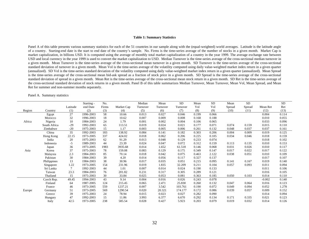
Table 1: Summary Statistics Panel A of this table presents various summary statistics for each of the 51 countries in our sample along with the (equal-weighted) world averages. Latitude is the latitude angle of a country. Starting-end date is the start to end date of the country’s sample. No. Firms is the time-series average of the number of stocks in a given month. Market Cap is market capitalization, in billions USD. It is computed using the average of monthly total market capitalization of a country in the year 1999. The average exchange rate between USD and local currency in the year 1999 is used to convert the market capitalization to USD. Median Turnover is the time-series average of the cross-sectional median turnover in a given month. Mean Turnover is the time-series average of the cross-sectional mean turnover in a given month. SD Turnover is the time-series average of the cross-sectional standard deviation of turnover in a given month. Mean Vol is the time-series average of the volatility computed using daily value-weighted market index return in a given quarter (annualized). SD Vol is the time-series standard deviation of the volatility computed using daily value-weighted market index return in a given quarter (annualized). Mean Spread is the time-series average of the cross-sectional mean bid-ask spread as a fraction of stock price in a given month. SD Spread is the time-series average of the cross-sectional standard deviation of spread in a given month. Mean Ret is the time-series average of the cross-sectional mean stock return in a given month. SD Ret is the time-series average of the cross-sectional standard deviation of stock returns in a given month. Panel B of this table summarizes Median Turnover, Mean Turnover, Mean Vol, Mean Spread, and Mean Ret for summer and non-summer months separately. Panel A. Summary statistics

Region Country Latitude

(1)

Starting - end Date

(2)

No. Firms

(3)

Market Cap

(4)

Median Turnover

(5)

Mean Turnover

(6)

SD Turnover

(7)

Mean Vol (8)

SD Vol (9)

Mean Spread

(10)

SD Spread

(11)

Mean Ret

(12)

SD Ret (13)

Africa

Egypt 27 1996-2003 58 10.66 0.013 0.027 0.046 0.199 0.066 0.004 0.114 Morocco 32 1996-2003 18 10.62 0.007 0.009 0.008 0.168 0.188 0.010 0.055 Nigeria 10 1984-2003 24 1.79 0.001 0.002 0.004 0.106 0.065 0.033 0.096

South Africa -29 1992-2003 65 113.51 0.019 0.024 0.021 0.177 0.071 0.074 0.159 0.015 0.110 Zimbabwe -20 1975-2003 15 1.17 0.003 0.005 0.006 0.261 0.132 0.048 0.037 0.037 0.161

Asia

China 35 1992-2003 183 138.92 0.084 0.141 0.182 0.303 0.206 0.004 0.009 0.019 0.125 Hong Kong 22.15 1973-2005 337 424.02 0.018 0.062 0.206 0.225 0.105 0.034 0.046 0.018 0.159

India 20 1975-2003 62 91.29 0.013 0.048 0.129 0.233 0.074 0.018 0.102 Indonesia -5 1989-2003 44 23.39 0.024 0.047 0.072 0.312 0.159 0.113 0.135 0.010 0.153

Japan 36 1973-2005 1983 3935.68 0.014 1.652 61.518 0.146 0.068 0.031 0.026 0.010 0.117 Korea 37 1975-2003 78 159.08 0.083 0.129 0.175 0.349 0.147 0.017 0.022 0.017 0.122

Malaysia 2.3 1984-2003 85 70.14 0.018 0.042 0.075 0.463 2.122 0.038 0.051 0.010 0.109 Pakistan 30 1984-2003 39 4.20 0.014 0.056 0.117 0.327 0.137 0.017 0.107

Philippines 13 1984-2003 38 30.96 0.017 0.035 0.051 0.215 0.095 0.141 0.167 0.019 0.140 Singapore 1.22 1973-2005 154 231.96 0.019 1.835 32.209 0.211 0.104 0.057 0.093 0.011 0.094 Sri Lanka 7 1992-2003 44 1.01 0.007 0.014 0.024 0.190 0.133 0.011 0.106 Taiwan 23.3 1984-2003 76 201.82 0.231 0.317 0.305 0.289 0.121 0.016 0.105

Thailand 15 1975-2003 30 33.84 0.025 0.053 0.081 0.363 0.185 0.050 0.103 0.014 0.110

Europe

Czech Rep. 49.45 1994-2003 43 9.14 0.004 0.016 0.026 0.243 0.078 -0.002 0.140 Finland 64 1987-2005 124 215.45 0.065 2.471 25.830 0.260 0.132 0.047 0.064 0.016 0.123 France 46 1973-2005 559 1237.21 0.007 3.542 103.761 0.190 0.072 0.049 0.094 0.052 1.278

Germany 51 1973-2005 569 1290.54 0.020 20.321 174.177 0.172 0.086 0.039 0.057 0.009 0.152 Greece 39 1975-2003 24 78.94 0.015 0.023 0.027 0.282 0.090 0.014 0.094

Hungary 47 1992-2003 15 11.86 3.993 6.377 6.670 0.292 0.134 0.171 0.335 0.021 0.123 Italy 42.5 1973-2005 238 585.54 0.028 0.427 5.923 0.203 0.079 0.019 0.032 0.014 0.126

32

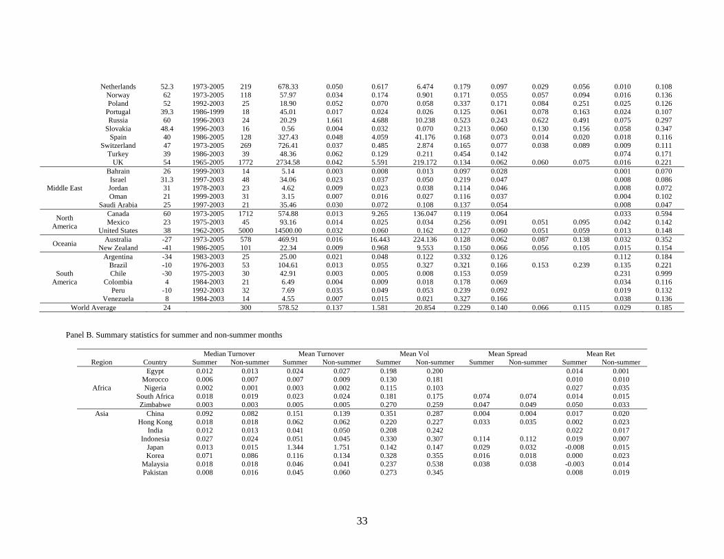
Netherlands 52.3 1973-2005 219 678.33 0.050 0.617 6.474 0.179 0.097 0.029 0.056 0.010 0.108 Norway 62 1973-2005 118 57.97 0.034 0.174 0.901 0.171 0.055 0.057 0.094 0.016 0.136 Poland 52 1992-2003 25 18.90 0.052 0.070 0.058 0.337 0.171 0.084 0.251 0.025 0.126

Portugal 39.3 1986-1999 18 45.01 0.017 0.024 0.026 0.125 0.061 0.078 0.163 0.024 0.107 Russia 60 1996-2003 24 20.29 1.661 4.688 10.238 0.523 0.243 0.622 0.491 0.075 0.297

Slovakia 48.4 1996-2003 16 0.56 0.004 0.032 0.070 0.213 0.060 0.130 0.156 0.058 0.347 Spain 40 1986-2005 128 327.43 0.048 4.059 41.176 0.168 0.073 0.014 0.020 0.018 0.116

Switzerland 47 1973-2005 269 726.41 0.037 0.485 2.874 0.165 0.077 0.038 0.089 0.009 0.111 Turkey 39 1986-2003 39 48.36 0.062 0.129 0.211 0.454 0.142 0.074 0.171

UK 54 1965-2005 1772 2734.58 0.042 5.591 219.172 0.134 0.062 0.060 0.075 0.016 0.221

Middle East

Bahrain 26 1999-2003 14 5.14 0.003 0.008 0.013 0.097 0.028 0.001 0.070 Israel 31.3 1997-2003 48 34.06 0.023 0.037 0.050 0.219 0.047 0.008 0.086 Jordan 31 1978-2003 23 4.62 0.009 0.023 0.038 0.114 0.046 0.008 0.072 Oman 21 1999-2003 31 3.15 0.007 0.016 0.027 0.116 0.037 0.004 0.102

Saudi Arabia 25 1997-2003 21 35.46 0.030 0.072 0.108 0.137 0.054 0.008 0.047

North America

Canada 60 1973-2005 1712 574.88 0.013 9.265 136.047 0.119 0.064 0.033 0.594 Mexico 23 1975-2003 45 93.16 0.014 0.025 0.034 0.256 0.091 0.051 0.095 0.042 0.142

United States 38 1962-2005 5000 14500.00 0.032 0.060 0.162 0.127 0.060 0.051 0.059 0.013 0.148

Oceania Australia -27 1973-2005 578 469.91 0.016 16.443 224.136 0.128 0.062 0.087 0.138 0.032 0.352 New Zealand -41 1986-2005 101 22.34 0.009 0.968 9.553 0.150 0.066 0.056 0.105 0.015 0.154

South America

Argentina -34 1983-2003 25 25.00 0.021 0.048 0.122 0.332 0.126 0.112 0.184 Brazil -10 1976-2003 53 104.61 0.013 0.055 0.327 0.321 0.166 0.153 0.239 0.135 0.221 Chile -30 1975-2003 30 42.91 0.003 0.005 0.008 0.153 0.059 0.231 0.999

Colombia 4 1984-2003 21 6.49 0.004 0.009 0.018 0.178 0.069 0.034 0.116 Peru -10 1992-2003 32 7.69 0.035 0.049 0.053 0.239 0.092 0.019 0.132

Venezuela 8 1984-2003 14 4.55 0.007 0.015 0.021 0.327 0.166 0.038 0.136 World Average 24 300 578.52 0.137 1.581 20.854 0.229 0.140 0.066 0.115 0.029 0.185

Panel B. Summary statistics for summer and non-summer months

Median Turnover Mean Turnover Mean Vol Mean Spread Mean Ret Region Country Summer Non-summer Summer Non-summer Summer Non-summer Summer Non-summer Summer Non-summer

Africa

Egypt 0.012 0.013 0.024 0.027 0.198 0.200 0.014 0.001 Morocco 0.006 0.007 0.007 0.009 0.130 0.181 0.010 0.010 Nigeria 0.002 0.001 0.003 0.002 0.115 0.103 0.027 0.035

South Africa 0.018 0.019 0.023 0.024 0.181 0.175 0.074 0.074 0.014 0.015 Zimbabwe 0.003 0.003 0.005 0.005 0.270 0.259 0.047 0.049 0.050 0.033

Asia

China 0.092 0.082 0.151 0.139 0.351 0.287 0.004 0.004 0.017 0.020 Hong Kong 0.018 0.018 0.062 0.062 0.220 0.227 0.033 0.035 0.002 0.023

India 0.012 0.013 0.041 0.050 0.208 0.242 0.022 0.017 Indonesia 0.027 0.024 0.051 0.045 0.330 0.307 0.114 0.112 0.019 0.007

Japan 0.013 0.015 1.344 1.751 0.142 0.147 0.029 0.032 -0.008 0.015 Korea 0.071 0.086 0.116 0.134 0.328 0.355 0.016 0.018 0.000 0.023

Malaysia 0.018 0.018 0.046 0.041 0.237 0.538 0.038 0.038 -0.003 0.014 Pakistan 0.008 0.016 0.045 0.060 0.273 0.345 0.008 0.019

33

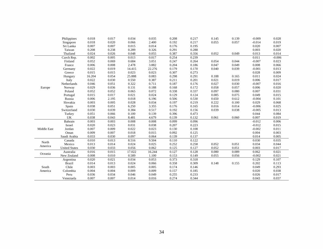
34

Philippines 0.018 0.017 0.034 0.035 0.208 0.217 0.145 0.139 -0.009 0.028 Singapore 0.018 0.020 0.066 2.400 0.192 0.217 0.055 0.057 -0.014 0.019 Sri Lanka 0.007 0.007 0.015 0.014 0.176 0.195 0.020 0.007 Taiwan 0.208 0.238 0.289 0.326 0.291 0.288 0.003 0.020

Thailand 0.024 0.026 0.048 0.055 0.387 0.356 0.052 0.049 0.013 0.014

Europe

Czech Rep. 0.002 0.005 0.013 0.017 0.254 0.239 0.011 -0.006 Finland 0.052 0.069 0.684 3.051 0.247 0.264 0.054 0.044 -0.007 0.023 France 0.006 0.008 2.478 3.882 0.204 0.186 0.047 0.049 0.008 0.066

Germany 0.022 0.019 14.415 22.276 0.179 0.170 0.040 0.039 -0.001 0.013 Greece 0.015 0.015 0.023 0.023 0.307 0.273 0.028 0.009

Hungary 16.204 0.054 25.888 0.083 0.298 0.291 0.188 0.165 0.011 0.024 Italy 0.022 0.030 0.550 0.387 0.211 0.201 0.021 0.019 0.006 0.017

Netherlands 0.046 0.051 0.322 0.711 0.187 0.176 0.027 0.030 -0.007 0.016 Norway 0.029 0.036 0.131 0.188 0.168 0.172 0.058 0.057 0.006 0.020 Poland 0.052 0.052 0.065 0.072 0.338 0.337 0.097 0.080 0.007 0.031

Portugal 0.015 0.017 0.021 0.024 0.129 0.124 0.085 0.075 0.049 0.015 Russia 0.006 2.195 0.018 6.196 0.506 0.530 0.650 0.612 -0.004 0.101

Slovakia 0.003 0.005 0.028 0.034 0.197 0.219 0.222 0.100 0.029 0.068 Spain 0.038 0.051 6.250 3.355 0.176 0.165 0.016 0.014 -0.006 0.025

Switzerland 0.030 0.039 0.384 0.517 0.192 0.156 0.039 0.038 -0.005 0.013 Turkey 0.051 0.066 0.100 0.139 0.396 0.473 0.044 0.084

UK 0.038 0.043 8.481 4.679 0.139 0.132 0.061 0.060 0.007 0.019

Middle East

Bahrain 0.003 0.003 0.008 0.008 0.099 0.096 -0.012 0.006 Israel 0.020 0.023 0.031 0.038 0.207 0.223 -0.012 0.015 Jordan 0.007 0.009 0.022 0.023 0.130 0.108 -0.002 0.011 Oman 0.009 0.007 0.018 0.015 0.092 0.125 0.004 0.003

Saudi Arabia 0.033 0.030 0.097 0.064 0.139 0.137 0.014 0.005

North America

Canada 0.010 0.013 8.516 9.504 0.110 0.122 0.030 0.035 Mexico 0.013 0.014 0.024 0.025 0.252 0.258 0.052 0.051 0.034 0.044

United States 0.030 0.033 0.056 0.062 0.125 0.127 0.052 0.051 0.003 0.017

Oceania Australia 0.016 0.015 17.022 16.244 0.127 0.128 0.080 0.089 0.062 0.021 New Zealand 0.008 0.010 0.589 1.100 0.153 0.149 0.055 0.056 -0.002 0.021

South America

Argentina 0.020 0.021 0.034 0.053 0.373 0.318 0.129 0.107 Brazil 0.014 0.013 0.024 0.066 0.358 0.309 0.148 0.155 0.202 0.113 Chile 0.003 0.003 0.005 0.005 0.174 0.146 0.049 0.293

Colombia 0.004 0.004 0.009 0.009 0.157 0.185 0.020 0.038 Peru 0.036 0.034 0.046 0.049 0.255 0.233 0.026 0.017

Venezuela 0.007 0.007 0.014 0.016 0.274 0.344 0.043 0.037

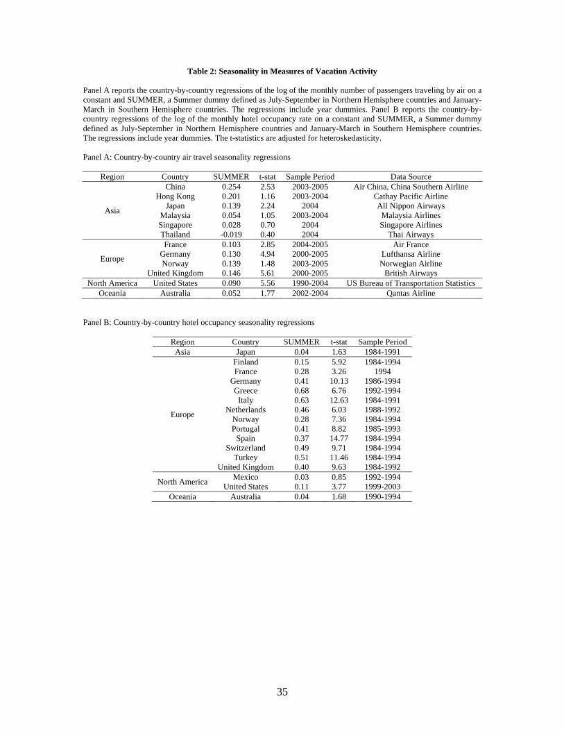
Table 2: Seasonality in Measures of Vacation Activity Panel A reports the country-by-country regressions of the log of the monthly number of passengers traveling by air on a constant and SUMMER, a Summer dummy defined as July-September in Northern Hemisphere countries and January-March in Southern Hemisphere countries. The regressions include year dummies. Panel B reports the country-by-country regressions of the log of the monthly hotel occupancy rate on a constant and SUMMER, a Summer dummy defined as July-September in Northern Hemisphere countries and January-March in Southern Hemisphere countries. The regressions include year dummies. The t-statistics are adjusted for heteroskedasticity. Panel A: Country-by-country air travel seasonality regressions

Region Country SUMMER t-stat Sample Period Data Source

Asia

China 0.254 2.53 2003-2005 Air China, China Southern Airline Hong Kong 0.201 1.16 2003-2004 Cathay Pacific Airline

Japan 0.139 2.24 2004 All Nippon Airways Malaysia 0.054 1.05 2003-2004 Malaysia Airlines Singapore 0.028 0.70 2004 Singapore Airlines Thailand -0.019 0.40 2004 Thai Airways

Europe

France 0.103 2.85 2004-2005 Air France Germany 0.130 4.94 2000-2005 Lufthansa Airline Norway 0.139 1.48 2003-2005 Norwegian Airline

United Kingdom 0.146 5.61 2000-2005 British Airways North America United States 0.090 5.56 1990-2004 US Bureau of Transportation Statistics

Oceania Australia 0.052 1.77 2002-2004 Qantas Airline Panel B: Country-by-country hotel occupancy seasonality regressions

Region Country SUMMER t-stat Sample Period Asia Japan 0.04 1.63 1984-1991

Europe

Finland 0.15 5.92 1984-1994 France 0.28 3.26 1994

Germany 0.41 10.13 1986-1994 Greece 0.68 6.76 1992-1994

Italy 0.63 12.63 1984-1991 Netherlands 0.46 6.03 1988-1992

Norway 0.28 7.36 1984-1994 Portugal 0.41 8.82 1985-1993

Spain 0.37 14.77 1984-1994 Switzerland 0.49 9.71 1984-1994

Turkey 0.51 11.46 1984-1994 United Kingdom 0.40 9.63 1984-1992

North America Mexico 0.03 0.85 1992-1994 United States 0.11 3.77 1999-2003

Oceania Australia 0.04 1.68 1990-1994

35

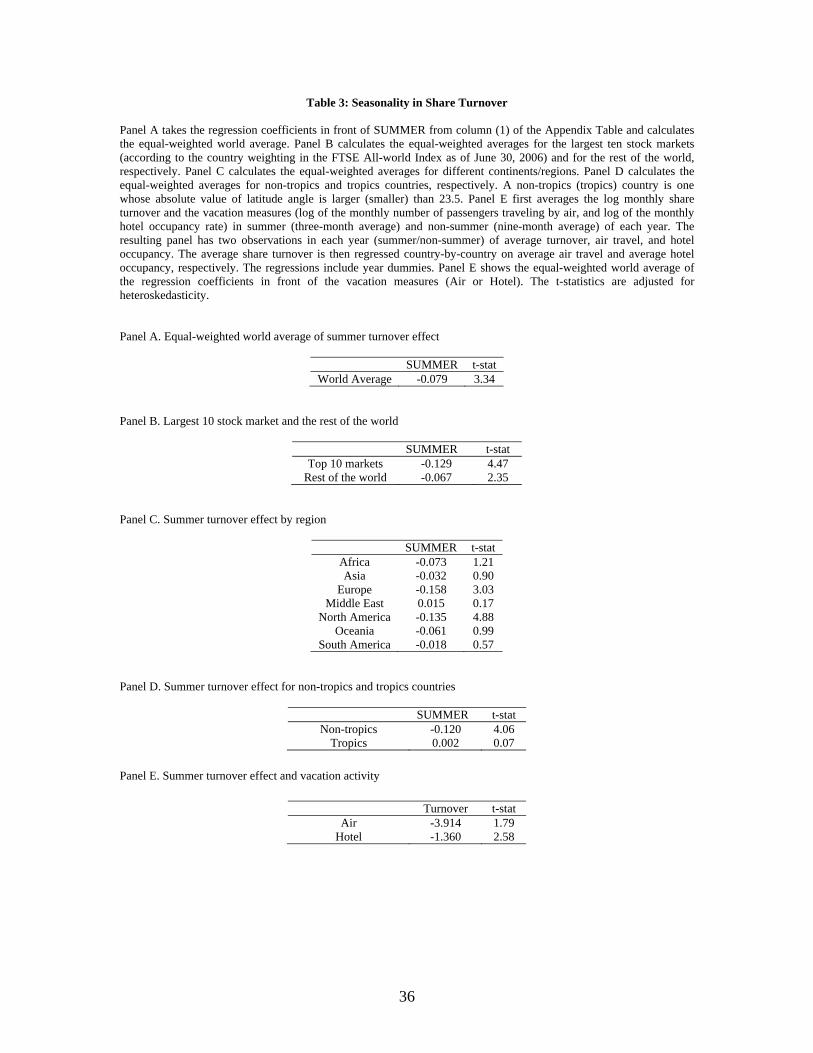
Table 3: Seasonality in Share Turnover Panel A takes the regression coefficients in front of SUMMER from column (1) of the Appendix Table and calculates the equal-weighted world average. Panel B calculates the equal-weighted averages for the largest ten stock markets (according to the country weighting in the FTSE All-world Index as of June 30, 2006) and for the rest of the world, respectively. Panel C calculates the equal-weighted averages for different continents/regions. Panel D calculates the equal-weighted averages for non-tropics and tropics countries, respectively. A non-tropics (tropics) country is one whose absolute value of latitude angle is larger (smaller) than 23.5. Panel E first averages the log monthly share turnover and the vacation measures (log of the monthly number of passengers traveling by air, and log of the monthly hotel occupancy rate) in summer (three-month average) and non-summer (nine-month average) of each year. The resulting panel has two observations in each year (summer/non-summer) of average turnover, air travel, and hotel occupancy. The average share turnover is then regressed country-by-country on average air travel and average hotel occupancy, respectively. The regressions include year dummies. Panel E shows the equal-weighted world average of the regression coefficients in front of the vacation measures (Air or Hotel). The t-statistics are adjusted for heteroskedasticity.

Panel A. Equal-weighted world average of summer turnover effect

SUMMER t-stat World Average -0.079 3.34

Panel B. Largest 10 stock market and the rest of the world

SUMMER t-stat Top 10 markets -0.129 4.47

Rest of the world -0.067 2.35 Panel C. Summer turnover effect by region

SUMMER t-stat Africa -0.073 1.21 Asia -0.032 0.90

Europe -0.158 3.03 Middle East 0.015 0.17

North America -0.135 4.88 Oceania -0.061 0.99

South America -0.018 0.57 Panel D. Summer turnover effect for non-tropics and tropics countries

SUMMER t-stat Non-tropics -0.120 4.06

Tropics 0.002 0.07

Panel E. Summer turnover effect and vacation activity

Turnover t-stat Air -3.914 1.79

Hotel -1.360 2.58

36

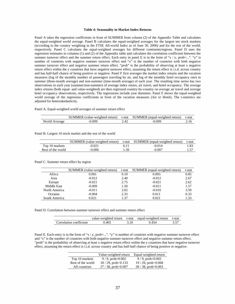
Table 4: Seasonality in Market Index Returns Panel A takes the regression coefficients in front of SUMMER from column (2) of the Appendix Table and calculates the equal-weighted world average. Panel B calculates the equal-weighted averages for the largest ten stock markets (according to the country weighting in the FTSE All-world Index as of June 30, 2006) and for the rest of the world, respectively. Panel C calculates the equal-weighted averages for different continents/regions. Panel D uses the regression estimates in columns (1) and (2) of the Appendix table and calculates the correlation coefficient between the summer turnover effect and the summer return effect. Each entry in panel E is in the form of “x / y, prob=...”. “y” is number of countries with negative summer turnover effect and “x” is the number of countries with both negative summer turnover effect and negative summer return effect. “prob” is the probability of observing at least x negative return effect within the y countries that have negative turnover effect, assuming the return effect is i.i.d. across country and has half-half chance of being positive or negative. Panel F first averages the market index returns and the vacation measures (log of the monthly number of passengers traveling by air, and log of the monthly hotel occupancy rate) in summer (three-month average) and non-summer (nine-month average) of each year. The resulting time series has two observations in each year (summer/non-summer) of average index return, air travel, and hotel occupancy. The average index returns (both equal- and value-weighted) are then regressed country-by-country on average air travel and average hotel occupancy observations, respectively. The regressions include year dummies. Panel F shows the equal-weighted world average of the regression coefficients in front of the vacation measures (Air or Hotel). The t-statistics are adjusted for heteroskedasticity.

Panel A. Equal-weighted world averages of summer return effect

SUMMER (value-weighted return) t-stat SUMMER (equal-weighted return) t-stat World Average -0.009 2.42 -0.009 2.16

Panel B. Largest 10 stock market and the rest of the world

SUMMER (value-weighted return) t-stat SUMMER (equal-weighted return) t-stat Top 10 markets -0.021 6.11 -0.014 1.83

Rest of the world -0.006 1.39 -0.007 1.57 Panel C. Summer return effect by region

SUMMER (value-weighted return) t-stat SUMMER (equal-weighted return) t-stat Africa 0.001 0.19 0.003 0.85 Asia -0.012 2.40 -0.012 2.67

Europe -0.021 2.75 -0.021 2.62 Middle East -0.009 1.50 -0.011 1.57

North America -0.011 3.02 -0.010 3.59 Oceania -0.004 2.33 0.011 0.33

South America 0.021 1.37 0.021 1.33

Panel D. Correlation between summer turnover effect and summer return effect

value-weighted return t-stat equal-weighted return t-stat Correlation coefficient 0.405 3.10 0.454 3.57

Panel E. Each entry is in the form of “x / y, prob=...”. “y” is number of countries with negative summer turnover effect and “x” is the number of countries with both negative summer turnover effect and negative summer return effect. “prob” is the probability of observing at least x negative return effect within the y countries that have negative turnover effect, assuming the return effect is i.i.d. across country and has half-half chance of being positive or negative.

Value-weighted return Equal-weighted return Top 10 markets 9 / 9, prob=0.002 9 / 9, prob=0.002

Rest of the world 18 / 29, prob=0.133 19 / 29, prob=0.068 All countries 27 / 38, prob=0.007 28 / 38, prob=0.003

37

Panel F. Summer return effect and vacation activity

Value-weighted return t-stat Equal-weighted return t-stat Air -0.083 0.91 -0.529 1.01

Hotel -0.126 1.08 -0.084 1.87

38

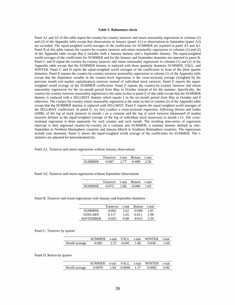
Table 5: Robustness check

Panel A1 and A2 of this table repeat the country-by-country turnover and return seasonality regressions in columns (1) and (2) of the Appendix table except that observations in January (panel A1) or observations in September (panel A2) are excluded. The equal-weighted world averages of the coefficients for SUMMER are reported in panel A1 and A2. Panel B of this table repeats the country-by-country turnover and return seasonality regressions in columns (1) and (2) of the Appendix table except that it includes both a January dummy and a September dummy. The equal-weighted world averages of the coefficients for SUMMER and for the January and September dummies are reported in panel B. Panel C and D repeat the country-by-country turnover and return seasonality regressions in columns (1) and (2) of the Appendix table except that the SUMMER dummy is replaced with three quarterly dummies SUMMER, FALL, and WINTER. Panel C and D report the equal-weighted world averages of the coefficients in front of the three quarter dummies. Panel E repeats the country-by-country turnover seasonality regressions in column (1) of the Appendix table except that the dependent variable in the country-level regressions is the cross-sectional average (weighted by the previous month end market capitalization) turnover instead of individual stock turnover. Panel E reports the equal-weighted world average of the SUMMER coefficients. Panel F repeats the country-by-country turnover and return seasonality regressions for the six-month period from May to October instead of for the summer. Specifically, the country-by-country turnover seasonality regression is the same as that in panel E of this table except that the SUMMER dummy is replaced with a SELLMAY dummy which equals 1 in the six-month period from May to October and 0 otherwise. The country-by-country return seasonality regression is the same as that in column (2) of the Appendix table except that the SUMMER dummy is replaced with SELLMAY. Panel F reports the equal-weighted world averages of the SELLMAY coefficients. In panel G, we first conduct a cross-sectional regression, following Heston and Sadka (2008), of the log of stock turnover in month t on a constant and the log of stock turnover (demeaned of market turnover defined as the equal-weighted average of the log of individual stock turnovers) in month t-12. The cross-sectional regression is done separately for each country and each month. The resulting time-series of regression intercept is then regressed country-by-country on a constant and SUMMER, a summer dummy defined as July-September in Northern Hemisphere countries and January-March in Southern Hemisphere countries. The regressions include year dummies. Panel G shows the equal-weighted world average of the coefficients for SUMMER. The t-statistics are adjusted for heteroskedasticity. Panel A1. Turnover and return regressions without January observations

Turnover t-stat Return t-stat SUMMER -0.067 2.77 -0.009 2.56

Panel A2. Turnover and return regressions without September observations

Turnover t-stat Return t-stat SUMMER -0.075 2.86 -0.006 1.69

Panel B. Turnover and return regressions with January and September dummies

Turnover t-stat Return t-stat SUMMER -0.062 2.62 -0.006 1.81 JANUARY 0.117 1.65 0.011 1.98

SEPTEMBER -0.025 0.88 -0.015 3.29 Panel C. Turnover by quarter

SUMMER t-stat FALL t-stat WINTER t-stat World average -0.081 2.37 -0.041 1.06 0.036 1.04

Panel D. Return by quarter

SUMMER t-stat FALL t-stat WINTER t-stat World average -0.0076 1.94 0.0048 1.37 0.0002 0.06

39

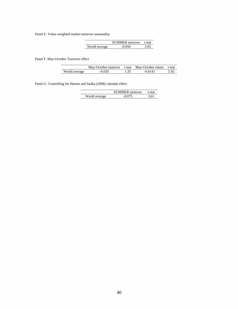
Panel E. Value-weighted market turnover seasonality

SUMMER turnover t-stat World average -0.059 3.93

Panel F. May-October Turnover effect

May-October turnover t-stat May-October return t-stat World average -0.020 1.35 -0.0141 5.92

Panel G. Controlling for Heston and Sadka (2008) calendar effect

SUMMER turnover t-stat

World average -0.075 3.61

40

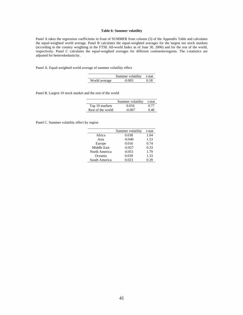
Table 6: Summer volatility Panel A takes the regression coefficients in front of SUMMER from column (3) of the Appendix Table and calculates the equal-weighted world average. Panel B calculates the equal-weighted averages for the largest ten stock markets (according to the country weighting in the FTSE All-world Index as of June 30, 2006) and for the rest of the world, respectively. Panel C calculates the equal-weighted averages for different continents/regions. The t-statistics are adjusted for heteroskedasticity. Panel A. Equal-weighted world average of summer volatility effect

Summer volatility t-stat World average -0.003 0.18

Panel B. Largest 10 stock market and the rest of the world

Summer volatility t-stat Top 10 markets 0.016 0.77

Rest of the world -0.007 0.40

Panel C. Summer volatility effect by region

Summer volatility t-stat Africa 0.038 1.04 Asia -0.040 1.53

Europe 0.016 0.74 Middle East -0.027 0.33

North America -0.051 1.79 Oceania 0.039 1.33

South America 0.023 0.39

41

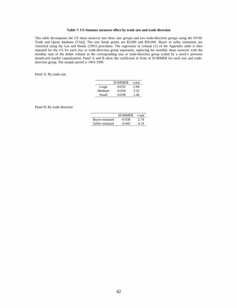
Table 7: US Summer turnover effect by trade size and trade direction This table decomposes the US share turnover into three size groups and two trade-direction groups using the NYSE Trade and Quote database (TAQ). The size break points are $5,000 and $50,000. Buyer or seller initiations are classified using the Lee and Ready (1991) procedure. The regression in column (1) of the Appendix table is then repeated for the US for each size or trade-direction group separately, replacing the monthly share turnover with the monthly sum of the dollar volume in the corresponding size or trade-direction group scaled by a stock’s previous month-end market capitalization. Panel A and B show the coefficient in front of SUMMER for each size and trade-direction group. The sample period is 1993-1999. Panel A. By trade size

SUMMER t-stat Large -0.032 2.69

Medium -0.034 3.52 Small -0.038 2.46

Panel B. By trade direction

SUMMER t-stat Buyer-initiated -0.038 2.74 Seller-initiated -0.045 4.19

42

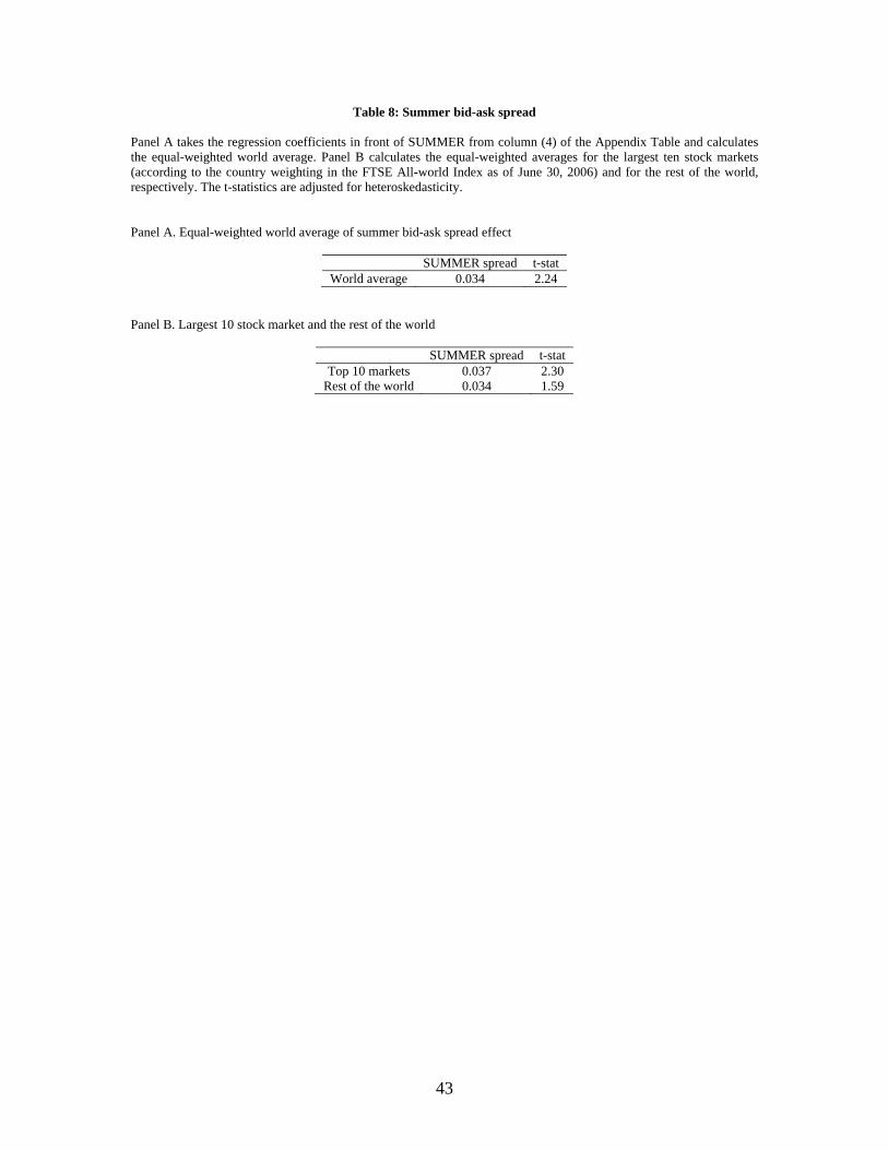
Table 8: Summer bid-ask spread Panel A takes the regression coefficients in front of SUMMER from column (4) of the Appendix Table and calculates the equal-weighted world average. Panel B calculates the equal-weighted averages for the largest ten stock markets (according to the country weighting in the FTSE All-world Index as of June 30, 2006) and for the rest of the world, respectively. The t-statistics are adjusted for heteroskedasticity. Panel A. Equal-weighted world average of summer bid-ask spread effect

SUMMER spread t-stat World average 0.034 2.24

Panel B. Largest 10 stock market and the rest of the world

SUMMER spread t-stat Top 10 markets 0.037 2.30

Rest of the world 0.034 1.59

43

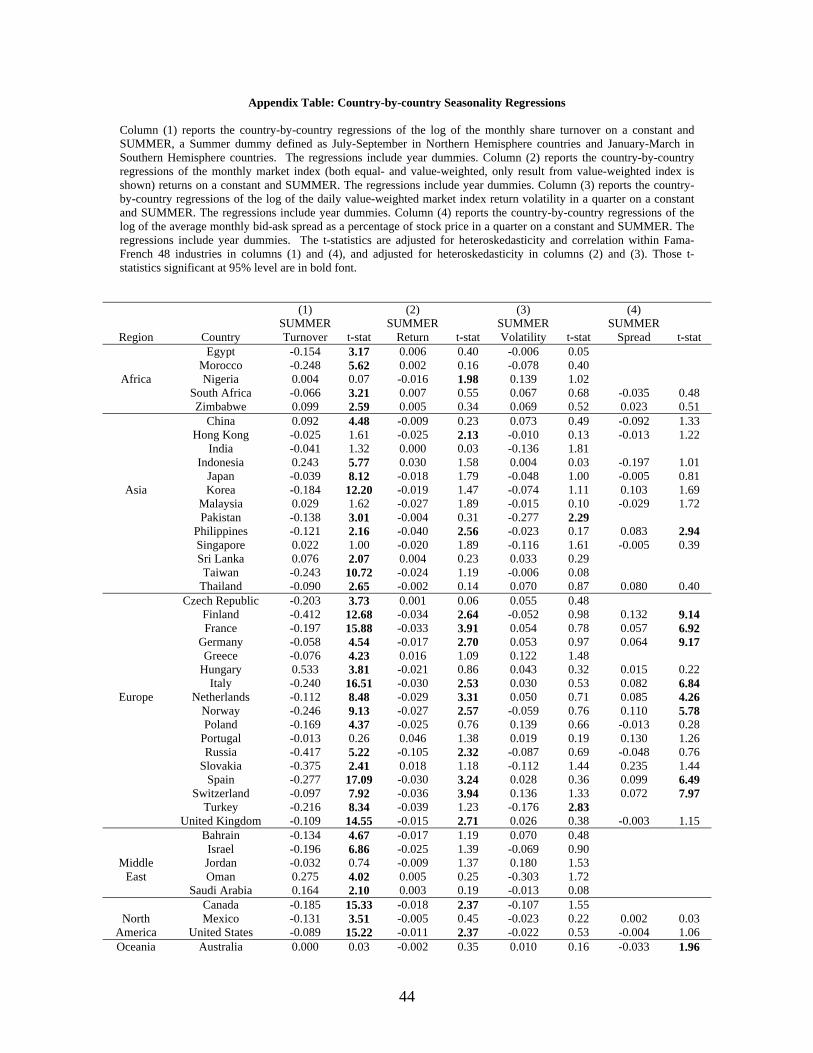
Appendix Table: Country-by-country Seasonality Regressions Column (1) reports the country-by-country regressions of the log of the monthly share turnover on a constant and SUMMER, a Summer dummy defined as July-September in Northern Hemisphere countries and January-March in Southern Hemisphere countries. The regressions include year dummies. Column (2) reports the country-by-country regressions of the monthly market index (both equal- and value-weighted, only result from value-weighted index is shown) returns on a constant and SUMMER. The regressions include year dummies. Column (3) reports the country-by-country regressions of the log of the daily value-weighted market index return volatility in a quarter on a constant and SUMMER. The regressions include year dummies. Column (4) reports the country-by-country regressions of the log of the average monthly bid-ask spread as a percentage of stock price in a quarter on a constant and SUMMER. The regressions include year dummies. The t-statistics are adjusted for heteroskedasticity and correlation within Fama-French 48 industries in columns (1) and (4), and adjusted for heteroskedasticity in columns (2) and (3). Those t-statistics significant at 95% level are in bold font.

Region Country

(1) SUMMER Turnover t-stat

(2) SUMMER

Return t-stat

(3) SUMMER Volatility t-stat

(4) SUMMER

Spread t-stat

Africa

Egypt -0.154 3.17 0.006 0.40 -0.006 0.05 Morocco -0.248 5.62 0.002 0.16 -0.078 0.40 Nigeria 0.004 0.07 -0.016 1.98 0.139 1.02

South Africa -0.066 3.21 0.007 0.55 0.067 0.68 -0.035 0.48 Zimbabwe 0.099 2.59 0.005 0.34 0.069 0.52 0.023 0.51

Asia

China 0.092 4.48 -0.009 0.23 0.073 0.49 -0.092 1.33 Hong Kong -0.025 1.61 -0.025 2.13 -0.010 0.13 -0.013 1.22

India -0.041 1.32 0.000 0.03 -0.136 1.81 Indonesia 0.243 5.77 0.030 1.58 0.004 0.03 -0.197 1.01

Japan -0.039 8.12 -0.018 1.79 -0.048 1.00 -0.005 0.81 Korea -0.184 12.20 -0.019 1.47 -0.074 1.11 0.103 1.69

Malaysia 0.029 1.62 -0.027 1.89 -0.015 0.10 -0.029 1.72 Pakistan -0.138 3.01 -0.004 0.31 -0.277 2.29

Philippines -0.121 2.16 -0.040 2.56 -0.023 0.17 0.083 2.94 Singapore 0.022 1.00 -0.020 1.89 -0.116 1.61 -0.005 0.39 Sri Lanka 0.076 2.07 0.004 0.23 0.033 0.29 Taiwan -0.243 10.72 -0.024 1.19 -0.006 0.08

Thailand -0.090 2.65 -0.002 0.14 0.070 0.87 0.080 0.40

Europe

Czech Republic -0.203 3.73 0.001 0.06 0.055 0.48 Finland -0.412 12.68 -0.034 2.64 -0.052 0.98 0.132 9.14 France -0.197 15.88 -0.033 3.91 0.054 0.78 0.057 6.92

Germany -0.058 4.54 -0.017 2.70 0.053 0.97 0.064 9.17 Greece -0.076 4.23 0.016 1.09 0.122 1.48

Hungary 0.533 3.81 -0.021 0.86 0.043 0.32 0.015 0.22 Italy -0.240 16.51 -0.030 2.53 0.030 0.53 0.082 6.84

Netherlands -0.112 8.48 -0.029 3.31 0.050 0.71 0.085 4.26 Norway -0.246 9.13 -0.027 2.57 -0.059 0.76 0.110 5.78 Poland -0.169 4.37 -0.025 0.76 0.139 0.66 -0.013 0.28

Portugal -0.013 0.26 0.046 1.38 0.019 0.19 0.130 1.26 Russia -0.417 5.22 -0.105 2.32 -0.087 0.69 -0.048 0.76

Slovakia -0.375 2.41 0.018 1.18 -0.112 1.44 0.235 1.44 Spain -0.277 17.09 -0.030 3.24 0.028 0.36 0.099 6.49

Switzerland -0.097 7.92 -0.036 3.94 0.136 1.33 0.072 7.97 Turkey -0.216 8.34 -0.039 1.23 -0.176 2.83

United Kingdom -0.109 14.55 -0.015 2.71 0.026 0.38 -0.003 1.15

Middle East

Bahrain -0.134 4.67 -0.017 1.19 0.070 0.48 Israel -0.196 6.86 -0.025 1.39 -0.069 0.90 Jordan -0.032 0.74 -0.009 1.37 0.180 1.53 Oman 0.275 4.02 0.005 0.25 -0.303 1.72

Saudi Arabia 0.164 2.10 0.003 0.19 -0.013 0.08

North America

Canada -0.185 15.33 -0.018 2.37 -0.107 1.55 Mexico -0.131 3.51 -0.005 0.45 -0.023 0.22 0.002 0.03

United States -0.089 15.22 -0.011 2.37 -0.022 0.53 -0.004 1.06 Oceania Australia 0.000 0.03 -0.002 0.35 0.010 0.16 -0.033 1.96

44

New Zealand -0.122 6.15 -0.005 0.60 0.068 0.91 -0.017 1.05

South America

Argentina -0.009 0.25 0.028 0.49 0.173 1.51 Brazil 0.039 1.83 0.090 2.01 0.120 0.65 0.156 1.75 Chile -0.039 1.20 0.018 1.26 0.124 1.18

Colombia -0.114 1.90 -0.019 1.75 -0.128 1.43 Peru 0.093 2.37 0.009 0.54 0.036 0.28

Venezuela -0.077 2.14 0.000 0.01 -0.184 2.48

45

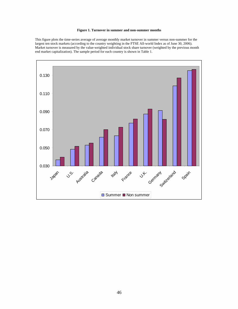
Figure 1. Turnover in summer and non-summer months

This figure plots the time-series average of average monthly market turnover in summer versus non-summer for the largest ten stock markets (according to the country weighting in the FTSE All-world Index as of June 30, 2006). Market turnover is measured by the value-weighted individual stock share turnover (weighted by the previous month end market capitalization). The sample period for each country is shown in Table 1.

0.030

0.050

0.070

0.090

0.110

0.130

Japa

nU.S.

Austra

lia

Canada Ita

ly

France

U.K.

German

y

Switzerl

andSpa

in

Summer Non summer

46