GLOBAL WARMING & CLIMATE SCIENCE

JOOP VAREKAMP, E&ES

Structure of this presentation

1. Global warming-real or not?2. Climate science, models and predictions the zero dimensional approach 3. Unexpected events

Is there evidence for Modern Global Warming?A. Instrumental recordsB. ‘Proxy’ records from the recent pastC. Current Environmental Change (glaciers,floral/faunal shifts)

How does MGW fit into the climate history of the recent geological past?

Source: OSTP

Source: IPCC TAR 2001

Variations of the Variations of the Earth’s Surface Earth’s Surface Temperature*Temperature*

*relative to 1961-1990 average*relative to 1961-1990 average

20001900180017001600150014001300120011001000900-34.50

-34.25

-34.00

-33.75

-33.50

Age Years AD

d18O

WARM

COLD

MWP LIA MGW

Superposed on gradual climate change, there is evidence for very sudden climate change from the

record of the past

U.S. Temperature Trends: 1901 to 1998U.S. Temperature Trends: 1901 to 1998

Red circles = warmingRed circles = warming; ; Blue circles = coolingBlue circles = coolingAll stations/trends displayed regardless of statistical significance.All stations/trends displayed regardless of statistical significance.

Source: National Climatic Data Center/NESDIS/NOAA

Crawford Ranch

Snow cover and ice extent have decreasedSnow cover and ice extent have decreased

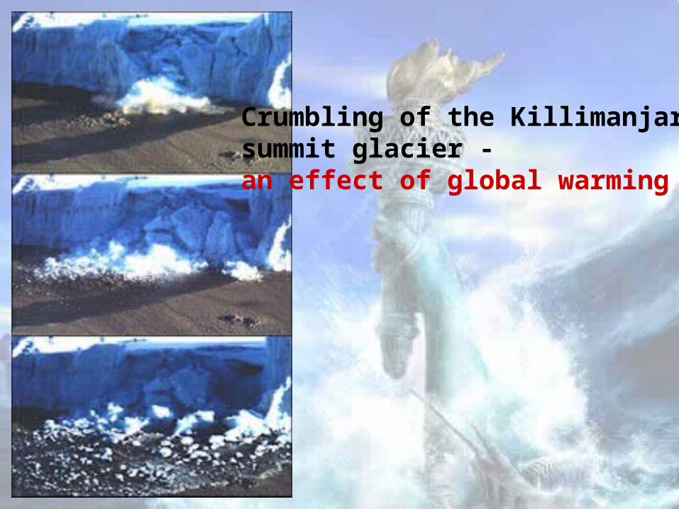
Crumbling of the Killimanjaro summit glacier - an effect of global warming

Collapse of the Larsen Ice Shelf near Antarctica - a piece of ice the size of Rhode Island came adrift

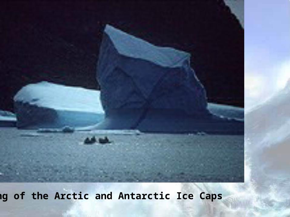
Melting of the Arctic and Antarctic Ice Caps

Global warmingGlobal warming(temperature increase)(temperature increase)

Effects of global warming on water cycleEffects of global warming on water cycle

Speeds up globalSpeeds up globalwater cyclewater cycle

More extreme weather eventsMore extreme weather events• DroughtsDroughts• StormsStorms• FloodsFloods

Increase in catastrophic flood eventsIncrease in catastrophic flood events

Increase in frequency and Increase in frequency and intensity of droughtsintensity of droughts

Source: OSTP

Extreme Precipitation Events in the U.S.Extreme Precipitation Events in the U.S.

Source: Karl, et.al. 1996.

So these are the data:There is global warming, there are

more extreme events, ice is melting, glaciers are retreating, rainfall

patterns are changing, plants and animal species are “moving”, sea

level is rising.

The real BIG question is:Natural Variability or the “Human Hand”?

The main “Radiation Law is Planck’s Law. Boltzman’s Law is the ‘integrated

version’ of PL

The HumanHand?!

GLOBAL WARMING IS LIKELY RELATED TO THE GREENHOUSE

EFFECT - HOW DOES THAT WORK?

FIRST WE SHOULD LOOK AT THE BASICS OF CLIMATE SCIENCE

Principle of Radiative Balance:The solid earth + atmosphere receive

heat from the sun BUTalso radiate the same amount of heat

back into space

Principles of terrestrial climate:

Incoming solar radiation equals outgoing terrestrial radiation

Rsun = Rterr The magnitude of Rterr depends on Ts (apply Boltzman Law).

Part of the outgoing terrestrial radiation is blocked by ‘greenhouse gases’, and the earth warms up a bit to restore the radiative equilibrium

Illumination of the earth by the sun:1. More heat received at the equator than at the poles2. Solid earth receives more heat by radiation than it radiates backRESULT: CONVECTIVE HEAT TRANSPORT FROM EQUATOR TO POLES THROUGH AIR AND OCEANS

The earth radiates long wavelength EMR which is

absorbed by molecules with an uneven # of atoms, such as H2O, CO2, CH4, CFC’s O3

(the “greenhouse” gases)

THE GREENHOUSE EFFECTTHE SUN EMITS SHORT WAVELENGTH RADIATION (‘VISIBLE LIGHT’) WHICH

PENETRATES THROUGH THE ATMOSPHERE AND HEATS THE SOLID EARTH.

THE SOLID EARTH EMITS LONG WAVE LENGTH RADIATION (‘INFRA RED’) WHICH

IS ABSORBED ‘ON ITS WAY OUT’ BY THE GREENHOUSE GASES.

A THERMAL BLANKET IS THE RESULT

THE TRACE GASES (H2O, CO2, CH4, N2O, O3) SERVE AS GREENHOUSE GASES AND

KEEP THE EARTH LIVABLE

IF THE GREENHOUSE EFFECT IS CHANGING:

CAN WE DOCUMENT CHANGES IN THE CHEMICAL COMPOSITION OF THE ATMOSPHERE?

COULD THESE BE ANTHROPOGENIC?

IS THEIR MAGNITUDE ENOUGH TO EXPLAIN MODERN GLOBAL WARMING?

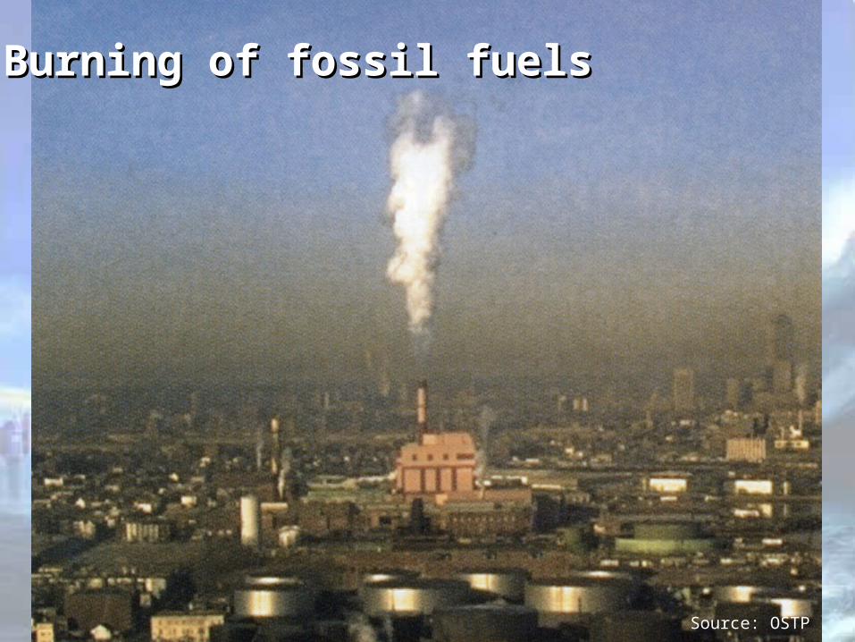
Burning of fossil fuelsBurning of fossil fuels

Source: OSTP

DeforestationDeforestation

Source: OSTP

Indicators of the Human InfluenceIndicators of the Human Influenceon the Atmosphere during the Industrial Eraon the Atmosphere during the Industrial Era

Source: IPCC TAR 2001

Source: OSTP

CARBON RESIDES IN AND MOVES BETWEEN DIFFERENT RESERVOIRS SUCH AS THE ATMOSPHERE, THE PLANT AND ANIMAL WORLD (BIOSPHERE), DISSOLVED IN THE OCEAN AND IN SOILS. THE CARBON MOVEMENTS BETWEEN THESE RESERVOIRS IS CALLED THE CARBON CYCLE

ANTHROPOGENIC CARBON FLUXES IN THE 1990s:

FOSSIL FUEL BURNING: 6 BILLION TONS CARBON/YEAR

DEFORESTATION: 1.1 BILLION TONS CARBON/YEAR

TOTAL: 7.1 BILLION TONS CARBON/YEAR

WHERE IS ALL THAT CO2 GOING??

How do we model future atmospheric CO2 concentrations?

• Apply a carbon cycle model to a range of future FFF scenarios

• Use ‘economic scenarios’ that depend strongly on

1. Population growth rates

2. Economic development

3. Switch to alternative energy technologies

4. Sharing of technology with the developing world

Carbon cycle model from E&ES 132/359 at Wesleyan University

Symbols:Mx = mass of carbonKx = rate constantFFF = Fossil Fuel Flux of Carbon

Feedbacks:Bf = Bioforcing factor; depends on CO2(atm)K4 = f(temperature)

200

300

400

500

600

700

800

900

1000

1100

1200

1850 1900 1950 2000 2050 2100Age

CO2 (atm) ppm

YOHE1

YOHE7

SRESA1

SRESA2

SRESB1

PRESENT FUTURE

THE E&ES 132/359 CARBON CYCLE MODEL

COCO22 and SO and SO22 in the 21 in the 21stst Century Century

Source: IPCC TAR 2001

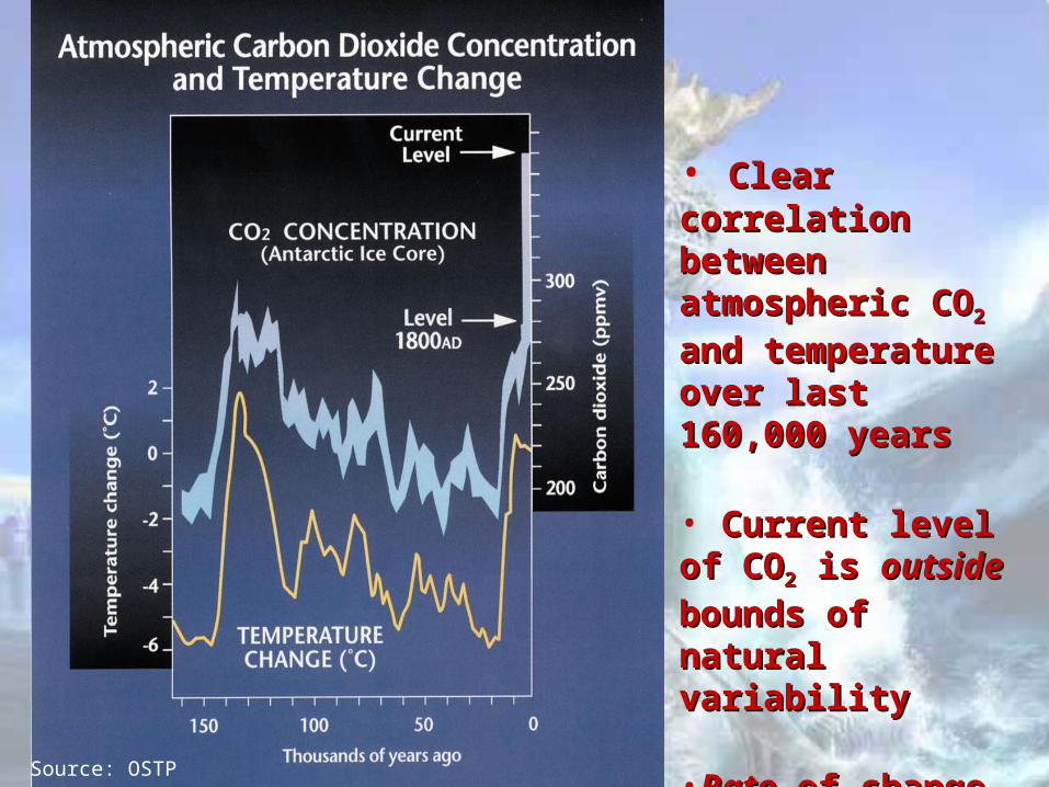
• Clear correlation Clear correlation between atmospheric between atmospheric COCO22 and temperature and temperature

over last 160,000 yearsover last 160,000 years

• Current level of COCurrent level of CO22

is is outsideoutside bounds of bounds of natural variabilitynatural variability

•RateRate of change of CO of change of CO22

is also unprecedentedis also unprecedented

Source: OSTP

If nothing is done to slow If nothing is done to slow greenhouse gas emissions. . .greenhouse gas emissions. . .

• COCO22 concentrations will likely be concentrations will likely be

more than 700 ppm by 2100 more than 700 ppm by 2100

•THIS IS WELL OUTSIDE THETHIS IS WELL OUTSIDE THE ‘ ‘NATURAL RANGE’ OF THENATURAL RANGE’ OF THE LAST 200,000 YEARSLAST 200,000 YEARS

2100

Source: OSTP

To go from atmospheric CO2 concentration change to climate change, we need to know the climate sensitivity parameter, .

The common approach is: Ts = ForF/Ts = 1/ where

F is the ‘radiative forcing’ caused by the increased CO2 concentration. The value of F can be calculated from the increase in CO2 concentration using the deBeers law.

Ts is the change in the surface temperature of the earth

We can solve for by taking the first derivative of Boltzman’s LawF = Ts

4 or dF/dTs = 4F/Ts leading to a value of 0.3 K/Wm-2.

This approach is the most fundamental response function and uses zero climate feedbacks! Most climate modellers use 0.5 K/Wm-2, incorporating various positive and negative feedbacks.

0.0

0.5

1.0

1.5

2.0

2.5

3.0

1850 1900 1950 2000 2050 2100AGE

delta T oC

YOHE 1

YOHE7

SRESA1

SRESA2

SRESB1

PRESENT FUTURE

THE E&ES 132/359 CLIMATE MODEL

• Global average temperature is projected to increase by 1.5 to 5.8 °C from 1990 to 2100

• Projected temperature increases are greater than those in the SAR (1.0 to 3.5 °C)

• Projected rate of warming is unprecedented for last 10,000 years

Temperature ProjectionsTemperature Projections

Source: IPCC TAR 2001

CONCLUSIONS:• Global warming is here! Its

effects have been documented extensively worldwide

• The human hand is, according to many, very visible

• Projections for the future are riddled with uncertainties, but all show further warming

• Largest source of uncertainty are the economic scenarios.

A recent movie suggested that global warming maylead to the early arrival

of the next Ice Age?

or

Could these be related?

WHICH OF THESE

SYMBOLS WILL BE

THE STRONGER

ONE??

CONCLUSIONS (2):• Natural climate variability over the

last 700,000 years is finely in tune with planetary motions-Ice ages do not occur at random!

• Superposed there are sudden climate changes (e.g., Younger Dryas) that have other origins (e.g., shut down of oceanic conveyor)

• As such, global warming can lead to sudden arrival of a new cold period (but over decades, not hours!)