GEOGRAPHIC PROFILING: BAYESIAN MODELS FOR …kolacek/docs/English1.pdf · GEOGRAPHIC PROFILING:...

GEOGRAPHIC PROFILING: BAYESIAN MODELS FOR RESIDENTS ANDNON-RESIDENTS

Keywords: Bayesian data analysis; geographic profiling; distance decay function;anchor point; resident; non-resident.

1

2

ABSTRACT. We consider the problem of geographic profiling and offer an ap-proach to choosing a suitable model for each offender. Based on the analysis ofthe examined dataset, we divide offenders into several types with similar behav-ior. According to the spatial distribution of the offender’s crime sites, each newcriminal is assigned to the corresponding group. Then we choose an appropriatemodel for the offender and using bayesian methods we determine the posteriordistribution for the criminal’s anchor point. Our models include directionality,similarly to models of Mohler and Short (2012). Our approach also provides away to incorporate two possible situations into the model – when the criminalis resident or non-resident. We test this methodology on a data set of offendersfrom Baltimore County and compare the results with Rossmo’s approach. Our ap-proach leads to substantial improvement over Rossmo’s method, especially in thepresence of non-residents.

1. INTRODUCTION

The problem of geographic profiling aims to find the common location of a crim-inal (place of residence, workplace, favourite pub, etc.). Given the knowledge ofplaces, where the criminal commited a series of crimes, we want to estimate the socalled anchor point z =

(z(1),z(2)

)∈ R2.

There are several approaches to locate the anchor point. One approach is basedon spatial distribution strategies, which estimate directly the anchor point by variousmethods. Such techniques include the centroid method, center of minimum distance orthe circle method (see Canter, 1996).

Another group of techniques, usually called probability distribution strategies,uses hit score functions. In order to construct such a function one has to choose adistance metric and a distance decay function, which distinguish individual methodsin this group. The most popular ones include Rossmo’s model CGT, Canter’s methodand Levine’s method (see Canter, 1996; Canter et al., 2000; Levine, 2008; O’Leary,2009a; Rossmo, 1995). The hit score function indicates a prioritised search area.

We can write the hit score function for all y ∈ R2 in the form

(1) S (y) =n

∑i=1

f (d (xi,y)) ,

where d (xi,y) denotes a distance metric between points xi a y, the function f is adistance decay function and x1,x2, . . . ,xn denote known crime sites correspondingto the given offender.

Formula (1) is subject to criticism, since it does not provide a probability densityand does not include geographic features of the given region and other variablesrelated to the criminal’s behaviour (Mohler and Short, 2012). Several studies pointout an important connection between a series of crimes and geography of the re-gion (Brantingham and Brantingham, 1993; Canter et al., 2000; Rossmo, 2000). Thisis one reason why an appropriate tool to treat the problem is provided by bayesianmethods (see Levine, 2008; O’Leary, 2009a, 2010a; Mohler and Short, 2012). Theyallow to implement also information available before analyzing data. Moreover, asa result we obtain a posterior, which corresponds to a true probability distribution.

The fundamental problem is to choose a suitable model, which would best char-acterize the searched criminal. O‘Leary proposes several options in O’Leary (2009a)or O’Leary (2009b). So far there exists no universal model which would well de-scribe behaviour of an arbitrary criminal. On the other hand, Mohler and Short

GEOGRAPHIC PROFILING: BAYESIAN MODELS FOR RESIDENTS AND NON-RESIDENTS 3

offer a more general model, which for a suitable choice of parameters could covera broad range of criminals (Mohler and Short, 2012). The question remains whichone to choose and how to choose the parameters.

It is obvious that every criminal has his own particularities. However, when weare at the stage of investigation, it is difficult to specify and determine what hisstyle of behaviour is, hence his considerations when choosing the crime location.This paper offers an approach to deal with this problem.

In Section 2, we introduce bayesian approach to geographic profiling and showhow we can incorporate required parameters into the model. Section 3 describesthe data set that we use, explains necessity to distinguish between coordinate sys-tems and outlines conversion of geographic coordinates recorded in the datasetinto to the plane coordinates, for the possibility of using the euclidan metric in ourcalculation. In Section 4, we deal with the different types of offenders in our dataset, explain differences between resident and non-resident type of criminals andoffer various models that are suitable for each type or subtype of offenders in ourdata set. Moreover, we suggest a method how to divide our offenders into men-tioned categories of types and subtypes based on the spatial distribution of theircrime sites. Section 5 describes how we can estimate prior distribution for usedparameters. To obtain this, we use kernel smoothing or logspline density estima-tion. In Section 6, we consider several cases of modelling with our data set. Thenwe illustrate the effectiveness of our methodologies in comparison with Rossmo’sapproach.

2. BAYESIAN METHODS IN GEOGRAFIC PROFILING

The choice of a model and suitable parameters for the offenders behaviour isone of the key parts of analysis. The probability function (or density) p capturesour knowledge about the given offender. In other words, this function suggestshow the offender chooses the crime site. It represents our uncertainty and lack ofinformation. From this point of view it is possible to use bayesian approach (unlikethe frequentist aproach, which could be only used if the offender acts randomly).

Geographic profiling assumes, that the crime site selection is influenced by theoffender’s anchor point1 z, hence p will depend on z. Denote θ= {θ1,θ2, . . . ,θk} thevector of k additional parameters, which also influence the offender’s behaviour,therefore p. It may include the average distance, which the offender is willing totravel to the crime site, or a direction preferred by the offender (e.g. related to thetransport infrastructure of the area), size of the buffer zone 2, etc. The choice ofsuch parameters depends on the knowledge and experience of the analyst, andavailable information.

If we denote by x1,x2, . . . ,xn the known sites of a series of crimes, we can de-scribe a model of the offender’s behaviour by a function p({x1,x2, . . . ,xn}|z,θ). Itexpresses the probability that the offender with a unique anchor point z and withgiven values of parameters θ commits crimes at the locations x1,x2, . . . ,xn.

We would like to find the best way to estimate the anchor point z. One possibleapproach is to use the maximum likelihood method. For criminalistic purposes,it is not very convenient, since it provides a single point estimate. In geographic

1For this approach, it is important that the offender has a single anchor point that is stable duringthe crime series.

2Buffer zone is an area around the offender’s anchor point where he does not commit crimesbecause of his conspicuousness.

4

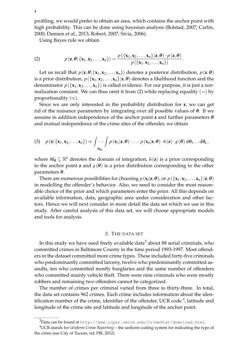
profiling, we would prefer to obtain an area, which contains the anchor point withhigh probability. This can be done using bayesian analysis (Bolstad, 2007; Carlin,2000; Damien et al., 2013; Robert, 2007; Sivia, 2006).

Using Bayes rule we obtain

(2) p(z,θ|{x1,x2, . . . ,xn}) =p({x1,x2, . . . ,xn}|z,θ) · p(z,θ)

p({x1,x2, . . . ,xn}).

Let us recall that p(z,θ|{x1,x2, . . . ,xn}) denotes a posterior distribution, p(z,θ)is a prior distribution, p({x1,x2, . . . ,xn}|z,θ) denotes a likelihood function and thedenominator p({x1,x2, . . . ,xn}) is called evidence. For our purpose, it is just a nor-malization constant. We can thus omit it from (2) while replacing equality (=) byproportionality (∝).

Since we are only interested in the probability distribution for z, we can getrid of the nuisance parameters by integrating over all possible values of θ. If weassume in addition independence of the anchor point z and further parameters θ

and mutual independence of the crime sites of the offender, we obtain

(3) p(z|{x1,x2, . . . ,xn})∝∫· · ·∫

Mθ

p(x1|z,θ) · . . . · p(xn|z,θ) ·h(z) ·g(θ) dθ1 . . .dθk ,

where Mθ ⊆ Rk denotes the domain of integration, h(z) is a prior correspondingto the anchor point z and g(θ) is a prior distribution corresponding to the otherparameters θ.

There are numerous possibilities for choosing p(xi|z,θ), or p({x1,x2, . . . ,xn}|z,θ)in modelling the offender’s behavior. Also, we need to consider the most reason-able choice of the prior and which parameters enter the prior. All this depends onavailable information, data, geographic area under consideration and other fac-tors. Hence we will next consider in more detail the data set which we use in thisstudy. After careful analysis of this data set, we will choose appropriate modelsand tools for analysis.

3. THE DATA SET

In this study we have used freely available data3 about 88 serial criminals, whocommitted crimes in Baltimore County in the time period 1993-1997. Most offend-ers in the dataset committed more crime types. These included forty-five criminalswho predominantly committed larceny, twelve who predominantly committed as-saults, ten who committed mostly burglaries and the same number of offenderswho committed mainly vehicle theft. There were nine criminals who were mostlyrobbers and remaining two offenders cannot be categorized.

The number of crimes per criminal varied from three to thirty-three. In total,the data set contains 962 crimes. Each crime includes information about the iden-tification number of the crime, identifier of the offender, UCR code 4, latitude andlongitude of the crime site and latitude and longitude of the anchor point.

3Data can be found at http://www.icpsr.umich.edu/CrimeStat/download.html.4UCR stands for Uniform Crime Reporting – the uniform coding system for indicating the type of

the crime (see City of Tucson, nd; FBI, 2012).

http://www.icpsr.umich.edu/CrimeStat/download.html


For the calculation of the distance and choice of the distance metric, we have todistinguish between geographic coordinate system and projected coordinate sys-tem. The use of the euclidean metric can lead to easier calculation – some func-tions can be expressed analytically. Additionally, all crime sites and anchor pointsof all offenders from the data set are located only in an area of 72,5km× 48,7km.Distances between a resident’s crime site and his anchor point are mostly a fewkilometers. Hence, the choice of a coordinate system, or the choice of a distancemetric should not lead to significantly different results.

Coordinates in the data set are recorded in the geographic coordinate system,thus, for using the euclidean metric we have to convert them into the plane co-ordinates. We use the most common projected coordinate system UTM (UniversalTransverse Mercator coordinate system) that divides the Earth between 84◦ S and 80◦

N latitude into 60 zones, each 6◦ of longitude in width (see Kennedy, 2000). To useEuclidean metric all investigated points have to lie in the same zone. Our data setis compliant for using this system because all points are located in the zone 18. Totransfer coordinates, we use a simplified version of relations which Johann HeinrichLouis Krüger derived in 1912 (see Kawase, 2011, 2012).

4. PROCEDURES AND MODELS

When analyzing the data set, we will generally assume as known the fact thatthe crime series was commited by the same offender. This assumption is realistic inpractice, since investigators may, according to the way the crime was commited,DNA analysis or other signs and evidence tell that the crimes are related to oneperson, just do not know which one and where to find him.

Different types of offenders require different models, hence we need to analyzecharacter of offenders in the given data set, and the way they choose the crime site.

4.1. Models for residents. First we will consider resident offenders5. They com-mit crimes near their anchor point. Hence their criminal and anchor regions over-lap, at least to a large extent. (see Fig. 1).

FIGURE 1. Anchor and criminal area of the resident offenders - the dashedline circle denotes the criminal area, the solid line circle is the anchor area,blue crosses indicate crime sites, the red circle is the anchor point of theoffender.

5Our division of offenders into two groups (residents and non-residents) is similar to the ma-rauder and the commuter hypothesis of Canter (1996). But in our case, the radius of the anchorarea is especially based on the distances of the crime sites from the anchor points of the observedoffenders. The criminal area can be imagined as the smallest circle that contains all crime sites ofthe given offender.

6

After analyzing the data set, we can classify offenders further into two subtypes,each of them requiring a different model.

E

N

4352

4354

4356

4358

4360

4362

4364

335 340 345 350 355

(A) Without a buffer zone.

E

N

4346

4348

4350

4352

4354

4356

4358

4360

350 355 360 365 370

(B) With a buffer zone.

FIGURE 2. Two basic subtypes of residents (red triangle indicates the crimesite, the black circle denotes the anchor point).

The two basic subtypes of residents (Fig. 2) are characterized by the existenceof a buffer zone. In both cases the distribution of crime sites is depicted on anapproximately same area 25km× 15km. However, in the first case the offendercommits crime in an immediate vicinity of the anchor point, having no buffer zone(see Fig. 2a). In the second case, the offender commits crimes several kilometresfrom the anchor point, hence there is some buffer zone (see Fig. 2b).

It was generally observed that if a resident has a small distance between crimesites (up to 2 km), the offender does not consider any buffer zone, and the be-havoiur is similar to the offender from Fig. 2a. Conversely, if the crime sites havelarger distances and the sites are irragularly spaced, the offender’s behaviour issimilar to that of Fig. 2b and we have to take some buffer zone into account

We can also observe residents whose crime sites create clusters (see Fig. 3),where the distances within some clusters are small, but larger within others.

E

N

4346

4347

4348

4349

4350

4351

4352

4353

4354

370 372 374

(A) Without a significant buffer zone.

E

N

4348

4350

4352

4354

4356

4358

4360

4362

362 364 366 368 370

(B) With a buffer zone.

FIGURE 3. Residents whose crime sites create clusters (The red triangleindicates the crime site, the black circle denotes the anchor point)).

Some residents with crime sites in clusters have similar bahavior as in Fig. 3a.They commit some crimes close to their anchor points, but other crimes in largerdistances. Distant crime sites can, but do not have to, create clusters. On the otherhand, some offenders (see Fig. 3b) create clusters although their anchor point doesnot occur in any of them. Such criminals only prefer some locations. Therefore,


if the crime sites of an offender create clusters or a cluster with other isolated anddistant crime sites, the offender can, but does not have to, create a buffer zonearound himself. In modelling we have to take this fact into account.

Undoubtedly, each criminal has an individuality with a unique behavior. Thus,we could find various specifics for all of them. However, the detailed examina-tion of our data set shows that each offender significantly tends to one of thesesubtypes. According to the space distribution of the criminal’s crime sites we candecide which subtype is the most suitable for the investigated offender. But in thecase of clusters we are not able to decide on the existence of the criminal’s bufferzone only on the basis of the space distribution of his crime sites.

For residents modelling we will use various modifications of the normal distri-bution. Compared to the use of the exponential distribution, the results are notsignificantly different. We use euclidean metrics for all models because it leads toan analytical expression for the models.

4.1.1. Residents without buffer zone and without clusters (subtype M1). For offenders,whose behaviour is similar to Fig. 2a, we will use a model suggested in O’Leary(2009a). Using Euclidean metric we obtain

(4) p(xi|z,α) =1

4α2 · exp(− π

4α2

[(x(1)i − z(1)

)2+(

x(2)i − z(2))2])

,

which corresponds to two dimensional normal distribution with mean at the an-

chor point and standard deviation σ =√

2π

α . The reason for this choice of σ canbe found in O’Leary (2009b). The parameter α denotes average distance that theoffender is willing to travel to commit a crime.

The most probable is committing crime directly at the anchor point or its imme-diate vicinity, which is exactly the behavior we expect for this type of offenders.Let us just remark that committing crime at the anchor point may seems strange,but is not at all impossible. In fact in our data set this situation occurs quite often,since the anchor point is not necessarily the offender’s place of residence, but hisfavourite bar, workplace, etc.

4.1.2. Residents with buffer zone and without clusters (subtype M2). For an offender asin Fig. 2b, the highest probability will not be at the anchor point, but some distanceα away from the anchor point, where α denote the average distance to the crimesite. This is captured by a probability distribution of the form

(5) p(xi|z,α,σ) =1

N (α,σ)· exp

− 12σ2

[√(x(1)i − z(1)

)2+(

x(2)i − z(2))2−α

]2 ,

where the choice of σ determines the decay of the probability as the distance variesfrom α .

In order to obtain a probability distribution, we must have(6)∫∫

R2

1N (α,σ)

· exp

− 12σ2

[√(x(1)i − z(1)

)2+(

x(2)i − z(2))2−α

]2 dx(1)i dx(2)i = 1 ,

A simple calculation gives the normalizing factor

(7) N (α,σ) = 2πσ2 · exp

(− α2

2σ2

)+2π

√2πασ

(1−Φ

(−α

σ

)),

8

where Φ is the distribution function of the standard normal distribution.

−4

−2

0

2

4

−4

−2

0

2

4

x(1)x(2)

(A) Three-dimensional plot.

x(1)

x(2

)

−4

−2

0

2

4

−4 −2 0 2 4

(B) Level plot.

FIGURE 4. Model for residents given by (5) with the anchor point z =

[0,0], α = 2 and σ = 0,8.

Fig. 4 illustrates a model for this type of residents. The anchor point is again theorigin, α = 2 a σ = 0,8. For different values of α a σ , the probability of committingcrime at the anchor point will be different, but nonzero, although for certain valuesvery close to zero. The buffer zone does not have to be interpreted as an area wherethe criminal commits no crimes, but as an area around the anchor point, with lowerprobability of commiting crimes. This interpretation corresponds better to reality,where we can hardly claim with certainty that there will be no crime in the bufferzone.

Remark. As defined, these offenders are called residents because their anchor and criminalareas overlap. However, they commit crimes at larger distances like non-residents (seeSubsection 4.2). If we choose an appropriate priors for angle and distance, we can use themodel of non-residents (see (10)) for this subtype of residents.

4.1.3. Residents with clusters (subtype M3). For offenders, whose crime sites createclusters, as in Fig. 3, we are not able to decide whether their anchor point liesaway from the clusters (they have a buffer zone), or whether it is in one of theclusters, and which one it is.

In this situation we will use multimodel inference (see Burnham et al., 2002;O’Leary, 2010b), where we obtain the resulting estimate as a weighted average ofthe estimates of anchor points in individual models, for the likelihood, or priordistribution. Let us assume that for estimating the anchor point we work withR models. We obtain as a result R posteriors, namely pi (z|{x1,x2, . . . ,xn}) for i =1,2, . . . ,R. The resulting estimate for multimodel inference is then

(8) p(z|{x1,x2, . . . ,xn}) =R

∑i=1

wi · pi (z|{x1,x2, . . . ,xn}) ,


where wi > 0 denotes the weight corresponding to the i-th estimate, and the weightssatisfy ∑

Ri=1 wi = 1. It guarantees that the resulting estimate also provides a prob-

ability distribution. For residents with R−1 clusters we will construct one modelfor each cluster and another model for the situation that the offender has a bufferzone.

The choice of weights depends on the analyst. If we have no reason to prefer oneof the models, we simply set wi =

1R for all i. We can also use previous results and

with offenders of a similar type find out which of the models better described thebehavior of the offender. According to the relativities we can then assign weightsto individual models. It is also possible that some evidence during the investiga-tion prefers one of the models. In this case we set the weights based on preferencesof an experienced investigator.

4.2. Models for non-residents. Non-resident is an offender who commits crimesrelatively far from his anchor point (see Fig. 5).

FIGURE 5. Anchor and criminal area of the non-resident offenders - thedashed line circle denotes the criminal area, the solid line circle is the anchorarea, blue crosses indicate crime sites, the red circle is the anchor point ofthe offender.

The criminal and anchor areas essentially do not overlap in this case. However,it does not mean that this area is unknown for the criminal. It is only significantlyaway from the territory in which he normally lives, works and acts as a "non-offender".

In our dataset, non-residents typically commit crimes at a distance greater than10 km, but it is often at least twice that distance. Another specific feature for thistype of offenders is that they prefer a certain angle (measured from the horizontalaxis with the origin at the anchor point) for the choice of their crime location.

In our dataset, there is just a small number of non-residents and we did notobserve any markedly different behavior among them. Therefore we do not dividethis type of offenders into other subtypes as in the case of residents in the previoussubsection.

In Mohler and Short (2012), there is used a kinetic model that is derived on thebasis of the following stochastic differential equation

(9) dxt = µ(xt)+√

2DdWt ,

where x(t) denotes the position of the offender at time t, Wt is two-dimensionalstandard Wiener process, D denotes the diffusion parameter and µ is the drift.The drift term could be used to describe more complex criminal behavior.

10

For different choices of the parameter values, the model is suitable for differenttype of offenders. If we want to obtain the most realistic model which is applicableto non-residents, we have to use numerical methods. However, the solution can beapproximated by the product of a function of the distance and a function of the an-gle (again measured from the horizontal axis with the origin at the anchor point).This fact supports the idea that the criminal behavior could be generally mod-eled as the product of a suitable function which influences the most likely distancefrom the offender’s anchor point and another function that affects probability ofthe angle preferred by the criminal.

Again, the model is based on the normal distribution, and is given by

(10) p(xi|z,α,ϑ ,σ1,σ2) =1

N (α,ϑ ,σ1,σ2)·q1 (xi|z,α,σ1) ·q2 (xi|z,ϑ ,σ2) ,

where

(11) q1 (xi|z,α,σ1) = exp

− 12σ2

1

[√(x(1)i − z(1)

)2+(

x(2)i − z(2))2−α

]2

and

(12) q2 (xi|z,ϑ ,σ2) = exp(− 1

2σ22

[arg((

x(1)i − z(1))+ i(

x(2)i − z(2)))−ϑ

]2),

where α is the average distance of the offenses, σ1 denotes the standard deviationcorresponding to the function q1, ϑ is the average angle from the anchor point tothe crime locations measured from the horizontal axis with the origin at the anchorpoint, and σ2 denotes the standard deviation corresponding to the function q2 (seeFig. 6).

The use of the function q1 is analogous to the model (5) for residents with bufferzone, and therefore it can be interpreted in the same way. The function q2 achievesthe highest values at the angle of ϑ and its functional values around this angledecrease at a rate that depends on the choice of the value of σ2. This functionitself cannot be normalized since the double integral over all its possible values isinfinite. But the product of q1 and q2 in (10) can already be normalized.

Let us note that the normalization factor has the form

(13) N (α,ϑ ,σ1,σ2) = N1 (α,σ1) ·N2 (ϑ ,σ2) ,

where

(14) N1 (α,σ1) = σ21 · exp

(− α2

2σ21

)+√

2πασ1

(1−Φ

(− α

σ1

))and

(15) N2 (ϑ ,σ2) = σ2√

2π

(Φ

(2π−ϑ

σ2

)−Φ

(− ϑ

σ2

)),

where Φ represents the distribution function of the standard normal distribution.We obtain this value of the normalization factor from the requirement that thefunction p in (10) has to be a probability density, hence

(16)∫∫R2

1N (α,ϑ ,σ1,σ2)

·q1 (xi|z,α,σ1) ·q2 (xi|z,ϑ ,σ2) dx(1)i dx(2)i = 1 .

If we know in advance whether the offender is a resident or a non-resident, wechoose an appropriate function as proposed above, to model his behavior. For


−4−2

02

4

−4

−2

0

2

4

x(1)

x(2)


x(1)

x(2)

−4

−2

0

2

4

−4 −2 0 2 4

(B) Level plot.

FIGURE 6. The function given by (10) with the anchor point z = [0,0],α = 2, σ1 =

45 ,ϑ = π

4 and σ2 =π

6 .

residents, we have to decide on the offender’s subtype based on the distributionof the criminal’s crime locations.

If we are not able to determine in advance, whether the offender is a resident ora non-resident, we can use multimodel inference again, as discussed in Subsection4.1.

5. THE CHOICE OF A PRIOR DISTRIBUTION

When processing the dataset, we work with offenders of different types andsubtypes. Depending on a specific offender, we need to select appropriate priorsfor the parameters. In this study, we used kernel smoothing, and logspline densityestimation (see for example Kooperberg and Stone, 1991), which allows to limit therange of values that the parameter can take. We always assume that all informa-tion about each offender contained in the data set is known to us. We only excludeknowledge about the examined offender 6.

Picture 7 graphically represents our prior for the anchor point. To obtain it, weused kernel smoothing, based on the anchor points of known offenders.

Next, we need to know the prior for average distance α to the offence. Sincethe distance cannot take negative values we use logspline density estimation withlower limit equal to zero. In this case, however, we have to use solely the datacorresponding to the particular types of offenders. This is because the distance isjust one of the main factors that the types and subtypes of offenders differ fromone another. The function g1 (α) corresponds to the subtype M1, the g2 (α) to thesubtype M2 and the function g3 (α) is obtained from the known average distancefor non-residents and it will be used for this type of offenders. These functions areillustrated in Fig. 8.

If we use the model given by (10), we have to know the prior distribution forthe angle ϑ . In Figure 9 we plot the estimated distribution of ϑ for offenders ofsubtype M2 and for non-residents. We can see that offenders of subtype M2 prefer

6Although all information in the dataset is known to us, in the following paragraphs we willuse the word “known” for the data of all offenders except the investigated criminal.

12

300320

340360

380400

4340

4360

4380

4400

x(1)x(2)


x(1)

x(2)

4340

4360

4380

320 340 360 380

(B) Level plot.

FIGURE 7. Graphical representation of the prior h(z) for the anchor point.

α0 10 20 30 40

α0 10 20 30 40

α0 10 20 30 40

g1(α

)

g2(α

)

g3(α

)

FIGURE 8. Graphical representation of the prior g1 (α) (solid line), g2 (α)

(dashed line) and g3 (α) (dash-dotted line) for the average distance α , thatthe offender is willing to travel to commit a crime.

angle between π

2 and π , non-residents favour more directions -– the south-westdirection (angle between π and 3

2π) and east direction (angle around 0, or 2π).Significant preference of some directions can be caused by the existence of majortransport networks for these angles.

ϑ (radians) − subtype M2

0.0

0.1

0.2

0.3

0.4

0.5

0 2 4 6

ϑ (radians) − commuters

0.0

0.2

0.4

0.6

0 2 4 6

FIGURE 9. Histograms of the average angle ϑ (measured from the horizon-tal axis with the origin at the anchor point), in which the offender commitscrimes - for residents M2 and for non-residents.


Similarly we obtain prior distribution for other required parameters.

6. MODELLING AND EVALUATION

In Section 4 we considered four types of offenders (residents M1, M2 and M3and non-residents). For modelling of each of these types we can choose some ofthree models given by (4), (5) and (10), or use multimodel inference, a combinationof some of them.

Based on this, we will separate the modelling with our dataset into the followingcases:

(1) We choose only residents from the dataset.(a) For modelling of residents M1 we use the model (4), for residents M2

the model given by (5), for residents M3 we use multimodel inference,a combination of (4) and (5).

(b) For modelling of residents M1 we use the model (4), for residents M2the model given by (10), for residents M3 we use multimodel inference,a combination of (4) and (10).

(2) We deal with all offenders without knowing in advance the type of the in-vestigated offender. For each offender we admit the possibility that theoffender is a resident of a certain type or a non-resident. Then we appro-priately combine these two possibilities.(a) For modelling of residents M1 we use the model (4), for residents M2

the model given by (5), for residents M3 we use multimodel inference,a combination of (4) and (5), for non-residents the model (10).

(i) Multimodelling weights are the same both for residents and fornon-residents.

(ii) Multimodelling weights for residents and non-residents are de-rived by frequencies of these types in our dataset.

(b) For modelling of residents M1 we use the model (4), for residents M2the model given by (10), for residents M3 we use multimodel inference,a combination of (4) and (10), for non-residents the model (10).

(i) Multimodelling weights are the same both for residents and fornon-residents.

(ii) Multimodelling weights for residents and non-residents are de-rived by frequencies of these types in our dataset.

We compare these methods with Rossmo’s approach. Rossmo works with hitscore function given by (1) and distance decay function of the form

(17) f (d (xi,y)) =

k

(d (xi,y))h pro d (xi,z)> b

kbg−h

(2b−d (xi,y))g pro d (xi,z)6 b ,

where b denotes the radius of the buffer zone, distance d (xi,z) is calculated by theManhattan metric and exponents f and g are equal to 1,2. These values of the pa-rameters are recommended by Rossmo based on his research. We set the value ofthe parameter b equal one half of the average distance of the nearest neighbourbetween crimes in the given crime series 7. The choice of parameter k is not im-portant because the hit score function is the sum of the individual distance decayfunctions, the values of the hit score function are compared among themselves.

7This choice for the parameter b is presented eg. in Raine et al. (2009).

14

The constant multiplies these values of the hit score function but does not changeratios between them. Rossmo’s formula assumes that the offender’s anchor pointis located close to his crime sites (how close – it depends on the optional parameterb). This is the reason why this relationship is suitable especially for residents.

Let the investigated jurisdiction lie in the area of the rectangle with sides 100 kmand 70 km, defined by the UTM coordinates 300 km west, 400 km east, 4330 kmsouth and 4400 km north 8. We divide this rectangle into a grid 70 × 100, thus thedimensions of each cell are approximately 1,4 km × 1,4 km.

For each investigated offender we plot his crime locations. Based on the spacedistribution, distances between crimes and occurrence or absence of clusters, wecan determine the most appropriate criminal type, or subtype for the given of-fender. According to this type we choose a suitable model.

If we only deal with residents, in each cell of jurisdiction we evaluate the poste-rior for the considered methods described at the beginning of this section and forRossmo’s approach. In the case when we examine all criminals without knowingthe type (resident or non-resident) of the offender, we evaluate also the posteriorin each cell for the situation that the criminal is a non-resident. Then we multiplythe posterior for residents and the posterior for non-residents by the appropriateweights and after their sum we obtain an estimate of the anchor point z, if the of-fender committed crimes in locations x1,x2, . . . ,xn. Again, we apply this processto all methods described at the beginning of this section and compare them withRossmo’s approach.

For each method we order all cells based upon the value of the posterior, fromhighest to lowest, thus from the cell that contains the anchor point with the highestprobability to the cell that includes the anchor point with the lowest probability.The efficiency of the method depends on how many cells we have to examine untilwe find the anchor point of the investigated offender. If we divide this number ofcells by the total number of cells in the given jurisdiction, we obtain the percentageof the area that we have to explore to find the offender’s anchor point. Thus, themethod with the lowest percentage is the most effective for the particular series.

Figure 10 shows a comparison of methods [1a], [1b] and Rossmo’s approachin terms of this evaluation. We only selected residents from the dataset; we didnot consider the possibility that any of the criminals could be a non-resident. Al-though Rossmo’s approach is appropriate just for residents, both methods [1a]and [1b] indicate better, and very similar, efficiency.

Fig. 11 gives a comparison of methods [2ai] and [2bi] and Rossmo’s approach(Fig. 11a and Fig. 11c) in terms of the described means of evaluation. It also com-pares methods [2aii] and [2bii] and Rossmo’s approach (Fig. 11b and Fig. 11d).Now we consider all offenders without knowing the type of each criminal. Wecan see that Rossmo’s approach almost always exhibits the lowest efficiency inboth cases. However, the difference between efficiencies of the methods is not asremarkable as in the situation considered above when we dealt only with resi-dents. Due to the inclusion of all criminals to the analysis, the estimation of theanchor point for methods [2ai], [2bi] and [2aii], [2bii] worsened for residents sincewe had to admit the possibility that the investigated offender is a non-resident.These methods achieve better results for non-residents than Rossmo’s approach.

8The size of the jurisdiction was chosen to include all crimes and anchor points in the dataset ±approximately 5 km.


Fraction of explored cells

Fra

ctio

n of

foun

d an

chor

poi

nts

0.00 0.05 0.10 0.15

0.0

0.2

0.4

0.6

0.8

1.0

●

●

●● ● ● ● ● ● ● ● ● ● ● ● ● ● ●

(A) Normal scale.


Fra

ctio

n of

foun

d an

chor

poi

nts

0.00 0.05 0.10 0.15

0.80

0.85

0.90

0.95

1.00

●

●

● ●

● ● ●

● ● ● ● ● ● ● ● ● ●

(B) Detail.

FIGURE 10. The relationship between the proportion of the found anchorpoints and the proportion of the explored area, when we only deal withresidents; method [1a] (red circles), method [1b] (blue squares), Rossmo’sapproach (green triangles).

However, in our datasets, non-residents constitute only 111 of all offenders (it cor-

responds to the choice of multimodel weights for methods [2aii] and [2bii]).Nevertheless, we can say, that methods [2ai], [2bi] and [2aii], [2bii] exhibit bet-

ter results than Rossmo’s approach (although due to the previous case when wedealt only with residents the difference between the results of the considered ap-proaches is not so significant). We can assume even higher efficiency for datasetswith greater proportion of non-residents. We can see that for our dataset, the bestchoice for residents with buffer zone in both cases is the model of the form (10).The option of multimodel weights distinguishes considered method as expected.If we assign the same weights to both types of criminals (Fig. 11a, respectivelyFig. 11c), non-residents are caught earlier. On the contrary, the choice of weightsbased on frequencies of the types in the dataset (Fig. 11b, respectively Fig. 11d),when the weight for the model of residents corresponds to the value of w1 = 10

11and for the model of non-residents takes the value of w2 =

111 , , leads to earlier cap-

turing of residents at the expense of later finding of non-residents. Overall, Fig.11 shows that the use of the prior knowledge about the structure of the dataset todetermining the weights results in faster capture of a larger part of the offenders.

In Fig. 12 we can see estimates of the offender’s anchor point – for each case weuse the method [2ai] and Rossmo’s approach. For residents without buffer zone,both methods are similarly effective (Fig. 12a and 12b). However, in the case ofresidents with buffer zone (Fig. 12c and 12d) and also in the case of non-residents(Fig. 12e and 12f), the hit score function using Rossmo’s distance decay functionstill assumes that the anchor point lies close to any of the offender’s crime sites.Conversely, the model [2ai] admits the possibility that the criminal’s anchor pointis located at a greater distance from his crime sites.

7. CONCLUSION

We offered a more complex approach, how to treat the problem of geographicprofiling. After analyzing the data set on serial criminals from certain area, we canobserve similar tendencies for choosing the crime site. Based on this, we classifythe criminals into different types. It often turns out that similar distribution of

16


Fra

ctio

n of

foun

d an

chor

poi

nts

0.00 0.05 0.10 0.15

0.0

0.2

0.4

0.6

0.8

1.0

●

●

●

●● ●

● ● ●●

● ● ● ● ● ● ● ●

(A) The same weights for model of residents andmodel of non-residents.


Fra

ctio

n of

foun

d an

chor

poi

nts

0.00 0.05 0.10 0.15

0.0

0.2

0.4

0.6

0.8

1.0

●

●

●●

● ●● ●

●● ● ● ● ● ● ● ● ●

(B) The weights according to the frequencies ofresidents and non-residents in our data set.


Fra

ctio

n of

foun

d an

chor

poi

nts

0.00 0.05 0.10 0.15

0.80

0.85

0.90

0.95

1.00

●

●

● ●

●

● ●

●

● ● ● ● ● ● ● ●

(C) The same weights for model of residents andmodel of non-residents (detail).


Fra

ctio

n of

foun

d an

chor

poi

nts

0.00 0.05 0.10 0.15

0.80

0.85

0.90

0.95

1.00

●

●

●

● ●

● ●

●

● ● ● ●

● ● ● ● ●

(D) The weights according to the frequencies ofresidents and non-residents in our data set (de-tail).

FIGURE 11. The relationship between the proportion of the found anchorpoints and the proportion of the explored area, when we deal with all offend-ers without knowing their types in advance. The parts (a) and (c): method[2ai] (red circles), method [2bi] (blue squares), Rossmo’s approach (greentriangles); The parts (b) and (d): method [2aii] (red circles), method [2bii](blue squares), Rossmo’s approach (green triangles).

crime sites corresponds to very similar behaviour when choosing the crime site.Thanks to this we can, for a given criminal, construct a model based on behaviourof criminals of the same type.

We divided offenders from our data set into two basic groups – residents andnon-residents. This distinction is very similar to the marauder and the commuterhypothesis. Main idea of the overlap of criminal and anchor area is the same. Butmodels, which are able to describe the behaviour of commuters (in our case non-residents) are very rare in the literature. One of the few is suggested in the paper ofMohler and Short (see Mohler and Short, 2012). Their approach, based on solvinga stochastic differential equation, leads to a model which for a suitable choice ofparameters characterizes well the nature of commuters (non-residents). Here weoffered a simpler, purely bayesian model, which preserves the main features andflexibility of models suggested in Mohler and Short (2012).


x(1)

x(2

)

4340

4360

4380

320 340 360 380

●

(A) Model [2ai] for a resident without a bufferzone.

x(1)

x(2

)

4340

4360

4380

320 340 360 380

●

(B) Rossmo’s model for a resident without abuffer zone.

x(1)

x(2

)

4340

4360

4380

320 340 360 380

●

(C) Model [2ai] for a resident with a buffer zone.

x(1)

x(2

)

4340

4360

4380

320 340 360 380

●

(D) Rossmo’s model for a resident with a bufferzone.

x(1)

x(2

)

4340

4360

4380

320 340 360 380

●

(E) Model [2ai] for a non-resident.

x(1)

x(2

)

4340

4360

4380

320 340 360 380

●

(F) Rossmo’s model for a non-resident.

FIGURE 12. Level plots indicating how likely is that the area contains theanchor point of the offender (regions with the highest probability are pink,areas with the lowest probability are blue). The red triangles denote crimesites of the offender, the black circle indicates his anchor point.

Considered models better capture the criminal’s behaviour than the models ofO’Leary (2009a), since our setup is based on data from similarly behaving crimi-nals. At the same time, they are easier to apply and interpret than the models ofMohler and Short, while keeping the ability to cover a broad spectrum of offenders.Second, the paper showed how to distinguish the types of offenders based on thespatial distribution of their crime sites.

In case we were not able to asign the given criminal to a certain group of alreadyinvestigated criminals, it was natural to use multimodel inference. It allows to

18

incorporate into the model all possibilities which we consider. In particular, thisapproach was used to deal with the case when the criminal can be a resident ora non-resident. In our case it turned out that it is suitable to derive weights formultimodel inference by frequencies of residents and non-residents in the dataset.

We used the standard Rossmo’s model as a benchmark. Our model substantiallyoverperformed the benchmark, especially in the presence of non-residents.


REFERENCES

Bolstad, W. M. (c2007). Introduction to Bayesian statistics. John Wiley, Hoboken, N.J.,2nd ed. edition.

Brantingham, P. L. and Brantingham, P. J. (1993). Nodes, paths and edges. Journalof Environmental Psychology, 13(1):3–28.

Burnham, K. P., Anderson, D. R., and Burnham, K. P. (c2002). Model selection andmultimodel inference. Springer, New York, 2nd ed. edition.

Canter, D. (1996). Psychology in action. Dartmouth, Aldershot, England Brookfield,Vt., USA.

Canter, D., Coffey, T., Huntley, M., and Missen, C. (2000). Predicting serial killers’home base using a decision support system. Journal of Quantitative Criminology,16(4):457–478.

Carlin, B. (2000). Bayes and Empirical Bayes methods for data analysis. Chapman &Hall/CRC, Boca Raton.

City of Tucson (n.d.). Uniform crime reporting codes. Retrieved March 8, 2014,from http://www.tucsonaz.gov/police/ucr-codes.

Damien, P., Dellaportas, P., Polson, N. G., Stephens, D. A., and Smith, A. F. (2013).Bayesian theory and applications. Oxford University Press, Oxford, first edition.edition.

FBI (2012). Uniform crime reports. Retrieved March 8, 2014, from http://www.fbi.gov/about-us/cjis/ucr.

Kawase, K. (2011). A general formula for calculating meridian arc length and itsapplication to coordinate conversion in the gauss-krüger projection. Bulletin ofthe Geospatial Information Authority of Japan, 59:1–13.

Kawase, K. (2012). The environmental range of serial rapists. Bulletin of the Geospa-tial Information Authority of Japan, 60:1–6.

Kennedy, M. (2000). Understanding map projections : GIS by ESRI. ESRI, Redlands,CA.

Kooperberg, C. and Stone, C. J. (1991). A study of logspline density estimation.Computational Statistics & Data Analysis, 12(3):327–347.

Levine, N. (2008). Crimestat: A spatial statistical program for the analysis of crimeincidents. In Encyclopedia of GIS, pages 187–193. Springer US.

Mohler, G. O. and Short, M. B. (2012). Geographic profiling from kinetic modelsof criminal behavior. SIAM Journal on Applied Mathematics, 72(1):163–180.

O’Leary, M. (2009a). The mathematics of geographic profiling. Journal of Investiga-tive Psychology and Offender Profiling, 6(3):253–265.

O’Leary, M. (2009b). A new mathematical approach to geographic profiling. Tow-son University.

O’Leary, M. (2010a). Implementing a bayesian approach to criminal geographicprofiling. In Proceedings of the 1st International Conference and Exhibition on Com-puting for Geospatial Research & Application, pages 59:1–59:8, New York, NY, USA.ACM.

O’Leary, M. (2010b). Multimodel inference and geographic profiling. Crime Map-ping, 2(1).

Raine, N. E., Rossmo, D. K., and Le Comber, S. C. (2009). Geographic profilingapplied to testing models of bumble-bee foraging. Journal of The Royal SocietyInterface, 6(32):307–319.

Robert, C. (2007). The Bayesian choice from decision-theoretic foundations to computa-tional implementation. Springer, New York.

http://www.tucsonaz.gov/police/ucr-codes

http://www.fbi.gov/about-us/cjis/ucr

http://www.fbi.gov/about-us/cjis/ucr

20

Rossmo, D. (2000). Geographic profiling. CRC Press, Boca Raton, Fla.Rossmo, D. K. (1995). Geographic profiling: Target patterns of serial murderers. PhD

thesis, Theses (School of Criminology)/Simon Fraser University.Sivia, D. S. (2006). Data analysis a Bayesian tutorial. Oxford University Press, Oxford

New York.

GEOGRAPHIC PROFILING: BAYESIAN MODELS FOR …kolacek/docs/English1.pdf · GEOGRAPHIC PROFILING:...

Documents

Transcript of GEOGRAPHIC PROFILING: BAYESIAN MODELS FOR …kolacek/docs/English1.pdf · GEOGRAPHIC PROFILING:...