1

Generating Electricity through

Induction Using a Magnetic Field to

Power a Pendulum

Thorsen M. Wehr Odessa Junior High School, Odessa, WA 99159

Abstract Harsh pollutants of energy producing methods such as coal and gasoline have people looking for a

solution. When Michael Faraday made his discovery of electromagnetic induction in 1831, he

hypothesized a changing magnetic field was necessary to induce a current in a nearby circuit.

Regarding this project, an energy source based on magnetic fields might give zero pollutants.

After some research, it was concluded that a magnet attached to the end of a swinging pendulum

passing over a coil of wound copper might produce electricity. After three attempts, a final design

was made allowing the magnet at the base of the pendulum arm to attract metal plates at each side

of the pendulum's period. Based on statistical data, the magnet and metal plates made a positive

difference to the swing time compared to the control method. The 45cm experimental method had

an average swing time of 132.6 seconds and the control trials had an average swing time of 111.3

seconds. An average of 50.9 volts was created by the control method and 59.5 volts was created

by the experimental method. If the coils lengths were 10 meters, they would make 542kWh/year

added to 600kWh/year by lengthening the pendulum arm, and a total of 1,142Wh/year could be

generated. Future plans will be to make the controlled swing time longer, which will increase the

experimental time, and increase the amount of electricity produced. Hopefully, a larger scale of

this device could be the answer to a cleaner and renewable energy source.

Introduction

Magnets are used to make life easier. Many examples of this are already in use such as

Maglev trains. This is done by magnets, making it possible for the vehicle to float above

its track. Furthermore, Maglev trains are energy-efficient and extremely reliable and safe.

Another such example might be simple refrigerator magnets used to hold notes or papers.

Currently, the most powerful magnets are Neodymium magnets, a rare earth metal with atomic

number of 60 and symbol of Nd. These magnets are significantly stronger than any other magnet

on Earth; equivalent magnet lifting strength is about 3 to 5 times as much for the equivalent mass

(Physics Van Outreach Program, 2010). All of these examples are of using the magnet to do a

task, but is it possible to use the energy from the magnet to produce clean electrical energy?

2

Coal and gasoline are such methods for producing energy like how gasoline moves your car.

As great of a solution to our transportation problem as this is, gasoline is a fossil fuel, and will

eventually run out, and also emit harmful gases such as CO2. In 2006, the average CO2 output

was over 1.2 million tons in America and parts of Europe (Collins, 2006) (Figure 1). That is a

lot of pollution that damages the environment and ozone, which is important for the survival of

life.

When Michael Faraday made his discovery of electromagnetic induction in 1831, he

hypothesized that a changing magnetic field is necessary to induce a current in a nearby circuit.

To test his hypothesis he made a coil by wrapping a paper cylinder with copper wire. He

connected the coil to a galvanometer, and then moved a magnet back and forth inside the

cylinder (Figure 2). Since the copper wires contain a changing electric charge, an object placed

within the electric field will become charged. When the magnet is pushed in and out of the coils,

the magnetic field around the coils is changed. This in turn makes the electrons in the coil move,

Figure 1. The average amount of CO2 emissions per year.

The key shows color coding for the countries and all the

CO2 per country (Collins, 2006).

3

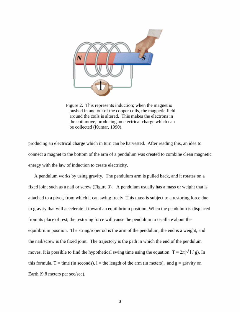
Figure 2. This represents induction; when the magnet is

pushed in and out of the copper coils, the magnetic field

around the coils is altered. This makes the electrons in

the coil move, producing an electrical charge which can

be collected (Kumar, 1990).

producing an electrical charge which in turn can be harvested. After reading this, an idea to

connect a magnet to the bottom of the arm of a pendulum was created to combine clean magnetic

energy with the law of induction to create electricity.

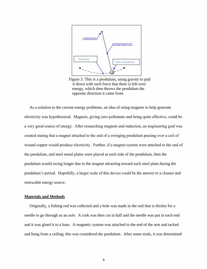
A pendulum works by using gravity. The pendulum arm is pulled back, and it rotates on a

fixed joint such as a nail or screw (Figure 3). A pendulum usually has a mass or weight that is

attached to a pivot, from which it can swing freely. This mass is subject to a restoring force due

to gravity that will accelerate it toward an equilibrium position. When the pendulum is displaced

from its place of rest, the restoring force will cause the pendulum to oscillate about the

equilibrium position. The string/rope/rod is the arm of the pendulum, the end is a weight, and

the nail/screw is the fixed joint. The trajectory is the path in which the end of the pendulum

moves. It is possible to find the hypothetical swing time using the equation: T = 2π(√ l / g). In

this formula, T = time (in seconds), l = the length of the arm (in meters), and g = gravity on

Earth (9.8 meters per sec/sec).

4

Figure 3. This is a pendulum, using gravity to pull

it down with such force that there is left-over

energy, which then throws the pendulum the

opposite direction it came from.

As a solution to the current energy problems, an idea of using magnets to help generate

electricity was hypothesized. Magnets, giving zero pollutants and being quite effective, could be

a very good source of energy. After researching magnets and induction, an engineering goal was

created stating that a magnet attached to the end of a swinging pendulum passing over a coil of

wound copper would produce electricity. Further, if a magnet system were attached to the end of

the pendulum, and steel metal plates were placed at each side of the pendulum, then the

pendulum would swing longer due to the magnet attracting toward each steel plate during the

pendulum’s period. Hopefully, a larger scale of this device could be the answer to a cleaner and

renewable energy source.

Materials and Methods

Originally, a fishing rod was collected and a hole was made in the end that is thicker for a

needle to go through as an axle. A cork was then cut in half and the needle was put in each end

and it was glued it to a base. A magnetic system was attached to the end of the arm and tacked

and hung from a ceiling; this was considered the pendulum. After some trials, it was determined

Trajectory End of pendulum

5

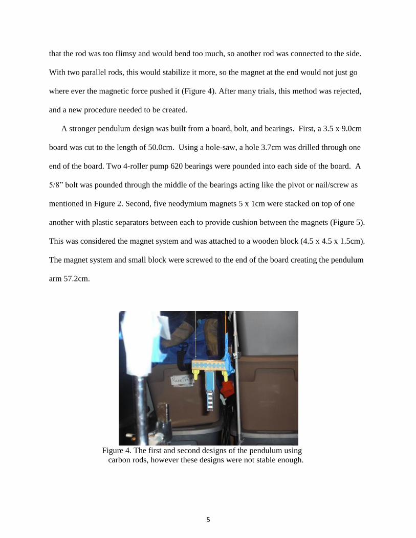
that the rod was too flimsy and would bend too much, so another rod was connected to the side.

With two parallel rods, this would stabilize it more, so the magnet at the end would not just go

where ever the magnetic force pushed it (Figure 4). After many trials, this method was rejected,

and a new procedure needed to be created.

A stronger pendulum design was built from a board, bolt, and bearings. First, a 3.5 x 9.0cm

board was cut to the length of 50.0cm. Using a hole-saw, a hole 3.7cm was drilled through one

end of the board. Two 4-roller pump 620 bearings were pounded into each side of the board. A

5/8” bolt was pounded through the middle of the bearings acting like the pivot or nail/screw as

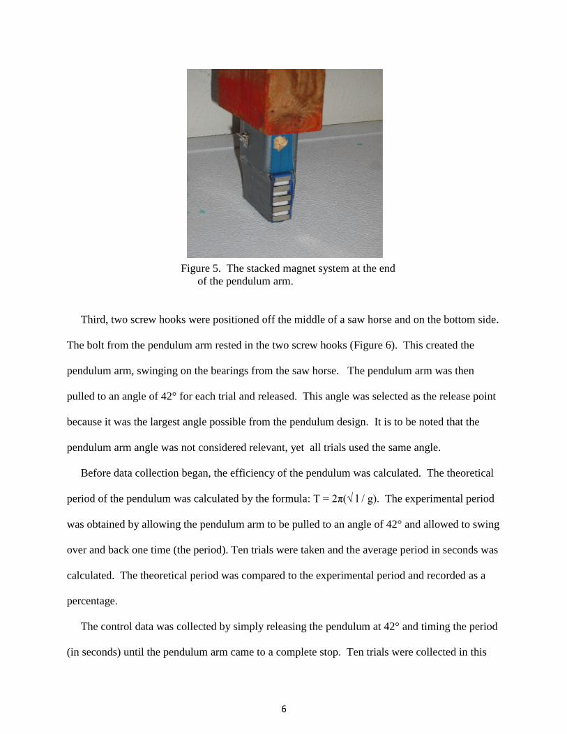
mentioned in Figure 2. Second, five neodymium magnets 5 x 1cm were stacked on top of one

another with plastic separators between each to provide cushion between the magnets (Figure 5).

This was considered the magnet system and was attached to a wooden block (4.5 x 4.5 x 1.5cm).

The magnet system and small block were screwed to the end of the board creating the pendulum

arm 57.2cm.

Figure 4. The first and second designs of the pendulum using

carbon rods, however these designs were not stable enough.

6

Figure 5. The stacked magnet system at the end

of the pendulum arm.

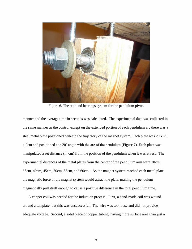
Third, two screw hooks were positioned off the middle of a saw horse and on the bottom side.

The bolt from the pendulum arm rested in the two screw hooks (Figure 6). This created the

pendulum arm, swinging on the bearings from the saw horse. The pendulum arm was then

pulled to an angle of 42° for each trial and released. This angle was selected as the release point

because it was the largest angle possible from the pendulum design. It is to be noted that the

pendulum arm angle was not considered relevant, yet all trials used the same angle.

Before data collection began, the efficiency of the pendulum was calculated. The theoretical

period of the pendulum was calculated by the formula: T = 2π(√ l / g). The experimental period

was obtained by allowing the pendulum arm to be pulled to an angle of 42° and allowed to swing

over and back one time (the period). Ten trials were taken and the average period in seconds was

calculated. The theoretical period was compared to the experimental period and recorded as a

percentage.

The control data was collected by simply releasing the pendulum at 42° and timing the period

(in seconds) until the pendulum arm came to a complete stop. Ten trials were collected in this

7

Figure 6. The bolt and bearings system for the pendulum pivot.

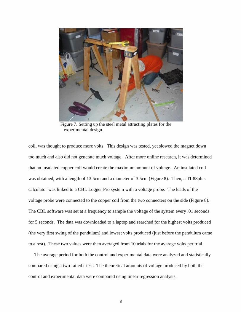
manner and the average time in seconds was calculated. The experimental data was collected in

the same manner as the control except on the extended portion of each pendulum arc there was a

steel metal plate positioned beneath the trajectory of the magnet system. Each plate was 20 x 25

x 2cm and positioned at a 20˚ angle with the arc of the pendulum (Figure 7). Each plate was

manipulated a set distance (in cm) from the position of the pendulum when it was at rest. The

experimental distances of the metal plates from the center of the pendulum arm were 30cm,

35cm, 40cm, 45cm, 50cm, 55cm, and 60cm. As the magnet system reached each metal plate,

the magnetic force of the magnet system would attract the plate, making the pendulum

magnetically pull itself enough to cause a positive difference in the total pendulum time.

A copper coil was needed for the induction process. First, a hand-made coil was wound

around a template, but this was unsuccessful. The wire was too loose and did not provide

adequate voltage. Second, a solid piece of copper tubing, having more surface area than just a

8

Figure 7. Setting up the steel metal attracting plates for the

experimental design.

coil, was thought to produce more volts. This design was tested, yet slowed the magnet down

too much and also did not generate much voltage. After more online research, it was determined

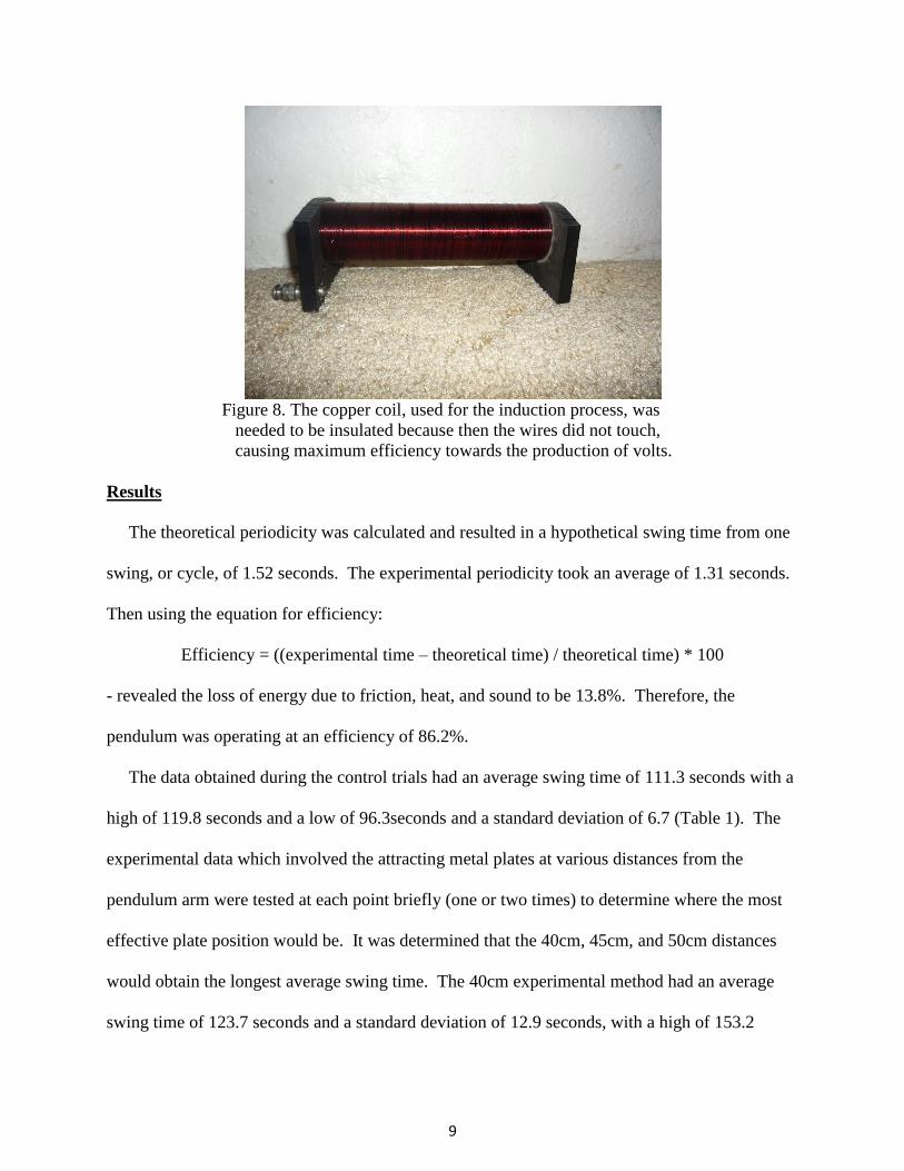
that an insulated copper coil would create the maximum amount of voltage. An insulated coil

was obtained, with a length of 13.5cm and a diameter of 3.5cm (Figure 8). Then, a TI-83plus

calculator was linked to a CBL Logger Pro system with a voltage probe. The leads of the

voltage probe were connected to the copper coil from the two connecters on the side (Figure 8).

The CBL software was set at a frequency to sample the voltage of the system every .01 seconds

for 5 seconds. The data was downloaded to a laptop and searched for the highest volts produced

(the very first swing of the pendulum) and lowest volts produced (just before the pendulum came

to a rest). These two values were then averaged from 10 trials for the avarege volts per trial.

The average period for both the control and experimental data were analyzed and statistically

compared using a two-tailed t-test. The theoretical amounts of voltage produced by both the

control and experimental data were compared using linear regression analysis.

9

Figure 8. The copper coil, used for the induction process, was

needed to be insulated because then the wires did not touch,

causing maximum efficiency towards the production of volts.

Results

The theoretical periodicity was calculated and resulted in a hypothetical swing time from one

swing, or cycle, of 1.52 seconds. The experimental periodicity took an average of 1.31 seconds.

Then using the equation for efficiency:

Efficiency = ((experimental time – theoretical time) / theoretical time) * 100

- revealed the loss of energy due to friction, heat, and sound to be 13.8%. Therefore, the

pendulum was operating at an efficiency of 86.2%.

The data obtained during the control trials had an average swing time of 111.3 seconds with a

high of 119.8 seconds and a low of 96.3seconds and a standard deviation of 6.7 (Table 1). The

experimental data which involved the attracting metal plates at various distances from the

pendulum arm were tested at each point briefly (one or two times) to determine where the most

effective plate position would be. It was determined that the 40cm, 45cm, and 50cm distances

would obtain the longest average swing time. The 40cm experimental method had an average

swing time of 123.7 seconds and a standard deviation of 12.9 seconds, with a high of 153.2

10

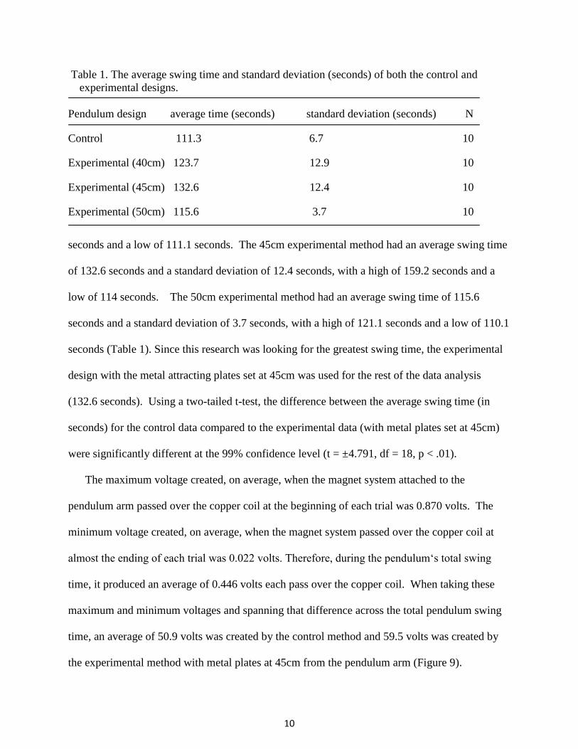
Table 1. The average swing time and standard deviation (seconds) of both the control and

experimental designs.

Pendulum design average time (seconds) standard deviation (seconds) N

Control 111.3 6.7 10

Experimental (40cm) 123.7 12.9 10

Experimental (45cm) 132.6 12.4 10

Experimental (50cm) 115.6 3.7 10

seconds and a low of 111.1 seconds. The 45cm experimental method had an average swing time

of 132.6 seconds and a standard deviation of 12.4 seconds, with a high of 159.2 seconds and a

low of 114 seconds. The 50cm experimental method had an average swing time of 115.6

seconds and a standard deviation of 3.7 seconds, with a high of 121.1 seconds and a low of 110.1

seconds (Table 1). Since this research was looking for the greatest swing time, the experimental

design with the metal attracting plates set at 45cm was used for the rest of the data analysis

(132.6 seconds). Using a two-tailed t-test, the difference between the average swing time (in

seconds) for the control data compared to the experimental data (with metal plates set at 45cm)

were significantly different at the 99% confidence level (t = ±4.791, df = 18, p < .01).

The maximum voltage created, on average, when the magnet system attached to the

pendulum arm passed over the copper coil at the beginning of each trial was 0.870 volts. The

minimum voltage created, on average, when the magnet system passed over the copper coil at

almost the ending of each trial was 0.022 volts. Therefore, during the pendulum‘s total swing

time, it produced an average of 0.446 volts each pass over the copper coil. When taking these

maximum and minimum voltages and spanning that difference across the total pendulum swing

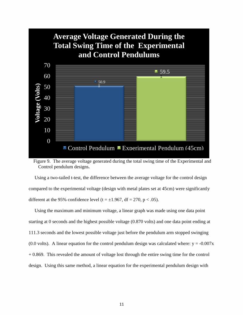
time, an average of 50.9 volts was created by the control method and 59.5 volts was created by

the experimental method with metal plates at 45cm from the pendulum arm (Figure 9).

11

Figure 9. The average voltage generated during the total swing time of the Experimental and

Control pendulum designs.

Using a two-tailed t-test, the difference between the average voltage for the control design

compared to the experimental voltage (design with metal plates set at 45cm) were significantly

different at the 95% confidence level (t = ±1.967, df = 270, p < .05).

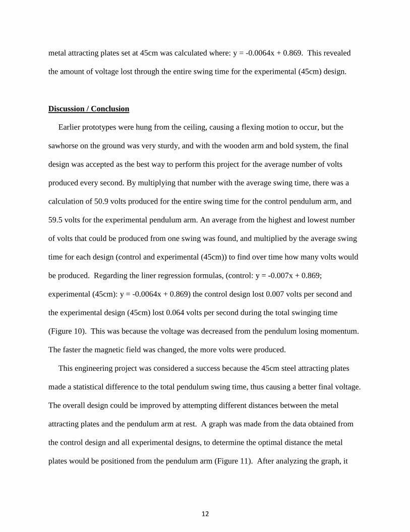
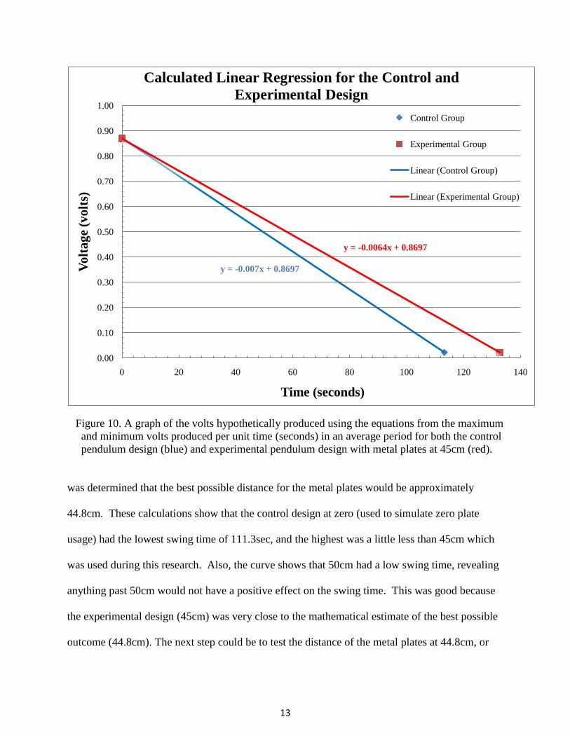
Using the maximum and minimum voltage, a linear graph was made using one data point

starting at 0 seconds and the highest possible voltage (0.870 volts) and one data point ending at

111.3 seconds and the lowest possible voltage just before the pendulum arm stopped swinging

(0.0 volts). A linear equation for the control pendulum design was calculated where: y = -0.007x

+ 0.869. This revealed the amount of voltage lost through the entire swing time for the control

design. Using this same method, a linear equation for the experimental pendulum design with

50.9

59.5

0

10

20

30

40

50

60

70

Vo

lta

ge

(Vo

lts)

Average Voltage Generated During the

Total Swing Time of the Experimental

and Control Pendulums

Control Pendulum Experimental Pendulum (45cm)

12

metal attracting plates set at 45cm was calculated where: y = -0.0064x + 0.869. This revealed

the amount of voltage lost through the entire swing time for the experimental (45cm) design.

Discussion / Conclusion

Earlier prototypes were hung from the ceiling, causing a flexing motion to occur, but the

sawhorse on the ground was very sturdy, and with the wooden arm and bold system, the final

design was accepted as the best way to perform this project for the average number of volts

produced every second. By multiplying that number with the average swing time, there was a

calculation of 50.9 volts produced for the entire swing time for the control pendulum arm, and

59.5 volts for the experimental pendulum arm. An average from the highest and lowest number

of volts that could be produced from one swing was found, and multiplied by the average swing

time for each design (control and experimental (45cm)) to find over time how many volts would

be produced. Regarding the liner regression formulas, (control: y = -0.007x + 0.869;

experimental (45cm): y = -0.0064x + 0.869) the control design lost 0.007 volts per second and

the experimental design (45cm) lost 0.064 volts per second during the total swinging time

(Figure 10). This was because the voltage was decreased from the pendulum losing momentum.

The faster the magnetic field was changed, the more volts were produced.

This engineering project was considered a success because the 45cm steel attracting plates

made a statistical difference to the total pendulum swing time, thus causing a better final voltage.

The overall design could be improved by attempting different distances between the metal

attracting plates and the pendulum arm at rest. A graph was made from the data obtained from

the control design and all experimental designs, to determine the optimal distance the metal

plates would be positioned from the pendulum arm (Figure 11). After analyzing the graph, it

13

Figure 10. A graph of the volts hypothetically produced using the equations from the maximum

and minimum volts produced per unit time (seconds) in an average period for both the control

pendulum design (blue) and experimental pendulum design with metal plates at 45cm (red).

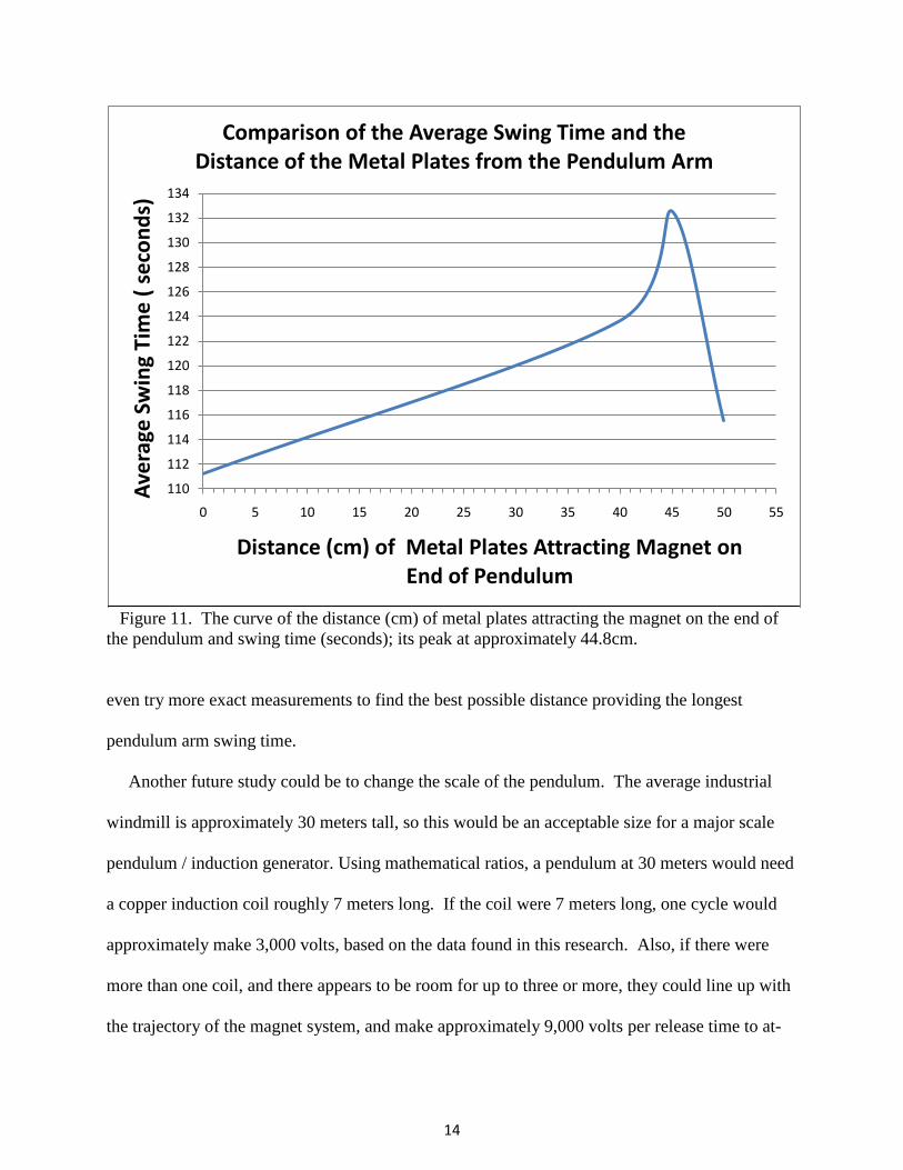
was determined that the best possible distance for the metal plates would be approximately

44.8cm. These calculations show that the control design at zero (used to simulate zero plate

usage) had the lowest swing time of 111.3sec, and the highest was a little less than 45cm which

was used during this research. Also, the curve shows that 50cm had a low swing time, revealing

anything past 50cm would not have a positive effect on the swing time. This was good because

the experimental design (45cm) was very close to the mathematical estimate of the best possible

outcome (44.8cm). The next step could be to test the distance of the metal plates at 44.8cm, or

y = -0.007x + 0.8697

y = -0.0064x + 0.8697

0.00

0.10

0.20

0.30

0.40

0.50

0.60

0.70

0.80

0.90

1.00

0 20 40 60 80 100 120 140

Vo

lta

ge

(vo

lts)

Time (seconds)

Calculated Linear Regression for the Control and

Experimental Design

Control Group

Experimental Group

Linear (Control Group)

Linear (Experimental Group)

14

Figure 11. The curve of the distance (cm) of metal plates attracting the magnet on the end of

the pendulum and swing time (seconds); its peak at approximately 44.8cm.

even try more exact measurements to find the best possible distance providing the longest

pendulum arm swing time.

Another future study could be to change the scale of the pendulum. The average industrial

windmill is approximately 30 meters tall, so this would be an acceptable size for a major scale

pendulum / induction generator. Using mathematical ratios, a pendulum at 30 meters would need

a copper induction coil roughly 7 meters long. If the coil were 7 meters long, one cycle would

approximately make 3,000 volts, based on the data found in this research. Also, if there were

more than one coil, and there appears to be room for up to three or more, they could line up with

the trajectory of the magnet system, and make approximately 9,000 volts per release time to at-

110

112

114

116

118

120

122

124

126

128

130

132

134

0 5 10 15 20 25 30 35 40 45 50 55

Ave

rage

Sw

ing

Tim

e (

se

con

ds)

Distance (cm) of Metal Plates Attracting Magnet on End of Pendulum

Comparison of the Average Swing Time and the Distance of the Metal Plates from the Pendulum Arm

15

rest time. If this magnet system was used, it would approximately make 71,000 kilo-volts per

day; theoretically in one year this would make 25,000 mega-volts. The pendulum generator

might have a building around itself, to protect from the elements and keep a constant temperature

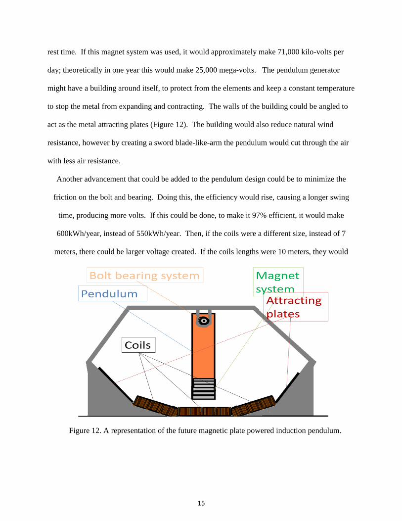
to stop the metal from expanding and contracting. The walls of the building could be angled to

act as the metal attracting plates (Figure 12). The building would also reduce natural wind

resistance, however by creating a sword blade-like-arm the pendulum would cut through the air

with less air resistance.

Another advancement that could be added to the pendulum design could be to minimize the

friction on the bolt and bearing. Doing this, the efficiency would rise, causing a longer swing

time, producing more volts. If this could be done, to make it 97% efficient, it would make

600kWh/year, instead of 550kWh/year. Then, if the coils were a different size, instead of 7

meters, there could be larger voltage created. If the coils lengths were 10 meters, they would

Figure 12. A representation of the future magnetic plate powered induction pendulum.

16

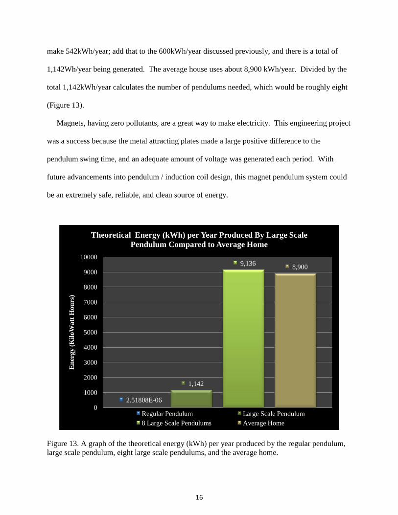
make 542kWh/year; add that to the 600kWh/year discussed previously, and there is a total of

1,142Wh/year being generated. The average house uses about 8,900 kWh/year. Divided by the

total 1,142kWh/year calculates the number of pendulums needed, which would be roughly eight

(Figure 13).

Magnets, having zero pollutants, are a great way to make electricity. This engineering project

was a success because the metal attracting plates made a large positive difference to the

pendulum swing time, and an adequate amount of voltage was generated each period. With

future advancements into pendulum / induction coil design, this magnet pendulum system could

be an extremely safe, reliable, and clean source of energy.

Figure 13. A graph of the theoretical energy (kWh) per year produced by the regular pendulum,

large scale pendulum, eight large scale pendulums, and the average home.

2.51808E-06

1,142

9,1368,900

0

1000

2000

3000

4000

5000

6000

7000

8000

9000

10000

En

ergy

(K

iloW

att

Hou

rs)

Theoretical Energy (kWh) per Year Produced By Large Scale

Pendulum Compared to Average Home

Regular Pendulum Large Scale Pendulum

8 Large Scale Pendulums Average Home

17

Acknowledgements

I would like to thank Jeff Wehr for financial and scientific support, and access to materials in

the laboratory. I would also like to thank Julie Wehr for helpful thinking and support. I would

like to thank Gary Smith for assisting in wood and metal working. I would like to thank the

Odessa School District for lab supplies and the data system probes.

Literature Cited & References

Collins, B. (2006). Interlinked Climate Challenges. The 21st century climate change comity.

Interlinked Climate Challenges. < http://colli239.fts.educ.msu.edu/wp-content/uploads/2009/07/co2emissions2000.jpg >,

(2/11/2010).

Davidson, M. (2006). Faraday's Magnetic Field Induction Experiment. National High Magnetic

Field Laboratory, Florida State University,

<http://micro.magnet.fsu.edu/electromag/java/faraday2/>, (1/24/2010).

Davis, S. (1999). Transportation Energy Data Book. Center for Transportation Analysis Energy

Division. Oak Ridge National Laboratory,

<http://ntl.bts.gov/lib/5000/5800/5844/19th_edition/Full_Doc_TEDB19.pdf>, (2/9/2010).

Hyper Physics Division. (2004). The Department of Physics and Astronomy. Georgia State

University, < http://hyperphysics.phy-astr.gsu.edu/HBASE/pend.html#c4 >, (2/10/2010).

Kumar, K. (1990). The national council of education research and training. Ministry of Human

Resources Development, Government of India,

< http://www.ncert.nic.in/html/learning_basket/electricity/images/electrostatics >, (2/11/2010).

Physics Van Outreach Program. (2010). University of Illinois Physics Department. Illinois

College of Engineering, Illinois State University, <http://van.physics.illinois.edu/index.html>,

(2/8/2010).

Russell, D. (2001). The simple pendulum :Small Angle Approximation and Simple Harmonic

Motion. Associate Professor of Applied Physics at Kettering University, Flint, MI

<http://paws.kettering.edu/~drussell/Demos.html>, (2/3/2010).