Projected Costs of Generating Electricity2015 Edition

Projected C

osts of Gen

erating Electricity – 2015 Ed

ition

Projected Costs of Generating Electricity

2015 Edition

INTERNATIONAL ENERGY AGENCY NUCLEAR ENERGY AGENCY

ORGANISATION FOR ECONOMIC CO-OPERATION AND DEVELOPMENT

INTERNATIONAL ENERGY AGENCY

The International Energy Agency (IEA), an autonomous agency, was established in November 1974. Its primary mandate was – and is – two-fold: to promote energy security amongst its member countries through collective response to physical disruptions in oil supply, and provide authoritative research and analysis on ways to ensure reliable, affordable and clean energy for its 29 member countries and beyond. The IEA carries out a comprehensive programme of energy co-operation among its member countries, each of which is obliged to hold oil stocks equivalent to 90 days of its net imports.

The Agency’s aims include the following objectives:

–  Secure member countries’ access to reliable and ample supplies of all forms of energy; in particular, through maintaining effective emergency response capabilities in case of oil supply disruptions.

–  Promote sustainable energy policies that spur economic growth and environmental protection in a global context – particularly in terms of reducing greenhouse-gas emissions that contribute to climate change.

–  Improve transparency of international markets through collection and analysis of energy data.

–  Support global collaboration on energy technology to secure future energy supplies and mitigate their environmental impact, including through improved energy efficiency and development and deployment of low-carbon technologies.

–  Find solutions to global energy challenges through engagement and dialogue with non-member countries, industry, international organisations and other stakeholders.

NUCLEAR ENERGY AGENCY

The OECD Nuclear Energy Agency (NEA) was established on 1 February 1958. Current NEA membership consists of 31 countries: Australia, Austria, Belgium, Canada, the Czech Republic, Denmark, Finland, France, Germany, Greece, Hungary, Iceland, Ireland, Italy, Japan, Korea, Luxembourg, Mexico, the Netherlands, Norway, Poland, Portugal, Russia, the Slovak Republic, Slovenia, Spain, Sweden, Switzerland, Turkey, the United Kingdom and the United States. The European Commission also takes part in the work of the Agency.

The mission of the NEA is:

–  to assist its member countries in maintaining and further developing, through international co-operation, the scientific, technological and legal bases required for a safe, environmentally friendly and economical use of nuclear energy for peaceful purposes;

–  to provide authoritative assessments and to forge common understandings on key issues, as input to government decisions on nuclear energy policy and to broader OECD policy analyses in areas such as energy and sustainable development.

Specific areas of competence of the NEA include the safety and regulation of nuclear activities, radioactive waste management, radiological protection, nuclear science, economic and technical analyses of the nuclear fuel cycle, nuclear law and liability, and public information.

The NEA Data Bank provides nuclear data and computer program services for participating countries. In these and related tasks, the NEA works in close collaboration with the International Atomic Energy Agency in Vienna, with which it has a Co-operation Agreement, as well as with other international organisations in the nuclear field.

ORGANISATION FOR ECONOMIC CO-OPERATION AND DEVELOPMENT

The OECD is a unique forum where the governments of 34 democracies work together to address the economic, social and environmental challenges of globalisation. The OECD is also at the forefront of efforts to understand and to help governments respond to new developments and concerns, such as corporate governance, the information economy and the challenges of an ageing population. The Organisation provides a setting where governments can compare policy experiences, seek answers to common problems, identify good practice and work to co-ordinate domestic and international policies.

The OECD member countries are: Australia, Austria, Belgium, Canada, Chile, the Czech Republic, Denmark, Estonia, Finland, France, Germany, Greece, Hungary, Iceland, Ireland, Israel, Italy, Japan, Korea, Luxembourg, Mexico, the Netherlands, New Zealand, Norway, Poland, Portugal, the Slovak Republic, Slovenia, Spain, Sweden, Switzerland, Turkey, the United Kingdom and the United States. The European Commission takes part in the work of the OECD.

OECD Publishing disseminates widely the results of the Organisation’s statistics gathering and research on economic, social and environmental issues, as well as the conventions, guidelines and standards agreed by its members.

Copyright © 2015 (30 September 2015 version)

Organisation for Economic Co-operation and Development/International Energy Agency 9, rue de la Fédération, 75739 Paris Cedex 15, France

and

Organisation for Economic Co-operation and Development/Nuclear Energy Agency 12, boulevard des Îles, 92130 Issy-les-Moulineaux, France

Please note that this publication is subject to specific restrictions that limit its use and distribution. The terms and conditions are available online at www.iea.org/t&c/

5

Foreword

Electricity is the fastest-growing final form of energy, and yet despite its increasing relevance to decarbonisation efforts, the future composition of the power sector remains uncertain. As policy makers work to ensure that the power sector is reliable and affordable, while making it increasingly clean and sustainable, it is ever more crucial that they understand what determines the relative cost of electricity generation using fossil fuel, nuclear or renewable technologies.

This eighth edition of Projected Costs of Generating Electricity, which examines in depth the levelised costs of electricity (LCOE) generation for all main electricity generating technologies, reveals a number of interesting findings that have implications for policy makers. Drawing on a database that includes a greater variety of technologies and a larger number of countries than previous editions, this report reaffirms many of the insights and lessons of the prior editions. The drivers of the cost of different generating technologies remain both market- and technology-specific. Low-carbon technologies remain highly capital intensive, and their overall cost depends significantly on the cost of capital. The relative cost of coal and natural gas-fired generation, meanwhile, is heavily contingent on fuel costs and, should such policies be fully implemented, the price of CO2 emissions.

One key trend that emerges is the significant decline in recent years in the cost of renewable generation as a result of the use of improved technologies and continued governmental support. The report also reveals that nuclear energy costs remain in line with the cost of other baseload technologies, despite persistent reports to the contrary. No single technology, however, can be said to be the cheapest under all circumstances. Rather, market structure, the policy environment and resource endowments all play a strong role in determining the final levelised cost of any given investment.

This study focuses on the LCOE metric because it remains valuable to policy makers for its relative simplicity and the ease with which it allows for comparability. Nevertheless, the relevance of LCOE in a world with liberalised power markets and increasing penetrations of variable renewable generation has been called into question. For the first time both the International Energy Agency (IEA) and the Nuclear Energy Agency (NEA) have worked together to try to address this question in a formal way.

This report is published under the responsibility of the IEA Executive Director, the NEA Director-General and the OECD Secretary-General. It reflects the collective views of the participating experts from OECD member and non-member countries, though not necessarily those of their parent organisations or governments.

6

Acknowledgements

The lead authors and co-ordinators of the report were Mr Matthew Wittenstein, Electricity Markets Analyst, IEA, and Dr Geoffrey Rothwell, Principal Economist, NEA. They would like to acknowledge the essential contribution of the Expert Group on Projected Costs of Generating Electricity (EGC Expert Group), which assisted in the sourcing of data, provided advice on methodological issues and reviewed successive drafts of the report. The group was chaired by Professor William D’haeseleer from Belgium and co-chaired by Mr Yuji Matsuo (Japan). Mr Laszlo Varro (IEA), Dr Paolo Frankl (IEA), Dr Manuel Baritaud (IEA) and Prof. Jan Horst Keppler (NEA) provided thoughtful advice and guidance.

Mr Matthew Wittenstein authored the chapters “Introduction and context”, “Technology overview”, “Country overview”, “Statistical analysis of key technologies” and “Sensitivity analysis”. Dr Geoffrey Rothwell authored the chapters “Methodology, conventions and key assumptions” and “Financing issues” and co-authored “History of projected costs of generating electricity, 1983-2015” with Ms Cyndia Yu, an NEA Consultant. Mr Marc Deffrennes (NEA), Dr Henri Paillère (NEA), Dr Uwe Remme (IEA) and Ms Cecilia Tam co-authored the chapter “Emerging generating technologies”. Mr Marco Cometto (NEA) and Mr Simon Mueller (IEA) co-authored the chapter “The system cost and system value of electricity generation”. Dr Manuel Baritaud (IEA) and Prof. Jan Horst Keppler (NEA) coauthored the chapter “Looking beyond baseload”. The report also benefited greatly from the work of Ms Cyndia Yu, who collected data on generating costs in the People’s Republic of China, and of Dr Noor Miza Muhamad Razali (IEA).

Ms Hélène Déry (NEA) and Ms Janet Pape (IEA) provided consistent and comprehensive administrative support.

7

Table of contents

Foreword ............................................................................................................................................................................................ 5

Acknowledgements .................................................................................................................................................................... 6

Table of contents .......................................................................................................................................................................... 7

List of tables .................................................................................................................................................................................... 9

List of figures .................................................................................................................................................................................. 11

Executive summary ................................................................................................................................................................... 13

PART I METHODOLOGY AND DATA ON LEVELISED COSTS FOR GENERATING TECHNOLOGIES

Chapter 1 Introduction and context ............................................................................................................................. 23

Chapter 2 Methodology, conventions and key assumptions ....................................................................... 27

2.1 The levelised cost of electricity ..................................................................................................... 27

2.2 Methodological conventions and key assumptions .......................................................... 30

2.3 Conclusions ............................................................................................................................................... 35

Chapter 3 Technology overview .................................................................................................................................... 37

3.1 Overview of different generating technologies .................................................................... 37

3.2 Technology-by-technology data on electricity generating costs .............................. 47

3.3 Capacity factor sensitivity of baseload technologies ....................................................... 56

Chapter 4 Country overview .............................................................................................................................................. 61

4.1 Country-by-country data on electricity generating costs (bar graphs) ................. 61

4.2 Country-by-country comparison of impact of capacity factor on LCOE .............. 85

4.3 Country-by-country data on electricity generating costs (numerical tables).... 90

Chapter 5 History of Projected Costs of Generating Electricity, 1981-2015 ......................................... 99

5.1 Introduction ............................................................................................................................................. 99

5.2 Previous editions .................................................................................................................................... 100

5.3 Country-by-country tables and figures on electricity generating costs for mainstream technologies.................................................................................................................. 102

8

PART II STATISTICAL AND SENSITIVITY ANALYSIS

Chapter 6 Statistical analysis of key technologies ............................................................................................. 111

6.1 The representative cost of renewable energy ..................................................................... 113

Chapter 7 Sensitivity analysis .......................................................................................................................................... 117

7.1 Multidimensional sensitivity analysis .................................................................................... 117

7.2 Detailed sensitivity analysis ........................................................................................................ 121

PART III BOUNDARY ISSUES

Chapter 8 Financing issues ................................................................................................................................................ 137

8.1 The social cost of capital versus private investment costs ........................................ 137

8.2 Private investment costs under uncertainty ....................................................................... 141

8.3 Questionnaire responses regarding the costs of capital and discount rates... 143

8.4 Options for improving investment conditions in the power sector...................... 145

Chapter 9 Emerging generating technologies ....................................................................................................... 147

9.1 High-efficiency, low-emission coal (IGCC and advanced-USC) ................................ 148

9.2 Carbon capture and storage ......................................................................................................... 149

9.3 Fuel cells ................................................................................................................................................... 150

9.4 Enhanced geothermal systems ................................................................................................... 151

9.5 Floating and deep offshore wind .............................................................................................. 152

9.6 Emerging solar photovoltaics ...................................................................................................... 153

9.7 Emerging solar thermal electricity (concentrating solar power) ........................... 154

9.8 Emerging bioenergy technologies ............................................................................................. 155

9.9 Ocean energy technologies ............................................................................................................ 156

9.10 Electricity storage technologies ................................................................................................. 157

9.11 Nuclear energy ..................................................................................................................................... 159

9.12 Concluding remarks ........................................................................................................................... 160

Chapter 10 The system cost and system value of electricity generation ................................................ 163

10.1 Going beyond generation costs ................................................................................................... 163

10.2 System effects ........................................................................................................................................ 165

10.3 System cost and system value .................................................................................................... 167

10.4 Long-term and short-term effects ............................................................................................ 170

10.5 Quantitative estimation of system effects ........................................................................... 177

10.6 Long-term transformation at growing shares of VRE .................................................... 180

Chapter 11 Looking beyond baseload: The future of the Projected Costs of Generating Electricity series ................................................................................................................................................. 185

11.1 Introduction ............................................................................................................................................ 185

11.2 The history and the future of the LCOE methodology: Usefulness and limitations ...................................................................................................................................... 186

11.3 The limits of LCOE in liberalised electricity markets with price risk ................... 187

11.4 New issues and new demands on power technologies in the presence of variable renewable energies .................................................................................................... 188

11.5 Four metrics of interest beyond levelised costs for future EGC studies ............. 190

11.6 Conclusions ............................................................................................................................................. 196

9

ANNEXES

Annex 1 The EGC spreadsheet model for calculating LCOE ...................................................................... 201

Annex 2 List of abbreviations and acronyms ...................................................................................................... 207

List of participating members of the EGC Expert Group ...................................................................................... 209

LIST OF TABLES

Table 1.1 Summary of responses by country and by technology .............................................................. 24

Table 2.1 National currency units per USD (2013 average) ............................................................................ 34

Table 3.1 Summary statistics for different generating technologies ..................................................... 37

Table 3.2 Natural gas-fired generating technologies ....................................................................................... 38

Table 3.3 Coal-fired generating technologies ....................................................................................................... 39

Table 3.4 Nuclear generating technologies ............................................................................................................ 41

Table 3.5 Solar generating technologies .................................................................................................................. 42

Table 3.6 Wind generating technologies ................................................................................................................. 44

Table 3.7 Other renewable generating technologies ........................................................................................ 45

Table 3.8 Combined heat and power technologies ........................................................................................... 46

Table 3.9 Levelised cost of electricity for natural gas plants ...................................................................... 48

Table 3.10 Levelised cost of electricity for coal plants ...................................................................................... 48

Table 3.11 Levelised cost of electricity for nuclear plants .............................................................................. 48

Table 3.12 Levelised cost of electricity for solar generators .......................................................................... 50

Table 3.13 Levelised cost of electricity for wind generators .......................................................................... 52

Table 3.14 Levelised cost of electricity for other renewable generation ................................................. 54

Table 3.15 Levelised cost of electricity for combined heat and power plants .................................... 56

Table 3.16 Levelised cost of electricity for combined-cycle gas turbines, 50% and 85% capacity factor ..................................................................................................................... 58

Table 3.17 Levelised cost of electricity for coal technologies, 50% and 85% capacity factor ..................................................................................................................... 58

Table 3.18 Levelised cost of electricity for nuclear technologies, 50% and 85% capacity factor ..................................................................................................................... 58

Table 4.1 Levelised costs of electricity for generating plants in Austria ............................................. 90

Table 4.2 Levelised costs of electricity for generating plants in Belgium ........................................... 91

Table 4.3 Levelised costs of electricity for generating plants in Denmark ......................................... 91

Table 4.4 Levelised costs of electricity for generating plants in Finland ............................................. 91

Table 4.5 Levelised costs of electricity for generating plants in France ............................................... 92

Table 4.6 Levelised costs of electricity for generating plants in Germany ......................................... 92

Table 4.7 Levelised costs of electricity for generating plants in Hungary .......................................... 93

Table 4.8 Levelised costs of electricity for generating plants in Italy .................................................... 93

Table 4.9 Levelised costs of electricity for generating plants in Japan ................................................. 93

Table 4.10 Levelised costs of electricity for generating plants in Korea .................................................. 94

Table 4.11 Levelised costs of electricity for generating plants in the Netherlands ......................... 94

Table 4.12 Levelised costs of electricity for generating plants in New Zealand ................................ 94

Table 4.13 Levelised costs of electricity for generating plants in Portugal ........................................... 95

10

Table 4.14 Levelised costs of electricity for generating plants in the Slovak Republic .................. 95

Table 4.15 Levelised costs of electricity for generating plants in Spain ................................................. 95

Table 4.16 Levelised costs of electricity for generating plants in Switzerland ................................... 96

Table 4.17 Levelised costs of electricity for generating plants in Turkey ............................................... 96

Table 4.18 Levelised costs of electricity for generating plants in the United Kingdom ................ 96

Table 4.19 Levelised costs of electricity for generating plants in the United States ....................... 97

Table 4.20 Levelised costs of electricity for generating plants in Brazil ................................................. 98

Table 4.21 Levelised costs of electricity for generating plants in China ................................................ 98

Table 4.22 Levelised costs of electricity for generating plants in South Africa .................................. 98

Table 5.1a Historical LCOE data, 5% discount rate (2013 USD/MWh) – natural gas (CCGT) ....... 103

Table 5.1b Historical LCOE data, 10% discount rate (2013 USD/MWh) – natural gas (CCGT) ..... 103

Table 5.2a Historical LCOE data, 5% discount rate (2013 USD/MWh) – coal ......................................... 104

Table 5.2b Historical LCOE data, 10% discount rate (2013 USD/MWh) – coal ...................................... 104

Table 5.3a Historical LCOE data, 5% discount rate (2013 USD/MWh) – nuclear ................................. 105

Table 5.3b Historical LCOE data, 10% discount rate (2013 USD/MWh) – nuclear ............................... 105

Table 6.1 Overview of data for natural gas generation ................................................................................... 111

Table 6.2 Overview of data for coal generation ................................................................................................... 111

Table 6.3 Overview of data for nuclear generation ........................................................................................... 112

Table 6.4 Overview of data for residential solar PV generation ................................................................ 112

Table 6.5 Overview of data for commercial solar PV generation ............................................................. 112

Table 6.6 Overview of data for large ground-mounted solar PV generation ..................................... 112

Table 6.7 Overview of data for onshore wind generation ............................................................................. 113

Table 8.1 Nominal and real yields on government ten-year bonds, March 2015............................. 139

Table 8.2 Questionnaire responses regarding the costs of capital .......................................................... 144

Table 9.1 Technical and economic characteristics for A-USC and IGCC technologies in 2030 .. 148

Table 9.2 Technical and economic characteristics for CCS technologies in 2030 .......................... 149

Table 9.3 Technical and economic characteristics for FC technologies in 2030 ............................. 151

Table 9.4 LCOE for EGS technologies in 2030 ........................................................................................................ 152

Table 9.5 LCOE for floating and deep offshore wind technologies in 2015 and 2030 ................... 153

Table 9.6 LCOE for solar PV in 2015 and 2030 ....................................................................................................... 154

Table 9.7 LCOE for CSP with storage in 2015 and 2030 ................................................................................... 155

Table 9.8 LCOE for bioenergy technologies in 2015 and 2030 ..................................................................... 156

Table 9.9 LCOE for ocean technologies in 2020 and 2030 .............................................................................. 157

Table 9.10 Technical and economic characteristics for electricity storage technologies ............ 158

Table 9.11 Technical and economic characteristics for emerging nuclear technologies ............. 160

Table 9.12 Cost summary of LTO and refurbishment programmes in selected countries .......... 161

Table 11.1 Capability of different power generating technologies to provide flexibility .............. 193

Table A2.1 National currency units per USD (2013 average) ......................................................................... 202

11

LIST OF FIGURES

Figure ES.1 LCOE ranges for baseload technologies (at each discount rate) ........................................... 14

Figure ES.2 LCOE ranges for solar PV and wind technologies (at each discount rate) ...................... 15

Figure ES.3 EGC 2010 and EGC 2015 LCOE ranges for baseload technologies (at 10% discount rate) ..................................................................................................................................... 18

Figure ES.4 EGC 2010 and EGC 2015 LCOE ranges for solar and wind technologies (at 10% discount rate) ..................................................................................................................................... 18

Figure 4.1 Levelised cost of electricity – Austria ................................................................................................... 62

Figure 4.2 Levelised cost of electricity – Belgium ................................................................................................. 63

Figure 4.3 Levelised cost of electricity – Denmark .............................................................................................. 64

Figure 4.4 Levelised cost of electricity – Finland .................................................................................................. 65

Figure 4.5 Levelised cost of electricity – France .................................................................................................... 66

Figure 4.6 Levelised cost of electricity – Germany .............................................................................................. 67

Figure 4.7 Levelised cost of electricity – Hungary ................................................................................................ 68

Figure 4.8 Levelised cost of electricity – Italy ......................................................................................................... 69

Figure 4.9 Levelised cost of electricity – Japan ...................................................................................................... 70

Figure 4.10 Levelised cost of electricity – Korea ...................................................................................................... 71

Figure 4.11 Levelised cost of electricity – Netherlands ....................................................................................... 72

Figure 4.12 Levelised cost of electricity – New Zealand ..................................................................................... 73

Figure 4.13 Levelised cost of electricity – Portugal ................................................................................................ 74

Figure 4.14 Levelised cost of electricity – Slovak Republic ................................................................................ 75

Figure 4.15 Levelised cost of electricity – Spain ...................................................................................................... 76

Figure 4.16 Levelised cost of electricity – Switzerland ........................................................................................ 77

Figure 4.17 Levelised cost of electricity – Turkey .................................................................................................... 78

Figure 4.18 Levelised cost of electricity – United Kingdom .............................................................................. 79

Figure 4.19 Levelised cost of electricity – United States – Nuclear, fossil and biomass technologies .................................................................................................................................... 80

Figure 4.19 Levelised cost of electricity – United States – Other renewable technologies ............ 81

Figure 4.20 Levelised cost of electricity – Brazil ...................................................................................................... 82

Figure 4.21 Levelised cost of electricity – China ...................................................................................................... 83

Figure 4.22 Levelised cost of electricity – South Africa ....................................................................................... 84

Figure 4.23 LCOE at 85% and 50% capacity factor – Belgium (7% discount rate) .................................. 85

Figure 4.24 LCOE at 85% and 50% capacity factor – Finland (7% discount rate).................................... 85

Figure 4.25 LCOE at 85% and 50% capacity factor – France (7% discount rate) ...................................... 86

Figure 4.26 LCOE at 85% and 50% capacity factor – Germany (7% discount rate) ................................ 86

Figure 4.27 LCOE at 85% and 50% capacity factor – Hungary (7% discount rate) ................................. 86

Figure 4.28 LCOE at 85% and 50% capacity factor – Japan (7% discount rate) ........................................ 87

Figure 4.29 LCOE at 85% and 50% capacity factor – Korea (7% discount rate) ........................................ 87

Figure 4.30 LCOE at 85% and 50% capacity factor – Netherlands (7% discount rate) ......................... 87

Figure 4.31 LCOE at 85% and 50% capacity factor – New Zealand (7% discount rate) ....................... 88

Figure 4.32 LCOE at 85% and 50% capacity factor – Portugal (7% discount rate) .................................. 88

Figure 4.33 LCOE at 85% and 50% capacity factor – Slovak Republic (7% discount rate) ................. 88

Figure 4.34 LCOE at 85% and 50% capacity factor – United Kingdom (7% discount rate) ............... 89

Figure 4.35 LCOE at 85% and 50% capacity factor – United States (7% discount rate) ...................... 89

Figure 4.36 LCOE at 85% and 50% capacity factor – China (7% discount rate) ....................................... 89

12

Figure 4.37 LCOE at 85% and 50% capacity factor – South Africa (7% discount rate) ......................... 90

Figure 5.1 Historical LCOE results for OECD countries – CCGTs ................................................................. 106

Figure 5.2 Historical LCOE results for OECD countries – coal ....................................................................... 107

Figure 5.3 Historical LCOE results for OECD countries – nuclear ............................................................... 108

Figure 6.1 LCOEs for utility-scale solar PV, by project, 2013 and 2014 ..................................................... 114

Figure 6.2 Utility-scale solar PV LCOEs projected in 2020 .............................................................................. 115

Figure 7.1 Tornado charts – natural gas (CCGT) .................................................................................................... 118

Figure 7.2 Tornado charts – coal ..................................................................................................................................... 119

Figure 7.3 Tornado charts – nuclear ............................................................................................................................. 119

Figure 7.4 Tornado charts – solar PV, commercial rooftop ............................................................................. 120

Figure 7.5 Tornado charts – onshore wind ............................................................................................................... 121

Figure 7.6 LCOE as a function of the discount rate ............................................................................................. 122

Figure 7.7 Ratio of investment cost to total cost as a function of discount rate .............................. 123

Figure 7.8 LCOE as a function of overnight cost ................................................................................................... 124

Figure 7.9 LCOE as a function of construction lead time ................................................................................ 125

Figure 7.10 LCOE of coal, natural gas and nuclear as a function of capacity factor ......................... 127

Figure 7.11 LCOE as a function of lifetime .................................................................................................................. 129

Figure 7.12 LCOE as a function of fuel cost ................................................................................................................ 131

Figure 7.13 Ratio of fuel cost to total LCOE ................................................................................................................ 132

Figure 7.14 LCOE as a function of carbon price ....................................................................................................... 133

Figure 8.1 Nominal and real yields on US Treasuries, April 2015 ............................................................... 138

Figure 8.2 Nominal yields on Japanese government ten-year bonds, 2007-2014 ............................. 139

Figure 8.3 Standard and Poor’s government bond ratings ............................................................................. 140

Figure 10.1 Illustration of system costs, system value and system cost approaches ...................... 168

Figure 10.2 Illustration of the relationship between system value and system costs for wind power and benchmark technology ................................................................................... 169

Figure 10.3 Short-term reduction in capacity factor for existing power plants after the introduction of wind power .............................................................................................................. 172

Figure 10.4 Illustration of the merit order effect .................................................................................................... 173

Figure 10.5 Optimal long-term generation mix with and without VRE .................................................... 175

Figure 10.6 Illustration of capacity credit evolution after increasing share of solar PV generation ................................................................................................................................... 176

Figure 10.7 Comparison of modelled balancing costs from different integration studies ............ 179

Figure 11.1 Power sector investment, 2014-2035 .................................................................................................... 187

Figure 11.2 Levelised cost of capacity, median case, USD/kW ........................................................................ 192

Figure 11.3 Value factor of wind power ........................................................................................................................ 195

13

Executive summary

Projected Costs of Generating Electricity – 2015 Edition is the eighth report in the series on the levelised costs of generating electricity. This report presents the results of work performed in 2014 and early 2015 to calculate the cost of generating electricity for both baseload electricity generated from fossil fuel thermal and nuclear power stations, and a range of renewable generation, including variable sources such as wind and solar. It is a forward-looking study, based on the expected cost of commissioning these plants in 2020.

The LCOE calculations are based on a levelised average lifetime cost approach, using the discounted cash flow (DCF) method. The calculations use a combination of generic, country-specific and technology-specific assumptions for the various technical and economic parameters, as agreed by the Expert Group on Projected Costs of Generating Electricity (EGC Expert Group). For the first time, the analysis was performed using three discount rates (3%, 7% and 10%).1

Costs are calculated at the plant level (busbar), and therefore do not include transmission and distribution costs. Similarly, the LCOE calculation does not capture other systemic costs or externalities beyond CO2 emissions.2

The analysis within this report is based on data for 181 plants in 22 countries (including 3 non-OECD countries3). This total includes 17 natural gas-fired generators (13 combined-cycle gas turbines [CCGTs] and 4 open-cycle gas turbines [OCGTs]), 14 coal plants,4 11 nuclear power plants, 38 solar photovoltaic (PV) plants (12 residential scale, 14 commercial scale, and 12  large, ground-mounted) and 4 solar thermal (CSP) plants, 21 onshore wind plants, 12 offshore wind plants, 28 hydro plants, 6 geothermal, 11 biomass and biogas plants and 19 combined heat and power (CHP) plants of varying types. This data set contains a marked shift in favour of renewables compared to the prior reports, indicating an increased interest in low-carbon technologies on the part of the participating governments.

Part II of the study contains statistical analysis of the underlying data (including a focused analysis on the cost of renewables) and a sensitivity analysis. Part III contains discussions of “boundary issues” that do not necessarily enter into the calculation of LCOEs, but have an impact on decision making in the electricity sector. The chapter on financing focuses on issues affecting the cost of capital, a key topic given the trends noted above. The chapter on emerging generating technologies provides a glimpse of what the next study may include, as these emerging technologies are commercialised. The final two chapters present cost issues from a system perspective and cost metrics that may, in addition to LCOE, provide deeper insight into the true cost of technologies in liberalised markets with high penetrations of variable renewable power.

1. See Chapter 2 on “Methodology, conventions and key assumptions” for further details on questions of methodology and Chapter 8 on “Financing issues” for a discussion of discount rates. To aid in comparability with prior studies, results for a discount rate of 5% are presented in Chapter 5, “History of Projected Costs of Generating Electricity, 1981-2015”.

2. The report does not attempt to calculate the impact of CO2 emissions or non-monetarised externalities associated with fossil-fired plants (e.g. in their fuel production) or with nuclear power plants (e.g. in their fuel cycles).

3. Brazil, China and South Africa.

4. Contrary to the 2010 study, plants with carbon capture and storage (CCS) were excluded from this analysis.

14

Results

Figure ES.1 shows the range of LCOE results for the three baseload technologies analysed in this report (natural gas-fired CCGTs, coal and nuclear). At a 3% discount rate, nuclear is the lowest cost option for all countries. However, consistent with the fact that nuclear technologies are capital intensive relative to natural gas or coal, the cost of nuclear rises relatively quickly as the discount rate is raised. As a result, at a 7% discount rate the median value of nuclear is close to the median value for coal, and at a 10% discount rate the median value for nuclear is higher than that of either CCGTs or coal. These results include a carbon cost of USD 30/tonne, as well as regional variations in assumed fuel costs.

Figure ES.1: LCOE ranges for baseload technologies (at each discount rate)

LCO

E (U

SD/M

Wh)

0

20

40

60

80

100

120

140

160

NuclearCoalCCGTNuclearCoalCCGTNuclearCoalCCGT

Median

3% 7% 10%

The ranges presented include results from all countries analysed in this study, and therefore obscure regional variations. For a more granular analysis, see Chapter 3 on “Technology overview”.

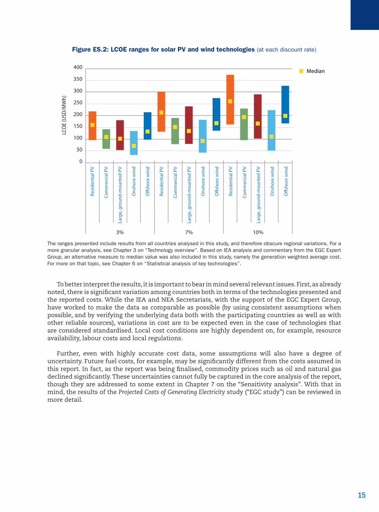
Figure ES.2 shows the LCOE ranges for various renewable technologies – namely, the three categories of solar PV in the study (residential, commercial and large, ground-mounted) and the two categories of wind (onshore and offshore). It is immediately apparent that the ranges in costs are significantly larger than for baseload technologies. It is also notable that the costs across technologies are relatively in line with one another. While at the high end, the LCOE for renewable technologies remains well above those of baseload technologies, at the low-end costs are in line with – or even below – baseload technologies. Solar PV in particular has seen significant declines in cost since the previous study, though onshore wind remains the lowest cost renewable technology. The median values for these technologies are, for the most part, closer to the low end of the range, a reflection of the fact that this chart obscures significant regional variations in costs (in particular for solar PV). This is not surprising, because the cost of renewable technologies is determined in large part by local resource availability, which can vary significantly among countries or even within countries.

15

Figure ES.2: LCOE ranges for solar PV and wind technologies (at each discount rate)

LCO

E (U

SD/M

Wh)

0

50

100

150

200

250

300

350

400Median

3% 7% 10%

O�s

hore

win

d

Ons

hore

win

d

Larg

e, g

roun

d-m

ount

ed P

V

Com

mer

cial

PV

Resi

dent

ial P

V

O�s

hore

win

d

Ons

hore

win

d

Larg

e, g

roun

d-m

ount

ed P

V

Com

mer

cial

PV

Resi

dent

ial P

V

O�s

hore

win

d

Ons

hore

win

d

Larg

e, g

roun

d-m

ount

ed P

V

Com

mer

cial

PV

Resi

dent

ial P

V

The ranges presented include results from all countries analysed in this study, and therefore obscure regional variations. For a more granular analysis, see Chapter 3 on “Technology overview”. Based on IEA analysis and commentary from the EGC Expert Group, an alternative measure to median value was also included in this study, namely the generation weighted average cost. For more on that topic, see Chapter 6 on “Statistical analysis of key technologies”.

To better interpret the results, it is important to bear in mind several relevant issues. First, as already noted, there is significant variation among countries both in terms of the technologies presented and the reported costs. While the IEA and NEA Secretariats, with the support of the EGC Expert Group, have worked to make the data as comparable as possible (by using consistent assumptions when possible, and by verifying the underlying data both with the participating countries as well as with other reliable sources), variations in cost are to be expected even in the case of technologies that are considered standardised. Local cost conditions are highly dependent on, for example, resource availability, labour costs and local regulations.

Further, even with highly accurate cost data, some assumptions will also have a degree of uncertainty. Future fuel costs, for example, may be significantly different from the costs assumed in this report. In fact, as the report was being finalised, commodity prices such as oil and natural gas declined significantly. These uncertainties cannot fully be captured in the core analysis of the report, though they are addressed to some extent in Chapter 7 on the “Sensitivity analysis”. With that in mind, the results of the Projected Costs of Generating Electricity study (“EGC study”) can be reviewed in more detail.

16

Baseload technologies

Overnight costs for natural gas-fired CCGTs in OECD countries range from USD 845/kWe (Korea) to USD 1 289/kWe (New Zealand). In LCOE terms, costs at a 3% discount rate range from a low of USD 61/MWh in the United States to USD 133/MWh in Japan. The United States has the lowest cost CCGT in LCOE terms, despite having a relatively high capital cost, which demonstrates the significant impact that variations in fuel price can have on the final cost. At a 7% discount rate, LCOEs range from USD 66/MWh (United States) to USD 138/MWh (Japan), and at a 10% discount rate they range from USD 71/MWh (United States) to USD 143/MWh (Japan).

Overnight costs for coal plants in OECD countries range from a low of USD 1 218/kWe in Korea to a high of USD 3 067/kWe in Portugal. In OECD countries, LCOEs at a 3% discount rate range from a low of USD 66/MWh in Germany to a high of USD 95/MWh in Japan. At a 7% discount rate, LCOEs range from USD 76/MWh (Germany) to USD 107/MWh (Japan), and at a 10% discount rate they range from USD 83/MWh (Germany) to USD 119/MWh (Japan).

The range of overnight costs for nuclear technologies in OECD countries is large, from a low of USD 2 021/kWe in Korea to a high of USD 6 215/kWe in Hungary. LCOEs at a 3% discount rate range from USD 29/MWh in Korea to USD 64/MWh in the United Kingdom, USD 40/MWh (Korea) to USD 101/MWh (United Kingdom) at a 7% discount rate and USD 51/MWh (Korea) to USD 136/MWh (United Kingdom) at 10%.

Solar PV and wind technologies

Solar PV technologies are divided into three categories: residential, commercial, and large, ground-mounted. Overnight costs for residential PV range from USD 1 867/kWe in Portugal to USD 3 366/kWe in France.5 LCOEs at a 3% discount rate range from USD 96/MWh in Portugal to USD 218/MWh in Japan. At a 7% discount rate, LCOEs range from USD 132/MWh in Portugal to USD 293/MWh in France. At a 10% discount rate, they range from USD 162/MWh to USD 374/MWh, in Portugal for both cases.

For commercial PV, overnight costs range from USD 1 029/kWe in Austria to USD 1 977/kWe in Denmark. LCOEs range from USD 69/MWh in Austria to USD 142/MWh in Belgium at a 3% discount rate, USD 98/MWh (Austria) to USD 190/MWh (Belgium) at a 7% discount rate and USD 121/MWh (Portugal) to USD 230/MWh (Belgium) at a 10% discount rate.

Overnight costs for large, ground-mounted PV range from USD  1  200/kWe in Germany to USD 2 563/kWe in Japan. LCOEs at a 3% discount rate range from USD 54/MWh in the United States to USD 181/MWh in Japan, USD 80/MWh (United States) to USD 239/MWh (Japan) at a 7% discount rate and USD 103/MWh (United States) to USD 290/MWh (Japan) at a 10% discount rate.

Onshore wind plant overnight costs range from USD 1 571/kWe in the United States to USD 2 999/kWe in Japan. At a 3% discount rate, LCOEs range from USD 33/MWh in the United States to USD 135/MWh in Japan, USD  43/MWh (United States) to USD  182/MWh (Japan) at a 7% discount rate and USD 52/MWh (United States) to USD 223/MWh at a 10% rate (Japan).

Finally, overnight costs for offshore wind plants range from USD 3 703/kWe in the United Kingdom to USD 5 933/kWe in Germany. LCOEs at a 3% discount rate range from USD 98/MWh in Denmark to USD 214/MWh in Korea; at a 7% discount rate, they range from USD 136/MWh (Denmark) to USD 275/MWh (Korea); and at a 10% discount rate, they range from USD 167/MWh (United States) to USD 327/MWh (Korea).

5. Costs in France, for residential rooftop, include additional costs specific to roof-integrated solar systems.

17

Results from non-OECD countries

The study also includes data from three non-OECD countries: Brazil (hydro only), the People’s Republic of China and South Africa. In the particular case of China, data was derived from a combination of publicly available sources and survey data – in particular, the IEA Photovoltaic Power Systems Programme (PVPS) survey. They cannot, therefore, be considered official data from China for the Projected Costs of Generating Electricity study. Nevertheless, it is important to consider the possible costs of generation in China as part of this study.

The estimated overnight cost for a CCGT in China (the only non-OECD data point in the sample) is USD 627/kWe, while the LCOE is USD 90/MWh, USD 93/MWh and USD 95/MWh at 3%, 7%, and 10% discount rates respectively. For coal, cost estimates are included for China, with an overnight cost of USD 813/kWe, and South Africa, with an overnight cost of USD 2 222/kWe. The LCOEs for China are USD 74/MWh at a 3% discount rate, USD 78/MWh at a 7% discount rate and USD 82/MWh at a 10% discount rate. For South Africa, the range is larger: USD 65/MWh at 3%, USD 82/MWh at 7% and USD 100/MWh at 10%. The report includes two nuclear data points for China, with overnight costs of USD 1 807/kWe and USD 2 615/kWe; LCOES are USD 26/MWh and USD 31/MWh at a 3% discount rate, USD 37/MWh and USD 48/MWh at 7% and USD 49/MWh and USD 64/MWh at 10%.

For solar PV, China has the lowest cost commercial PV plant in the database, with an overnight cost of USD  728/kWe; LCOEs are USD  59/MWh, USD  78/MWh and USD  96/MWh at 3%, 7% and 10% discount rates respectively. The overnight cost for the large, ground-mounted PV plant is USD  937/kWe; the LCOEs are USD  55/MWh, USD  73/MWh and USD  88/MWh at 3%, 7% and 10% discount rates. Finally, for onshore wind, overnight costs for the two estimates from China are USD 1 200/kWe and USD 1 400/kWe. While in South Africa, the single onshore wind plant in the database is USD 2 756/kWe; LCOEs are USD 77/MWh, USD 102/MWh and USD 123/MWh at 3%, 7% and 10% respectively.

Details on other technologies included in the report, such as OCGTs, solar thermal, hydro, biomass/biogas and CHPs can be found in Chapters 3 and 4.

Comparison with EGC 2010

While changes in assumptions and differences both in terms of size and composition of the underlying dataset make cross-study comparisons difficult, it is nevertheless useful to examine, at a high-level, how cost estimates have changed over time.6 Figure ES.3 compares the range of LCOE results for baseload technologies in the most recent 2010 edition of Projected Costs of Generating Electricity (EGC 2010) and in the current study.

The EGC 2010 results show a wider range of LCOEs, in particular for coal-fired generation. This is in part due to the fact that EGC 2010 contained a greater number of data points for each technology than there are in EGC 2015,7 but also because of changes in fuel price and other underlying assumptions. While the range of LCOE values is smaller in EGC 2015, it is notable that the median value for each technology is higher than in EGC 2010. While the median value is an imprecise measurement for comparing costs between technology categories and across countries, the fact that the median value is higher in each case does suggest the possibility of increasing costs for each of these technologies on an LCOE basis.

6. For a more detailed examination of the history of the Projected Costs of Generating Electricity study, see Chapter 5.

7. EGC 2010 contained 23 CCGTs (without CCS), 31 coal-fired plants (without CCS), and 20 nuclear power plants, compared to 13 CCGTs, 14 coal-fired plants and 11 nuclear plants in EGC 2015.

18

Figure ES.3: EGC 2010 and EGC 2015 LCOE ranges for baseload technologies (at 10% discount rate)

LCO

E (U

SD/M

Wh)

Median

CCGT Coal Nuclear

0

20

40

60

80

100

120

140

160

EGC 2015EGC 2010EGC 2015EGC 2010EGC 2015EGC 2010

* EGC 2010 results have been converted to USD 2013 values for comparison.

For renewable technologies (specifically, solar PV and onshore wind), the change relative to EGC 2010 is in the opposite direction. This can be seen most clearly in the LCOE values for solar PV, where, despite a larger number of data points in EGC 2015,8 there are both a smaller range of LCOE values and a very significant decline in costs. Onshore wind LCOEs are also noticeably lower in EGC 2015, though the difference is much less pronounced.9

Figure ES.4: EGC 2010 and EGC 2015 LCOE ranges for solar and wind technologies (at 10% discount rate)

LCO

E (U

SD/M

Wh)

Median

Solar PV(all technologies) Onshore wind

0

200

400

600

800

1 000

1 200

EGC 2015EGC 2010EGC 2015EGC 2010

* EGC 2010 results have been converted to USD 2013 values for comparison.

8. EGC 2010 contained 17 solar PV technologies, compared to 38 in EGC 2015.

9. The median value presented in these figures may not fully represent renewable energy costs, as it gives equal weight to markets or data points which may be less relevant globally. For a more detailed discussion on the cost of renewable energy – and, in particular an alternative measurement to the median value – see Section 6.1 of the report.

19

Conclusions

This eighth edition of Projected Costs of Generating Electricity focuses on the cost of generation for a limited set of countries, and even within these countries only for a subset of technologies. Caution must therefore be taken when attempting to derive broad lessons from the analysis. Nevertheless, some conclusions can be drawn.

First, the vast majority of the technologies included in this study are low- or zero-carbon sources, suggesting a clear shift in the interest of participating countries away from fossil-based technologies, at least as compared to the 2010 study.

Second, while the 2010 study noted a significant increase in the cost of baseload technologies, the data in this report suggest that any such cost inflation has been arrested. This is particularly notable in the case of nuclear technologies, which have costs that are roughly on a par with those reported in the prior study, thus undermining the growing narrative that nuclear costs continue to increase globally.

Finally, this report clearly demonstrates that the cost of renewable technologies – in particular solar photovoltaic – have declined significantly over the past five years, and that these technologies are no longer cost outliers.

Despite the general relevance of these conclusions, the cost drivers of the different generating technologies nonetheless remain both market- and technology-specific. As such, there is no single technology that can be said to be the cheapest under all circumstances. As this edition of the study makes clear, system costs, market structure, policy environment and resource endowment all continue to play an important role in determining the final levelised cost of any given investment.

Part 1Methodology and data on levelised costs

for generating technologies

23

1

23

Chapter

Introduction and context

This is the eighth edition of the report on Projected Costs of Generating Electricity, a joint project of the International Energy Agency (IEA) and the Nuclear Energy Agency (NEA), also referred to as the report on Electricity Generating Costs (EGC) 2015. The seventh edition was published in 2010 (EGC 2010). As with previous editions, this report relies on contributions from both OECD and non-OECD countries. In addition, an expert group composed of country and industry representatives provided key advice on methodology, data collection, and on the content and format of this report.

The core of the report is an analysis of the levelised cost of electricity (LCOE) in 22 countries across multiple generating technologies and fuels. This report recognises that LCOE is both an important tool for comparing generating technologies, but also that the underlying data are of interest to its many readers. For that reason, the energy cost components and the LCOE have been presented as transparently as possible in Part I. In addition, and in keeping with the precedent EGC 2010 set, a detailed sensitivity analysis is included (Part II), as well as a set of chapters examining topics that are relevant to, but not captured by, the LCOE analysis itself (Part III).

The set of countries included in this updated report is broadly consistent with the countries included in EGC 2010. The IEA and NEA jointly invited government representatives of OECD member countries, and a select group of non-OECD countries, to submit data for use in this updated study. Countries participated on a voluntary basis, and while some countries elected not to submit data this time, a number of additional countries are included in this study that were not included in the 2010 report. The result is a dataset that offers a diversity of both countries and technologies, and that is broadly representative of the state of electric power generation development today. In total, the EGC 2015 database contains 181 data points from 22 countries. A summary of participating countries and technologies can be found in Table 1.1.

As with previous studies, most data were either provided by member country governments directly or by experts nominated by those countries to participate in the EGC Expert Group. (The main exception is China, where data were collected from a variety of public sources.) The methodology employed is, to an extent deemed reasonable, consistent with that of EGC 2010. Assumptions have been reviewed and updated as appropriate to reflect the current state of the electricity sector globally. In all cases, the methodology and assumptions have been vetted by the members of the expert group.

This series of studies on electricity generating costs has proven to be an important tool for policy makers, academics, and the interested public when discussing the economics of power generation. It is therefore important to provide the context in which the work has been completed.

As noted in EGC 2010, there is significant uncertainty as to the underlying drivers of generating costs, and again this study includes a broad range of costs for technologies even when comparing countries that are expected to be relatively similar. The 2010 report noted five potential explanations for this uncertainty: privatisation, market liberalisation and related limitations on the public availability of data; policy uncertainty; the evolution of generating technologies; lack of recent construction within OECD countries; and rapid changes in power plant costs. It is worth revisiting them to examine the degree to which these explanations remain relevant.

24

1

24

Table 1.1: Summary of responses by country and by technology

Country Natural gas Coal Nuclear Solar

PVSolar

thermalOnshore

windOffshore

wind Hydro CHP Other Total

Austria 1 1 1 2 5Belgium 2 1 1 2 1 1 8Denmark 3 1 1 6 11Finland 1 1France 1 1 3 1 1 7Germany 2 2 3 1 1 2 5 16Hungary 1 1 3 1 6Italy 3 1 1 4 9Japan 1 1 1 2 1 1 7Korea 2 2 1 3 1 1 10Netherlands 1 3 1 1 1 2 2 11New Zealand 2 1 1 4Portugal 1 2 3 1 1 2 10Slovak Republic 1 1Spain 3 1 1 4 2 4 15Switzerland 1 4 5Turkey 1 1 1 3United Kingdom 2 1 2 1 2 1 2 2 13United States 1 1 1 3 2 3 3 6 3 23

Non-OECD countries

Brazil 4 4China* 1 1 2 2 2 1 9South Africa 1 1 1 3TOTAL 17 14 11 38 4 21 12 28 19 17 181

* China did not provide an official response to the EGC questionnaire. Data was instead drawn from various public sources and surveys.

First, the privatisation of utilities, and, more broadly, electric power market liberalisation within OECD markets, has reduced the public availability of some cost data. Confidentiality and competitiveness concerns remain an issue, because the desire to maintain a competitive edge by project sponsors and equipment manufacturers reduces the willingness of those parties to share detailed cost information. This is in particular the case for technologies that are considered sensitive, such as nuclear power. This issue has seemingly increased in relevance, as industrial companies or industry groups only contributed data to EGC 2015 through the relevant member governments.

Second, policy uncertainty remains a limitation in projecting future operating costs, in particular in the area of climate change. In keeping with the methodology adopted for EGC 2010, a cost for carbon dioxide (CO2) was included in US dollars (USD) 30/tonne. This assumption is maintained despite the fact that CO2 prices in general remain low or, in some countries, entirely absent. Including a price of USD 30/tonne in this report acknowledges that a carbon price remains a topic of discussion among policy makers globally, and also affords a degree of comparability between this report and EGC 2010. Part II examines, inter alia, the sensitivity of relevant technologies to the cost of carbon to explicitly examine how a higher price impacts the LCOE of carbon-emitting technologies.

Liberalised wholesale markets, where they exist, remain a source of investment uncertainty. As in other industries relying on commodity market prices, power plant investment decisions in liberalised markets are often taken without revenue certainty. The desire for stable price signals over time horizons longer than those found in typical liberalised markets has led to calls for policy interventions that offer some form of long-term price guarantee, in particular for technologies that have high upfront capital costs, such as renewables and nuclear. For that reason, many governments have continued to establish feed-in tariffs (FiTs) or other methods, such as contracts for differences

25

1

25

(CFDs), which are generally aimed at particular technologies or sets of technologies. While these policy measures seek to offer some form of investment certainty, in practice they often have limited or uncertain durations.

For technologies dependent on a high value of reduced carbon emissions, such as carbon capture and storage (CCS), regulatory and technological uncertainty remains a barrier to investment. This might have contributed to the fact that CCS and new designs for nuclear such as small modular reactors (SMRs) have not progressed far beyond the demonstration stage. (For this reason, plants with CCS are not included here in the core analysis; CCS and SMRs are discussed in Chapter 9, “Emerging generating technologies”.)

The third factor identified was the evolution of some generating technologies. Efficiencies of coal plants have continued to improve, as have those of natural gas turbines. Recent nuclear plant technologies being placed into service have had improved safety features, but no reduction in capital costs. Solar photovoltaic (PV) costs have come down dramatically since EGC 2010 was published, and in some countries the technology is being deployed at plant level where LCOEs are at the same level as other new generating sources. (Learning rates have been applied to those renewable sources of energy that are anticipated to be cheaper in 2020 than they are today.) Onshore wind has become a mainstream technology, and many more offshore wind turbines are being deployed every year, in particular in the North Sea area. One clear trend in the updated dataset for EGC 2015 is a shift away from a focus on fossil technologies and towards renewable energy technologies.

The fourth factor is the continued lack of investment in some generation technologies within OECD countries. The focus remains on investments in natural gas-fired generation and on renewables and, as a result, there is relatively little experience in OECD countries in building new coal or nuclear generation. While not directly reflective on investor experiences, it is worth noting that the number of coal plants in the EGC 2015 database is only one-third the number in the EGC 2010 database (not including plants with CCS), two-thirds as many natural gas-fired generators, and three-quarters the number of nuclear power plants. This decline has been offset to a large degree by an increase in the number of renewable energy projects.

Finally, the fifth factor identified is the significant increase between 2004 and 2008 in power plant capital costs. Since the publication of EGC 2010, the global financial crisis and economic slowdown has remained a major source of uncertainty. At the time these data were gathered, commodity prices relevant to plant construction had remained relatively high, while the cost of capital for new projects has reflected uncertainty in the marketplace (although some countries are now issuing bonds with negative real interest rates).

The remainder of the report is organised as follows. Chapter  2 discusses the methodology, conventions and key assumptions underlying the LCOE analysis itself. Chapter 3 presents the LCOE analysis by technology, and Chapter 4 an analysis by country. Chapter 5 presents a comparison of these results with previous editions of the EGC.

In Part II, Chapters 6 and 7 present the median case and sensitivity analyses. Part III focuses on various boundary issues that are important to the discussion of the cost of electricity generation, but that are not explicitly captured within the LCOE measure itself. Chapter  8 examines issues related to the financing of new generation. Chapter 9 focuses on emerging technologies, in particular technologies that are not included in EGC  2015 analysis, but that may be included in the next edition. Chapter 10 examines the cost and value of electricity generation from the perspective of the electricity system as a whole. Finally, Chapter 11 looks at the degree to which LCOE will remain a relevant concept and other possible cost metrics that could be included in the next EGC report.

27

2

27

Chapter

Methodology, conventions and key assumptions

This chapter presents the levelised cost formula used to calculate lifetime (long-run) average levelised costs, as well as the methodological conventions and key assumptions to ensure consistency among cost estimates for different countries. The economics and methodology behind the calculation of levelised average lifetime cost for each generating technology are discussed here. However, only a few parameters can be included in any general model, and many factors that have not been taken into account influence costs. Many additional specific methodological points that bear on issues outside the calculations in the ECG spreadsheet model used for the estimation of levelised costs of electricity in this publication (such as the treatment of corporate taxes) are discussed in Chapter 8, “Financing issues”.

2.1 The levelised cost of electricity

The LCOE is a useful tool for comparing the unit costs of different technologies over their operating life. These costs are discounted to the commercial operation of an electricity generator. The LCOE methodology reflects generic technology risks, not specific project risks in specific markets. Given that such risks exist, there is a gap between the LCOE and the financial costs for owner-operators in real electricity markets facing specific uncertainties. For the same reason, LCOE is closer to the real cost of investment in electricity production in regulated monopoly electricity markets with regulated prices rather than to the real costs of generators in competitive markets with variable prices. (Because of the many technical and structural determinants such as the non-storability of electricity, the variability of daily electricity demand or the seasonal variations in both electricity supply and demand, electricity prices, in particular spot prices, can be volatile where these are allowed to fluctuate.) Also, the LCOE methodology was developed in a period of regulated markets. As electricity markets diverge from this origin, the LCOE should be accompanied by other metrics when choosing among electricity generation technologies. These other metrics are discussed in Chapter 11.

The question of discounting

Despite these shortcomings, LCOE remains a transparent consensus measure of generating costs and a widely used tool for comparing the costs of different power generating technologies in modelling and policy discussions. The calculation of the LCOE is based on the equivalence of the present value of the sum of discounted revenues and the present value of the sum of discounted costs. Another way of looking at LCOE is that it is the electricity tariff with which an investor would precisely break even on the project after paying debt and equity investors, after accounting for required rates of return to these investors. This equivalence of electricity tariffs and LCOE is based on two important assumptions:

• The real discount rate r used for discounting costs and benefits is stable and does not vary during the lifetime of the project under consideration. Also, this EGC edition uses a 3% discount rate (corresponding approximately to the “social cost of capital”), a 7% discount rate (corresponding approximately to the market rate in deregulated or restructured markets),

28

2

28

and a 10% discount rate (corresponding approximately to an investment in a high-risk environment). Nominal discount rates would be higher, reflecting inflation (see Chapter 8). These rates should not be seen as being applicable to particular projects but as a method to compare the costs of various technologies across regions.

• The electricity tariff, PMWh, is stable and assumed not to change during the lifetime of the project. All output, at the assumed capacity factor, is sold at this tariff. (Note that this is not necessarily the price at which the electricity will be sold once the plant is producing.)

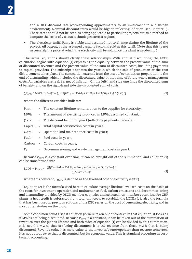
The actual equations should clarify these relationships. With annual discounting, the LCOE calculation begins with equation (1) expressing the equality between the present value of the sum of discounted revenues and the present value of the sum of discounted costs, including payments to capital providers. The subscript t denotes the year in which the sale of production or the cost disbursement takes place. The summation extends from the start of construction preparation to the end of dismantling, which includes the discounted value at that time of future waste management costs. All variables are real, i.e. net of inflation. On the left-hand side one finds the discounted sum of benefits and on the right-hand side the discounted sum of costs:

∑PMWh * MWh * (1+r)-t = ∑[(Capitalt + O&Mt + Fuelt + Carbont + Dt) * (1+r)-t] (1)

where the different variables indicate:

PMWh = The constant lifetime remuneration to the supplier for electricity;

MWh = The amount of electricity produced in MWh, assumed constant;

(1+r)-t = The discount factor for year t (reflecting payments to capital);

Capitalt = Total capital construction costs in year t;

O&Mt = Operation and maintenance costs in year t;

Fuelt = Fuel costs in year t;

Carbont = Carbon costs in year t;

Dt = Decommissioning and waste management costs in year t.

Because PMWh is a constant over time, it can be brought out of the summation, and equation (1) can be transformed into

LCOE = PMWh = ∑[(Capitalt + O&Mt + Fuelt + Carbont + Dt) * (1+r)-t] ∑ MWh (1+r)-t (2)

where this constant, PMWh, is defined as the levelised cost of electricity (LCOE).

Equation (2) is the formula used here to calculate average lifetime levelised costs on the basis of the costs for investment, operation and maintenance, fuel, carbon emissions and decommissioning and dismantling provided by OECD member countries and selected non-member countries. (For CHP plants, a heat credit is subtracted from total unit costs to establish the LCOE.) It is also the formula that has been used in previous editions of the EGC series on the cost of generating electricity, and in most other studies on the topic.

Some confusion could arise if equation (2) were taken out of context. In that equation, it looks as if MWhs are being discounted. Because PMWh is a constant, it can be taken out of the summation of revenues over the plant’s lifetime and both sides of equation (1) can be divided by this summation. It is not the MWhs that are being discounted; it is the revenue from those MWh that is being discounted. Revenue today has more value to the investor/owner/operator than revenue tomorrow. It is not output per se that is discounted, but its economic value. This is standard procedure in cost-benefit accounting.

29

2

29

Calculating the costs of generating electricity

Before presenting the different methodological conventions and default assumptions employed to harmonise the data received from different countries, one major underlying principle must be discussed: this report on Projected Costs of Generating Electricity is concerned with the levelised cost of producing baseload electricity at the plant level. While this seems straightforward, it has implications that are frequently less evident.

First, this implies that the assumptions on capacity factors are based on years of observation and were chosen to compare baseload technologies. For example, nuclear power plants can operate more than 90% capacity factors in years without refuelling outages, and combined-cycle natural gas turbines (CCGTs) can operate at less than 80% when they are too expensive to compete in the baseload market. For nuclear, coal and combined-cycle natural gas plants, a standard capacity factor of 85% was chosen by consensus. This is higher than the average observed capacity factors in practice, and particularly so for CCGT plants (this report does not consider steam cycle natural gas plants). The reason is that operators may choose to shut them down during baseload periods, when prices are low, owing to their higher marginal costs (for example owing to high natural gas prices). However, such considerations of portfolio optimisation do not enter into the methodology of this report.

Second, plant level costs imply that this report does not take into account system costs, i.e. the impact of a power plant on the electricity system as a whole. This is an issue that concerns all technologies, for instance in terms of location or grid connection. The issue of system costs, however, is a major issue for variable renewable energies, such as wind and solar. Because electricity cannot be stored, demand and supply must be balanced every second. (In the medium term, responsive demand enabled by “smart metering” and “smart grids”, and progress in electricity storage technologies could contribute to increase system flexibility and facilitate the integration of variable renewables.)

The variability of electricity from wind turbines or solar panels puts further strains on the ability to balance the system. While improvements in meteorology can help, they do not solve the problem. Even shortfalls announced in advance must be compensated by other sources of generation or demand response that can be mobilised on short notice, namely hydro reserves or natural gas peaking plants, which otherwise stay idle. Our discussion focuses only on technical system costs. Pecuniary system costs, however, can be considerable. At specific moments, prices for baseload electricity in Europe have been very low or negative for short periods thanks to overcapacity in the system, which is signalled by the market price. This issue is discussed in Chapters 10 and 11.

There is little disagreement among experts that such system costs for variable renewables exist, particularly at high levels of penetration. There is, however, little agreement (or little information) about their precise amount, which varies with the structure and interconnection of the energy system and the share of non-dispatchable renewables. Chapter 10, “The system cost and system value of electricity generation”, provides an overview of the available research on the topic, but without offering any conclusive estimates.

Finally, as has already been mentioned in the Introduction, this report considers social resource costs: the cost of society to build and operate a given plant, independent of all taxes, subsidies and transfers. The latter, for example in form of a tax credit or a faster amortisation schedule, can have a major impact on the profitability of a given project, particularly for distributed technologies where households are the investors paying value-added taxes. Hence, they affect the competitiveness of specific technologies, aside from their social resource cost.

Keeping in mind these caveats concerning the nature of the analysis, it is now possible to provide an overview of the more detailed methodological procedures employed to calculate the levelised cost of electricity (LCOE) for different technologies in different countries. This requires treading a fine line between capturing the specifics of each individual case on the one hand, and harmonising data to render them comparable, on the other.

30

2

30

2.2 Methodological conventions and key assumptions

The purpose of these methodological conventions for calculating levelised average lifetime costs with the EGC spreadsheet model is to guarantee comparability of the data received while preserving the country-specific information. Defining them in a satisfactory manner implies finding a careful balance between too much and too little homogenisation. These conventions have two distinct functions:

1. Assumptions on specific key parameters, such as discount rates, lifetimes, or fuel and carbon prices, need harmonisation because they have a decisive impact on final results. Different fuel price assumptions inside a single region – for example Europe – would bury all other information but reveal little about national conditions for electricity generation costs. Differences among regions or in some large countries, however, are acknowledged.

2. In the light of occasionally incomplete or ambiguous country submissions, methodological conventions serve to complete and harmonise these ambiguities (this concerns items such as contingency assumptions, residual value, decommissioning costs and schedules, and so on). Wherever possible, national assumptions were taken in these cases.

Decisions on methodology were prepared by the IEA and NEA Secretariats and taken by EGC Expert Group consensus. What follows is an overview of conventions and key assumptions.

Lifetimes

The following expected lifetimes were used as the default value for each technology, except in the cases where national data was provided:

Wind and solar plants: 25 years

Natural gas-fired CCGTs: 30 years

Coal-fired power and geothermal plants: 40 years

Nuclear power plants: 60 years

Hydropower: 80 years

Discount rates

The levelised costs of electricity were calculated for all technologies for 3%, 7% and 10% discount rates. (The discount factor is equal to the inverse of one plus the discount rate: 1/[1 + r].)

Capacity

Wherever the distinction was made in national submissions, net rather than gross capacity was used for calculations. This EGC report compares plants that have very different sizes, e.g. the costs of fossil fuel plants versus the cost of other technologies, which normally have significantly larger size units, such as nuclear power plants. The EGC methodology does not however take into account the economies of larger multiple-unit plants. It is estimated that new units built at an existing site may be 10% to 15% cheaper than greenfield units if they can use (at least partially) existing buildings, auxiliary facilities and infrastructure. Regulatory approvals are likely to be more straightforward. The number of units commissioned at the plant site also leads to a non-linear reduction of per-unit capital costs. If a two-unit plant is taken as a basis for comparison, the costs of the first unit may be nearly 20% to 25% higher because of the common costs for structures and equipment shared with the next unit.

31

2

31

Capacity factors

A standard capacity factor of 85% was used for all CCGTs, coal-fired and nuclear plants under the assumption that they operate in baseload. While it is clearly understood that many CCGTs are frequently used in mid-load or even peak load rather than in baseload, since the overarching concern here is with baseload capacity, the 85% assumption is also used as a generic assumption for CCGTs. However, in the sensitivity analyses, a 50% capacity factor is used to show the impact of this change on the LCOE. Country-specific capacity factors were used for renewable energies, because they are largely site-specific.

Overnight costs

Overnight construction costs include: i) direct construction costs plus pre-construction costs, such as site licensing, including the environmental testing; ii) the indirect costs such as engineering and administrative costs that cannot be associated with a specific direct construction cost category, as well as capitalised indirect costs; iii)  owners’ costs include expenses incurred by the owner(s) associated with the plant and plant site, but excluding off-site, “beyond the busbar”, transmission costs; and iv) contingency to account for changes in overnight cost during construction, for example 15%.

Contingency payments

Contingencies, increased costs resulting from unforeseen technical or regulatory events, are included in the last year of construction. The following conventions have been adopted if national data were not available:

Nuclear energy: 15% of overnight costs

All other technologies: 5% of overnight costs

Construction cost profiles

Allocation of costs during construction followed country indications. It is linear in cases where no precise indications were provided. In the absence of national indications for the length of construction periods, the following default consensus assumptions are used:

Non-hydro renewables: 1 year

Natural gas-fired power plants: 2 years

Coal-fired power plants: 4 years

Nuclear power plants: 7 years

Investment costs

Investment costs include overnight cost with contingency and financing costs (e.g. interest during construction), referred to in Equations (1) and (2) as total capital construction costs, or “capitalt”. On the other hand, “capital costs” in Chapter 4 include refurbishment and decommissioning costs.

Treatment of fixed operations and maintenance costs

Fixed O&M costs were added to each year in the cash flow model.

32

2

32

Fuel prices

Average OECD import price assumptions for hard (black) coal and natural gas were provided by the IEA Office of the Chief Economist and are comparable with the assumptions used in the World Energy Outlook (IEA, 2014). The average calorific values associated to these prices are based on the IEA energy statistics and balances of OECD countries. For the heat content of brown coal, national assumptions were used wherever available, which was the case for the great majority of countries. [In the absence of national mass-to-heat conversion factors, this report uses a default factor for hard coal of 25 gigajoules (GJ) per tonne.] The prices used are provided in standard commercial units for coal (tonnes) and for natural gas in million British thermal units (MMBtu).

Hard coal (OECD member countries): USD 101/tonne

Brown coal (not traded): National assumptions for both price and heat content

Natural gas (OECD Europe): USD 11.1/MMBtu

Natural gas (OECD Asia): USD 14.4/MMBtu

Natural gas (United States): USD 5.5/MMBtu

In the case of New Zealand (which produces the natural gas consumed by its gas-fired generation domestically), this report has adopted national assumptions for prices and heat content as provided by New Zealand government-nominated experts.

The major story in the world of natural gas remains the “shale gas revolution” and more broadly the development of unconventional gas in Canada and the United States. While it is possible that shale gas development will expand beyond North America at some point, it is unlikely to become a significant factor in other regions over the time frame of this report. Moreover, within the United States, at least some of the continued shift away from investment in coal-fired generation will be the result of increased environmental regulations, as opposed to relatively low gas prices. The degree to which increasing supply – including expanded liquefied natural gas (LNG) exports – and demand globally will impact natural gas prices over the medium term is also quite uncertain.

During the second half of 2014, however, fuel prices saw significant declines globally. The values assumed for this report were fixed before much of these declines, and therefore may be high relative to expectations at the time of publication. Of course, any view of fuel prices in 2020 will have significant underlying uncertainties. For a discussion on the impact of changes in fuel prices on the LCOE calculation, see Chapter 7. These fuel prices correspond to forecasts for 2020, date of the commercial operation of the plants (not over their lifetime), using the same methodology which was considered in the EGC 2010 report:

New Zealand

Natural gas: USD 5.8/MMBtu

National fuel price assumptions were also used for the non-OECD countries:

China

Hard coal: USD 112/tonne

Natural gas: USD 11.5/MMBtu

South Africa

Hard coal: USD 46.6/tonne

33

2

33

Costs of the “once-through” nuclear fuel cycle

Many countries provided cost data on different components of the fuel cycle, including the costs of recycling used fuel. However, to work with the EGC spreadsheet model, cost data in terms of USD/MWh needed to be defined on a harmonised basis. For uranium prices, an indicative value that does not directly enter the calculation of the front end of the nuclear fuel cycle is USD 100/kg of U3O8, which has been the average price during the last half century.

Front end of nuclear fuel cycle: USD 7/MWh (mining, enrichment, conditioning)

Back end of nuclear fuel cycle: USD 2.33/MWh (spent fuel removal, disposal and storage)

Wherever available in a compatible format, the EGC spreadsheet model uses national data.

Carbon price

The EGC model works with a harmonised carbon price common to all countries over the lifetime of all technologies. Many countries do not have an explicit carbon price. In these cases, USD 30 can be taken to be the shadow price of carbon, and not a cost that would be borne by investors.

All countries: USD 30/tonne of CO2

The carbon dioxide (CO2) module calculates the carbon cost per MWh. Whenever available, national data on carbon emissions per MWh are used. Otherwise, data were derived from IPCC (2006, Chapter 2 “Stationary Combustion”, p. 2.16).

Decommissioning and residual values

At the end of a plant’s lifetime, decommissioning costs and waste management costs are spread over a period of ten years for all technologies. In case of any positive “residual value” after the operating lifetime of a plant (iron scrap value, left-over carbon permits, etc.), there was a possibility to also report it. For fossil fuel plants, the residual value of equipment and materials shall normally be assumed to be equal to the cost of dismantling and site restoration, resulting in a zero net cost of decommissioning. For wind turbines and solar panels, rather than decommissioning, what takes place in practice at the end of their operating lifetime is a replacement of equipment, and the scrap value of the renewable installation is estimated to amount to 20% of the original capital investment. However, no country reported such residual values. In any case, wherever available, the submitted national values were used. Where no data on decommissioning costs were submitted, the following default values were used:

Nuclear energy: 15% of overnight costs

All other technologies: 5% of overnight costs

The question of decommissioning had led to discussions in the EGC Expert Group given that, because of the levelised cost methodology, decommissioning costs become small when discounted over 60 years (unless a lower discount rate is used, i.e. one more appropriate for trust fund management), the lifetime of a nuclear plant is assumed. In actual practice, the owner-operator makes annual contributions to a sinking fund (e.g. a financially segregated “decommissioning trust fund”) during operations for the eventual decommissioning and dismantlement (D&D, including waste management costs). It is the annual contributions for D&D and waste management that are included in the LCOE as a fixed operation and maintenance (O&M) cost. This fund usually earns a rate of return over the plant’s lifetime (assumed here to be 60 years), and hence is growing until D&D is completed (see NEA, 2003). Because of the long lifetime and the return on the fund, the annual contribution is thus a small part of a nuclear power plant’s LCOE (see PNNL, 2011).

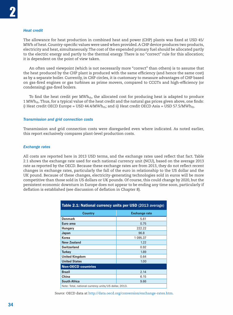
34

2

34

Heat credit

The allowance for heat production in combined heat and power (CHP) plants was fixed at USD 45/MWh of heat. Country-specific values were used when provided. A CHP device produces two products, electricity and heat, simultaneously. The cost of the expended primary fuel should be allocated partly to the electric energy and partly to the thermal energy. There is no “correct” rule for this allocation; it is dependent on the point of view taken.

An often used viewpoint (which is not necessarily more “correct” than others) is to assume that the heat produced by the CHP plant is produced with the same efficiency (and hence the same cost) as by a separate boiler. Currently, in CHP circles, it is customary to measure advantages of CHP based on gas-fired engines or gas turbines as prime movers, compared to CCGTs and high-efficiency (or condensing) gas-fired boilers.

To find the heat credit per MWhth, the allocated cost for producing heat is adapted to produce 1 MWhth. Thus, for a typical value of the heat credit and the natural gas prices given above, one finds: i) Heat credit OECD Europe = USD 44.4/MWhth; and ii) Heat credit OECD Asia = USD 57.5/MWhth.

Transmission and grid connection costs

Transmission and grid connection costs were disregarded even where indicated. As noted earlier, this report exclusively compares plant-level production costs.

Exchange rates

All costs are reported here in 2013 USD terms, and the exchange rates used reflect that fact. Table 2.1 shows the exchange rate used for each national currency unit (NCU), based on the average 2013 rate as reported by the OECD. Because these exchange rates are from 2013, they do not reflect recent changes in exchange rates, particularly the fall of the euro in relationship to the US dollar and the UK pound. Because of these changes, electricity-generating technologies sold in euros will be more competitive than those sold in US dollars or UK pounds. Of course, this could change by 2020, but the persistent economic downturn in Europe does not appear to be ending any time soon, particularly if deflation is established (see discussion of deflation in Chapter 8).

Table 2.1: National currency units per USD (2013 average)

Country Exchange rate

Denmark 5.61Euro area 0.75Hungary 222.22Japan 96.8Korea 1 095.37New Zealand 1.22Switzerland 0.92Turkey 1.89United Kingdom 0.64United States 1.00

Non-OECD countries

Brazil 2.14China 6.15South Africa 9.66Note: Total, national currency units/US dollar, 2013.

Source: OECD data at http://data.oecd.org/conversion/exchange-rates.htm.

35

2

35

2.3 Conclusions

This overview described the conventions and key assumptions adopted for calculating the levelised cost of electricity generation. While individual assumptions can be subject to discussion – and several of them have been the subject of vigorous debate in the EGC Expert Group – one should not lose sight of their essential function, which is to render comparable large amounts of heterogeneous data. In fact, only by rendering the data comparable can the specificity of each individual dataset be brought out and assessed.

The key assumptions and methodological conventions presented above should thus not be mistaken for an “IEA or NEA Secretariat view” or an “EGC Expert Group view”. All those involved are sufficiently informed to know that the future cost of power generation is uncertain. Even more so, these assumptions should not be mistaken for an official OECD view on the costs of electricity generation. As a whole, the above key assumptions and conventions serve to develop reasonable base cases that can be starting points for better inquiries.

Readers thus must develop their own views. They are assisted in this task by the many sensitivity analyses in Part II that show the impact of varying some key assumptions. This report intends to encourage further work and discussion on the costs of power generation rather than to be a substitute for such more detailed work.

References

IEA (2014), World Energy Outlook, OECD, Paris, www.worldenergyoutlook.org/.

IEA/NEA (2010), Projected Costs of Generating Electricity, 2010 Edition, OECD, Paris, www.iea.org/publications/freepublications/publication/projected_costs.pdf

IPPC (2006), IPCC Guidelines for National Greenhouse Gas Inventories, Intergovernmental Panel on Climate Change, World Meteorological Organization, Geneva, www.ipcc-nggip.iges.or.jp/public/2006gl/.

NEA (2003), Decommissioning Nuclear Power Plants: Policies, Strategies and Costs, OECD, Paris (this report is an update of the 2010 edition), www.oecd-ilibrary.org/nuclear-energy/decommissioning-nuclear- power-plants_9789264104334-en.

PNNL (2011), Assessment of the Adequacy of the 10 CFR 50.75(c) Minimum Decommissioning Fund Formula, Office of Nuclear Material Reactor Regulation, Pacific Northwest National Laboratory for the US Nuclear Regulatory Commission, Richland, WA, http://pbadupws.nrc.gov/docs/ML1306/ML13063A190.pdf.

37

3

37

Chapter

Technology overview This chapter presents an overview of the technologies included in this report. Section 3.1 includes a summary of overnight and investment costs, capacities, and other relevant technical specifications for all 181 plants in the EGC 2015 database.1 Section 3.2 provides the plant-by-plant LCOE calculations, including a breakdown of the LCOE cost components, for each plant in the report, separated according to their technology category.

All cost figures are given in 2013 US dollars. The assumed commissioning date is 2020, unless noted otherwise.

3.1 Overview of different generating technologies

The EGC 2015 dataset includes a wide range of generating technologies, including natural gas-fired generation (both combined-cycle gas turbines, or CCGTs, and open-cycle gas turbines, or OCGTs), coal-fired generation, various types of nuclear generation, solar photovoltaic (of varying sizes) and concentrated solar power (CSP), onshore and offshore wind, geothermal, biomass, and combined heat and power (based on a large variety of fuel types).

Table 3.1 presents size and overnight cost statistics for the various technologies included here. The paragraphs and tables that follow describe in more detail the characteristics of the generating technologies, as well as some of the non-cost specifications for the corresponding plants.

Table 3.1: Summary statistics for different generating technologies

Technology Number of plants

Net capacity1 (MWe) Overnight cost2 (USD/kWe)

Min Mean Median Max Min Mean Median Max

Natural gas – CCGT 13 350 551 475 900 627 1 021 1 014 1 289Natural gas – OCGT 4 50 274 240 565 500 708 699 933Coal 14 605 1 131 772 4 693 813 2 080 2 264 3 067Nuclear 11 535 1 434 1 300 3 300 1 807 4 249 4 896 6 215Solar PV – residential 12 0.003 0.007 0.005 0.02 1 867 2 379 2 297 3 366Solar PV – commercial 14 0.05 0.34 0.22 1.0 728 1 583 1 696 1 977Solar PV – large 12 1 19.3 2.5 200 937 1 555 1 436 2 563Solar thermal (CSP) 4 50 135 146 200 3 571 5 964 6 072 8 142Onshore wind 21 2 38 20 200 1 200 1 911 1 804 2 999Offshore wind 12 2 275 223 833 3 703 4 985 4 998 5 933Hydro – small 12 0.4 3.1 2 10 1 369 5 127 5 281 9 400Hydro – large 16 11 1 093 50 13 050 598 3 492 2 493 8 687Geothermal 6 6.8 62 27 250 1 493 4 898 5 823 6 625Biomass and biogas 11 0.2 154 10 900 587 4 447 4 060 8 667CHP (all types) 19 0.2 5.3 1.1 62 926 4 526 2 926 15 9881. Net capacity may refer to the unit capacity or to the combined capacity of multiple units on the same site.2. Overnight cost includes pre-construction (owner’s), construction (engineering, procurement and construction) and contingency costs, but not

interest during construction (IDC).

1. For additional details on the underlying data and their various sources, please contact the study authors.

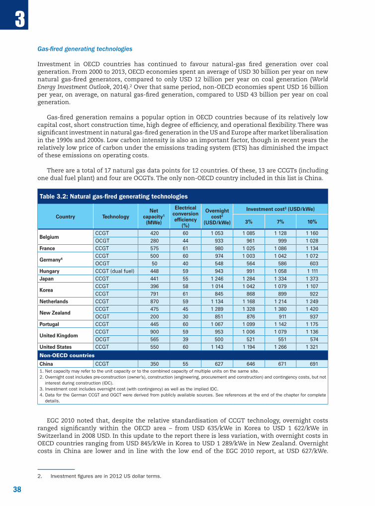
38

3

38

Gas-fired generating technologies

Investment in OECD countries has continued to favour natural-gas fired generation over coal generation. From 2000 to 2013, OECD economies spent an average of USD 30 billion per year on new natural gas-fired generators, compared to only USD 12 billion per year on coal generation (World Energy Investment Outlook, 2014).2 Over that same period, non-OECD economies spent USD 16 billion per year, on average, on natural gas-fired generation, compared to USD 43 billion per year on coal generation.

Gas-fired generation remains a popular option in OECD countries because of its relatively low capital cost, short construction time, high degree of efficiency, and operational flexibility. There was significant investment in natural gas-fired generation in the US and Europe after market liberalisation in the 1990s and 2000s. Low carbon intensity is also an important factor, though in recent years the relatively low price of carbon under the emissions trading system (ETS) has diminished the impact of these emissions on operating costs.

There are a total of 17 natural gas data points for 12 countries. Of these, 13 are CCGTs (including one dual fuel plant) and four are OCGTs. The only non-OECD country included in this list is China.

Table 3.2: Natural gas-fired generating technologies

Country TechnologyNet

capacity1 (MWe)

Electrical conversion efficiency

(%)

Overnight cost2

(USD/kWe)

Investment cost3 (USD/kWe)

3% 7% 10%

BelgiumCCGT 420 60 1 053 1 085 1 128 1 160OCGT 280 44 933 961 999 1 028

France CCGT 575 61 980 1 025 1 086 1 134

Germany4CCGT 500 60 974 1 003 1 042 1 072OCGT 50 40 548 564 586 603

Hungary CCGT (dual fuel) 448 59 943 991 1 058 1 111Japan CCGT 441 55 1 246 1 284 1 334 1 373

KoreaCCGT 396 58 1 014 1 042 1 079 1 107CCGT 791 61 845 868 899 922

Netherlands CCGT 870 59 1 134 1 168 1 214 1 249

New ZealandCCGT 475 45 1 289 1 328 1 380 1 420OCGT 200 30 851 876 911 937

Portugal CCGT 445 60 1 067 1 099 1 142 1 175

United KingdomCCGT 900 59 953 1 006 1 079 1 136OCGT 565 39 500 521 551 574

United States CCGT 550 60 1 143 1 194 1 266 1 321

Non-OECD countries

China CCGT 350 55 627 646 671 6911. Net capacity may refer to the unit capacity or to the combined capacity of multiple units on the same site.2. Overnight cost includes pre-construction (owner’s), construction (engineering, procurement and construction) and contingency costs, but not

interest during construction (IDC).3. Investment cost includes overnight cost (with contingency) as well as the implied IDC.4. Data for the German CCGT and OGCT were derived from publicly available sources. See references at the end of the chapter for complete

details.

EGC 2010 noted that, despite the relative standardisation of CCGT technology, overnight costs ranged significantly within the OECD area – from USD 635/kWe in Korea to USD 1  622/kWe in Switzerland in 2008 USD. In this update to the report there is less variation, with overnight costs in OECD countries ranging from USD 845/kWe in Korea to USD 1 289/kWe in New Zealand. Overnight costs in China are lower and in line with the low end of the EGC 2010 report, at USD 627/kWe.

2. Investment figures are in 2012 US dollar terms.

39

3

39

Despite the relative standardisation of CCGT technologies, it is reasonable to expect overnight costs for CCGTs to diverge, even in the case where technologies are deployed in countries that seem relatively similar. This is because the actual cost of construction depends on a number of factors that go beyond the technology itself, including technical issues such as different operating requirements, and regulatory issues such as different grid codes, safety standards or labour costs.

As noted in Chapter 2, all CCGTs have been modelled with a default capacity factor of 85%. In addition, a 50% capacity factor sensitivity was modelled, as detailed in Section 3.3.

Coal-fired generating technologies

The EGC 2015 dataset contains only 14 coal plants, compared to 48 in EGC 2010 (14 of which included carbon capture and storage, a technology that was excluded from this update). As noted earlier, within OECD countries there has been a marked shift away from coal generation towards natural gas-fired generation. With regard to non-OECD countries, this updated report includes only one coal plant from China, versus three in EGC 2010, and none from Brazil, which contributed one data point to the previous report. In addition, the Russian Federation did not participate in the EGC 2015 report, but did contribute two coal plants to the 2010 report.

Table 3.3: Coal-fired generating technologies

Country TechnologyNet

capacity1 (MWe)

Electrical conversion efficiency

(%)

Overnight cost2

(USD/kWe)

Investment cost3 (USD/kWe)

3% 7% 10%

Belgium Ultra-supercritical 750 46 2 307 2 448 2 648 2 807

Germany4Hard coal 700 46 1 643 1 744 1 887 1 999Lignite 900 43 2 054 2 180 2 358 2 499

Japan Ultra-supercritical 704 41 2 496 2 649 2 866 3 037

KoreaPulverised (PC 1000) 960 43 1 218 1 289 1 386 1 463Pulverised (PC 800) 766 41 1 252 1 317 1 407 1 477

NetherlandsUltra-supercritical 1 070 46 1 620 1 720 1 860 1 971Ultra-supercritical 777 46 2 746 2 914 3 152 3 341Ultra-supercritical 1 554 46 2 660 2 823 3 054 3 237

PortugalPulverised 605 51 3 067 3 255 3 521 3 732Pulverised 605 46 2 533 2 689 2 909 3 083

United States Supercritical pulverised 750 43 2 496 2 609 2 765 2 886

Non-OECD countries

China Ultra-supercritical 1 000 45 813 863 933 989South Africa Pulverised 4 693 40 2 222 2 588 3 157 3 6521. Net capacity may refer to the unit capacity or to the combined capacity of multiple units on the same site.2. Overnight cost includes pre-construction (owner’s), construction (engineering, procurement and construction) and contingency costs, but

not IDC.3. Investment cost includes overnight cost (with contingency) as well as the implied IDC.4. Data for the German coal plants were derived from publicly available sources. See references at the end of the chapter for complete details.

The plants in the EGC 2015 database operate at efficiency levels ranging from 41% (Japan and Korea) and 51% (Portugal), as measured on the fuel’s lower heating value basis (net calorific value) and range in size from 605 MW (Portugal) to 4 693 MW (a multi-unit plant in South Africa). Among OECD countries, the largest coal plant is in the Netherlands (1  554  MW). Overnight costs among OECD countries range from USD 1 218/kWe in Korea to USD 3 067/kWe in Portugal. In non-OECD countries, overnight costs are USD 2 222/kWe in South Africa, and USD 813/kWe in China.

As with CCGTs, and nuclear below, all coal plants have been modelled at a default capacity factor of 85%. In addition, a 50% capacity factor sensitivity is detailed in Section 3.3.

40

3

40

The EGC 2015 database contains only supercritical and ultra-supercritical plants. Both supercritical and ultra-supercritical plants operate above the water-steam critical point, which requires pressures in excess of 221 bars (by comparison, a subcritical plant will generally operate at a pressure of around 165 bars). Above the water-steam critical point, water will change from liquid to steam without boiling – that is, there is no observed change in state and there is no latent heat requirement. Supercritical designs are employed in order to improve the overall efficiency of the generator. There is no standard definition for ultra-supercritical versus supercritical, though in general any plant that operates above 600oC is considered to be ultra-supercritical. Typical supercritical and ultra-supercritical plants use steam at pressures from 240 bar to 300 bar and temperatures up to 620oC.3

Supercritical plants are more expensive to build than subcritical plants because, while they may be simpler in design (requiring no steam drum to separate steam and water), they require more expensive materials, more complex boilers, and more precise control systems. The increase in cost is usually justified by the efficiency gains.

Nuclear generating technologies

The EGC 2015 database contains 11 nuclear power plants, of which 9 are in OECD member countries (the remaining two are in China). This includes a generic light water reactor (LWR), ten advanced light water reactors and generic generation III reactors.4 For new designs, net plant capacities range from around 1 000 to 3 300 MW (for a multiple-unit plant in the United Kingdom). Nuclear technologies are very capital-intensive, and differing regulatory requirements, technical capacities and financial conditions lead to a wide range of overnight costs in OECD countries – from USD 2 021/kWe in Korea to USD 6 215/kWe in Hungary. The range of investment costs is large as it includes various reactor designs, as well as country-specific project constraints (e.g. working rules, safety requirements, regulation) and economic conditions (e.g. labour costs).

As in EGC 2010, all the reactors in this report are based on light water technologies, indicating that the industry trend towards this technology continues. LWRs can either be pressurised water (PWR) or boiling water (BWR). In PWRs, water is kept under high pressure so that it remains in liquid state, while BWRs, as the name implies, allow the water to boil. In both reactor types, heat is drawn away from the reactor core to create steam and drive turbine generators. Both reactor types have advanced versions, designated generically as ALWRs.

In keeping with the EGC 2010 general assumption for open fuel cycle, front-end fuel cycle costs are USD 7/MWh, versus USD 2.33/MWh for back-end fuel cycle. (There are too few data to determine the cost of a closed fuel cycle until a strategy for managing used mixed plutonium-uranium fuel is available.) Country-specific costs were used when provided. Front-end fuel cycle costs include uranium mining and milling, conversion, enrichment and fuel fabrication. Back-end fuel cycle costs, which are counted from the point after the spent fuel is unloaded from the reactor, may refer to one of two options: direct disposal (or once-through cycle) or recycling (reprocessing fuel cycle). In the once-through cycle, spent fuel is allowed to cool and then conditioned for long-term storage. Under reprocessing, the recyclable portion of the spent fuel (approximately 95% of the mass) is separated from the fission products and minor actinides. Separated plutonium and uranium may then be reused as a component of mixed oxide (MOX) fuel in light water reactors or stored for a future utilisation in fast spectrum reactors. The reprocessed high-level waste (HLW) is stored, usually in vitrified form. The total (front- and back-end) cost is relatively independent of the fuel cycle process itself, as processes that have higher upfront costs tend to have correspondingly lower back-end costs, and vice-versa.5

3. Potential future developments for coal technologies are discussed in Chapter 9.

4. The nuclear power plant in Mohovce, Slovak Republic, is the completion of a project originally initiated in 1986, the design of which has evolved substantially from the original water-cooled and water-moderated energy reactor (VVER) V-213 specifications. The expert group decided to keep this project as part of this section since the completion is expected in the time frame of interest for our study, but some caution is needed when taking into account the specificity of that project.

5. For more on this topic, see Economics of the Back End of the Nuclear Fuel Cycle, www.oecd-nea.org/ndd/pubs/2013/7061-ebenfc.pdf.

41

3

41

Table 3.4: Nuclear generating technologies

Country TechnologyNet

capacity1 (MWe)

Overnight cost2

(USD/kWe)

Investment cost3 (USD/kWe)

3% 7% 10%

Belgium Gen III projects 1 000-1 600 5 081 5 645 6 498 7 222Finland ALWR 1 600 4 896 5 439 6 261 6 959France ALWR 1 630 5 067 5 629 6 479 7 202Hungary ALWR 1 180 6 215 6 756 7 535 8 164Japan ALWR 1 152 3 883 4 313 4 965 5 519Korea ALWR 1 343 2 021 2 177 2 400 2 580Slovak Republic LWR 2 x 535 4 986 5 573 6 472 7 243United Kingdom ALWR 3 300 6 070 6 608 7 399 8 053United States ALWR 1 400 4 100 4 555 5 243 5 828

Non-OECD countries

ChinaALWR 1 250 2 615 2 905 3 344 3 717ALWR 1 080 1 807 2 007 2 310 2 568

1. Net capacity may refer to the unit capacity or to the combined capacity of multiple units on the same site.2. Overnight cost includes pre-construction (owner’s), construction (engineering, procurement and construction) and contingency

costs, but not IDC.3. Investment cost includes overnight cost (with contingency) as well as the implied IDC.

Note: The cost for Belgium is based on a generic, nth-of-a-kind generation III nuclear plant. Cost figures for France are estimations for a series of plants commissioned at 2030 horizon, as opposed to 2020 for other plants in the database. The overnight cost figure corresponds to an average of a range which could be between USD 4 530 and 5 600/kW. The Hungarian overnight cost data have been calculated from a nominal CAPEX of EUR 12.5 billion (for two VVER-1200 reactors) and an assumed inflation rate of 2%. The Slovak plant is the completion of a project originally initiated in 1986, with a substantially updated design.

All nuclear reactors in the report were modelled using a standard average annual capacity factor of 85%. The capacity factor is a measure of the amount of electricity produced over a year, compared to the maximum amount of electricity that could be produced if the plant operated continuously. In 2013, the reported average capacity factors for nuclear power plants in OECD countries was 82.4% (IAEA PRIS),6 slightly lower than the reported capacity factor for 2008, which was used as a reference point in EGC 2010. Thus, 85% remains the default assumption.7 In keeping with the modelling of natural gas and coal plants, nuclear generators are also modelled at a 50% capacity factor. Given current nuclear plant designs, however, it is extremely unlikely that a nuclear reactor would be built under those operating conditions.

Decommissioning costs for nuclear plants are higher than those for other generation types, in part because of the additional cost of removing all remaining radioactive materials. Plant-specific decommissioning costs were used when provided, and a default assumption of 15% of the overnight cost was used for all other plants (compared to a default of 5% for other generators). Because of the relatively high overnight cost of nuclear plants, decommissioning costs are also relatively high, at least in nominal terms. However, decommissioning costs are a relatively small component of a nuclear plant’s LCOE, mainly because of the impact of discounting. The default assumption for a nuclear plant’s lifetime is 60 years. Decommissioning costs, as modelled in this report, are only incurred at the end of the plant’s life, and so in net present value terms they are close to zero even under a low discount rate of 3%.

6. IAEA PRIS is a database available online at the IAEA website: www.iaea.org/pris/. This capacity factor is based on a survey of reactors in OECD countries. Nuclear power plants in Japan have not been considered in this analysis.

7. In some cases, higher capacity factors have been provided by a few countries.

42

3

42

Renewable energy technologies

The EGC 2015 database suggests a clear shift of focus towards renewable energy. In total, 138 renewable plants are included, compared to 72 in EGC 2010. This includes 38 solar PV plants of varying sizes and 4 solar thermal plants (of which 3 have some form of storage), 21 onshore wind and 12 offshore wind installations, 6 biomass and biogas plants, 27 hydro plants, 11 geothermal installations, and 19 CHP plants (based on both renewable and non-renewable energy sources).

Solar PV: The cost of solar PV installations can roughly be divided into two components: the modules, and balance of system (BOS) items such as the support structure, inverters, and the cost of installation. While the modules themselves have become fairly standardised products, as the EGC 2015 data show, there is still significant variation in total solar PV costs globally. Different supply chains, local regulatory requirements, labour and permitting costs, and different financing mechanisms can all lead to widely different final costs, even if the cost of the components is relatively similar.8

It is also worth noting that, though solar PV plants have a relatively short construction time,9 the overnight cost component of the LCOE still depends heavily on the discount rate. This is because LCOE calculation discounts future MWh generation. As a result, generation at the end of the solar PV installation’s lifetime is of relatively less value than generation closer to the time of construction.

In this updated report, solar PV plants are divided into three categories: residential rooftop (less than 20 kWe), commercial rooftop (from 20 kWe to 1 MWe), and large, ground-mounted (greater than 1 MW). Capacities range from .003 MWe to 200 MWe, and capacity factors range from 10% to 21% (in the United States). Overnight costs for residential PV range from USD 1 867/kWe in Portugal to USD 3 366/kWe in France (which includes additional costs specific to building-integrated solar systems); commercial PV overnight costs range from USD 1 029/kWe in Austria to USD 1 967/kWe in Korea; and for large, ground-mounted PV, costs range from USD 1 200/kWe in Germany to USD 2 563/kWe in Japan.

Solar thermal (CSP): Several solar thermal installations have been built over the past few years, in particular in regions such as Spain and the south-western United States, where there is significant sunlight and large amounts of space. Solar thermal technologies are able to produce significant amounts of power (installation sizes tend to range from the tens to hundreds of megawatts) and can be used with thermal storage solutions such as molten salts to extend their electric power production into peak evening hours. Conversely, solar thermal power plants use more materials – in particular steel – than other types of solar power, and so are relatively more capital-intensive and will often also have higher operation and maintenance (O&M) costs.

While the absolute number of expected solar thermal, or concentrated solar power (CSP), installations in the database is relatively low, in capacity terms, solar thermal represents a significant portion of total solar power dataset. Of the 679 MW of solar power in the database (PV included), 450 MW are solar thermal. Of this, 300 MW of solar thermal generation include some form of storage. Overnight costs range from USD 3 571/kWe in the United States to USD 8 142/kWe in Spain and depend largely on the sizes of solar fields and storage relative to the rated capacity.

Table 3.5: Solar generating technologies

Country TechnologyNet

capacity (MWe)

Capacity factor

(%)

Annual efficiency loss (%)

Overnight cost1

(USD/kWe)

Investment cost2 (USD/kWe)

3% 7% 10%

Austria Solar PV – commercial rooftop 0.2 11 0.5 1 029 1 045 1 065 1 079

BelgiumSolar PV – residential rooftop 0.0-0.02 11 0.5 2 303 2 338 2 383 2 416Solar PV – commercial rooftop 0.02-1.0 11 0.5 1 653 1 678 1 710 1 734

DenmarkSolar PV – residential rooftop 0.01 12 0.4 2 310 2 344 2 389 2 422Solar PV – commercial rooftop 0.1 13 0.4 1 977 2 007 2 045 2 074Solar PV – large, ground-mounted 4.0 14 0.4 1 885 1 913 1 950 1 977

FranceSolar PV – residential rooftop3 0.003 14 0.5 3 366 3 416 3 482 3 530Solar PV – commercial rooftop 0.3 14 0.5 1 800 1 827 1 862 1 888Solar PV – large, ground-mounted 2 15 0.5 1 400 1 421 1 448 1 468

8. For more on this, see the IEA’s Medium Term Renewable Energy Market Report 2014, OECD/IEA, Paris.

9. The average construction time for solar PV plants in the EGC study is one year.

8. For more on this, see the IEA’s Medium Term Renewable Energy Market Report 2014, OECD/IEA, Paris.

9. The average construction time for solar PV plants in the EGC study is one year.

43

3

43

Table 3.5 (cont’d)

Country TechnologyNet

capacity (MW)

Capacity factor

(%)

Annual efficiency loss (%)

Overnight cost1

(USD/kWe)

Investment cost2 (USD/kWe)

3% 7% 10%

GermanySolar PV – residential rooftop 0.01 11 0.4 2 000 2 030 2 069 2 098Solar PV – commercial rooftop 0.5 11 0.4 1 467 1 489 1 517 1 538Solar PV – large, ground-mounted 5 11 0.4 1 200 1 218 1 241 1 259

HungarySolar PV – residential rooftop 0.003 13 0.5 2 100 2 134 2 178 2 210Solar PV – commercial rooftop 0.05 13 0.5 1 890 1 918 1 955 1 983Solar PV – large, ground-mounted 1 13 0.5 1 890 1 919 1 958 1 986

ItalySolar PV – residential rooftop 0.003 15 0.7 2 315 2 349 2 394 2 428Solar PV – commercial rooftop 0.09 15 0.7 1 763 1 789 1 824 1 849Solar PV – large, ground-mounted 1.7 15 0.7 1 363 1 384 1 410 1 430

JapanSolar PV – residential rooftop 0.004 12 0.5 3 101 3 147 3 207 3 252Solar PV – large, ground-mounted 2 14 0.5 2 563 2 601 2 651 2 688

KoreaSolar PV – residential rooftop 0.01 13 0.5 2 404 2 440 2 487 2 521Solar PV – commercial rooftop 0.1 14 0.5 1 967 1 996 2 035 2 063Solar PV – large, ground-mounted 3 15 0.5 1 794 1 821 1 856 1 882

Netherlands Solar PV – commercial rooftop 0.1 11 0.5 1 257 1 278 1 305 1 325

PortugalSolar PV – residential rooftop 0.01 17 0.5 1 867 1 894 1 931 1 958Solar PV – commercial rooftop 0.5 17 0.5 1 333 1 353 1 379 1 398Solar PV – large, ground-mounted 1 18 0.5 1 467 1 489 1 517 1 538

Spain

Solar PV – residential rooftop 0.02 19 0.5 1 939 1 972 2 016 2 048Solar PV – commercial rooftop 0.1 19 0.5 1 599 1 627 1 663 1 690Solar PV – large, ground-mounted 5.0 19 0.5 1 238 1 261 1 291 1 314Solar thermal (CSP) – no storage 50 31 0.0 8 142 8 297 8 502 8 655

Switzerland Solar PV – commercial rooftop 1 14 0.3 1 957 1 989 2 032 2 063

United KingdomSolar PV – residential rooftop 0.003 10 0.5 2 500 2 537 2 586 2 622Solar PV – large, ground-mounted 5 11 0.5 1 406 1 427 1 455 1 475

United States

Solar PV – residential rooftop 0.0-0.02 15 0.5 2 250 2 284 2 327 2 360Solar PV – commercial rooftop 0.02-1.0 15 0.5 1 739 1 765 1 799 1 824Solar PV – large, ground-mounted 20 21 0.5 1 603 1 627 1 658 1 681Solar thermal (CSP) – 6 hrs storage 200 34 0.0 3 571 3 624 3 694 3 745Solar thermal (CSP) – 12 hrs storage 200 55 0.0 4 901 4 974 5 070 5 140

Non-OECD countries

ChinaSolar PV – commercial rooftop 0.5 12 0.5 728 739 754 764Solar PV – large, ground-mounted 200 17 0.5 937 951 970 983

South Africa Solar thermal (CSP) – molten salt storage 92 60 0.0 7 243 7 866 8 762 9 488

1. Overnight cost includes pre-construction (owner’s), construction (engineering, procurement and construction) and contingency costs, but not IDC.2. Investment cost includes overnight cost (with contingency) as well as the implied IDC.3. Costs in France, for residential rooftop, include additional costs specific to roof-integrated solar systems.

Onshore wind: Onshore wind has, by most measures, become a mature and fairly standard product. Overnight costs for OECD countries range from USD  1  571/kWe in the United States to USD  2  999/kWe in Japan. Cost in non-OECD countries range from USD  1  200/kWe in China to USD 2 757/kWe in South Africa. Capacity factors across all countries range from 20% to 49%. The EGC 2010 noted that, under an assumed learning rate of 7%, overnight costs for onshore wind could reach as low as USD 1 400/kWe by 2020. The only county in the EGC 2015 dataset with plant costs that are low is China, but within OECD countries there are notable declines relative to the 2010 report, where costs ranged from USD 1 821/kWe to USD 3 716/kWe.

Offshore wind: Offshore wind has become a relatively mature technology in northern Europe but experiences elsewhere have been fairly limited. The EGC 2015 database contains 12 data points for offshore wind plants, compared to 7 in EGC 2010 – a modest but notable increase. Overnight costs range from USD 3 703/kWe in the United Kingdom to USD 5 846/kWe in the United States. Capacity factors range from 30% to 48%. Here, costs remain relatively in line with EGC 2010, which had offshore wind plants ranging from USD 2 540/kWe to USD 5 554/kWe.

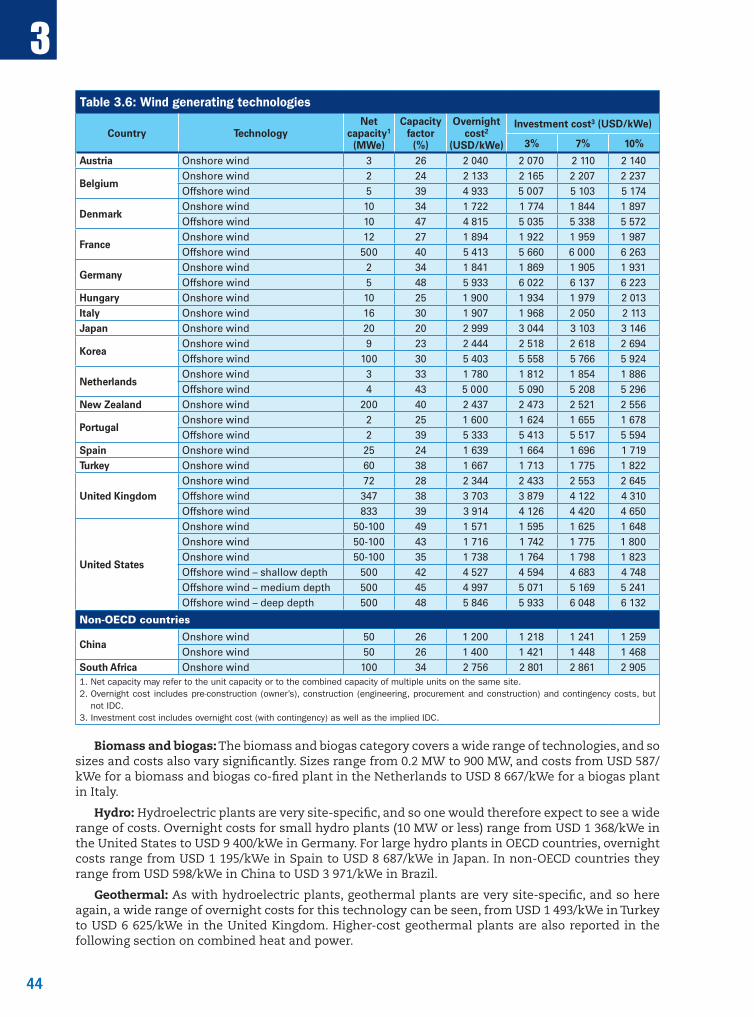
44

3

44

Table 3.6: Wind generating technologies

Country TechnologyNet

capacity1 (MWe)

Capacity factor

(%)

Overnight cost2

(USD/kWe)

Investment cost3 (USD/kWe)

3% 7% 10%

Austria Onshore wind 3 26 2 040 2 070 2 110 2 140

BelgiumOnshore wind 2 24 2 133 2 165 2 207 2 237Offshore wind 5 39 4 933 5 007 5 103 5 174

DenmarkOnshore wind 10 34 1 722 1 774 1 844 1 897Offshore wind 10 47 4 815 5 035 5 338 5 572

FranceOnshore wind 12 27 1 894 1 922 1 959 1 987Offshore wind 500 40 5 413 5 660 6 000 6 263

GermanyOnshore wind 2 34 1 841 1 869 1 905 1 931Offshore wind 5 48 5 933 6 022 6 137 6 223

Hungary Onshore wind 10 25 1 900 1 934 1 979 2 013Italy Onshore wind 16 30 1 907 1 968 2 050 2 113Japan Onshore wind 20 20 2 999 3 044 3 103 3 146

KoreaOnshore wind 9 23 2 444 2 518 2 618 2 694Offshore wind 100 30 5 403 5 558 5 766 5 924

NetherlandsOnshore wind 3 33 1 780 1 812 1 854 1 886Offshore wind 4 43 5 000 5 090 5 208 5 296

New Zealand Onshore wind 200 40 2 437 2 473 2 521 2 556

PortugalOnshore wind 2 25 1 600 1 624 1 655 1 678Offshore wind 2 39 5 333 5 413 5 517 5 594

Spain Onshore wind 25 24 1 639 1 664 1 696 1 719Turkey Onshore wind 60 38 1 667 1 713 1 775 1 822

United KingdomOnshore wind 72 28 2 344 2 433 2 553 2 645Offshore wind 347 38 3 703 3 879 4 122 4 310Offshore wind 833 39 3 914 4 126 4 420 4 650

United States

Onshore wind 50-100 49 1 571 1 595 1 625 1 648Onshore wind 50-100 43 1 716 1 742 1 775 1 800Onshore wind 50-100 35 1 738 1 764 1 798 1 823Offshore wind – shallow depth 500 42 4 527 4 594 4 683 4 748Offshore wind – medium depth 500 45 4 997 5 071 5 169 5 241Offshore wind – deep depth 500 48 5 846 5 933 6 048 6 132

Non-OECD countries

ChinaOnshore wind 50 26 1 200 1 218 1 241 1 259Onshore wind 50 26 1 400 1 421 1 448 1 468

South Africa Onshore wind 100 34 2 756 2 801 2 861 2 9051. Net capacity may refer to the unit capacity or to the combined capacity of multiple units on the same site.2. Overnight cost includes pre-construction (owner’s), construction (engineering, procurement and construction) and contingency costs, but

not IDC.3. Investment cost includes overnight cost (with contingency) as well as the implied IDC.

Biomass and biogas: The biomass and biogas category covers a wide range of technologies, and so sizes and costs also vary significantly. Sizes range from 0.2 MW to 900 MW, and costs from USD 587/kWe for a biomass and biogas co-fired plant in the Netherlands to USD 8 667/kWe for a biogas plant in Italy.

Hydro: Hydroelectric plants are very site-specific, and so one would therefore expect to see a wide range of costs. Overnight costs for small hydro plants (10 MW or less) range from USD 1 368/kWe in the United States to USD 9 400/kWe in Germany. For large hydro plants in OECD countries, overnight costs range from USD 1 195/kWe in Spain to USD 8 687/kWe in Japan. In non-OECD countries they range from USD 598/kWe in China to USD 3 971/kWe in Brazil.

Geothermal: As with hydroelectric plants, geothermal plants are very site-specific, and so here again, a wide range of overnight costs for this technology can be seen, from USD 1 493/kWe in Turkey to USD 6 625/kWe in the United Kingdom. Higher-cost geothermal plants are also reported in the following section on combined heat and power.

45

3

45

Table 3.7: Other renewable generating technologies

Country Technology Net capacity1 (MWe)

Capacity factor

(%)

Overnight cost2

(USD/kWe)

Investment cost3 (USD/kWe)

3% 7% 10%

Austria Small hydro – run-of-river 2.2 51 2 977 3 308 3 807 4 232

GermanySmall hydro – run-of-river 2 55 9 400 10 448 12 028 13 367Large hydro – run-of-river 20 63 6 600 7 347 8 473 9 427

Italy

Small hydro – run-of-river 0.4 49 5 929 6 138 6 421 6 638Biogas – engine 0.3 80 8 667 8 934 9 294 9 567Solid biomass – turbine 0.2 86 6 945 7 170 7 474 7 705Solid waste incineration 10 84 5 800 5 975 6 210 6 387Geothermal 20 92 5 653 5 824 6 053 6 226

Japan Large hydro 12 45 8 687 9 651 11 109 12 348

NetherlandsCo-firing of wood pellets 640 80 587 607 635 656Solid waste incineration 20 85 3 427 3 538 3 688 3 802

New Zealand Geothermal 250 89 3 331 3 431 3 566 3 668

PortugalLarge hydro – reservoir 144 17 2 933 3 259 3 751 4 170Large hydro – pumped storage 218 28 3 733 4 147 4 774 5 307

Spain

Small hydro – reservoir 2 40 1 661 1 711 1 779 1 830Small hydro – run-of-river 2 39 2 588 2 706 2 869 2 995Large hydro – reservoir 20 40 1 195 1 231 1 279 1 316Large hydro – run-of-river 20 39 1 859 1 943 2 060 2 151Biogas – engine 1 48 1 852 1 880 1 916 1 942Biogas – engine 1.5 48 3 733 3 789 3 862 3 916Biomass – turbine 10 75 4 060 4 245 4 501 4 698Solid waste incineration – turbine 15 56 8 540 8 930 9 467 9 882

Switzerland

Small hydro – run-of-river 10 54 6 848 7 607 8 757 9 734Large hydro – pumped storage 1 000 26 1 630 1 811 2 085 2 318Large hydro – reservoir 50 28 6 890 7 655 8 811 9 794Large hydro – run-of-river 50 50 6 185 6 871 7 909 8 791

TurkeyGeothermal 24 90 1 493 1 587 1 719 1 824Large hydro – reservoir 19 54 2 052 2 146 2 277 2 379

United Kingdom

Large hydro 11 35 5 234 5 427 5 688 5 886Biomass 900 65 719 732 750 764Geothermal 6.8 91 6 625 7 046 7 635 8 096

United States

Hydro – non-power dams 0.1 to multi MW 65 1 369 1 521 1 751 1 946Hydro – non-power dams 0.1 to multi MW 62 5 039 5 598 6 443 7 162Hydro – non-power dams 0.1 to multi MW 58 9 099 10 109 11 637 12 935Hydro – new stream development 0.1 to multi MW 68 3 568 3 963 4 562 5 071Hydro – new stream development 0.1 to multi MW 66 5 524 6 136 7 064 7 852Hydro – new stream development 0.1 to multi MW 62 7 522 8 357 9 619 10 692Biomass 100 85 4 587 4 794 5 081 5 303Geothermal – binary rankine cycle 30 80 6 291 6 480 6 735 6 928Geothermal – flash steam 40 90 5 992 6 172 6 415 6 599

Non-OECD countries

Brazil

Large hydro 270 56 1 589 1 693 1 841 1 959Large hydro – run-of-river 800 55 1 567 1 665 1 804 1 914Large hydro – run-of-river 15 57 3 971 4 175 4 459 4 680Large hydro – run-of-river 1 800 52 1 151 1 252 1 399 1 519

China Large hydro – reservoir 13 050 52 598 664 764 8501. Net capacity may refer to the unit capacity or to the combined capacity of multiple units on the same site.2. Overnight cost includes pre-construction (owner’s), construction (engineering, procurement and construction) and contingency costs, but

not IDC.3. Investment cost includes overnight cost (with contingency) as well as the implied IDC.

Note: The Netherlands’ co-firing generator refers to a plant with 20% biomass and 80% coal; costs indicated only cover the cost of biomass compared to an (existing) coal power plant. Non-power dams in the United States are dams that have been converted from non-power producing to power producing.

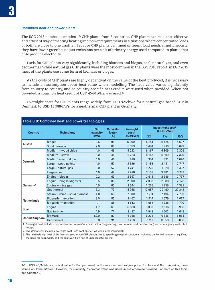
46

3

46

Combined heat and power plants

The EGC 2015 database contains 19 CHP plants from 6 countries. CHP plants can be a cost-effective and efficient way of meeting heating and power requirements in situations where concentrated loads of both are close to one another. Because CHP plants can meet different load needs simultaneously, they have lower greenhouse gas emissions per unit of primary energy used compared to plants that only produce electricity.

Fuels for CHP plants vary significantly, including biomass and biogas, coal, natural gas, and even geothermal. While natural gas CHP plants were the most common in the EGC 2010 report, in EGC 2015 most of the plants use some form of biomass or biogas.

As the costs of CHP plants are highly dependent on the value of the heat produced, it is necessary to include an assumption about heat value when modelling. The heat value varies significantly from country to country, and so country-specific heat credits were used when provided. When not provided, a common heat credit of USD 45/MWhth was used.10

Overnight costs for CHP plants range widely, from USD 926/kWe for a natural gas-based CHP in Denmark to USD 15 988/kWe for a geothermal CHP plant in Germany.

Table 3.8: Combined heat and power technologies

Country TechnologyNet

capacity (MWe)

Capacity factor

(%)

Overnight cost1

(USD/kWe)

Investment cost2 (USD/kWe)

3% 7% 10%

AustriaBiogas 0.5 91 6 000 6 181 6 424 6 607Solid biomass 2.0 80 5 333 5 494 5 710 5 873

Denmark

Medium – wood chips 1.0 46 5 723 6 167 6 809 7 329Medium – straw 1.0 46 5 723 6 167 6 809 7 329Medium – natural gas 1.0 46 926 954 991 1 020Large – wood pellets 1.0 57 2 926 3 153 3 481 3 747Large – natural gas 1.0 57 1 241 1 278 1 328 1 367Large – coal 1.0 49 2 926 3 153 3 481 3 747

Germany3

Engine – biogas 0.2 63 2 567 2 618 2 686 2 737Engine – biogas (digester) 0.5 80 2 000 2 038 2 088 2 126Engine – mine gas 1.5 80 1 244 1 268 1 298 1 321Geothermal 3.3 73 15 988 17 657 20 190 22 348Steam turbine – solid biomass 4.0 68 7 000 7 211 7 494 7 709

NetherlandsBiogas/fermentation 3.0 85 1 467 1 514 1 579 1 627Biogas/fermentation 1.1 85 1 613 1 666 1 736 1 790

SpainEngine 4.7 63 8 638 9 033 9 576 9 996Gas turbine 4.9 71 1 497 1 542 1 602 1 648

United KingdomBiomass 62.0 83 5 938 6 235 6 645 6 964Geothermal 6.8 91 7 250 7 710 8 353 8 856

1. Overnight cost includes pre-construction (owner’s), construction (engineering, procurement and construction) and contingency costs, but not IDC.

2. Investment cost includes overnight cost (with contingency) as well as the implied IDC.3. The relatively high cost of the German geothermal CHP plant is due to specific geological conditions, including the limited number of aquifers,

the need for deep wells, and the relatively high risk of unsuccessful drilling.

10. USD 45/MWh is a typical value for Europe based on the assumed natural gas price. For Asia and North America, these values would be different. However, for simplicity, a common value was used unless otherwise provided. For more on this topic, see Chapter 2.

47

3

47

3.2 Technology-by-technology data on electricity generating costs

Tables 3.9 to 3.15 present the calculated LCOEs for each of the 181 power plants included in the EGC 2015 dataset, along with the relevant cost components, calculated at each of the three discount rates (3%, 7% and 10%). For each power plant, the net capacity, overnight cost, refurbishment and decommissioning costs, and O&M costs are presented. Construction, refurbishment and decommissioning costs for all plants are dependent on the discount rate used, and so the costs presented are calculated at each discount rate. Depending on the plant-specific O&M schedules, O&M costs may also vary depending on the discount rate, and in these cases the discount rate specific costs are presented. Also included are the fuel, waste and carbon costs, when relevant. For fossil plants a column indicating the electrical conversion efficiency is included. All cost figures are given in 2013 US dollars.

Before presenting the figures, it is worth emphasising that an explicit comparison of LCOEs for different technologies and even among countries can be misleading, as each technology and each country faces a different set of risk profiles. A more detailed discussion of this topic can be found in Chapter 8.

The LCOEs for natural gas, coal, and nuclear plants are all calculated at the same assumed capacity factor of 85%.11 Plant-specific capacity factors were used for all renewable power plants and CHP plants. These are presented in the relevant tables. For solar PV, for the first time an annual efficiency loss factor is included. When provided, country-specific factors were used. For all other plants, a default rate of 0.5% per annum was used.

For CHP plants, the calculated heat credit is also provided. The heat credit is subtracted from the LCOE, and so is presented in negative terms.12

11. Alternate LCOEs assuming a 50% capacity factor are presented in Section 3.3.

12. For CHP plants, consistent with the LCOE methodology, total CO2 emissions and their associated costs have been allocated entirely to the electricity output. While this does raise the cost of electricity, it also increases the total value of the heat credit. The deduction from gross electricity costs is therefore higher, and so allocating the carbon cost to electricity only or splitting it between electricity and heat production does not materially impact the final results.

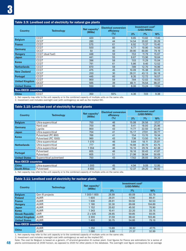
48

3

48

Table 3.9: Levelised cost of electricity for natural gas plants

Country Technology Net capacity1 (MWe)

Electrical conversion efficiency

(%)

Investment cost2 (USD/MWh)

Refurbishment and decom­missioning costs (USD/MWh) Fuel cost

(USD/MWh)Carbon cost (USD/MWh)

O&M costs (USD/MWh)

LCOE (USD/MWh) Country

3% 7% 10% 3% 7% 10% 3% 7% 10%

BelgiumCCGT 420 60 9.65 13.82 17.45 0.21 0.12 0.07 74.62 10.08 3.97 98.54 102.61 106.19

BelgiumOCGT 280 44 14.54 20.82 26.28 0.32 0.17 0.11 100.91 14.01 5.35 135.13 141.26 146.66

France CCGT 575 61 6.92 11.37 15.40 0.11 0.05 0.02 68.99 10.56 6.25 92.83 97.21 101.23 France

GermanyCCGT 500 60 6.77 10.90 14.56 0.11 0.05 0.02 74.00 9.90 7.71 98.49 102.56 106.20

GermanyOCGT 50 40 39.90 60.80 79.19 0.76 0.36 0.20 111.00 15.15 29.68 196.50 216.99 235.23

Hungary CCGT (dual fuel) 448 59 7.53 11.79 15.67 0.00 0.00 0.00 71.21 10.56 7.64 96.94 101.20 105.08 HungaryJapan CCGT 441 55 8.67 13.96 18.64 0.15 0.06 0.03 104.07 10.95 9.38 133.21 138.42 143.07 Japan

KoreaCCGT 396 58 7.03 11.29 15.04 0.00 0.00 0.00 98.97 10.27 5.55 121.82 126.08 129.82

KoreaCCGT 791 61 5.86 9.40 12.52 0.10 0.04 0.02 95.21 9.89 4.05 115.11 118.60 121.70

Netherlands CCGT 870 59 7.89 12.70 16.96 0.13 0.05 0.03 75.25 9.90 3.53 96.71 101.45 105.68 Netherlands

New ZealandCCGT 475 45 10.09 15.38 20.03 0.19 0.09 0.05 46.75 11.22 7.38 75.64 80.82 85.43

New ZealandOCGT 200 30 28.31 43.13 56.18 0.54 0.26 0.14 69.26 16.62 14.39 129.11 143.65 156.58

Portugal CCGT 445 60 8.35 12.72 16.57 0.16 0.08 0.04 74.00 9.90 6.24 98.65 102.93 106.75 Portugal

United KingdomCCGT 900 59 7.64 12.02 16.03 0.00 0.00 0.00 75.51 9.43 6.63 99.21 103.59 107.59

United KingdomOCGT 565 39 48.11 74.54 98.37 0.00 0.00 0.00 113.85 14.22 36.45 212.63 239.06 262.89

United States CCGT 550 60 8.06 13.24 17.94 0.13 0.05 0.03 36.90 11.10 4.65 60.84 65.95 70.62 United States

Non-OECD countries Non-OECD countriesChina CCGT 350 55% 4.36 7.03 9.38 0.07 0.03 0.01 71.47 11.02 3.25 90.17 92.79 95.13 China1. Net capacity may refer to the unit capacity or to the combined capacity of multiple units on the same site.2. Investment cost includes overnight cost (with contingency) as well as the implied IDC.

Note: CCGTs were modelled under an assumed capacity factor of 85%. OCGTs were modelled under nationally provided capacity factors.

Table 3.10: Levelised cost of electricity for coal plants

Country Technology Net capacity1 (MWe)

Electrical conversion efficiency

(%)

Investment cost2 (USD/MWh)

Refurbishment and decom­missioning costs (USD/MWh) Fuel cost

(USD/MWh)Carbon cost (USD/MWh)

O&M costs (USD/MWh)

LCOE (USD/MWh) Country

3% 7% 10% 3% 7% 10% 3% 7% 10%

Belgium Ultra-supercritical 750 46 15.08 26.56 37.27 0.21 0.07 0.03 26.67 22.05 8.00 72.00 83.35 94.02 Belgium

GermanyHard coal 700 46 9.41 18.00 25.96 0.10 0.03 0.01 26.38 21.98 9.14 67.01 75.53 83.47

GermanyLignite 900 43 11.77 22.50 32.45 0.12 0.03 0.01 14.88 28.20 11.07 66.04 76.69 86.61

Japan Ultra-supercritical 704 41 15.17 27.91 39.77 0.19 0.06 0.02 35.91 25.02 18.52 94.81 107.42 119.25 Japan

KoreaPulverised (PC 800) 766 41 7.54 13.70 19.34 0.00 0.00 0.00 40.04 24.77 5.31 77.66 83.83 89.46

KoreaPulverised (PC 1000) 960 43 7.38 13.50 19.16 0.09 0.03 0.01 38.36 23.67 4.80 74.30 80.36 86.00

NetherlandsUltra-supercritical 1 070 46 9.84 18.11 25.81 0.12 0.04 0.01 31.49 21.90 8.88 72.23 80.42 88.09

NetherlandsUltra-supercritical 777 46 16.68 30.70 43.75 0.20 0.06 0.02 31.49 21.90 8.88 79.15 93.03 106.04Ultra-supercritical 1 554 46 16.16 29.74 42.38 1.84 2.34 2.68 31.49 22.20 7.81 79.51 93.58 106.56

PortugalPulverised 605 46 18.16 30.43 41.87 0.29 0.12 0.06 31.47 22.21 6.16 78.28 90.39 101.77

PortugalPulverised 605 51 21.98 36.84 50.69 0.35 0.15 0.07 28.38 20.03 14.53 85.27 99.93 113.71

United States Supercritical pulverised 750 43 17.62 28.93 39.20 0.29 0.12 0.06 28.42 25.20 11.12 82.64 93.79 104.00 United States

Non-OECD countries Non-OECD countriesChina Ultra-supercritical 1 000 45 4.94 9.09 12.95 0.06 0.02 0.01 35.67 28.88 4.07 73.61 77.72 81.57 ChinaSouth Africa Pulverised 4 693 40 12.37 29.20 46.92 0.07 0.01 0.00 20.45 27.00 5.41 65.31 82.07 99.79 South Africa1. Net capacity may refer to the unit capacity or to the combined capacity of multiple units on the same site. 2. Investment cost includes overnight cost (with contingency) as well as the implied IDC.

Table 3.11: Levelised cost of electricity for nuclear plants

Country Technology Net capacity1 (MWe)

Investment cost2 (USD/MWh)

Refurbishment and decom­missioning costs (USD/MWh)

Fuel and waste costs (USD/MWh)

Carbon cost (USD/MWh)

O&M costs (USD/MWh)

LCOE (USD/MWh) Country

3% 7% 10% 3% 7% 10% 3% 7% 10%

Belgium Gen III projects 1 000-1 600 26.99 60.09 92.79 0.46 0.08 0.02 10.46 0.00 13.55 51.45 84.17 116.81 BelgiumFinland ALWR 1 600 26.01 57.90 89.41 0.44 0.06 0.01 5.09 0.00 14.59 46.13 77.64 109.10 FinlandFrance ALWR 1 630 26.91 59.92 92.53 0.40 0.06 0.01 9.33 0.00 13.33 49.98 82.64 115.21 FranceHungary ALWR 1 180 32.30 69.68 104.89 1.59 0.26 0.06 9.60 0.00 10.40 53.90 89.94 124.95 HungaryJapan ALWR 1 152 20.62 45.92 70.90 0.42 0.07 0.02 14.15 0.00 27.43 62.63 87.57 112.50 JapanKorea ALWR 1 343 10.41 22.20 33.15 0.00 0.00 0.00 8.58 0.00 9.65 28.63 40.42 51.37 KoreaSlovak Republic LWR 2 x 535 26.65 59.85 93.05 4.65 1.50 0.83 12.43 0.00 10.17 53.90 83.95 116.48 Slovak RepublicUnited Kingdom ALWR 3 300 31.59 68.42 103.46 0.54 0.09 0.02 11.31 0.00 20.93 64.38 100.75 135.72 United KingdomUnited States ALWR 1 400 30.75 54.86 79.16 1.26 0.52 0.26 11.33 0.00 11.00 54.34 77.71 101.76 United States

Non-OECD countries Non-OECD countries

ChinaALWR 1 250 13.89 30.92 47.75 0.23 0.04 0.01 9.33 0.00 7.32 30.77 47.61 64.40

ChinaALWR 1 080 9.60 21.37 32.99 0.16 0.03 0.01 9.33 0.00 6.50 25.59 37.23 48.831. Net capacity may refer to the unit capacity or to the combined capacity of multiple units on the same site.2. Investment cost includes overnight cost (with contingency) as well as the implied IDC.Note: The cost for Belgium is based on a generic, nth-of-a-kind generation III nuclear plant. Cost figures for France are estimations for a series of plants commissioned at 2030 horizon, as opposed to 2020 for other plants in the database. The overnight cost figure corresponds to an average

of a range which could be between USD 4 530 and 5 600/kW. The Hungarian overnight cost data have been calculated from a nominal CAPEX of EUR 12.5 billion (for two VVER-1200 reactors) and an assumed inflation rate of 2%. The Slovak plant is the completion of a project originally initiated in 1986, with a substantially updated design.

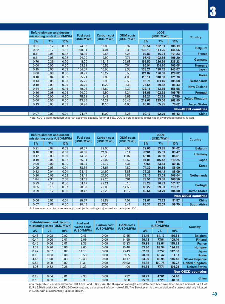
49

3

49

Table 3.9: Levelised cost of electricity for natural gas plants

Country Technology Net capacity1 (MWe)

Electrical conversion efficiency

(%)

Investment cost2 (USD/MWh)

Refurbishment and decom­missioning costs (USD/MWh) Fuel cost

(USD/MWh)Carbon cost (USD/MWh)

O&M costs (USD/MWh)

LCOE (USD/MWh) Country

3% 7% 10% 3% 7% 10% 3% 7% 10%

BelgiumCCGT 420 60 9.65 13.82 17.45 0.21 0.12 0.07 74.62 10.08 3.97 98.54 102.61 106.19

BelgiumOCGT 280 44 14.54 20.82 26.28 0.32 0.17 0.11 100.91 14.01 5.35 135.13 141.26 146.66

France CCGT 575 61 6.92 11.37 15.40 0.11 0.05 0.02 68.99 10.56 6.25 92.83 97.21 101.23 France

GermanyCCGT 500 60 6.77 10.90 14.56 0.11 0.05 0.02 74.00 9.90 7.71 98.49 102.56 106.20

GermanyOCGT 50 40 39.90 60.80 79.19 0.76 0.36 0.20 111.00 15.15 29.68 196.50 216.99 235.23

Hungary CCGT (dual fuel) 448 59 7.53 11.79 15.67 0.00 0.00 0.00 71.21 10.56 7.64 96.94 101.20 105.08 HungaryJapan CCGT 441 55 8.67 13.96 18.64 0.15 0.06 0.03 104.07 10.95 9.38 133.21 138.42 143.07 Japan

KoreaCCGT 396 58 7.03 11.29 15.04 0.00 0.00 0.00 98.97 10.27 5.55 121.82 126.08 129.82

KoreaCCGT 791 61 5.86 9.40 12.52 0.10 0.04 0.02 95.21 9.89 4.05 115.11 118.60 121.70

Netherlands CCGT 870 59 7.89 12.70 16.96 0.13 0.05 0.03 75.25 9.90 3.53 96.71 101.45 105.68 Netherlands

New ZealandCCGT 475 45 10.09 15.38 20.03 0.19 0.09 0.05 46.75 11.22 7.38 75.64 80.82 85.43

New ZealandOCGT 200 30 28.31 43.13 56.18 0.54 0.26 0.14 69.26 16.62 14.39 129.11 143.65 156.58

Portugal CCGT 445 60 8.35 12.72 16.57 0.16 0.08 0.04 74.00 9.90 6.24 98.65 102.93 106.75 Portugal

United KingdomCCGT 900 59 7.64 12.02 16.03 0.00 0.00 0.00 75.51 9.43 6.63 99.21 103.59 107.59

United KingdomOCGT 565 39 48.11 74.54 98.37 0.00 0.00 0.00 113.85 14.22 36.45 212.63 239.06 262.89

United States CCGT 550 60 8.06 13.24 17.94 0.13 0.05 0.03 36.90 11.10 4.65 60.84 65.95 70.62 United States

Non-OECD countries Non-OECD countriesChina CCGT 350 55% 4.36 7.03 9.38 0.07 0.03 0.01 71.47 11.02 3.25 90.17 92.79 95.13 China1. Net capacity may refer to the unit capacity or to the combined capacity of multiple units on the same site.2. Investment cost includes overnight cost (with contingency) as well as the implied IDC.

Note: CCGTs were modelled under an assumed capacity factor of 85%. OCGTs were modelled under nationally provided capacity factors.

Table 3.10: Levelised cost of electricity for coal plants

Country Technology Net capacity1 (MWe)

Electrical conversion efficiency

(%)

Investment cost2 (USD/MWh)

Refurbishment and decom­missioning costs (USD/MWh) Fuel cost

(USD/MWh)Carbon cost (USD/MWh)

O&M costs (USD/MWh)

LCOE (USD/MWh) Country

3% 7% 10% 3% 7% 10% 3% 7% 10%

Belgium Ultra-supercritical 750 46 15.08 26.56 37.27 0.21 0.07 0.03 26.67 22.05 8.00 72.00 83.35 94.02 Belgium

GermanyHard coal 700 46 9.41 18.00 25.96 0.10 0.03 0.01 26.38 21.98 9.14 67.01 75.53 83.47

GermanyLignite 900 43 11.77 22.50 32.45 0.12 0.03 0.01 14.88 28.20 11.07 66.04 76.69 86.61

Japan Ultra-supercritical 704 41 15.17 27.91 39.77 0.19 0.06 0.02 35.91 25.02 18.52 94.81 107.42 119.25 Japan

KoreaPulverised (PC 800) 766 41 7.54 13.70 19.34 0.00 0.00 0.00 40.04 24.77 5.31 77.66 83.83 89.46

KoreaPulverised (PC 1000) 960 43 7.38 13.50 19.16 0.09 0.03 0.01 38.36 23.67 4.80 74.30 80.36 86.00

NetherlandsUltra-supercritical 1 070 46 9.84 18.11 25.81 0.12 0.04 0.01 31.49 21.90 8.88 72.23 80.42 88.09

NetherlandsUltra-supercritical 777 46 16.68 30.70 43.75 0.20 0.06 0.02 31.49 21.90 8.88 79.15 93.03 106.04Ultra-supercritical 1 554 46 16.16 29.74 42.38 1.84 2.34 2.68 31.49 22.20 7.81 79.51 93.58 106.56

PortugalPulverised 605 46 18.16 30.43 41.87 0.29 0.12 0.06 31.47 22.21 6.16 78.28 90.39 101.77

PortugalPulverised 605 51 21.98 36.84 50.69 0.35 0.15 0.07 28.38 20.03 14.53 85.27 99.93 113.71

United States Supercritical pulverised 750 43 17.62 28.93 39.20 0.29 0.12 0.06 28.42 25.20 11.12 82.64 93.79 104.00 United States

Non-OECD countries Non-OECD countriesChina Ultra-supercritical 1 000 45 4.94 9.09 12.95 0.06 0.02 0.01 35.67 28.88 4.07 73.61 77.72 81.57 ChinaSouth Africa Pulverised 4 693 40 12.37 29.20 46.92 0.07 0.01 0.00 20.45 27.00 5.41 65.31 82.07 99.79 South Africa1. Net capacity may refer to the unit capacity or to the combined capacity of multiple units on the same site. 2. Investment cost includes overnight cost (with contingency) as well as the implied IDC.

Table 3.11: Levelised cost of electricity for nuclear plants

Country Technology Net capacity1 (MWe)

Investment cost2 (USD/MWh)

Refurbishment and decom­missioning costs (USD/MWh)

Fuel and waste costs (USD/MWh)

Carbon cost (USD/MWh)

O&M costs (USD/MWh)

LCOE (USD/MWh) Country

3% 7% 10% 3% 7% 10% 3% 7% 10%

Belgium Gen III projects 1 000-1 600 26.99 60.09 92.79 0.46 0.08 0.02 10.46 0.00 13.55 51.45 84.17 116.81 BelgiumFinland ALWR 1 600 26.01 57.90 89.41 0.44 0.06 0.01 5.09 0.00 14.59 46.13 77.64 109.10 FinlandFrance ALWR 1 630 26.91 59.92 92.53 0.40 0.06 0.01 9.33 0.00 13.33 49.98 82.64 115.21 FranceHungary ALWR 1 180 32.30 69.68 104.89 1.59 0.26 0.06 9.60 0.00 10.40 53.90 89.94 124.95 HungaryJapan ALWR 1 152 20.62 45.92 70.90 0.42 0.07 0.02 14.15 0.00 27.43 62.63 87.57 112.50 JapanKorea ALWR 1 343 10.41 22.20 33.15 0.00 0.00 0.00 8.58 0.00 9.65 28.63 40.42 51.37 KoreaSlovak Republic LWR 2 x 535 26.65 59.85 93.05 4.65 1.50 0.83 12.43 0.00 10.17 53.90 83.95 116.48 Slovak RepublicUnited Kingdom ALWR 3 300 31.59 68.42 103.46 0.54 0.09 0.02 11.31 0.00 20.93 64.38 100.75 135.72 United KingdomUnited States ALWR 1 400 30.75 54.86 79.16 1.26 0.52 0.26 11.33 0.00 11.00 54.34 77.71 101.76 United States

Non-OECD countries Non-OECD countries

ChinaALWR 1 250 13.89 30.92 47.75 0.23 0.04 0.01 9.33 0.00 7.32 30.77 47.61 64.40

ChinaALWR 1 080 9.60 21.37 32.99 0.16 0.03 0.01 9.33 0.00 6.50 25.59 37.23 48.831. Net capacity may refer to the unit capacity or to the combined capacity of multiple units on the same site.2. Investment cost includes overnight cost (with contingency) as well as the implied IDC.Note: The cost for Belgium is based on a generic, nth-of-a-kind generation III nuclear plant. Cost figures for France are estimations for a series of plants commissioned at 2030 horizon, as opposed to 2020 for other plants in the database. The overnight cost figure corresponds to an average

of a range which could be between USD 4 530 and 5 600/kW. The Hungarian overnight cost data have been calculated from a nominal CAPEX of EUR 12.5 billion (for two VVER-1200 reactors) and an assumed inflation rate of 2%. The Slovak plant is the completion of a project originally initiated in 1986, with a substantially updated design.

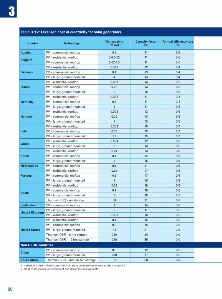
50

3

50

Table 3.12: Levelised cost of electricity for solar generators

Country Technology Net capacity (MWe)

Capacity factor (%)

Annual efficiency loss (%)

Investment cost1 (USD/MWh)

O&M costs2 (USD/MWh)

LCOE (USD/MWh) Country

3% 7% 10% 3% 7% 10% 3% 7% 10%

Austria PV – commercial rooftop 0.2 11 0.5 62.34 92.30 117.81 6.36 5.68 5.40 68.70 97.97 123.20 Austria

BelgiumPV – residential rooftop 0.0-0.02 11 0.5 167.62 233.98 289.98 22.00 21.87 21.78 189.62 255.85 311.77

BelgiumPV – commercial rooftop 0.02-1.0 11 0.5 120.29 167.91 208.11 22.00 21.87 21.78 142.29 189.78 229.89

Denmark

PV – residential rooftop 0.006 12 0.4 107.80 176.63 235.40 3.79 2.76 2.43 111.58 179.39 237.84

DenmarkPV – commercial rooftop 0.1 13 0.4 85.17 139.57 186.00 2.99 2.17 1.92 88.16 141.74 187.92

PV – large, ground-mounted 4 14 0.4 75.40 123.54 164.65 2.65 1.93 1.70 78.04 125.47 166.35

France

PV – residential rooftop 0.003 14 0.5 169.65 251.19 320.61 44.24 42.13 41.21 213.89 293.32 361.82

FrancePV – commercial rooftop 0.25 14 0.5 90.73 134.34 171.46 42.72 41.41 40.81 133.44 175.75 212.27

PV – large, ground-mounted 2 15 0.5 65.14 96.45 123.10 39.07 38.06 37.58 104.21 134.50 160.68

Germany

PV – residential rooftop 0.005 11 0.4 128.10 190.01 242.81 33.46 33.21 33.06 161.56 223.23 275.87

GermanyPV – commercial rooftop 0.5 11 0.4 92.47 137.16 175.27 24.15 23.98 23.86 116.62 161.13 199.13

PV – large, ground-mounted 5 11 0.4 72.96 108.23 138.30 19.06 18.92 18.83 92.02 127.14 157.13

Hungary

PV – residential rooftop 0.003 13 0.5 134.62 188.19 233.48 29.51 21.60 16.87 164.13 209.78 250.35

HungaryPV – commercial rooftop 0.05 13 0.5 121.04 168.97 209.44 13.72 10.06 7.87 134.76 179.04 217.31

PV – large, ground-mounted 1 13 0.5 121.10 169.17 209.78 44.33 40.90 38.80 165.43 210.07 248.57

Italy

PV – residential rooftop 0.003 15 0.7 109.59 161.76 206.06 49.39 47.69 46.88 158.98 209.45 252.94

ItalyPV – commercial rooftop 0.09 15 0.7 83.46 123.20 156.94 57.68 56.14 55.37 141.14 179.34 212.31

PV – large, ground-mounted 1.7 15 0.7 64.55 95.28 121.37 49.62 48.36 47.73 114.17 143.65 169.11

JapanPV – residential rooftop 0.004 12 0.5 178.41 264.16 337.16 39.70 37.44 36.48 218.11 301.60 373.65

JapanPV – large, ground-mounted 2 14 0.5 126.41 187.17 238.90 54.09 52.26 51.43 180.51 239.43 290.33

Korea

PV – residential rooftop 0.01 13 0.5 127.69 189.06 241.31 27.86 27.61 27.45 155.56 216.67 268.76

KoreaPV – commercial rooftop 0.1 14 0.5 100.61 148.96 190.13 21.95 21.75 21.63 122.56 170.71 211.75

PV – large, ground-mounted 3 15 0.5 84.00 124.38 158.75 17.86 17.70 17.59 101.86 142.07 176.34

Netherlands PV – commercial rooftop 0.1 11 0.5 76.27 113.15 144.64 24.75 23.72 23.27 101.02 136.87 167.90 Netherlands

Portugal

PV – residential rooftop 0.01 17 0.5 75.82 112.26 143.28 20.33 19.38 18.97 96.14 131.64 162.25

PortugalPV – commercial rooftop 0.5 17 0.5 54.16 80.18 102.34 19.91 19.18 18.86 74.06 99.37 121.20

PV – large, ground-mounted 1 18 0.5 56.26 83.30 106.32 18.90 18.16 17.83 75.16 101.46 124.16

Spain

PV – residential rooftop 0.02 19 0.5 63.93 99.99 130.90 36.67 36.03 35.80 100.60 136.02 166.70

SpainPV – commercial rooftop 0.1 19 0.5 52.73 82.49 107.98 50.23 49.53 49.23 102.97 132.01 157.21

PV – large, ground-mounted 5 19 0.5 40.89 64.07 83.98 46.43 45.85 45.59 87.33 109.92 129.57

Thermal (CSP) – no storage 50 31 0.0 172.60 259.30 334.25 90.79 89.04 88.35 263.39 348.35 422.60

Switzerland PV – commercial rooftop 1 14 0.3 84.57 132.86 174.36 30.74 29.73 29.34 115.32 162.59 203.70 Switzerland

United KingdomPV – large, ground-mounted 5 11 0.5 88.27 130.70 166.82 37.40 37.06 36.85 125.67 167.76 203.66

United KingdomPV – residential rooftop 0.003 10 0.5 142.33 232.30 308.88 44.92 44.18 43.75 187.25 276.47 352.63

United States

PV – residential rooftop 0.1 15 0.5 91.62 142.88 186.63 14.30 13.23 12.82 105.92 156.12 199.45

United States

PV – commercial rooftop 0.8 15 0.5 70.82 110.45 144.27 7.57 6.79 6.50 78.39 117.24 150.76

PV – large, ground-mounted 1.5 21 0.5 48.01 74.87 97.79 5.50 4.96 4.76 53.50 79.84 102.56

Thermal (CSP) – 6 hrs storage 250 34 0.0 60.58 95.68 125.95 17.97 17.38 17.17 78.54 113.06 143.12

Thermal (CSP) – 12 hrs storage 250 55 0.0 51.59 81.48 107.26 14.38 13.88 13.70 65.97 95.36 120.96

Non-OECD countries Non-OECD countries

ChinaPV – commercial rooftop 0.5 12 0.5 41.92 62.06 79.21 17.07 16.64 16.47 58.99 78.70 95.69

ChinaPV – large, ground-mounted 200 17 0.5 37.85 56.04 71.53 16.99 16.61 16.45 54.84 72.64 87.98

South Africa Thermal (CSP) – molten salt storage 92 60 0.0 84.68 138.30 189.62 54.59 53.78 53.47 139.27 192.08 243.09 South Africa

1. Investment cost includes overnight cost (with contingency) as well as the implied IDC.2. O&M costs include refurbishment and decommissioning costs.

51

3

51

Table 3.12: Levelised cost of electricity for solar generators

Country Technology Net capacity (MWe)

Capacity factor (%)

Annual efficiency loss (%)

Investment cost1 (USD/MWh)

O&M costs2 (USD/MWh)

LCOE (USD/MWh) Country

3% 7% 10% 3% 7% 10% 3% 7% 10%

Austria PV – commercial rooftop 0.2 11 0.5 62.34 92.30 117.81 6.36 5.68 5.40 68.70 97.97 123.20 Austria

BelgiumPV – residential rooftop 0.0-0.02 11 0.5 167.62 233.98 289.98 22.00 21.87 21.78 189.62 255.85 311.77

BelgiumPV – commercial rooftop 0.02-1.0 11 0.5 120.29 167.91 208.11 22.00 21.87 21.78 142.29 189.78 229.89

Denmark

PV – residential rooftop 0.006 12 0.4 107.80 176.63 235.40 3.79 2.76 2.43 111.58 179.39 237.84

DenmarkPV – commercial rooftop 0.1 13 0.4 85.17 139.57 186.00 2.99 2.17 1.92 88.16 141.74 187.92

PV – large, ground-mounted 4 14 0.4 75.40 123.54 164.65 2.65 1.93 1.70 78.04 125.47 166.35

France

PV – residential rooftop 0.003 14 0.5 169.65 251.19 320.61 44.24 42.13 41.21 213.89 293.32 361.82

FrancePV – commercial rooftop 0.25 14 0.5 90.73 134.34 171.46 42.72 41.41 40.81 133.44 175.75 212.27

PV – large, ground-mounted 2 15 0.5 65.14 96.45 123.10 39.07 38.06 37.58 104.21 134.50 160.68

Germany

PV – residential rooftop 0.005 11 0.4 128.10 190.01 242.81 33.46 33.21 33.06 161.56 223.23 275.87

GermanyPV – commercial rooftop 0.5 11 0.4 92.47 137.16 175.27 24.15 23.98 23.86 116.62 161.13 199.13

PV – large, ground-mounted 5 11 0.4 72.96 108.23 138.30 19.06 18.92 18.83 92.02 127.14 157.13

Hungary

PV – residential rooftop 0.003 13 0.5 134.62 188.19 233.48 29.51 21.60 16.87 164.13 209.78 250.35

HungaryPV – commercial rooftop 0.05 13 0.5 121.04 168.97 209.44 13.72 10.06 7.87 134.76 179.04 217.31

PV – large, ground-mounted 1 13 0.5 121.10 169.17 209.78 44.33 40.90 38.80 165.43 210.07 248.57

Italy

PV – residential rooftop 0.003 15 0.7 109.59 161.76 206.06 49.39 47.69 46.88 158.98 209.45 252.94

ItalyPV – commercial rooftop 0.09 15 0.7 83.46 123.20 156.94 57.68 56.14 55.37 141.14 179.34 212.31

PV – large, ground-mounted 1.7 15 0.7 64.55 95.28 121.37 49.62 48.36 47.73 114.17 143.65 169.11

JapanPV – residential rooftop 0.004 12 0.5 178.41 264.16 337.16 39.70 37.44 36.48 218.11 301.60 373.65

JapanPV – large, ground-mounted 2 14 0.5 126.41 187.17 238.90 54.09 52.26 51.43 180.51 239.43 290.33

Korea

PV – residential rooftop 0.01 13 0.5 127.69 189.06 241.31 27.86 27.61 27.45 155.56 216.67 268.76

KoreaPV – commercial rooftop 0.1 14 0.5 100.61 148.96 190.13 21.95 21.75 21.63 122.56 170.71 211.75

PV – large, ground-mounted 3 15 0.5 84.00 124.38 158.75 17.86 17.70 17.59 101.86 142.07 176.34

Netherlands PV – commercial rooftop 0.1 11 0.5 76.27 113.15 144.64 24.75 23.72 23.27 101.02 136.87 167.90 Netherlands

Portugal

PV – residential rooftop 0.01 17 0.5 75.82 112.26 143.28 20.33 19.38 18.97 96.14 131.64 162.25

PortugalPV – commercial rooftop 0.5 17 0.5 54.16 80.18 102.34 19.91 19.18 18.86 74.06 99.37 121.20

PV – large, ground-mounted 1 18 0.5 56.26 83.30 106.32 18.90 18.16 17.83 75.16 101.46 124.16

Spain

PV – residential rooftop 0.02 19 0.5 63.93 99.99 130.90 36.67 36.03 35.80 100.60 136.02 166.70

SpainPV – commercial rooftop 0.1 19 0.5 52.73 82.49 107.98 50.23 49.53 49.23 102.97 132.01 157.21

PV – large, ground-mounted 5 19 0.5 40.89 64.07 83.98 46.43 45.85 45.59 87.33 109.92 129.57

Thermal (CSP) – no storage 50 31 0.0 172.60 259.30 334.25 90.79 89.04 88.35 263.39 348.35 422.60

Switzerland PV – commercial rooftop 1 14 0.3 84.57 132.86 174.36 30.74 29.73 29.34 115.32 162.59 203.70 Switzerland

United KingdomPV – large, ground-mounted 5 11 0.5 88.27 130.70 166.82 37.40 37.06 36.85 125.67 167.76 203.66

United KingdomPV – residential rooftop 0.003 10 0.5 142.33 232.30 308.88 44.92 44.18 43.75 187.25 276.47 352.63

United States

PV – residential rooftop 0.1 15 0.5 91.62 142.88 186.63 14.30 13.23 12.82 105.92 156.12 199.45

United States

PV – commercial rooftop 0.8 15 0.5 70.82 110.45 144.27 7.57 6.79 6.50 78.39 117.24 150.76

PV – large, ground-mounted 1.5 21 0.5 48.01 74.87 97.79 5.50 4.96 4.76 53.50 79.84 102.56

Thermal (CSP) – 6 hrs storage 250 34 0.0 60.58 95.68 125.95 17.97 17.38 17.17 78.54 113.06 143.12

Thermal (CSP) – 12 hrs storage 250 55 0.0 51.59 81.48 107.26 14.38 13.88 13.70 65.97 95.36 120.96

Non-OECD countries Non-OECD countries

ChinaPV – commercial rooftop 0.5 12 0.5 41.92 62.06 79.21 17.07 16.64 16.47 58.99 78.70 95.69

ChinaPV – large, ground-mounted 200 17 0.5 37.85 56.04 71.53 16.99 16.61 16.45 54.84 72.64 87.98

South Africa Thermal (CSP) – molten salt storage 92 60 0.0 84.68 138.30 189.62 54.59 53.78 53.47 139.27 192.08 243.09 South Africa

1. Investment cost includes overnight cost (with contingency) as well as the implied IDC.2. O&M costs include refurbishment and decommissioning costs.

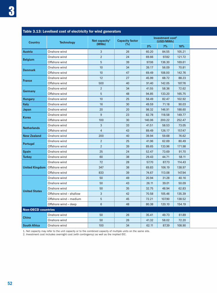
52

3

52

Table 3.13: Levelised cost of electricity for wind generators

Country Technology Net capacity1 (MWe)

Capacity factor (%)

Investment cost2 (USD/MWh)

Refurbishment and decom missioning costs (USD/MWh) O&M costs

(USD/MWh)

LCOE (USD/MWh) Country

3% 7% 10% 3% 7% 10% 3% 7% 10%

Austria Onshore wind 3 26 60.20 84.55 105.21 1.35 0.73 0.46 28.00 89.55 113.27 133.66 Austria

BelgiumOnshore wind 2 24 69.66 97.82 121.72 1.56 0.84 0.53 26.67 97.89 125.33 148.92

BelgiumOffshore wind 5 39 97.06 136.30 169.61 2.18 1.18 0.74 53.33 152.57 190.81 223.68

DenmarkOnshore wind 10 34 39.17 56.09 70.81 0.87 0.47 0.29 14.26 54.30 70.82 85.36

DenmarkOffshore wind 10 47 69.49 108.00 142.76 1.31 0.62 0.35 27.23 98.02 135.85 170.33

FranceOnshore wind 12 27 45.99 68.72 88.23 0.75 0.42 0.26 22.15 68.90 91.29 110.64

FranceOffshore wind 500 40 91.40 142.05 187.76 1.57 0.75 0.42 39.95 132.92 182.75 228.14

GermanyOnshore wind 2 34 41.55 58.36 72.62 0.93 0.50 0.32 34.67 77.15 93.53 107.60

GermanyOffshore wind 5 48 94.85 133.20 165.75 2.13 1.15 0.72 49.33 146.31 183.68 215.80

Hungary Onshore wind 10 25 58.49 82.47 102.92 2.97 1.87 1.30 32.31 93.77 116.65 136.54 Hungary

Italy Onshore wind 16 30 49.59 71.18 90.03 1.09 0.59 0.37 20.61 71.29 92.38 111.01 Italy

Japan Onshore wind 20 20 98.32 146.91 188.60 2.00 0.95 0.53 34.24 134.56 182.10 223.38 Japan

KoreaOnshore wind 9 23 82.78 118.58 149.77 0.00 0.00 0.00 28.86 111.64 147.45 178.63

KoreaOffshore wind 100 30 140.06 200.22 252.47 0.00 0.00 0.00 74.41 214.47 274.63 326.88

NetherlandsOnshore wind 3 33 41.51 58.53 73.05 0.29 0.16 0.10 26.26 68.06 84.94 99.40

NetherlandsOffshore wind 4 43 89.49 126.17 157.47 2.11 1.14 0.71 40.71 132.30 168.02 198.89

New Zealand Onshore wind 200 40 39.94 59.68 76.62 0.77 0.37 0.21 14.49 55.20 74.53 91.31 New Zealand

PortugalOnshore wind 2 25 41.96 62.69 80.49 0.81 0.39 0.22 18.26 61.03 81.34 98.97

PortugalOffshore wind 2 39 89.65 133.96 171.98 1.73 0.82 0.46 88.36 179.75 223.14 260.81

Spain Onshore wind 25 24 52.47 73.69 91.70 1.18 0.64 0.40 27.86 81.51 102.19 119.96 Spain

Turkey Onshore wind 60 38 29.43 44.71 58.11 8.67 7.10 5.95 21.38 59.48 73.19 85.43 Turkey

United Kingdom

Onshore wind 72 28 57.70 87.73 114.43 0.00 0.00 0.00 36.24 93.94 123.97 150.67

United KingdomOffshore wind 347 38 69.83 106.19 138.97 0.00 0.00 0.00 52.08 121.91 158.27 191.05

Offshore wind 833 39 74.67 113.08 147.94 0.00 0.00 0.00 61.15 135.82 174.23 209.09

United States

Onshore wind 50 49 20.94 31.28 40.16 0.41 0.19 0.11 11.37 32.71 42.85 51.64

United States

Onshore wind 50 43 26.11 39.01 50.09 0.51 0.24 0.13 12.98 39.60 52.23 63.20

Onshore wind 50 35 32.75 48.94 62.83 0.63 0.30 0.17 16.08 49.46 65.32 79.08

Offshore wind – shallow 3 42 70.58 105.46 135.39 1.22 0.58 0.33 31.15 102.95 137.19 166.87

Offshore wind – medium 5 45 72.21 107.90 138.52 1.25 0.59 0.33 28.88 102.34 137.37 167.73

Offshore wind – deep 6 48 80.38 120.10 154.19 1.39 0.66 0.37 33.81 115.58 154.58 188.38

Non-OECD countries Non-OECD countries

ChinaOnshore wind 50 26 35.41 49.73 61.89 0.79 0.43 0.27 9.76 45.96 59.92 71.91

ChinaOnshore wind 50 26 41.32 58.02 72.20 0.93 0.50 0.31 9.76 52.00 68.28 82.27

South Africa Onshore wind 100 34 62.11 87.39 108.90 1.26 0.68 0.43 13.86 77.24 101.93 123.19 South Africa

1. Net capacity may refer to the unit capacity or to the combined capacity of multiple units on the same site.2. Investment cost includes overnight cost (with contingency) as well as the implied IDC.

53

3

53

Table 3.13: Levelised cost of electricity for wind generators

Country Technology Net capacity1 (MWe)

Capacity factor (%)

Investment cost2 (USD/MWh)

Refurbishment and decom missioning costs (USD/MWh) O&M costs

(USD/MWh)

LCOE (USD/MWh) Country

3% 7% 10% 3% 7% 10% 3% 7% 10%

Austria Onshore wind 3 26 60.20 84.55 105.21 1.35 0.73 0.46 28.00 89.55 113.27 133.66 Austria

BelgiumOnshore wind 2 24 69.66 97.82 121.72 1.56 0.84 0.53 26.67 97.89 125.33 148.92

BelgiumOffshore wind 5 39 97.06 136.30 169.61 2.18 1.18 0.74 53.33 152.57 190.81 223.68

DenmarkOnshore wind 10 34 39.17 56.09 70.81 0.87 0.47 0.29 14.26 54.30 70.82 85.36

DenmarkOffshore wind 10 47 69.49 108.00 142.76 1.31 0.62 0.35 27.23 98.02 135.85 170.33

FranceOnshore wind 12 27 45.99 68.72 88.23 0.75 0.42 0.26 22.15 68.90 91.29 110.64

FranceOffshore wind 500 40 91.40 142.05 187.76 1.57 0.75 0.42 39.95 132.92 182.75 228.14

GermanyOnshore wind 2 34 41.55 58.36 72.62 0.93 0.50 0.32 34.67 77.15 93.53 107.60

GermanyOffshore wind 5 48 94.85 133.20 165.75 2.13 1.15 0.72 49.33 146.31 183.68 215.80

Hungary Onshore wind 10 25 58.49 82.47 102.92 2.97 1.87 1.30 32.31 93.77 116.65 136.54 Hungary

Italy Onshore wind 16 30 49.59 71.18 90.03 1.09 0.59 0.37 20.61 71.29 92.38 111.01 Italy

Japan Onshore wind 20 20 98.32 146.91 188.60 2.00 0.95 0.53 34.24 134.56 182.10 223.38 Japan

KoreaOnshore wind 9 23 82.78 118.58 149.77 0.00 0.00 0.00 28.86 111.64 147.45 178.63

KoreaOffshore wind 100 30 140.06 200.22 252.47 0.00 0.00 0.00 74.41 214.47 274.63 326.88

NetherlandsOnshore wind 3 33 41.51 58.53 73.05 0.29 0.16 0.10 26.26 68.06 84.94 99.40

NetherlandsOffshore wind 4 43 89.49 126.17 157.47 2.11 1.14 0.71 40.71 132.30 168.02 198.89

New Zealand Onshore wind 200 40 39.94 59.68 76.62 0.77 0.37 0.21 14.49 55.20 74.53 91.31 New Zealand

PortugalOnshore wind 2 25 41.96 62.69 80.49 0.81 0.39 0.22 18.26 61.03 81.34 98.97

PortugalOffshore wind 2 39 89.65 133.96 171.98 1.73 0.82 0.46 88.36 179.75 223.14 260.81

Spain Onshore wind 25 24 52.47 73.69 91.70 1.18 0.64 0.40 27.86 81.51 102.19 119.96 Spain

Turkey Onshore wind 60 38 29.43 44.71 58.11 8.67 7.10 5.95 21.38 59.48 73.19 85.43 Turkey

United Kingdom

Onshore wind 72 28 57.70 87.73 114.43 0.00 0.00 0.00 36.24 93.94 123.97 150.67

United KingdomOffshore wind 347 38 69.83 106.19 138.97 0.00 0.00 0.00 52.08 121.91 158.27 191.05

Offshore wind 833 39 74.67 113.08 147.94 0.00 0.00 0.00 61.15 135.82 174.23 209.09

United States

Onshore wind 50 49 20.94 31.28 40.16 0.41 0.19 0.11 11.37 32.71 42.85 51.64

United States

Onshore wind 50 43 26.11 39.01 50.09 0.51 0.24 0.13 12.98 39.60 52.23 63.20

Onshore wind 50 35 32.75 48.94 62.83 0.63 0.30 0.17 16.08 49.46 65.32 79.08

Offshore wind – shallow 3 42 70.58 105.46 135.39 1.22 0.58 0.33 31.15 102.95 137.19 166.87

Offshore wind – medium 5 45 72.21 107.90 138.52 1.25 0.59 0.33 28.88 102.34 137.37 167.73

Offshore wind – deep 6 48 80.38 120.10 154.19 1.39 0.66 0.37 33.81 115.58 154.58 188.38

Non-OECD countries Non-OECD countries

ChinaOnshore wind 50 26 35.41 49.73 61.89 0.79 0.43 0.27 9.76 45.96 59.92 71.91

ChinaOnshore wind 50 26 41.32 58.02 72.20 0.93 0.50 0.31 9.76 52.00 68.28 82.27

South Africa Onshore wind 100 34 62.11 87.39 108.90 1.26 0.68 0.43 13.86 77.24 101.93 123.19 South Africa

1. Net capacity may refer to the unit capacity or to the combined capacity of multiple units on the same site.2. Investment cost includes overnight cost (with contingency) as well as the implied IDC.

54

3

54

Table 3.14: Levelised cost of electricity for other renewable generation

Country Technology Net capacity1 (MWe)

Capacity factor (%)

Investment cost2 (USD/MWh)

Refurbishment and decom­missioning costs (USD/MWh)

Fuel and waste costs (USD/MWh)

Carbon cost (USD/MWh)

O&M costs (USD/MWh)

LCOE (USD/MWh) Country

3% 7% 10% 3% 7% 10% 3% 7% 10%

Austria Small hydro – run-of-river 2.2 51 23.97 57.48 89.66 0.08 0.01 0.00 0.00 0.00 26.65 50.70 84.14 116.31 Austria

GermanySmall hydro – run-of-river 2 55 77.20 171.90 265.40 0.48 0.08 0.02 0.00 0.00 41.10 118.78 213.08 306.51

GermanyLarge hydro – run-of-river 20 63 47.40 105.72 163.40 0.29 0.05 0.01 0.00 0.00 17.40 65.08 123.16 180.80

Italy

Biogas – engine 0.3 80 84.43 121.02 152.88 1.86 1.01 0.63 63.42 0.00 63.36 213.07 248.80 280.29

Italy

Solid biomass – turbine 0.199 86 63.03 90.53 114.54 1.39 0.75 0.47 156.89 0.00 69.82 291.12 317.98 341.71

Solid waste incineration3 10 84 53.65 76.82 96.98 1.19 0.64 0.40 -90.67 0.00 192.75 156.92 179.55 199.47

Small hydro – run-of-river 0.396 49 94.70 136.51 173.20 2.08 1.12 0.70 0.00 0.00 35.30 132.08 172.94 209.20

Geothermal 20 92 40.89 62.30 81.14 0.78 0.37 0.21 0.00 0.00 18.20 59.87 80.87 99.55

Japan Large hydro 12 45 79.87 191.56 298.81 0.29 0.02 0.00 0.00 0.00 22.57 102.74 214.16 321.39 Japan

NetherlandsSolid waste incineration 19.8 85 23.89 38.59 51.65 0.41 0.17 0.09 0.00 11.40 16.00 51.70 66.16 79.14

NetherlandsCo-firing of wood pellets 640 80 4.35 7.06 9.47 0.08 0.03 0.02 96.26 12.00 4.00 116.69 119.34 121.74

New Zealand Geothermal 250 89 20.29 34.34 46.78 0.29 0.10 0.05 0.00 0.00 11.31 31.90 45.76 58.14 New Zealand

PortugalLarge hydro – reservoir 144 17 72.59 171.53 267.17 0.29 0.03 0.00 0.00 0.00 16.65 89.54 188.22 283.83

PortugalLarge hydro – pumped storage 218 28 56.09 132.55 206.45 0.23 0.02 0.00 0.00 0.00 12.14 68.46 144.71 218.59

Spain

Biomass – turbine 10 75 36.56 56.83 75.11 0.69 0.33 0.18 73.41 0.00 41.22 151.88 171.78 189.93

Spain

Biogas – engine 1 48 25.29 37.80 48.52 0.49 0.23 0.13 0.00 0.00 52.13 77.92 90.16 100.79

Biogas – engine 1.5 48 50.99 76.19 97.82 0.99 0.47 0.26 0.00 0.00 60.52 112.49 137.17 158.60

Solid waste incineration – turbine 15 56 103.00 160.09 211.61 1.93 0.92 0.52 0.00 0.00 124.34 229.28 285.34 336.46

Small hydro – run-of-river 2 39 44.82 69.66 92.08 0.84 0.40 0.22 0.00 0.00 38.40 84.06 108.46 130.70

Small hydro – reservoir 2 40 27.77 42.31 55.11 0.53 0.25 0.14 0.00 0.00 38.40 66.70 80.96 93.65

Large hydro – run-of-river 20 39 32.19 50.03 66.13 0.60 0.29 0.16 0.00 0.00 32.40 65.20 82.72 98.70

Large hydro – reservoir 20 40 19.97 30.43 39.63 0.38 0.18 0.10 0.00 0.00 0.00 20.35 30.61 39.73

Switzerland

Small hydro – run-of-river 10 54 52.47 125.84 196.29 0.18 0.02 0.00 0.00 0.00 21.83 74.48 147.68 218.12

SwitzerlandLarge hydro – run-of-river 50 50 51.18 122.75 191.47 0.18 0.01 0.00 0.00 0.00 10.17 61.53 132.94 201.65

Large hydro – reservoir 50 28 101.82 244.19 380.91 0.35 0.03 0.00 0.00 0.00 7.53 109.71 251.75 388.45

Large hydro – pumped storage 1 000 26 25.95 62.23 97.07 0.09 0.01 0.00 0.00 0.00 9.54 35.58 71.78 106.61

TurkeyGeothermal 24 90 9.23 16.28 22.87 0.13 0.05 0.02 0.00 0.00 100.00 109.36 116.33 122.89

TurkeyLarge hydro – reservoir 19 54 17.38 33.72 48.36 8.02 2.74 1.17 0.00 0.00 4.88 30.28 41.34 54.41

United Kingdom

Biomass 900 65 7.95 11.52 14.58 0.17 0.09 0.05 134.68 0.00 21.10 163.90 167.38 170.41

United KingdomLarge hydro 11 35 74.49 133.89 186.78 0.00 0.00 0.00 0.00 0.00 41.02 115.52 174.91 227.80

Geothermal 6.8 91 50.02 79.45 106.68 0.92 0.44 0.25 0.00 0.00 37.09 88.03 116.98 144.01

United States

Biomass 100 85 32.37 53.16 72.03 0.52 0.22 0.11 51.80 0.00 14.46 99.15 119.64 138.39

United States

Hydro – non-power dams 0.1 65 10.21 21.50 32.81 0.09 0.02 0.01 0.00 0.00 5.08 15.38 26.60 37.90

Hydro – non-power dams 3 62 39.36 82.88 126.46 0.33 0.08 0.02 0.00 0.00 5.19 44.89 88.15 131.68

Hydro – non-power dams 8 58 75.90 159.81 243.87 0.64 0.15 0.04 0.00 0.00 5.37 81.90 165.33 249.28

Hydro – new stream development 10 68 25.64 54.00 82.40 0.22 0.05 0.02 0.00 0.00 4.99 30.85 59.04 87.40

Hydro – new stream development 20 66 40.93 86.19 131.52 0.35 0.08 0.02 0.00 0.00 5.06 46.34 91.34 136.61

Hydro – new stream development 30 62 58.78 123.76 188.85 0.50 0.11 0.03 0.00 0.00 5.19 64.47 129.07 194.08

Geothermal – flash steam 20 90 39.36 63.39 84.65 0.65 0.27 0.13 0.00 0.00 14.54 54.54 78.20 99.33

Geothermal – binary rankine cycle 20 80 46.49 74.87 99.99 0.76 0.32 0.16 0.00 0.00 16.35 63.61 91.54 116.50

Non-OECD countries Non-OECD countries

Brazil

Large hydro – run-of-river 15 57 42.04 69.56 94.79 0.68 0.28 0.14 0.00 0.00 8.89 51.60 78.74 103.82

BrazilLarge hydro 270 56 13.22 26.29 38.40 0.12 0.03 0.01 0.00 0.00 8.94 22.28 35.26 47.35

Large hydro – run-of-river 800 55 13.24 26.22 38.20 0.10 0.02 0.01 0.00 0.00 9.00 22.34 35.25 47.21

Large hydro – run-of-river 1 800 52 10.53 21.51 32.06 0.09 0.02 0.01 0.00 0.00 9.18 19.79 30.71 41.24

China Large hydro – reservoir 13 050 52 4.76 11.43 17.82 0.02 0.00 0.00 0.00 0.00 10.57 15.35 22.00 28.39 China1. Net capacity may refer to the unit capacity or to the combined capacity of multiple units on the same site.2. Investment cost includes overnight cost (with contingency) as well as the implied IDC.

3. Fuel costs for Italy’s solid waste incineration are negative because it includes an assumed feed-in tariff, which is considered a source of revenue for this plant.

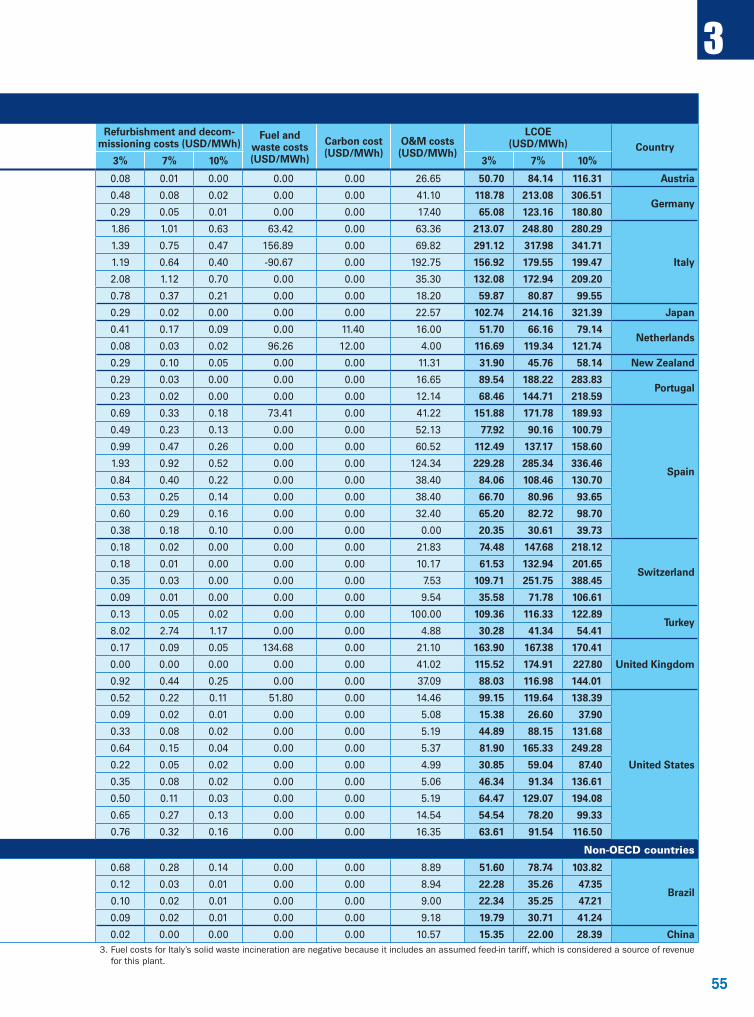
55

3

55

Table 3.14: Levelised cost of electricity for other renewable generation

Country Technology Net capacity1 (MWe)

Capacity factor (%)

Investment cost2 (USD/MWh)

Refurbishment and decom­missioning costs (USD/MWh)

Fuel and waste costs (USD/MWh)

Carbon cost (USD/MWh)

O&M costs (USD/MWh)

LCOE (USD/MWh) Country

3% 7% 10% 3% 7% 10% 3% 7% 10%

Austria Small hydro – run-of-river 2.2 51 23.97 57.48 89.66 0.08 0.01 0.00 0.00 0.00 26.65 50.70 84.14 116.31 Austria

GermanySmall hydro – run-of-river 2 55 77.20 171.90 265.40 0.48 0.08 0.02 0.00 0.00 41.10 118.78 213.08 306.51

GermanyLarge hydro – run-of-river 20 63 47.40 105.72 163.40 0.29 0.05 0.01 0.00 0.00 17.40 65.08 123.16 180.80

Italy

Biogas – engine 0.3 80 84.43 121.02 152.88 1.86 1.01 0.63 63.42 0.00 63.36 213.07 248.80 280.29

Italy

Solid biomass – turbine 0.199 86 63.03 90.53 114.54 1.39 0.75 0.47 156.89 0.00 69.82 291.12 317.98 341.71

Solid waste incineration3 10 84 53.65 76.82 96.98 1.19 0.64 0.40 -90.67 0.00 192.75 156.92 179.55 199.47

Small hydro – run-of-river 0.396 49 94.70 136.51 173.20 2.08 1.12 0.70 0.00 0.00 35.30 132.08 172.94 209.20

Geothermal 20 92 40.89 62.30 81.14 0.78 0.37 0.21 0.00 0.00 18.20 59.87 80.87 99.55

Japan Large hydro 12 45 79.87 191.56 298.81 0.29 0.02 0.00 0.00 0.00 22.57 102.74 214.16 321.39 Japan

NetherlandsSolid waste incineration 19.8 85 23.89 38.59 51.65 0.41 0.17 0.09 0.00 11.40 16.00 51.70 66.16 79.14

NetherlandsCo-firing of wood pellets 640 80 4.35 7.06 9.47 0.08 0.03 0.02 96.26 12.00 4.00 116.69 119.34 121.74

New Zealand Geothermal 250 89 20.29 34.34 46.78 0.29 0.10 0.05 0.00 0.00 11.31 31.90 45.76 58.14 New Zealand

PortugalLarge hydro – reservoir 144 17 72.59 171.53 267.17 0.29 0.03 0.00 0.00 0.00 16.65 89.54 188.22 283.83

PortugalLarge hydro – pumped storage 218 28 56.09 132.55 206.45 0.23 0.02 0.00 0.00 0.00 12.14 68.46 144.71 218.59

Spain

Biomass – turbine 10 75 36.56 56.83 75.11 0.69 0.33 0.18 73.41 0.00 41.22 151.88 171.78 189.93

Spain

Biogas – engine 1 48 25.29 37.80 48.52 0.49 0.23 0.13 0.00 0.00 52.13 77.92 90.16 100.79

Biogas – engine 1.5 48 50.99 76.19 97.82 0.99 0.47 0.26 0.00 0.00 60.52 112.49 137.17 158.60

Solid waste incineration – turbine 15 56 103.00 160.09 211.61 1.93 0.92 0.52 0.00 0.00 124.34 229.28 285.34 336.46

Small hydro – run-of-river 2 39 44.82 69.66 92.08 0.84 0.40 0.22 0.00 0.00 38.40 84.06 108.46 130.70

Small hydro – reservoir 2 40 27.77 42.31 55.11 0.53 0.25 0.14 0.00 0.00 38.40 66.70 80.96 93.65

Large hydro – run-of-river 20 39 32.19 50.03 66.13 0.60 0.29 0.16 0.00 0.00 32.40 65.20 82.72 98.70

Large hydro – reservoir 20 40 19.97 30.43 39.63 0.38 0.18 0.10 0.00 0.00 0.00 20.35 30.61 39.73

Switzerland

Small hydro – run-of-river 10 54 52.47 125.84 196.29 0.18 0.02 0.00 0.00 0.00 21.83 74.48 147.68 218.12

SwitzerlandLarge hydro – run-of-river 50 50 51.18 122.75 191.47 0.18 0.01 0.00 0.00 0.00 10.17 61.53 132.94 201.65

Large hydro – reservoir 50 28 101.82 244.19 380.91 0.35 0.03 0.00 0.00 0.00 7.53 109.71 251.75 388.45

Large hydro – pumped storage 1 000 26 25.95 62.23 97.07 0.09 0.01 0.00 0.00 0.00 9.54 35.58 71.78 106.61

TurkeyGeothermal 24 90 9.23 16.28 22.87 0.13 0.05 0.02 0.00 0.00 100.00 109.36 116.33 122.89

TurkeyLarge hydro – reservoir 19 54 17.38 33.72 48.36 8.02 2.74 1.17 0.00 0.00 4.88 30.28 41.34 54.41

United Kingdom

Biomass 900 65 7.95 11.52 14.58 0.17 0.09 0.05 134.68 0.00 21.10 163.90 167.38 170.41

United KingdomLarge hydro 11 35 74.49 133.89 186.78 0.00 0.00 0.00 0.00 0.00 41.02 115.52 174.91 227.80

Geothermal 6.8 91 50.02 79.45 106.68 0.92 0.44 0.25 0.00 0.00 37.09 88.03 116.98 144.01

United States

Biomass 100 85 32.37 53.16 72.03 0.52 0.22 0.11 51.80 0.00 14.46 99.15 119.64 138.39

United States

Hydro – non-power dams 0.1 65 10.21 21.50 32.81 0.09 0.02 0.01 0.00 0.00 5.08 15.38 26.60 37.90

Hydro – non-power dams 3 62 39.36 82.88 126.46 0.33 0.08 0.02 0.00 0.00 5.19 44.89 88.15 131.68

Hydro – non-power dams 8 58 75.90 159.81 243.87 0.64 0.15 0.04 0.00 0.00 5.37 81.90 165.33 249.28

Hydro – new stream development 10 68 25.64 54.00 82.40 0.22 0.05 0.02 0.00 0.00 4.99 30.85 59.04 87.40

Hydro – new stream development 20 66 40.93 86.19 131.52 0.35 0.08 0.02 0.00 0.00 5.06 46.34 91.34 136.61

Hydro – new stream development 30 62 58.78 123.76 188.85 0.50 0.11 0.03 0.00 0.00 5.19 64.47 129.07 194.08

Geothermal – flash steam 20 90 39.36 63.39 84.65 0.65 0.27 0.13 0.00 0.00 14.54 54.54 78.20 99.33

Geothermal – binary rankine cycle 20 80 46.49 74.87 99.99 0.76 0.32 0.16 0.00 0.00 16.35 63.61 91.54 116.50

Non-OECD countries Non-OECD countries

Brazil

Large hydro – run-of-river 15 57 42.04 69.56 94.79 0.68 0.28 0.14 0.00 0.00 8.89 51.60 78.74 103.82

BrazilLarge hydro 270 56 13.22 26.29 38.40 0.12 0.03 0.01 0.00 0.00 8.94 22.28 35.26 47.35

Large hydro – run-of-river 800 55 13.24 26.22 38.20 0.10 0.02 0.01 0.00 0.00 9.00 22.34 35.25 47.21

Large hydro – run-of-river 1 800 52 10.53 21.51 32.06 0.09 0.02 0.01 0.00 0.00 9.18 19.79 30.71 41.24

China Large hydro – reservoir 13 050 52 4.76 11.43 17.82 0.02 0.00 0.00 0.00 0.00 10.57 15.35 22.00 28.39 China1. Net capacity may refer to the unit capacity or to the combined capacity of multiple units on the same site.2. Investment cost includes overnight cost (with contingency) as well as the implied IDC.

3. Fuel costs for Italy’s solid waste incineration are negative because it includes an assumed feed-in tariff, which is considered a source of revenue for this plant.

56

3

56

Table 3.15: Levelised cost of electricity for combined heat and power plants

Country Technology Net capacity (MWe)

Capacity factor (%)

Investment cost1 (USD/MWh)

Refurbishment and decom­missioning costs (USD/MWh)

Fuel and waste costs (USD/MWh)

Carbon cost

(USD/MWh)

O&M costs

(USD/MWh)

Heat credit

(USD/MWh)

LCOE (USD/MWh) Country

3% 7% 10% 3% 7% 10% 3% 7% 10%

AustriaSolid biomass 2 80 39.45 63.55 84.86 0.65 0.27 0.14 60.61 0.00 75.43 -96.43 79.71 103.42 124.60

AustriaBiogas 0.5 91 38.84 62.56 83.54 0.64 0.26 0.13 82.42 0.00 27.67 -33.75 115.82 139.16 160.01

Denmark

Medium – wood chips 1 46 77.51 132.61 185.31 1.22 0.51 0.25 119.55 0.00 15.93 -85.19 129.01 183.40 235.86

Denmark

Medium – straw 1 46 87.24 141.20 192.46 1.59 0.75 0.42 103.46 0.00 23.38 -79.66 136.01 189.14 240.06

Medium – natural gas 1 46 13.49 20.56 26.78 0.26 0.12 0.07 94.68 15.32 4.63 -33.69 94.69 101.63 107.79

Large – wood pellets 1 57 31.23 58.65 84.88 0.37 0.11 0.04 119.54 0.00 21.79 -33.06 139.87 167.04 193.20

Large – coal 1 49 31.23 58.65 84.88 0.37 0.11 0.04 32.55 25.63 21.79 -33.06 78.51 105.68 131.84

Large – natural gas 1 57 15.56 23.70 30.87 0.30 0.14 0.08 71.46 11.56 12.75 -18.40 93.22 101.21 108.32

Germany

Engine – biogas (digester) 0.5 80 19.26 27.19 33.97 16.01 23.09 28.80 0.00 0.00 32.93 -43.20 25.00 40.01 52.50

Germany

Engine – biogas 0.2 63 31.42 44.42 55.55 20.21 36.00 47.83 0.00 0.00 59.74 -51.75 59.62 88.40 111.37

Engine – mine gas 1.5 80 11.98 16.90 21.11 10.08 14.84 18.64 0.00 0.00 28.55 -46.20 4.40 14.09 22.10

Steam turbine – solid biomass 4 68 79.59 113.98 143.89 1.76 0.95 0.59 106.88 0.00 41.11 -150.75 78.59 112.16 141.72

Geothermal 3.3 73 182.87 288.10 391.39 3.77 2.03 1.27 0.00 0.00 77.58 -31.36 232.86 336.35 438.88

NetherlandsBiogas/fermentation 3 85 20.13 25.80 30.59 0.59 0.39 0.28 95.29 9.90 13.97 -31.43 108.46 113.93 118.60

NetherlandsBiogas/fermentation 1.1 85 22.14 28.38 33.64 0.65 0.43 0.31 124.39 9.90 15.22 -31.65 140.66 146.67 151.82

SpainEngine 4.7 63 92.61 143.94 190.26 1.74 0.83 0.46 63.74 6.03 36.29 -41.17 159.25 209.66 255.62

SpainGas turbine 4.9 71 14.03 21.37 27.83 0.27 0.13 0.07 59.66 6.03 31.40 -82.46 28.92 36.12 42.53

United KingdomBiomass 62 83 48.52 75.82 100.61 0.91 0.43 0.24 185.39 0.00 55.93 -45.00 245.75 272.57 297.17

United KingdomGeothermal 6.8 91 54.73 86.92 116.70 1.01 0.48 0.27 0.00 0.00 40.96 -45.00 51.70 83.36 112.92

1. Investment cost includes overnight cost (with contingency) as well as the implied IDC.

3.3 Capacity factor sensitivity of baseload technologies

Natural gas, coal and nuclear plants in this report were all modelled under an assumed capacity factor of 85%, even when differing national assumptions were provided. However, actual capacity factors will depend on many country-specific factors, including relative fuel cost and the penetration of variable renewable power. Many plants that are considered “baseload” will in fact operate at lower capacity factors under actual operating conditions. As noted above, reported capacity factors for nuclear plants were 82.4% in 2013. In the data provided for the purpose of this report, capacity factors for CCGTs ranged from a low of 35% to a high of 93%, and for coal plants from 52% to 91%.

Chapter 11 discusses in more detail the relevance of LCOE as a measure in an environment where “baseload” as a concept has less meaning. In addition, a 50% capacity factor sensitivity is included for all of the baseload technologies. The results are presented in Tables 3.16 to 3.18, alongside the LCOEs calculated at an 85% capacity factor, which was presented above.

The sensitivity of a given technology to capacity factor is determined by its ratio of capital to operating costs. Further, the capacity factor under operations is an economic decision, taken on the basis of a combination of the generating unit’s marginal cost, the market price/avoided cost at the time of production, generator availability, and inter-temporal (start-up and ramping) and system constraints. Units with high capital to operating cost ratios are generally run at higher capacity factors, because there are many hours where their marginal costs are lower than other units. Conversely, units with high operating to capital costs are run at lower capacity factors, because there are relatively few hours where their marginal costs are lower than other units.

57

3

57

Table 3.15: Levelised cost of electricity for combined heat and power plants

Country Technology Net capacity (MWe)

Capacity factor (%)

Investment cost1 (USD/MWh)

Refurbishment and decom­missioning costs (USD/MWh)

Fuel and waste costs (USD/MWh)

Carbon cost

(USD/MWh)

O&M costs

(USD/MWh)

Heat credit

(USD/MWh)

LCOE (USD/MWh) Country

3% 7% 10% 3% 7% 10% 3% 7% 10%

AustriaSolid biomass 2 80 39.45 63.55 84.86 0.65 0.27 0.14 60.61 0.00 75.43 -96.43 79.71 103.42 124.60

AustriaBiogas 0.5 91 38.84 62.56 83.54 0.64 0.26 0.13 82.42 0.00 27.67 -33.75 115.82 139.16 160.01

Denmark

Medium – wood chips 1 46 77.51 132.61 185.31 1.22 0.51 0.25 119.55 0.00 15.93 -85.19 129.01 183.40 235.86

Denmark

Medium – straw 1 46 87.24 141.20 192.46 1.59 0.75 0.42 103.46 0.00 23.38 -79.66 136.01 189.14 240.06

Medium – natural gas 1 46 13.49 20.56 26.78 0.26 0.12 0.07 94.68 15.32 4.63 -33.69 94.69 101.63 107.79

Large – wood pellets 1 57 31.23 58.65 84.88 0.37 0.11 0.04 119.54 0.00 21.79 -33.06 139.87 167.04 193.20

Large – coal 1 49 31.23 58.65 84.88 0.37 0.11 0.04 32.55 25.63 21.79 -33.06 78.51 105.68 131.84

Large – natural gas 1 57 15.56 23.70 30.87 0.30 0.14 0.08 71.46 11.56 12.75 -18.40 93.22 101.21 108.32

Germany

Engine – biogas (digester) 0.5 80 19.26 27.19 33.97 16.01 23.09 28.80 0.00 0.00 32.93 -43.20 25.00 40.01 52.50

Germany

Engine – biogas 0.2 63 31.42 44.42 55.55 20.21 36.00 47.83 0.00 0.00 59.74 -51.75 59.62 88.40 111.37

Engine – mine gas 1.5 80 11.98 16.90 21.11 10.08 14.84 18.64 0.00 0.00 28.55 -46.20 4.40 14.09 22.10

Steam turbine – solid biomass 4 68 79.59 113.98 143.89 1.76 0.95 0.59 106.88 0.00 41.11 -150.75 78.59 112.16 141.72

Geothermal 3.3 73 182.87 288.10 391.39 3.77 2.03 1.27 0.00 0.00 77.58 -31.36 232.86 336.35 438.88

NetherlandsBiogas/fermentation 3 85 20.13 25.80 30.59 0.59 0.39 0.28 95.29 9.90 13.97 -31.43 108.46 113.93 118.60

NetherlandsBiogas/fermentation 1.1 85 22.14 28.38 33.64 0.65 0.43 0.31 124.39 9.90 15.22 -31.65 140.66 146.67 151.82

SpainEngine 4.7 63 92.61 143.94 190.26 1.74 0.83 0.46 63.74 6.03 36.29 -41.17 159.25 209.66 255.62

SpainGas turbine 4.9 71 14.03 21.37 27.83 0.27 0.13 0.07 59.66 6.03 31.40 -82.46 28.92 36.12 42.53

United KingdomBiomass 62 83 48.52 75.82 100.61 0.91 0.43 0.24 185.39 0.00 55.93 -45.00 245.75 272.57 297.17

United KingdomGeothermal 6.8 91 54.73 86.92 116.70 1.01 0.48 0.27 0.00 0.00 40.96 -45.00 51.70 83.36 112.92

1. Investment cost includes overnight cost (with contingency) as well as the implied IDC.

It is important to note that 50% was not chosen as an indication that such capacity factors are expected to be typical in the future. In particular, the specific nature of current nuclear power technologies makes a 50% capacity factor unrealistic for reasons that extend beyond economics. A 50% capacity factor was chosen because it is far enough from 85% to show the impact on LCOE without being so low as to present results that are unreasonable under any circumstances.

For that reason, it is important to bear in mind that the 50% capacity factor results do not necessarily represent the expected LCOEs for these technologies in 2020. They are presented merely to show how sensitive these technologies are to changes in operating conditions. This topic is also explored in the median case sensitivity analysis presented in Chapter 7.

It should also be noted that the efficiency of the plants was not adjusted as part of this sensitivity. Efficiency would decline for all technologies at lower capacity factors, though the impact would be small. These results are therefore relatively optimistic relative to what actual LCOEs would be under these operating conditions.

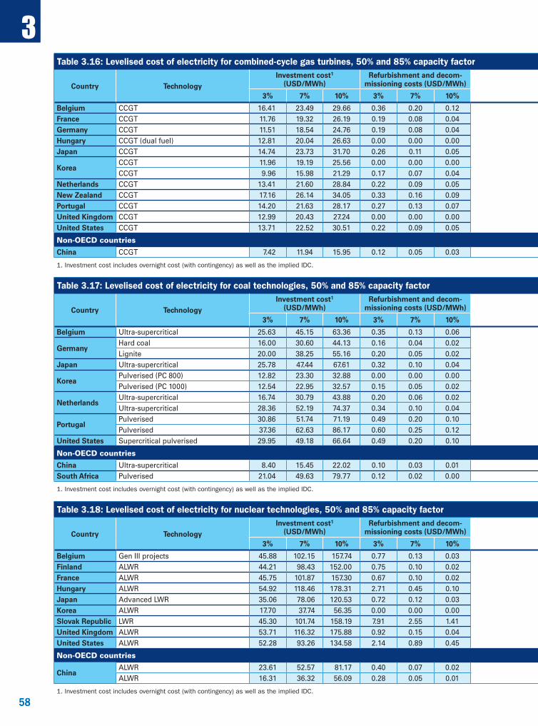
58

3

58

Table 3.16: Levelised cost of electricity for combined-cycle gas turbines, 50% and 85% capacity factor

Country TechnologyInvestment cost1

(USD/MWh)Refurbishment and decom­

missioning costs (USD/MWh)Fuel and

waste costs (USD/MWh)

Carbon cost

(USD/MWh)

O&M costs

(USD/MWh)

LCOE at 50% capacity factor (USD/MWh)

LCOE at 85% capacity factor (USD/MWh) Country

3% 7% 10% 3% 7% 10% 3% 7% 10% 3% 7% 10%

Belgium CCGT 16.41 23.49 29.66 0.36 0.20 0.12 74.62 10.08 5.35 106.82 113.74 119.83 98.54 102.61 106.19 BelgiumFrance CCGT 11.76 19.32 26.19 0.19 0.08 0.04 68.99 10.56 8.75 100.26 107.71 114.53 92.83 97.21 101.23 FranceGermany CCGT 11.51 18.54 24.76 0.19 0.08 0.04 74.00 9.90 11.22 106.82 113.74 119.92 98.49 102.56 106.20 GermanyHungary CCGT (dual fuel) 12.81 20.04 26.63 0.00 0.00 0.00 71.21 10.56 11.59 106.16 113.40 119.99 96.94 101.20 105.08 HungaryJapan CCGT 14.74 23.73 31.70 0.26 0.11 0.05 104.07 10.95 13.88 143.88 152.73 160.64 133.21 138.42 143.07 Japan

KoreaCCGT 11.96 19.19 25.56 0.00 0.00 0.00 98.97 10.27 9.43 130.63 137.86 144.24 121.82 126.08 129.82

KoreaCCGT 9.96 15.98 21.29 0.17 0.07 0.04 95.21 9.89 6.89 122.12 128.05 133.32 115.11 118.60 121.70

Netherlands CCGT 13.41 21.60 28.84 0.22 0.09 0.05 75.25 9.90 5.36 104.15 112.21 119.40 96.71 101.45 105.68 NetherlandsNew Zealand CCGT 17.16 26.14 34.05 0.33 0.16 0.09 46.75 11.22 10.07 85.53 94.35 102.19 75.64 80.82 85.43 New ZealandPortugal CCGT 14.20 21.63 28.17 0.27 0.13 0.07 74.00 9.90 7.62 105.98 113.27 119.76 98.65 102.93 106.75 PortugalUnited Kingdom CCGT 12.99 20.43 27.24 0.00 0.00 0.00 75.51 9.43 11.15 109.09 116.53 123.34 99.21 103.59 107.59 United KingdomUnited States CCGT 13.71 22.52 30.51 0.22 0.09 0.05 36.90 11.10 6.13 68.07 76.74 84.69 60.84 65.95 70.62 United States

Non-OECD countries Non-OECD countriess

China CCGT 7.42 11.94 15.95 0.12 0.05 0.03 71.47 11.02 3.25 93.27 97.73 101.71 90.17 92.79 95.13 China

1. Investment cost includes overnight cost (with contingency) as well as the implied IDC.

Table 3.17: Levelised cost of electricity for coal technologies, 50% and 85% capacity factor

Country TechnologyInvestment cost1

(USD/MWh)Refurbishment and decom­

missioning costs (USD/MWh)Fuel and

waste costs (USD/MWh)

Carbon cost

(USD/MWh)

O&M costs

(USD/MWh)

LCOE at 50% capacity factor (USD/MWh)

LCOE at 85% capacity factor (USD/MWh) Country

3% 7% 10% 3% 7% 10% 3% 7% 10% 3% 7% 10%

Belgium Ultra-supercritical 25.63 45.15 63.36 0.35 0.13 0.06 26.67 22.05 12.01 86.72 106.00 124.14 72.00 83.35 94.02 Belgium

GermanyHard coal 16.00 30.60 44.13 0.16 0.04 0.02 26.38 21.98 13.66 78.18 92.66 106.16 67.01 75.53 83.47

GermanyLignite 20.00 38.25 55.16 0.20 0.05 0.02 14.88 28.20 16.46 79.75 97.85 114.73 66.04 76.69 86.61

Japan Ultra-supercritical 25.78 47.44 67.61 0.32 0.10 0.04 35.91 25.02 27.19 114.22 135.66 155.77 94.81 107.42 119.25 Japan

KoreaPulverised (PC 800) 12.82 23.30 32.88 0.00 0.00 0.00 40.04 24.77 9.03 86.66 97.14 106.72 77.66 83.83 89.46

KoreaPulverised (PC 1000) 12.54 22.95 32.57 0.15 0.05 0.02 38.36 23.67 8.16 82.89 93.20 102.78 74.30 80.36 86.00

NetherlandsUltra-supercritical 16.74 30.79 43.88 0.20 0.06 0.02 31.49 21.90 12.01 82.34 96.26 109.31 72.23 80.42 88.09

NetherlandsUltra-supercritical 28.36 52.19 74.37 0.34 0.10 0.04 31.49 21.90 12.01 94.10 117.70 139.82 79.15 93.03 106.04

PortugalPulverised 30.86 51.74 71.19 0.49 0.20 0.10 31.47 22.21 7.30 92.34 112.92 132.27 78.28 90.39 101.77

PortugalPulverised 37.36 62.63 86.17 0.60 0.25 0.12 28.38 20.03 15.83 102.20 127.12 150.54 85.27 99.93 113.71

United States Supercritical pulverised 29.95 49.18 66.64 0.49 0.20 0.10 28.42 25.20 17.06 101.12 120.07 137.42 82.64 93.79 104.00 United States

Non-OECD countries Non-OECD countriess

China Ultra-supercritical 8.40 15.45 22.02 0.10 0.03 0.01 35.67 28.88 4.07 77.10 84.09 90.64 73.61 77.72 81.57 ChinaSouth Africa Pulverised 21.04 49.63 79.77 0.12 0.02 0.00 20.45 27.00 7.74 76.36 104.85 134.97 65.31 82.07 99.79 South Africa

1. Investment cost includes overnight cost (with contingency) as well as the implied IDC.

Table 3.18: Levelised cost of electricity for nuclear technologies, 50% and 85% capacity factor

Country TechnologyInvestment cost1

(USD/MWh)Refurbishment and decom­

missioning costs (USD/MWh)Fuel and

waste costs (USD/MWh)

O&M costs

(USD/MWh)

LCOE at 50% capacity factor (USD/MWh)

LCOE at 85% capacity factor (USD/MWh) Country

3% 7% 10% 3% 7% 10% 3% 7% 10% 3% 7% 10%

Belgium Gen III projects 45.88 102.15 157.74 0.77 0.13 0.03 10.46 13.55 70.67 126.29 181.78 51.45 84.17 116.81 BelgiumFinland ALWR 44.21 98.43 152.00 0.75 0.10 0.02 5.09 14.59 64.65 118.21 171.70 46.13 77.64 109.10 FinlandFrance ALWR 45.75 101.87 157.30 0.67 0.10 0.02 9.33 13.33 69.09 124.63 179.98 49.98 82.64 115.21 FranceHungary ALWR 54.92 118.46 178.31 2.71 0.45 0.10 9.60 14.46 81.68 142.97 202.47 53.90 89.94 124.95 HungaryJapan Advanced LWR 35.06 78.06 120.53 0.72 0.12 0.03 14.15 46.63 96.56 138.96 181.34 62.63 87.57 112.50 JapanKorea ALWR 17.70 37.74 56.35 0.00 0.00 0.00 8.58 15.63 41.90 61.95 80.55 28.63 40.42 51.37 KoreaSlovak Republic LWR 45.30 101.74 158.19 7.91 2.55 1.41 12.43 16.64 82.28 133.36 188.66 53.90 83.95 116.48 Slovak RepublicUnited Kingdom ALWR 53.71 116.32 175.88 0.92 0.15 0.04 11.31 32.30 98.25 160.08 219.53 64.38 100.75 135.72 United KingdomUnited States ALWR 52.28 93.26 134.58 2.14 0.89 0.45 11.33 11.00 76.75 116.48 157.36 54.34 77.71 101.76 United States

Non-OECD countries Non-OECD countriess

ChinaALWR 23.61 52.57 81.17 0.40 0.07 0.02 9.33 7.32 40.66 69.28 97.83 30.77 47.61 64.40

ChinaALWR 16.31 36.32 56.09 0.28 0.05 0.01 9.33 6.50 32.42 52.20 71.93 25.59 37.23 48.83

1. Investment cost includes overnight cost (with contingency) as well as the implied IDC.

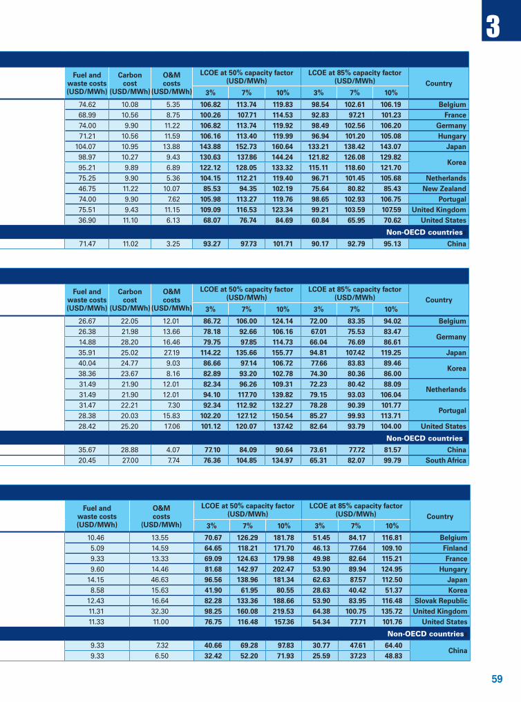
59

3

59

Table 3.16: Levelised cost of electricity for combined-cycle gas turbines, 50% and 85% capacity factor

Country TechnologyInvestment cost1

(USD/MWh)Refurbishment and decom­

missioning costs (USD/MWh)Fuel and

waste costs (USD/MWh)

Carbon cost

(USD/MWh)

O&M costs

(USD/MWh)

LCOE at 50% capacity factor (USD/MWh)

LCOE at 85% capacity factor (USD/MWh) Country

3% 7% 10% 3% 7% 10% 3% 7% 10% 3% 7% 10%

Belgium CCGT 16.41 23.49 29.66 0.36 0.20 0.12 74.62 10.08 5.35 106.82 113.74 119.83 98.54 102.61 106.19 BelgiumFrance CCGT 11.76 19.32 26.19 0.19 0.08 0.04 68.99 10.56 8.75 100.26 107.71 114.53 92.83 97.21 101.23 FranceGermany CCGT 11.51 18.54 24.76 0.19 0.08 0.04 74.00 9.90 11.22 106.82 113.74 119.92 98.49 102.56 106.20 GermanyHungary CCGT (dual fuel) 12.81 20.04 26.63 0.00 0.00 0.00 71.21 10.56 11.59 106.16 113.40 119.99 96.94 101.20 105.08 HungaryJapan CCGT 14.74 23.73 31.70 0.26 0.11 0.05 104.07 10.95 13.88 143.88 152.73 160.64 133.21 138.42 143.07 Japan

KoreaCCGT 11.96 19.19 25.56 0.00 0.00 0.00 98.97 10.27 9.43 130.63 137.86 144.24 121.82 126.08 129.82

KoreaCCGT 9.96 15.98 21.29 0.17 0.07 0.04 95.21 9.89 6.89 122.12 128.05 133.32 115.11 118.60 121.70

Netherlands CCGT 13.41 21.60 28.84 0.22 0.09 0.05 75.25 9.90 5.36 104.15 112.21 119.40 96.71 101.45 105.68 NetherlandsNew Zealand CCGT 17.16 26.14 34.05 0.33 0.16 0.09 46.75 11.22 10.07 85.53 94.35 102.19 75.64 80.82 85.43 New ZealandPortugal CCGT 14.20 21.63 28.17 0.27 0.13 0.07 74.00 9.90 7.62 105.98 113.27 119.76 98.65 102.93 106.75 PortugalUnited Kingdom CCGT 12.99 20.43 27.24 0.00 0.00 0.00 75.51 9.43 11.15 109.09 116.53 123.34 99.21 103.59 107.59 United KingdomUnited States CCGT 13.71 22.52 30.51 0.22 0.09 0.05 36.90 11.10 6.13 68.07 76.74 84.69 60.84 65.95 70.62 United States

Non-OECD countries Non-OECD countriess

China CCGT 7.42 11.94 15.95 0.12 0.05 0.03 71.47 11.02 3.25 93.27 97.73 101.71 90.17 92.79 95.13 China

1. Investment cost includes overnight cost (with contingency) as well as the implied IDC.

Table 3.17: Levelised cost of electricity for coal technologies, 50% and 85% capacity factor

Country TechnologyInvestment cost1

(USD/MWh)Refurbishment and decom­

missioning costs (USD/MWh)Fuel and

waste costs (USD/MWh)

Carbon cost

(USD/MWh)

O&M costs

(USD/MWh)

LCOE at 50% capacity factor (USD/MWh)

LCOE at 85% capacity factor (USD/MWh) Country

3% 7% 10% 3% 7% 10% 3% 7% 10% 3% 7% 10%

Belgium Ultra-supercritical 25.63 45.15 63.36 0.35 0.13 0.06 26.67 22.05 12.01 86.72 106.00 124.14 72.00 83.35 94.02 Belgium

GermanyHard coal 16.00 30.60 44.13 0.16 0.04 0.02 26.38 21.98 13.66 78.18 92.66 106.16 67.01 75.53 83.47

GermanyLignite 20.00 38.25 55.16 0.20 0.05 0.02 14.88 28.20 16.46 79.75 97.85 114.73 66.04 76.69 86.61

Japan Ultra-supercritical 25.78 47.44 67.61 0.32 0.10 0.04 35.91 25.02 27.19 114.22 135.66 155.77 94.81 107.42 119.25 Japan

KoreaPulverised (PC 800) 12.82 23.30 32.88 0.00 0.00 0.00 40.04 24.77 9.03 86.66 97.14 106.72 77.66 83.83 89.46

KoreaPulverised (PC 1000) 12.54 22.95 32.57 0.15 0.05 0.02 38.36 23.67 8.16 82.89 93.20 102.78 74.30 80.36 86.00

NetherlandsUltra-supercritical 16.74 30.79 43.88 0.20 0.06 0.02 31.49 21.90 12.01 82.34 96.26 109.31 72.23 80.42 88.09

NetherlandsUltra-supercritical 28.36 52.19 74.37 0.34 0.10 0.04 31.49 21.90 12.01 94.10 117.70 139.82 79.15 93.03 106.04

PortugalPulverised 30.86 51.74 71.19 0.49 0.20 0.10 31.47 22.21 7.30 92.34 112.92 132.27 78.28 90.39 101.77

PortugalPulverised 37.36 62.63 86.17 0.60 0.25 0.12 28.38 20.03 15.83 102.20 127.12 150.54 85.27 99.93 113.71

United States Supercritical pulverised 29.95 49.18 66.64 0.49 0.20 0.10 28.42 25.20 17.06 101.12 120.07 137.42 82.64 93.79 104.00 United States

Non-OECD countries Non-OECD countriess

China Ultra-supercritical 8.40 15.45 22.02 0.10 0.03 0.01 35.67 28.88 4.07 77.10 84.09 90.64 73.61 77.72 81.57 ChinaSouth Africa Pulverised 21.04 49.63 79.77 0.12 0.02 0.00 20.45 27.00 7.74 76.36 104.85 134.97 65.31 82.07 99.79 South Africa

1. Investment cost includes overnight cost (with contingency) as well as the implied IDC.

Table 3.18: Levelised cost of electricity for nuclear technologies, 50% and 85% capacity factor

Country TechnologyInvestment cost1

(USD/MWh)Refurbishment and decom­

missioning costs (USD/MWh)Fuel and

waste costs (USD/MWh)

O&M costs

(USD/MWh)

LCOE at 50% capacity factor (USD/MWh)

LCOE at 85% capacity factor (USD/MWh) Country

3% 7% 10% 3% 7% 10% 3% 7% 10% 3% 7% 10%

Belgium Gen III projects 45.88 102.15 157.74 0.77 0.13 0.03 10.46 13.55 70.67 126.29 181.78 51.45 84.17 116.81 BelgiumFinland ALWR 44.21 98.43 152.00 0.75 0.10 0.02 5.09 14.59 64.65 118.21 171.70 46.13 77.64 109.10 FinlandFrance ALWR 45.75 101.87 157.30 0.67 0.10 0.02 9.33 13.33 69.09 124.63 179.98 49.98 82.64 115.21 FranceHungary ALWR 54.92 118.46 178.31 2.71 0.45 0.10 9.60 14.46 81.68 142.97 202.47 53.90 89.94 124.95 HungaryJapan Advanced LWR 35.06 78.06 120.53 0.72 0.12 0.03 14.15 46.63 96.56 138.96 181.34 62.63 87.57 112.50 JapanKorea ALWR 17.70 37.74 56.35 0.00 0.00 0.00 8.58 15.63 41.90 61.95 80.55 28.63 40.42 51.37 KoreaSlovak Republic LWR 45.30 101.74 158.19 7.91 2.55 1.41 12.43 16.64 82.28 133.36 188.66 53.90 83.95 116.48 Slovak RepublicUnited Kingdom ALWR 53.71 116.32 175.88 0.92 0.15 0.04 11.31 32.30 98.25 160.08 219.53 64.38 100.75 135.72 United KingdomUnited States ALWR 52.28 93.26 134.58 2.14 0.89 0.45 11.33 11.00 76.75 116.48 157.36 54.34 77.71 101.76 United States

Non-OECD countries Non-OECD countriess

ChinaALWR 23.61 52.57 81.17 0.40 0.07 0.02 9.33 7.32 40.66 69.28 97.83 30.77 47.61 64.40

ChinaALWR 16.31 36.32 56.09 0.28 0.05 0.01 9.33 6.50 32.42 52.20 71.93 25.59 37.23 48.83

1. Investment cost includes overnight cost (with contingency) as well as the implied IDC.

60

3

60

When comparing the LCOEs at 85% and 50% capacity factors, it is immediately clear that nuclear technologies are far more sensitive to changes in capacity factor than natural gas and coal technologies. Focusing on the LCOEs at a discount rate of 7%, the cost of natural gas-fired generation increases by 11% on average, and coal-fired generation by an average of 23%. The cost for the nuclear generators increases by 54% on average.

In practice this means that, on average, nuclear generation goes from being the least expensive baseload technology on a levelised basis (USD 76/MWh at a 7% discount rate and 85% capacity factor) to the most expensive (USD  117/MWh). Natural gas generation increases from USD  102/MWh on average, to USD 114/MWh, while coal generation increases from USD 87 to USD 107/MWh. While coal is still relatively cheaper than natural gas on average, the gap in cost is significantly diminished. At a 10% discount rate, natural gas becomes the least expensive technology at USD 120/MWh, compared to USD 123/MWh for coal and USD 164/MWh for nuclear.

The impact of capacity factor on the cost of the specific plants in the EGC database is also explored on a country-by-country basis in Section 4.2.

References

Fraunhofer-Institut für Solare Energiesysteme ISE (2013), Stromgestehungskosten Erneuerbare Energien, Freiburg, www.ise.fraunhofer.de/de/veroeffentlichungen/veroeffentlichungen-pdf-dateien/studien-und-konzeptpapiere/studie-stromgestehungskosten-erneuerbare-energien.pdf.

IEA (2014), World Energy Investment Outlook 2014, OECD, Paris.

NEA (2012), Economics of the Back End of the Nuclear Fuel Cycle, OECD, Paris, www.oecd-nea.org/ndd/pubs/2013/7061-ebenfc.pdf.

Prognos (2013), Entwicklung von Stromproduktionskosten, Berlin, www.prognos.com/fileadmin/pdf/aktuelles/131010_Studie_Belectric_Freiflaechen_Solarkraftwerke_Final.pdf.

Prognos et al. (2014), Entwicklung der Energiemärkte – Energiereferenzprognose, Berlin, pp. 71 and pp.  466-467 www.bmwi.de/BMWi/Redaktion/PDF/Publikationen/entwicklung-der-energiemaerkte-energiereferenzprognose-endbericht,property=pdf,bereich=bmwi2012,sprache=de,rwb=true.pdf.

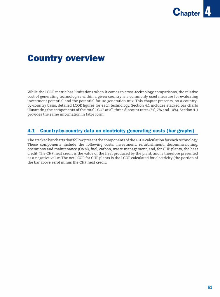
61

4

61

Chapter

Country overview

While the LCOE metric has limitations when it comes to cross-technology comparisons, the relative cost of generating technologies within a given country is a commonly used measure for evaluating investment potential and the potential future generation mix. This chapter presents, on a country-by-country basis, detailed LCOE figures for each technology. Section 4.1 includes stacked bar charts illustrating the components of the total LCOE at all three discount rates (3%, 7% and 10%). Section 4.3 provides the same information in table form.

4.1 Country-by-country data on electricity generating costs (bar graphs)

The stacked bar charts that follow present the components of the LCOE calculation for each technology. These components include the following costs: investment, refurbishment, decommissioning, operations and maintenance (O&M), fuel, carbon, waste management, and, for CHP plants, the heat credit. The CHP heat credit is the value of the heat produced by the plant, and is therefore presented as a negative value. The net LCOE for CHP plants is the LCOE calculated for electricity (the portion of the bar above zero) minus the CHP heat credit.

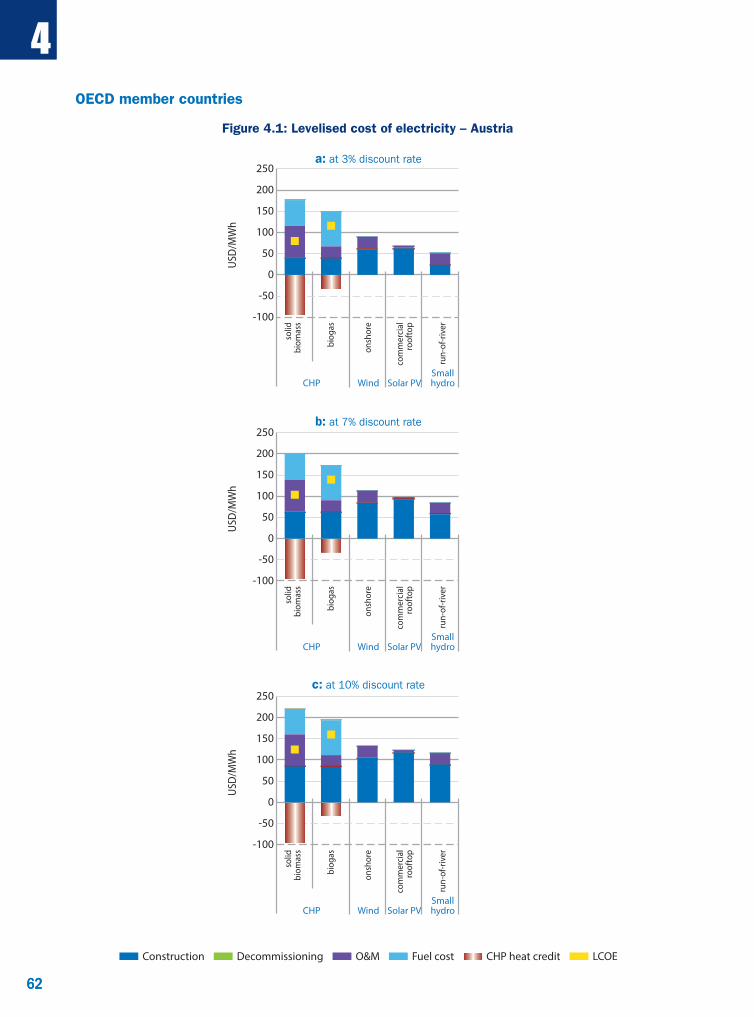
62

4

62

Figure 4.1: Levelised cost of electricity – Austria

USD

/MW

h

c: at 10% discount rate

Solar PVWindCHPSmallhydro

solid

bi

omas

s

biog

as

onsh

ore

com

mer

cial

ro

ofto

p

run-

of-r

iver

b: at 7% discount rate

a: at 3% discount rate

-100

-50

0

50

100

150

200

250

USD

/MW

h

Solar PVWindCHPSmallhydro

solid

bi

omas

s

biog

as

onsh

ore

com

mer

cial

ro

ofto

p

run-

of-r

iver

-100

-50

0

50

100

150

200

250

USD

/MW

h

Solar PVWindCHPSmallhydro

solid

bi

omas

s

biog

as

onsh

ore

com

mer

cial

ro

ofto

p

run-

of-r

iver

-100

-50

0

50

100

150

200

250

DecommissioningConstruction O&M Fuel cost CHP heat credit LCOE

OECD member countries

63

4

63

Figure 4.2: Levelised cost of electricity – Belgium

USD

/MW

h

ultr

a-su

perc

ritic

al

resid

entia

l ro

ofto

p

com

mer

cial

ro

ofto

p

Solar PVWindNuclearCoalOCGTCCGT

DecommissioningConstruction Carbon costO&M Fuel cost Waste management

a: at 3% discount rate

0

50

100

150

200

250

300

350

onshore o�shore

USD

/MW

h

ultr

a-su

perc

ritic

al

resid

entia

l ro

ofto

p

com

mer

cial

ro

ofto

p

Solar PVWindNuclearCoalOCGTCCGT

b: at 7% discount rate

0

50

100

150

200

250

300

350

onshore o�shore

USD

/MW

h

ultr

a-su

perc

ritic

al

resid

entia

l ro

ofto

p

com

mer

cial

ro

ofto

p

Solar PVWindNuclearCoalOCGTCCGT

c: at 10% discount rate

0

50

100

150

200

250

300

350

onshore o�shore

64

4

64

Figure 4.3: Levelised cost of electricity – Denmark

USD

/MW

h

c: at 10% discount rate

CHP medium CHP large Wind Solar PV

woo

d ch

ips

stra

w

natu

ral g

as

woo

d pe

llets

coal

natu

ral g

as

onsh

ore

o�sh

ore

resid

entia

l roo

ftop

com

mer

cial

roof

top

larg

e, g

roun

d-m

ount

ed

b: at 7% discount rate

a: at 3% discount rate

DecommissioningConstruction Carbon costO&M Fuel costCHP heat credit LCOE

-100-50

050

100150200250300350

USD

/MW

h

CHP medium CHP large Wind Solar PV

woo

d ch

ips

stra

w

natu

ral g

as

woo

d pe

llets

coal

natu

ral g

as

onsh

ore

o�sh

ore

resid

entia

l roo

ftop

com

mer

cial

roof

top

larg

e, g

roun

d-m

ount

ed-100

-500

50100150200250300350

USD

/MW

h

CHP medium CHP large Wind Solar PV

woo

d ch

ips

stra

w

natu

ral g

as

woo

d pe

llets

coal

natu

ral g

as

onsh

ore

o�sh

ore

resid

entia

l roo

ftop

com

mer

cial

roof

top

larg

e, g

roun

d-m

ount

ed

-100-50

050

100150200250300350

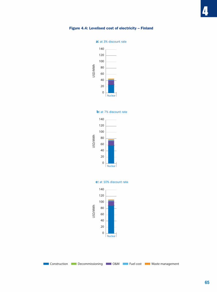
65

4

65

Figure 4.4: Levelised cost of electricity – Finland

USD

/MW

h

DecommissioningConstruction O&M Fuel cost Waste management

a: at 3% discount rate

Nuclear

b: at 7% discount rate

c: at 10% discount rate

0

20

40

60

80

100

120

140

USD

/MW

h

Nuclear0

20

40

60

80

100

120

140

USD

/MW

h

Nuclear0

20

40

60

80

100

120

140

66

4

66

Figure 4.5: Levelised cost of electricity – France

USD

/MW

h

resid

entia

l ro

ofto

p

com

mer

cial

ro

ofto

p

larg

e, g

roun

d-m

ount

ed

Solar PVWindNuclearCCGT

DecommissioningConstruction Carbon costO&M Fuel cost Waste management

a: at 3% discount rate

onshore o�shore0

50

100

150

200

250

300

350

400

USD

/MW

h

resid

entia

l ro

ofto

p

com

mer

cial

ro

ofto

p

larg

e, g

roun

d-m

ount

ed

Solar PVWindNuclearCCGT

b: at 7% discount rate

onshore o�shore0

50

100

150

200

250

300

350

400

USD

/MW

h

resid

entia

l ro

ofto

p

com

mer

cial

ro

ofto

p

larg

e, g

roun

d-m

ount

ed

Solar PVWindNuclearCCGT

c: at 10% discount rate

onshore o�shore0

50

100

150

200

250

300

350

400

67

4

67

Figure 4.6: Levelised cost of electricity – Germany

b: at 7% discount rate

a: at 3% discount rate

DecommissioningRefurbishmentConstruction Carbon costO&M Fuel costCHP heat credit LCOE

Coal CHP Wind

USD

/MW

h

hard

coa

l

ligni

te

engi

ne –

bi

ogas

(dig

este

r)

engi

ne –

biog

as

engi

ne –

min

e ga

s

stea

m tu

rbin

e –

solid

bio

mas

s

geot

herm

al

onsh

ore

o�sh

ore

resid

entia

l ro

ofto

p

com

mer

cial

roof

top

larg

e, g

roun

d-m

ount

ed

smal

l –ru

n-of

-riv

er

larg

e –

run-

of-r

iver

CCGT OCGT Solar PV

c: at 10% discount rate

-200

-100

0

100

200

300

400

500

Coal CHP Wind Hydro

Hydro

Hydro

USD

/MW

h

hard

coa

l

ligni

te

engi

ne –

bi

ogas

(dig

este

r)

engi

ne –

biog

as

engi

ne –

min

e ga

s

stea

m tu

rbin

e –

solid

bio

mas

s

geot

herm

al

onsh

ore

o�sh

ore

resid

entia

l ro

ofto

p

com

mer

cial

roof

top

larg

e, g

roun

d-m

ount

ed

smal

l –ru

n-of

-riv

er

larg

e –

run-

of-r

iver

CCGT OCGT Solar PV

-200

-100

0

100

200

300

400

500

Coal CHP Wind

USD

/MW

h

hard

coa

l

ligni

te

engi

ne –

bi

ogas

(dig

este

r)

engi

ne –

biog

as

engi

ne –

min

e ga

s

stea

m tu

rbin

e –

solid

bio

mas

s

geot

herm

al

onsh

ore

o�sh

ore

resid

entia

l ro

ofto

p

com

mer

cial

roof

top

larg

e, g

roun

d-m

ount

ed

smal

l –ru

n-of

-riv

er

larg

e –

run-

of-r

iver

CCGT OCGT Solar PV

-200

-100

0

100

200

300

400

500

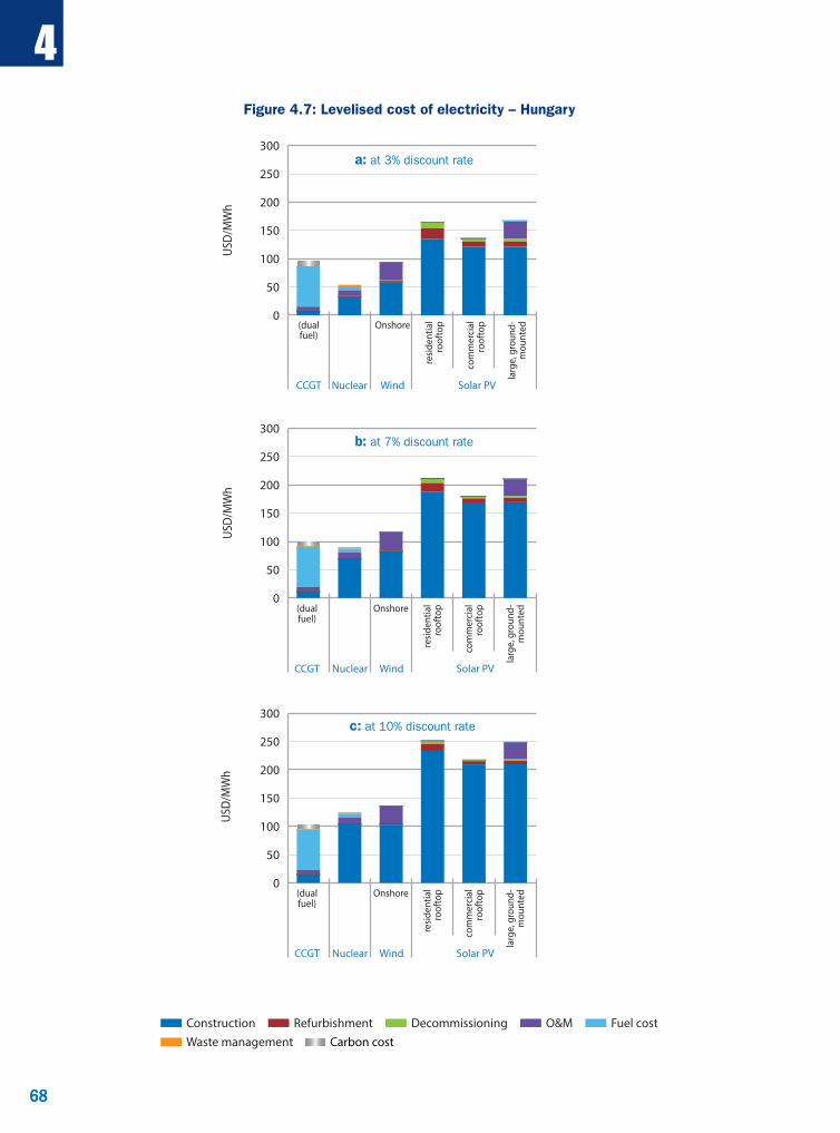
68

4

68

Figure 4.7: Levelised cost of electricity – Hungary

USD

/MW

h

DecommissioningRefurbishmentConstructionCarbon cost

O&M Fuel costWaste management

c: at 10% discount rate

0

50

100

150

200

250

300

resid

entia

l ro

ofto

p

com

mer

cial

ro

ofto

p

larg

e, g

roun

d-m

ount

ed

Solar PVWindNuclearCCGT

(dualfuel)

Onshore

resid

entia

l ro

ofto

p

com

mer

cial

ro

ofto

p

larg

e, g

roun

d-m

ount

ed

Solar PVWindNuclearCCGT

(dualfuel)

Onshore

USD

/MW

hUS

D/M

Wh

a: at 3% discount rate

b: at 7% discount rate

0

50

100

150

200

250

300

0

50

100

150

200

250

300

resid

entia

l ro

ofto

p

com

mer

cial

ro

ofto

p

larg

e, g

roun

d-m

ount

ed

Solar PVWindNuclearCCGT

(dualfuel)

Onshore

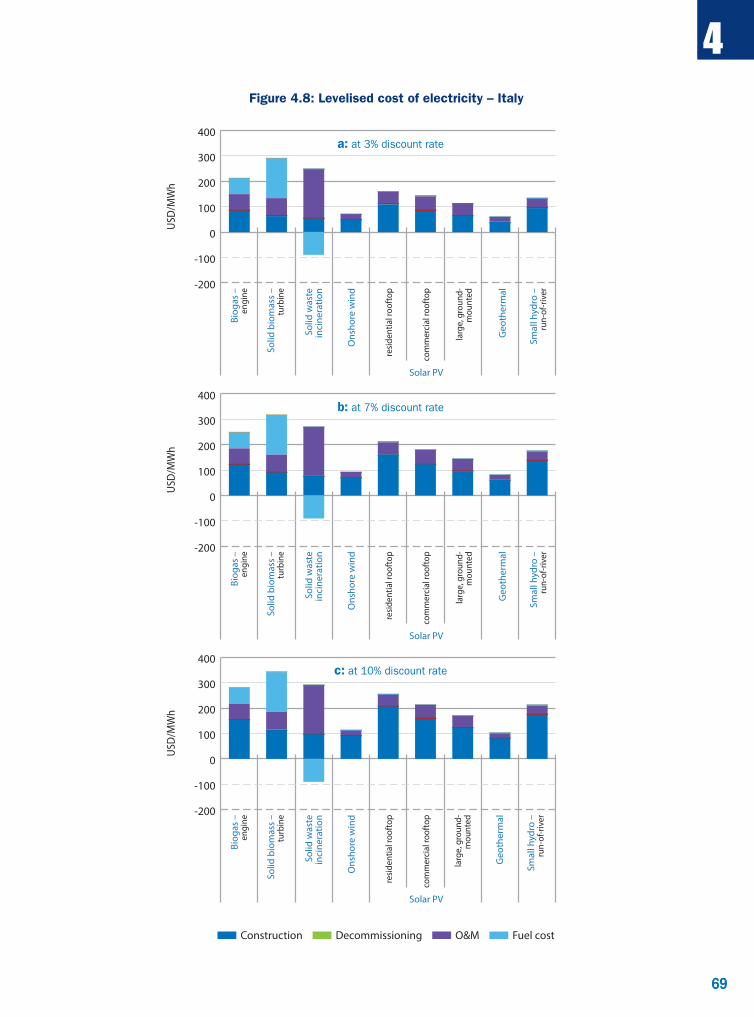
69

4

69

Figure 4.8: Levelised cost of electricity – Italy

DecommissioningConstruction O&M Fuel cost

USD

/MW

h

c: at 10% discount rate

-200

-100

0

100

200

300

400

Solar PV

Biog

as –

en

gine

Solid

bio

mas

s –

turb

ine

Solid

was

tein

cine

ratio

n

Ons

hore

win

d

resid

entia

l roo

ftop

com

mer

cial

roof

top

larg

e, g

roun

d-m

ount

ed

Geo

ther

mal

Smal

l hyd

ro –

ru

n-of

-riv

er

USD

/MW

h

b: at 7% discount rate

-200

-100

0

100

200

300

400

Solar PV

Biog

as –

en

gine

Solid

bio

mas

s –

turb

ine

Solid

was

tein

cine

ratio

n

Ons

hore

win

d

resid

entia

l roo

ftop

com

mer

cial

roof

top

larg

e, g

roun

d-m

ount

ed

Geo

ther

mal

Smal

l hyd

ro –

ru

n-of

-riv

er

USD

/MW

h

a: at 3% discount rate

-200

-100

0

100

200

300

400

Solar PV

Biog

as –

en

gine

Solid

bio

mas

s –

turb

ine

Solid

was

tein

cine

ratio

n

Ons

hore

win

d

resid

entia

l roo

ftop

com

mer

cial

roof

top

larg

e, g

roun

d-m

ount

ed

Geo

ther

mal

Smal

l hyd

ro –

ru

n-of

-riv

er

70

4

70

Figure 4.9: Levelised cost of electricity – Japan

USD

/MW

h

resid

entia

l ro

ofto

p

larg

e, g

roun

d-m

ount

ed

Solar PVLarge hydroWindCoal NuclearCCGT

DecommissioningConstruction Carbon costO&M Fuel cost Waste management

a: at 3% discount rate

onshore

ultr

a-su

perc

ritic

al0

50

100

150

200

250

300

350

400

USD

/MW

h

resid

entia

l ro

ofto

p

larg

e, g

roun

d-m

ount

ed

Solar PVLarge hydroWindCoal NuclearCCGT

b: at 7% discount rate

onshore

ultr

a-su

perc

ritic

al

0

50

100

150

200

250

300

350

400

USD

/MW

h

resid

entia

l ro

ofto

p

larg

e, g

roun

d-m

ount

ed

Solar PVLarge hydroWindCoal NuclearCCGT

c: at 10% discount rate

onshore

ultr

a-su

perc

ritic

al

0

50

100

150

200

250

300

350

400

71

4

71

Figure 4.10: Levelised cost of electricity – Korea

DecommissioningConstruction Carbon costO&M Fuel cost Waste management

USD

/MW

h

pul

veris

ed(P

C 10

00)

pulv

erise

d(P

C 80

0)

resid

entia

l ro

ofto

p

com

mer

cial

ro

ofto

p

larg

e, g

rond

-m

ount

ed

c: at 10% discount rate

0

50

100

150

200

250

300

350

Solar PVWindNuclearCoalCCGTCCGT

onshore o�shore

USD

/MW

h

pul

veris

ed(P

C 10

00)

pulv

erise

d(P

C 80

0)

resid

entia

l ro

ofto

p

com

mer

cial

ro

ofto

p

larg

e, g

rond

-m

ount

ed

b: at 7% discount rate

0

50

100

150

200

250

300

350

Solar PVWindNuclearCoalCCGTCCGT

onshore o�shore

USD

/MW

h

pul

veris

ed(P

C 10

00)

pulv

erise

d(P

C 80

0)

resid

entia

l ro

ofto

p

com

mer

cial

ro

ofto

p

larg

e, g

rond

-m

ount

ed

a: at 3% discount rate

0

50

100

150

200

250

300

350

Solar PVWindNuclearCoalCCGTCCGT

onshore o�shore

72

4

72

Figure 4.11: Levelised cost of electricity – Netherlands US

D/M

Wh

c: at 10% discount rate

CCGT Coal CHP

Solidwasteincin-

erationCo-

�ring Wind Solar PV

woo

d pe

llets

onsh

ore

o�sh

ore

com

mer

cial

ro

ofto

p

b: at 7% discount rate

a: at 3% discount rate

DecommissioningRefurbishmentConstruction Carbon costO&M Fuel costCHP heat credit LCOE

-50

0

50

100

150

200

250

ultra-supercritical fermentation

USD

/MW

h

CCGT Coal CHP

Solidwasteincin-

erationCo-

�ring Wind Solar PV

woo

d pe

llets

onsh

ore

o�sh

ore

com

mer

cial

ro

ofto

p-50

0

50

100

150

200

250

ultra-supercritical fermentation

USD

/MW

h

CCGT Coal CHP

Solidwasteincin-

erationCo-

�ring Wind Solar PV

woo

d pe

llets

onsh

ore

o�sh

ore

com

mer

cial

ro

ofto

p-50

0

50

100

150

200

250

ultra-supercritical fermentation

73

4

73

Figure 4.12: Levelised cost of electricity – New Zealand

DecommissioningConstruction Carbon costO&M Fuel cost

USD

/MW

h

c: at 10% discount rate

020406080

100120140160180

OCGTGeo-

thermalCCGT

USD

/MW

h

b: at 7% discount rate

020406080

100120140160180

OCGTGeo-

thermalCCGT

USD

/MW

h

a: at 3% discount rate

020406080

100120140160180

OCGT WindGeo-

thermalCCGT

onshore

Wind

onshore

Wind

onshore

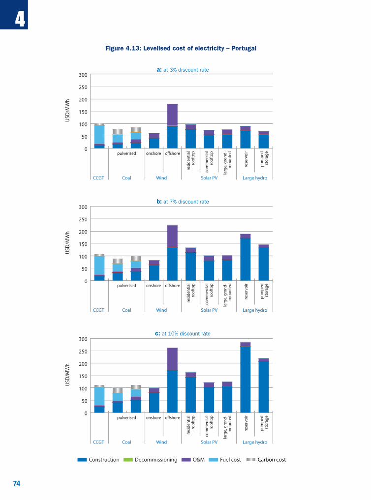
74

4

74

Figure 4.13: Levelised cost of electricity – Portugal

DecommissioningConstruction Carbon costO&M Fuel cost

c: at 10% discount rate

b: at 7% discount rate

USD

/MW

h

resid

entia

l ro

ofto

p

com

mer

cial

ro

ofto

p

larg

e, g

rond

-m

ount

ed

rese

rvoi

r

pum

ped

stor

age

a: at 3% discount rate

Solar PV Large hydroWindCoalCCGT

pulverised o�shoreonshore0

50

100

150

200

250

300US

D/M

Wh

resid

entia

l ro

ofto

p

com

mer

cial

ro

ofto

p

larg

e, g

rond

-m

ount

ed

rese

rvoi

r

pum

ped

stor

age

Solar PV Large hydroWindCoalCCGT

pulverised o�shoreonshore0

50

100

150

200

250

300

USD

/MW

h

resid

entia

l ro

ofto

p

com

mer

cial

ro

ofto

p

larg

e, g

rond

-m

ount

ed

rese

rvoi

r

pum

ped

stor

age

Solar PV Large hydroWindCoalCCGT

pulverised o�shoreonshore0

50

100

150

200

250

300

75

4

75

Figure 4.14: Levelised cost of electricity – Slovak Republic

USD

/MW

h

DecommissioningConstruction Refurbishment O&M Fuel cost Waste management

a: at 3% discount rate

Nuclear

b: at 7% discount rate

c: at 10% discount rate

0

20

40

60

80

100

120

USD

/MW

h

Nuclear0

20

40

60

80

100

120

USD

/MW

h

Nuclear0

20

40

60

80

100

120

76

4

76

Figure 4.15: Levelised cost of electricity – Spain

b: at 7% discount rate

a: at 3% discount rate

DecommissioningConstruction Carbon costO&M Fuel costCHP heat credit LCOE

CHP Wind

USD

/MW

h

turb

ine

turb

ine

engi

ne

gas t

urbi

ne

onsh

ore

resid

entia

l ro

ofto

p

com

mer

cial

roof

top

larg

e, g

roun

d-m

ount

ed

ther

mal

(CSP

) –no

stor

age

smal

l –ru

n-of

-riv

er

larg

e –

run-

of-r

iver

smal

l –re

serv

oir

larg

e –

rese

rvoi

r

Bio-mass Biogas Solar PV Solar

c: at 10% discount rate

Hydro

-200

-100

0

100

200

300

400

500

engine

CHP Wind

USD

/MW

h

turb

ine

turb

ine

engi

ne

gas t

urbi

ne

onsh

ore

resid

entia

l ro

ofto

p

com

mer

cial

roof

top

larg

e, g

roun

d-m

ount

ed

ther

mal

(CSP

) –no

stor

age

smal

l –ru

n-of

-riv

er

larg

e –

run-

of-r

iver

smal

l –re

serv

oir

larg

e –

rese

rvoi

r

Bio-mass Biogas Solar PV Solar Hydro

-200

-100

0

100

200

300

400

500

engine

CHP Wind

USD

/MW

h

turb

ine

turb

ine

engi

ne

gas t

urbi

ne

onsh

ore

resid

entia

l ro

ofto

p

com

mer

cial

roof

top

larg

e, g

roun

d-m

ount

ed

ther

mal

(CSP

) –no

stor

age

smal

l –ru

n-of

-riv

er

larg

e –

run-

of-r

iver

smal

l –re

serv

oir

larg

e –

rese

rvoi

r

Bio-mass Biogas Solar PV Solar Hydro

-200

-100

0

100

200

300

400

500

engine

Solidwasteincin-

eration

Solidwasteincin-

eration

Solidwasteincin-

eration

77

4

77

Figure 4.16: Levelised cost of electricity – Switzerland

DecommissioningConstruction O&M

USD

/MW

h

c: at 10% discount rate

0

50

100

150

200

250

300

350

400

Solar PVSmallhydro

Largehydro

com

mer

cial

ro

ofto

p

run-

of-r

iver

run-

of-r

iver

rese

rvoi

r

pum

ped

stor

age

USD

/MW

h

b: at 7% discount rate

0

50

100

150

200

250

300

350

400

Solar PVSmallhydro

Largehydro

com

mer

cial

ro

ofto

p

run-

of-r

iver

run-

of-r

iver

rese

rvoi

r

pum

ped

stor

age

USD

/MW

h

a: at 3% discount rate

0

50

100

150

200

250

300

350

400

Solar PVSmallhydro

Largehydro

com

mer

cial

ro

ofto

p

run-

of-r

iver

run-

of-r

iver

rese

rvoi

r

pum

ped

stor

age

78

4

78

Figure 4.17: Levelised cost of electricity – Turkey

RefurbishmentConstruction Decommissioning

USD

/MW

h

c: at 10% discount rate

b: at 7% discount rate

Geo-thermal

Largehydro

a: at 3% discount rate

Wind

0

20

40

60

80

100

120

140

onshore reservoir

USD

/MW

h

Geo-thermal

LargehydroWind

0

20

40

60

80

100

120

140

onshore reservoir

USD

/MW

h

Geo-thermal

LargehydroWind

0

20

40

60

80

100

120

140

onshore reservoir

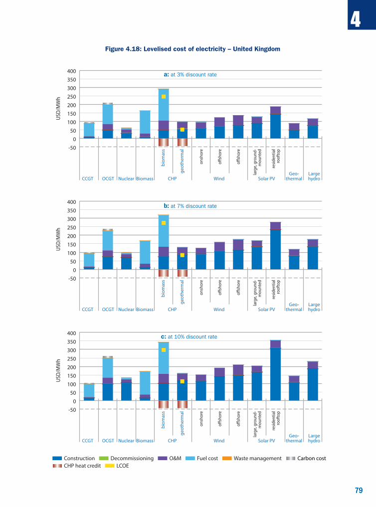
79

4

79

Figure 4.18: Levelised cost of electricity – United Kingdom

c: at 10% discount rate

CCGT OCGT Nuclear Biomass CHP Wind Solar PVGeo-

thermalLargehydro

onsh

ore

o�sh

ore

o�sh

ore

larg

e, g

roun

d-m

ount

ed

resid

entia

l ro

ofto

p

biom

ass

geot

herm

al

b: at 7% discount rate

a: at 3% discount rate

DecommissioningConstruction Carbon costO&M Fuel cost Waste managementCHP heat credit LCOE

USD

/MW

h

-500

50100150200250300350400

CCGT OCGT Nuclear Biomass CHP Wind Solar PVGeo-

thermalLargehydro

onsh

ore

o�sh

ore

o�sh

ore

larg

e, g

roun

d-m

ount

ed

resid

entia

l ro

ofto

p

biom

ass

geot

herm

al

USD

/MW

h

-500

50100150200250300350400

CCGT OCGT Nuclear Biomass CHP Wind Solar PVGeo-

thermalLargehydro

onsh

ore

o�sh

ore

o�sh

ore

larg

e, g

roun

d-m

ount

ed

resid

entia

l ro

ofto

p

biom

ass

geot

herm

al

USD

/MW

h

-500

50100150200250300350400

80

4

80

Figure 4.19: Levelised cost of electricity – United States – Nuclear, fossil and biomass technologies

USD

/MW

h

c: at 10% discount rate

Coal BiomassCCGT

b: at 7% discount rate

a: at 3% discount rate

Nuclear

supe

rcrit

ical

pulv

erise

d

0

20

40

60

80

100

120

140

USD

/MW

h

Coal BiomassCCGT Nuclear

supe

rcrit

ical

pulv

erise

d

0

20

40

60

80

100

120

140

USD

/MW

h

Coal BiomassCCGT Nuclear

supe

rcrit

ical

pulv

erise

d

0

20

40

60

80

100

120

140

DecommissioningConstruction Carbon costO&M Fuel cost Waste management

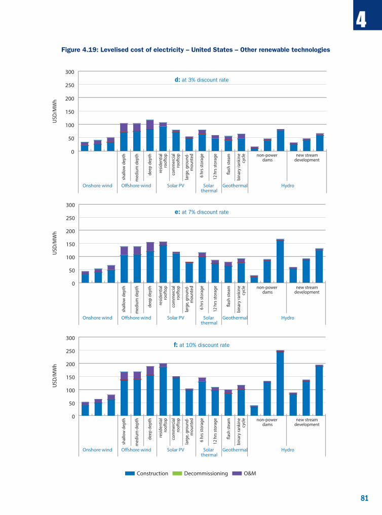
81

4

81

Figure 4.19: Levelised cost of electricity – United States – Other renewable technologies US

D/M

Wh

USD

/MW

h

shal

low

dep

th

med

ium

dep

th

deep

dep

th

resid

entia

l ro

ofto

p

com

mer

cial

roof

top

larg

e, g

roun

d-m

ount

ed

6 hr

s sto

rage

12 h

rs st

orag

e

�ash

stea

m

bina

ry ra

nkin

ecy

cle

Onshore wind

non-power dams

new streamdevelopment

O�shore wind Solar PV Solar thermal

Geothermal Hydro

shal

low

dep

th

med

ium

dep

th

deep

dep

th

resid

entia

l ro

ofto

p

com

mer

cial

roof

top

larg

e, g

roun

d-m

ount

ed

6 hr

s sto

rage

12 h

rs st

orag

e

�ash

stea

m

bina

ry ra

nkin

ecy

cle

Onshore wind

non-power dams

new streamdevelopment

O�shore wind Solar PV Solar thermal

Geothermal Hydro

DecommissioningConstruction O&M

d: at 3% discount rate

0

50

100

150

200

250

300

USD

/MW

h

shal

low

dep

th

med

ium

dep

th

deep

dep

th

resid

entia

l ro

ofto

p

com

mer

cial

roof

top

larg

e, g

roun

d-m

ount

ed

6 hr

s sto

rage

12 h

rs st

orag

e

�ash

stea

m

bina

ry ra

nkin

ecy

cle

Onshore wind

non-power dams

new streamdevelopment

O�shore wind Solar PV Solar thermal

Geothermal Hydro

e: at 7% discount rate

f: at 10% discount rate

0

50

100

150

200

250

300

0

50

100

150

200

250

300

82

4

82

Figure 4.20: Levelised cost of electricity – Brazil

USD

/MW

h

c: at 10% discount rate

Large hydro

b: at 7% discount rate

a: at 3% discount rate

DecommissioningConstruction O&M

0

20

40

60

80

100

120

run-of-river

USD

/MW

h

Large hydro

0

20

40

60

80

100

120

run-of-river

USD

/MW

h

Large hydro

0

20

40

60

80

100

120

run-of-river

Non-OECD countries

83

4

83

Figure 4.21: Levelised cost of electricity – China

c: at 10% discount rate

b: at 7% discount rate

com

mer

cial

ro

ofto

p

larg

e, g

rond

-m

ount

ed

rese

rvoi

r

a: at 3% discount rate

Solar PVWindLarge hydro

Solar PVLarge hydro

Solar PVLarge hydro

CoalCCGT

ultr

a-su

perc

ritic

al onshore onshore

USD

/MW

h

0

20

40

60

80

100

com

mer

cial

ro

ofto

p

larg

e, g

rond

-m

ount

ed

rese

rvoi

r

WindCoalCCGT

ultr

a-su

perc

ritic

al onshore onshore

USD

/MW

h

0

20

40

60

80

100co

mm

erci

al

roof

top

larg

e, g

rond

-m

ount

ed

rese

rvoi

r

WindNuclear 1 Nuclear 2

Nuclear 1 Nuclear 2

Nuclear 1 Nuclear 2

CoalCCGT

ultr

a-su

perc

ritic

al onshore onshore

USD

/MW

h

0

20

40

60

80

100

DecommissioningConstruction Carbon costO&M Fuel cost Waste management

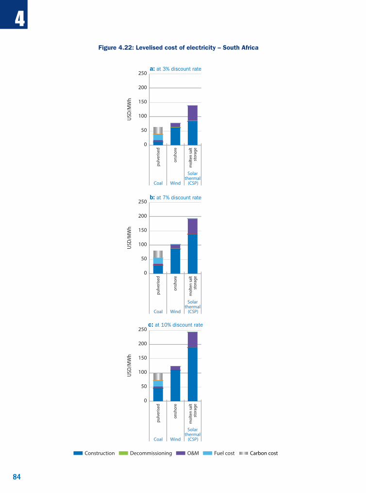
84

4

84

Figure 4.22: Levelised cost of electricity – South Africa

USD

/MW

h

c: at 10% discount rate

b: at 7% discount rate

Solar thermal

(CSP)

a: at 3% discount rate

Wind

onsh

ore

Coal

pulv

erise

d

mol

ten

salt

stor

age

0

50

100

150

200

250

USD

/MW

h

Solar thermal

(CSP)Wind

onsh

ore

Coal

pulv

erise

d

mol

ten

salt

stor

age

0

50

100

150

200

250

USD

/MW

h

Solar thermal

(CSP)Wind

onsh

ore

Coal

pulv

erise

d

mol

ten

salt

stor

age

0

50

100

150

200

250

DecommissioningConstruction Carbon costO&M Fuel cost

85

4

85

4.2 Country-by-country comparison of impact of capacity factor on LCOE

Following the analysis detailed in Section 3.3, included here are detailed charts showing the impact of a change in capacity factor for baseload technologies on the final LCOE. As these focus only on the change in capacity factor, the charts for the 7% discount rate calculation alone are presented.

OECD member countries

Figure 4.23: LCOE at 85% and 50% capacity factor – Belgium (7% discount rate)

USD

/MW

h

CCGTultra-supercritrical

Coal Nuclear

DecommissioningConstruction Carbon costO&M Fuel cost Waste management

0

20

40

60

80

100

120

140

50%85%50%85%50%85%

Figure 4.24: LCOE at 85% and 50% capacity factor – Finland (7% discount rate)

USD

/MW

h

Nuclear 1

DecommissioningConstruction O&M Fuel cost Waste management

020

40

60

80

100

120

140

160

50%85%

86

4

86

Figure 4.25: LCOE at 85% and 50% capacity factor – France (7% discount rate)

USD

/MW

h

NuclearCCGT

0

20

40

60

80

100

120

140

50%85%50%85%

DecommissioningConstruction Carbon costO&M Fuel cost Waste management

Figure 4.26: LCOE at 85% and 50% capacity factor – Germany (7% discount rate)

USD

/MW

h

ligniteCoal

hard coalCoal CCGT

0

20

40

60

80

100

120

50%85%50%85%50%85%

DecommissioningConstruction O&M Fuel cost Waste management

Figure 4.27: LCOE at 85% and 50% capacity factor – Hungary (7% discount rate)

USD

/MW

h

Nucleardual fuel

CCGT

020

40

60

80

100

120

140

160

50%85%50%85%

DecommissioningConstruction Carbon costO&M Fuel cost Waste management

87

4

87

Figure 4.28: LCOE at 85% and 50% capacity factor – Japan (7% discount rate)

USD

/MW

h

ultra-supercriticalCoal NuclearCCGT

0

20

40

60

80

100

120

140

160

50%85%50%85%50%85%

DecommissioningConstruction Carbon costO&M Fuel cost Waste management

Figure 4.29: LCOE at 85% and 50% capacity factor – Korea (7% discount rate)

USD

/MW

h

Nuclearpulverised (PC 800)

Coalpulverised (PC 800)

CoalCCGTCCGT

0

20

40

60

80

100

120

140

50%85%50%85%50%85%50%85%50%85%

DecommissioningConstruction Carbon costO&M Fuel cost Waste management

Figure 4.30: LCOE at 85% and 50% capacity factor – Netherlands (7% discount rate)

USD

/MW

h

ultra-supercriticalCoal

ultra-supercriticalCoal

ultra-supercriticalCoalCCGT

DecommissioningConstruction Carbon costO&M Fuel costRefurbishment

0

20

40

60

80

100

120

50%85%50%85%50%85%50%85%

88

4

88

Figure 4.31: LCOE at 85% and 50% capacity factor – New Zealand (7% discount rate)

USD

/MW

h

CCGT

DecommissioningConstruction Carbon costO&M Fuel cost

0

20

40

60

80

100

50%85%

Figure 4.32: LCOE at 85% and 50% capacity factor – Portugal (7% discount rate)

USD

/MW

h

pulverisedCoal

pulverisedCoalCCGT

0

20

40

60

80

100

120

140

50%85%50%85%50%85%

DecommissioningConstruction O&M Fuel cost Carbon cost

Figure 4.33: LCOE at 85% and 50% capacity factor – Slovak Republic (7% discount rate)

USD

/MW

h

Nuclear

0

20

40

60

80

100

120

140

50%85%

DecommissioningConstruction Waste managementO&M Fuel costRefurbishment

89

4

89

Figure 4.34: LCOE at 85% and 50% capacity factor – United Kingdom (7% discount rate)

USD

/MW

h

NuclearCCGT

020406080

100120140160180

50%85%50%85%

DecommissioningConstruction Carbon costO&M Fuel cost Waste management

Figure 4.35: LCOE at 85% and 50% capacity factor – United States (7% discount rate)

USD

/MW

h

supercritical pulverised

CoalCCGT Nuclear

0

20

40

60

80

100

120

140

50%85%50%85%50%85%

DecommissioningConstruction Carbon costO&M Fuel cost Waste management

Non-OECD countries

Figure 4.36: LCOE at 85% and 50% capacity factor – China (7% discount rate)

USD

/MW

h

ultra-supercriticalCoalCCGT Nuclear 1 Nuclear 2

0

20

40

60

80

100

50%85%50%85%50%85%50%85%

DecommissioningConstruction Carbon costO&M Fuel cost Waste management

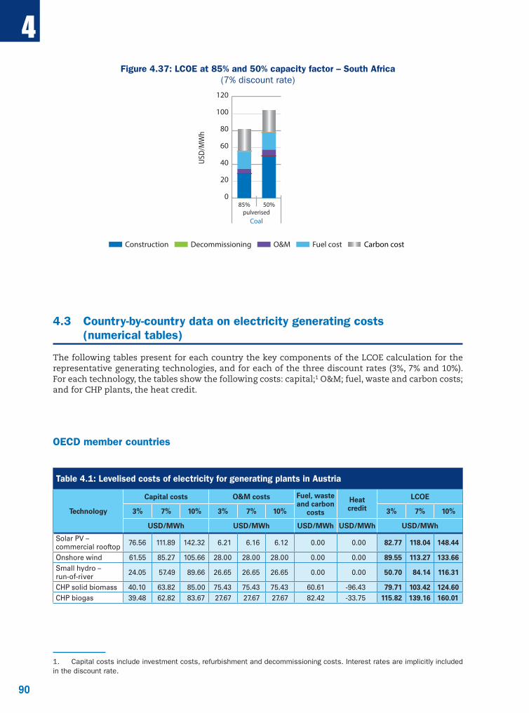
90

4

90

Figure 4.37: LCOE at 85% and 50% capacity factor – South Africa (7% discount rate)

USD

/MW

hpulverised

Coal

DecommissioningConstruction Carbon costO&M Fuel cost

0

20

40

60

80

100

120

50%85%

4.3 Country-by-country data on electricity generating costs (numerical tables)

The following tables present for each country the key components of the LCOE calculation for the representative generating technologies, and for each of the three discount rates (3%, 7% and 10%). For each technology, the tables show the following costs: capital;1 O&M; fuel, waste and carbon costs; and for CHP plants, the heat credit.

OECD member countries

Table 4.1: Levelised costs of electricity for generating plants in Austria

Technology

Capital costs O&M costs Fuel, waste and carbon

costs

Heat credit

LCOE

3% 7% 10% 3% 7% 10% 3% 7% 10%

USD/MWh USD/MWh USD/MWh USD/MWh USD/MWh

Solar PV – commercial rooftop 76.56 111.89 142.32 6.21 6.16 6.12 0.00 0.00 82.77 118.04 148.44

Onshore wind 61.55 85.27 105.66 28.00 28.00 28.00 0.00 0.00 89.55 113.27 133.66Small hydro – run-of-river 24.05 57.49 89.66 26.65 26.65 26.65 0.00 0.00 50.70 84.14 116.31

CHP solid biomass 40.10 63.82 85.00 75.43 75.43 75.43 60.61 -96.43 79.71 103.42 124.60CHP biogas 39.48 62.82 83.67 27.67 27.67 27.67 82.42 -33.75 115.82 139.16 160.01

1. Capital costs include investment costs, refurbishment and decommissioning costs. Interest rates are implicitly included in the discount rate.

91

4

91

Table 4.2: Levelised costs of electricity for generating plants in Belgium

Technology

Capital costs O&M costs Fuel, waste and carbon

costs

Heat credit

LCOE

3% 7% 10% 3% 7% 10% 3% 7% 10%

USD/MWh USD/MWh USD/MWh USD/MWh USD/MWh

CCGT 9.86 13.94 17.52 3.97 3.97 3.97 84.70 0.00 98.54 102.61 106.19OCGT 8.74 12.35 15.52 3.97 3.97 3.97 114.92 0.00 127.63 131.24 134.41Coal – ultra-supercritical 15.29 26.63 37.30 8.00 8.00 8.00 48.72 0.00 72.00 83.35 94.02

Nuclear – gen III projects 27.44 60.17 92.81 13.55 13.55 13.55 10.46 0.00 51.45 84.17 116.81

Solar PV – residential rooftop 167.62 233.98 289.98 22.00 21.87 21.78 0.00 0.00 189.62 255.85 311.77

Solar PV – commercial rooftop 120.29 167.91 208.11 22.00 21.87 21.78 0.00 0.00 142.29 189.78 229.89

Onshore wind 71.22 98.66 122.25 26.67 26.67 26.67 0.00 0.00 97.89 125.33 148.92Offshore wind 99.24 137.48 170.35 53.33 53.33 53.33 0.00 0.00 152.57 190.81 223.68

Table 4.3: Levelised costs of electricity for generating plants in Denmark

Technology

Capital costs O&M costs Fuel, waste and carbon

costs

Heat credit

LCOE

3% 7% 10% 3% 7% 10% 3% 7% 10%

USD/MWh USD/MWh USD/MWh USD/MWh USD/MWh

Solar PV – residential rooftop 109.35 177.19 235.65 2.23 2.21 2.19 0.00 0.00 111.58 179.39 237.84

Solar PV – commercial rooftop 86.40 140.00 186.20 1.76 1.74 1.72 0.00 0.00 88.16 141.74 187.92

Solar PV – large, ground-mounted 76.48 123.93 164.82 1.56 1.54 1.53 0.00 0.00 78.04 125.47 166.35

Onshore wind 40.04 56.56 71.10 14.26 14.26 14.26 0.00 0.00 54.30 70.82 85.36Offshore wind 70.80 108.62 143.11 27.23 27.23 27.23 0.00 0.00 98.02 135.85 170.33CHP medium – wood chips 78.73 133.11 185.57 15.93 15.93 15.93 119.55 -85.19 129.01 183.40 235.86

CHP medium – straw 88.83 141.96 192.88 23.38 23.38 23.38 103.46 -79.66 136.01 189.14 240.06

CHP medium – natural gas 13.75 20.68 26.85 4.63 4.63 4.63 110.00 -33.69 94.69 101.63 107.79

CHP large – wood pellets 31.59 58.76 84.93 21.79 21.79 21.79 119.54 -33.06 139.87 167.04 193.20

CHP large – coal 31.59 58.76 84.93 21.79 21.79 21.79 58.18 -33.06 78.51 105.68 131.84CHP large – natural gas 15.85 23.85 30.95 12.75 12.75 12.75 83.02 -18.40 93.22 101.21 108.32

Table 4.4: Levelised costs of electricity for generating plants in Finland

Technology

Capital costs O&M costs Fuel, waste and carbon

costs

Heat credit

LCOE

3% 7% 10% 3% 7% 10% 3% 7% 10%

USD/MWh USD/MWh USD/MWh USD/MWh USD/MWh

Nuclear – ALWR 26.01 57.90 89.41 14.59 14.59 14.59 5.09 0.00 46.13 77.64 109.10

92

4

92

Table 4.5: Levelised costs of electricity for generating plants in France

Technology

Capital costs O&M costs Fuel, waste and carbon

costs

Heat credit

LCOE

3% 7% 10% 3% 7% 10% 3% 7% 10%

USD/MWh USD/MWh USD/MWh USD/MWh USD/MWh

CCGT 7.03 11.41 15.43 6.25 6.25 6.25 79.55 0.00 92.83 97.21 101.23Nuclear – ALWR 27.31 59.98 92.54 13.33 13.33 13.33 9.33 0.00 49.98 82.64 115.21Solar PV – residential rooftop 172.93 252.74 321.47 40.96 40.59 40.35 0.00 0.00 213.89 293.32 361.82

Solar PV – commercial rooftop 92.48 135.16 171.92 40.96 40.59 40.35 0.00 0.00 133.44 175.75 212.27

Solar PV – large, ground-mounted 66.40 97.04 123.43 37.81 37.46 37.25 0.00 0.00 104.21 134.50 160.68

Onshore wind 46.74 69.14 88.49 22.15 22.15 22.15 0.00 0.00 68.90 91.29 110.64Offshore wind 92.97 142.79 188.18 39.95 39.95 39.95 0.00 0.00 132.92 182.75 228.14Note: Nuclear costs are estimates for a series of plants commissioned at the 2030 horizon. Solar PV – residential rooftop costs include additional costs specific to roof-integrated solar-systems.

Table 4.6: Levelised costs of electricity for generating plants in Germany

Technology

Capital costs O&M costs Fuel, waste and carbon

costs

Heat credit

LCOE

3% 7% 10% 3% 7% 10% 3% 7% 10%

USD/MWh USD/MWh USD/MWh USD/MWh USD/MWh

CCGT 6.88 10.95 14.59 7.71 7.71 7.71 83.90 0.00 98.49 102.56 106.20OCGT 4.37 6.57 8.53 4.39 4.39 4.39 126.15 0.00 134.91 137.11 139.07Coal – hard coal 9.51 18.03 25.97 9.14 9.14 9.14 48.36 0.00 67.01 75.53 83.47Coal – lignite 11.89 22.54 32.46 11.07 11.07 11.07 43.08 0.00 66.04 76.69 86.61Solar PV – residential rooftop 128.10 190.01 242.81 33.46 33.21 33.06 0.00 0.00 161.56 223.23 275.87

Solar PV – commercial rooftop 92.47 137.16 175.27 24.15 23.98 23.86 0.00 0.00 116.62 161.13 199.13

Solar PV – large, ground-mounted 72.96 108.23 138.30 19.06 18.92 18.83 0.00 0.00 92.02 127.14 157.13

Onshore wind 42.49 58.86 72.93 34.67 34.67 34.67 0.00 0.00 77.15 93.53 107.60Offshore wind 96.97 134.34 166.46 49.33 49.33 49.33 0.00 0.00 146.31 183.68 215.80Small hydro – run-of-river 77.68 171.98 265.42 41.10 41.10 41.10 0.00 0.00 118.78 213.08 306.51

Large hydro – run-of-river 47.69 105.76 163.41 17.40 17.40 17.40 0.00 0.00 65.08 123.16 180.80

CHP engine – biogas (digester) 35.27 50.28 62.77 32.93 32.93 32.93 0.00 -43.20 25.00 40.01 52.50

CHP engine – biogas 51.63 80.41 103.38 59.74 59.74 59.74 0.00 -51.75 59.62 88.40 111.37CHP engine – mine gas 22.06 31.75 39.75 28.55 28.55 28.55 0.00 -46.20 4.40 14.09 22.10

CHP steam turbine – solid biomass 81.35 114.93 144.48 41.11 41.11 41.11 106.88 -150.75 78.59 112.16 141.72

CHP geothermal 186.64 290.14 392.66 77.58 77.58 77.58 0.00 -31.36 232.86 336.35 438.88

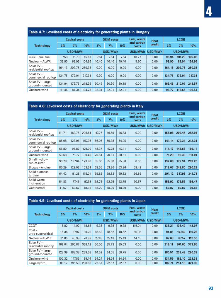
93

4

93

Table 4.7: Levelised costs of electricity for generating plants in Hungary

Technology

Capital costs O&M costs Fuel, waste and carbon

costs

Heat credit

LCOE

3% 7% 10% 3% 7% 10% 3% 7% 10%

USD/MWh USD/MWh USD/MWh USD/MWh USD/MWh

CCGT (dual fuel) 7.53 11.79 15.67 7.64 7.64 7.64 81.77 0.00 96.94 101.20 105.08Nuclear – ALWR 33.90 69.95 104.95 10.40 10.40 10.40 9.60 0.00 53.90 89.94 124.95Solar PV – residential rooftop 164.13 209.78 250.35 0.00 0.00 0.00 0.00 0.00 164.13 209.78 250.35

Solar PV – commercial rooftop 134.76 179.04 217.31 0.00 0.00 0.00 0.00 0.00 134.76 179.04 217.31

Solar PV – large, ground-mounted 134.94 179.76 218.39 30.49 30.30 30.18 0.00 0.00 165.43 210.07 248.57

Onshore wind 61.46 84.34 104.23 32.31 32.31 32.31 0.00 0.00 93.77 116.65 136.54

Table 4.8: Levelised costs of electricity for generating plants in Italy

Technology

Capital costs O&M costs Fuel, waste and carbon

costs

Heat credit

LCOE

3% 7% 10% 3% 7% 10% 3% 7% 10%

USD/MWh USD/MWh USD/MWh USD/MWh USD/MWh

Solar PV – residential rooftop 111.71 162.75 206.61 47.27 46.69 46.33 0.00 0.00 158.98 209.45 252.94

Solar PV – commercial rooftop 85.08 123.96 157.36 56.06 55.38 54.95 0.00 0.00 141.14 179.34 212.31

Solar PV – large, ground-mounted 65.80 95.87 121.70 48.37 47.78 47.41 0.00 0.00 114.17 143.65 169.11

Onshore wind 50.68 71.77 90.40 20.61 20.61 20.61 0.00 0.00 71.29 92.38 111.01Small hydro – run-of-river 96.78 137.64 173.90 35.30 35.30 35.30 0.00 0.00 132.08 172.94 209.20

Biogas – engine 86.29 122.02 153.51 63.36 63.36 63.36 63.42 0.00 213.07 248.80 280.29Solid biomass – turbine 64.42 91.28 115.01 69.82 69.82 69.82 156.89 0.00 291.12 317.98 341.71

Solid waste incineration 54.83 77.46 97.38 192.75 192.75 192.75 -90.67 0.00 156.92 179.55 199.47

Geothermal 41.67 62.67 81.35 18.20 18.20 18.20 0.00 0.00 59.87 80.87 99.55

Table 4.9: Levelised costs of electricity for generating plants in Japan

Technology

Capital costs O&M costs Fuel, waste and carbon

costs

Heat credit

LCOE

3% 7% 10% 3% 7% 10% 3% 7% 10%

USD/MWh USD/MWh USD/MWh USD/MWh USD/MWh

CCGT 8.82 14.02 18.68 9.38 9.38 9.38 115.01 0.00 133.21 138.42 143.07Coal – ultra-supercritical 15.36 27.97 39.79 18.52 18.52 18.52 60.93 0.00 94.81 107.42 119.25

Nuclear – ALWR 21.05 45.99 70.92 27.43 27.43 27.43 14.15 0.00 62.63 87.57 112.50Solar PV – residential rooftop 182.04 265.87 338.12 36.06 35.73 35.53 0.00 0.00 218.11 301.60 373.65

Solar PV – large, ground-mounted 128.99 188.38 239.58 51.52 51.05 50.75 0.00 0.00 180.51 239.43 290.33

Onshore wind 100.32 147.86 189.14 34.24 34.24 34.24 0.00 0.00 134.56 182.10 223.38Large hydro 80.17 191.59 298.82 22.57 22.57 22.57 0.00 0.00 102.74 214.16 321.39

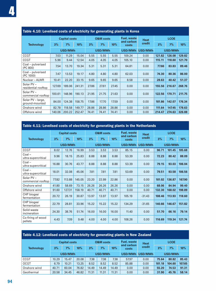
94

4

94

Table 4.10: Levelised costs of electricity for generating plants in Korea

Technology

Capital costs O&M costs Fuel, waste and carbon

costs

Heat credit

LCOE

3% 7% 10% 3% 7% 10% 3% 7% 10%

USD/MWh USD/MWh USD/MWh USD/MWh USD/MWh

CCGT 7.03 11.29 15.04 5.55 5.55 5.55 109.24 0.00 121.82 126.08 129.82CCGT 5.96 9.44 12.54 4.05 4.05 4.05 105.10 0.00 115.11 118.60 121.70Coal – pulverised (PC 800) 7.54 13.70 19.34 5.31 5.31 5.31 64.81 0.00 77.66 83.83 89.46

Coal – pulverised (PC 1000) 7.47 13.53 19.17 4.80 4.80 4.80 62.03 0.00 74.30 80.36 86.00

Nuclear – ALWR 10.41 22.20 33.15 9.65 9.65 9.65 8.58 0.00 28.63 40.42 51.37Solar PV – residential rooftop 127.69 189.06 241.31 27.86 27.61 27.45 0.00 0.00 155.56 216.67 268.76

Solar PV – commercial rooftop 100.61 148.96 190.13 21.95 21.75 21.63 0.00 0.00 122.56 170.71 211.75

Solar PV – large, ground-mounted 84.00 124.38 158.75 17.86 17.70 17.59 0.00 0.00 101.86 142.07 176.34

Onshore wind 82.78 118.58 149.77 28.86 28.86 28.86 0.00 0.00 111.64 147.45 178.63Offshore wind 140.06 200.22 252.47 74.41 74.41 74.41 0.00 0.00 214.47 274.63 326.88

Table 4.11: Levelised costs of electricity for generating plants in the Netherlands

Technology

Capital costs O&M costs Fuel, waste and carbon

costs

Heat credit

LCOE

3% 7% 10% 3% 7% 10% 3% 7% 10%

USD/MWh USD/MWh USD/MWh USD/MWh USD/MWh

CCGT 8.02 12.76 16.99 3.53 3.53 3.53 85.15 0.00 96.71 101.45 105.68Coal – ultra-supercritical 9.96 18.15 25.83 8.88 8.88 8.88 53.39 0.00 72.23 80.42 88.09

Coal – ultra-supercritical 16.88 30.76 43.77 8.88 8.88 8.88 53.39 0.00 79.15 93.03 106.04

Coal – ultra-supercritical 18.01 32.08 45.06 7.81 7.81 7.81 53.69 0.00 79.51 93.58 106.56

Solar PV – commercial rooftop 77.82 113.88 145.05 23.20 22.99 22.86 0.00 0.00 101.02 136.87 167.90

Onshore wind 41.80 58.69 73.15 26.26 26.26 26.26 0.00 0.00 68.06 84.94 99.40Offshore wind 91.60 127.31 158.19 40.71 40.71 40.71 0.00 0.00 132.30 168.02 198.89CHP biogas/fermentation 20.72 26.19 30.87 13.97 13.97 13.97 105.19 -31.43 108.46 113.93 118.60

CHP biogas/fermentation 22.79 28.81 33.96 15.22 15.22 15.22 134.29 -31.65 140.66 146.67 151.82

Solid waste incineration 24.30 38.76 51.74 16.00 16.00 16.00 11.40 0.00 51.70 66.16 79.14

Co-firing of wood pellets 4.43 7.09 9.48 4.00 4.00 4.00 108.26 0.00 116.69 119.34 121.74

Table 4.12: Levelised costs of electricity for generating plants in New Zealand

Technology

Capital costs O&M costs Fuel, waste and carbon

costs

Heat credit

LCOE

3% 7% 10% 3% 7% 10% 3% 7% 10%

USD/MWh USD/MWh USD/MWh USD/MWh USD/MWh

CCGT 10.29 15.47 20.08 7.38 7.38 7.38 57.97 0.00 75.64 80.82 85.43OCGT 6.79 10.21 13.25 8.52 8.52 8.52 85.88 0.00 101.18 104.60 107.65Onshore wind 40.71 60.04 76.82 14.49 14.49 14.49 0.00 0.00 55.20 74.53 91.31Geothermal 20.58 34.45 46.82 11.31 11.31 11.31 0.00 0.00 31.90 45.76 58.14

95

4

95

Table 4.13: Levelised costs of electricity for generating plants in Portugal

Technology

Capital costs O&M costs Fuel, waste and carbon

costs

Heat credit

LCOE

3% 7% 10% 3% 7% 10% 3% 7% 10%

USD/MWh USD/MWh USD/MWh USD/MWh USD/MWh

CCGT 8.51 12.80 16.61 6.24 6.24 6.24 83.90 0.00 98.65 102.93 106.75Coal – pulverised 18.44 30.55 41.94 6.16 6.16 6.16 53.68 0.00 78.28 90.39 101.77Coal – pulverised 22.33 36.99 50.76 14.53 14.53 14.53 48.41 0.00 85.27 99.93 113.71Solar PV – residential rooftop 77.28 112.95 143.67 18.86 18.69 18.58 0.00 0.00 96.14 131.64 162.25

Solar PV – commercial rooftop 55.20 80.68 102.62 18.86 18.69 18.58 0.00 0.00 74.06 99.37 121.20

Solar PV – large, ground-mounted 57.35 83.81 106.61 17.81 17.65 17.55 0.00 0.00 75.16 101.46 124.16

Onshore wind 42.77 63.08 80.70 18.26 18.26 18.26 0.00 0.00 61.03 81.34 98.97Offshore wind 91.39 134.78 172.45 88.36 88.36 88.36 0.00 0.00 179.75 223.14 260.81Large hydro – reservoir 72.89 171.56 267.18 16.65 16.65 16.65 0.00 0.00 89.54 188.22 283.83

Large hydro – pumped storage 56.32 132.57 206.45 12.14 12.14 12.14 0.00 0.00 68.46 144.71 218.59

Table 4.14: Levelised costs of electricity for generating plants in the Slovak Republic

Technology

Capital costs O&M costs Fuel, waste and carbon

costs

Heat credit

LCOE

3% 7% 10% 3% 7% 10% 3% 7% 10%

USD/MWh USD/MWh USD/MWh USD/MWh USD/MWh

Nuclear – LWR 31.30 61.35 93.88 10.17 10.17 10.17 12.43 0.00 53.90 83.95 116.48

Table 4.15: Levelised costs of electricity for generating plants in Spain

Technology

Capital costs O&M costs Fuel, waste and carbon

costs

Heat credit

LCOE

3% 7% 10% 3% 7% 10% 3% 7% 10%

USD/MWh USD/MWh USD/MWh USD/MWh USD/MWh

Solar PV – residential rooftop 64.99 100.43 131.11 35.61 35.59 35.58 0.00 0.00 100.60 136.02 166.70

Solar PV – commercial rooftop 53.61 82.85 108.16 49.35 49.17 49.05 0.00 0.00 102.97 132.01 157.21

Solar PV – large, ground-mounted 41.57 64.35 84.12 45.75 45.57 45.45 0.00 0.00 87.33 109.92 129.57

Solar thermal (CSP) – no storage 175.93 260.88 335.14 87.46 87.46 87.46 0.00 0.00 263.39 348.35 422.60

Onshore wind 53.65 74.32 92.09 27.86 27.86 27.86 0.00 0.00 81.51 102.19 119.96Small hydro – run-of-river 45.66 70.06 92.30 38.40 38.40 38.40 0.00 0.00 84.06 108.46 130.70

Small hydro – reservoir 28.30 42.56 55.25 38.40 38.40 38.40 0.00 0.00 66.70 80.96 93.65

Large hydro – run-of-river 32.79 50.32 66.29 32.40 32.40 32.40 0.00 0.00 65.20 82.72 98.70

Large hydro – reservoir 20.35 30.61 39.73 0.00 0.00 0.00 0.00 0.00 20.35 30.61 39.73

Biomass – turbine 37.25 57.15 75.30 41.22 41.22 41.22 73.41 0.00 151.88 171.78 189.93Biogas – engine 25.78 38.03 48.65 52.13 52.13 52.13 0.00 0.00 77.92 90.16 100.79Biogas – engine 51.98 76.66 98.08 60.52 60.52 60.52 0.00 0.00 112.49 137.17 158.60Solid waste incineration – turbine

104.94 161.00 212.12 124.34 124.34 124.34 0.00 0.00 229.28 285.34 336.46

CHP engine 94.35 144.76 190.72 36.29 36.29 36.29 69.77 -41.17 159.25 209.66 255.62CHP gas turbine 14.29 21.50 27.91 31.40 31.40 31.40 65.69 -82.46 28.92 36.12 42.53

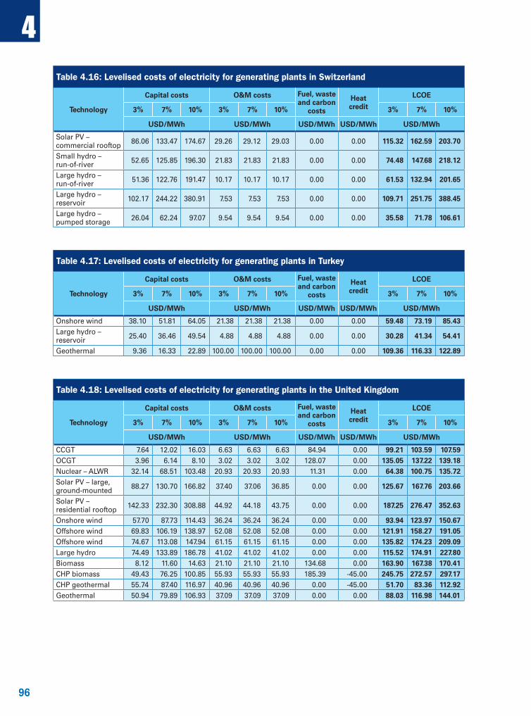
96

4

96

Table 4.16: Levelised costs of electricity for generating plants in Switzerland

Technology

Capital costs O&M costs Fuel, waste and carbon

costs

Heat credit

LCOE

3% 7% 10% 3% 7% 10% 3% 7% 10%

USD/MWh USD/MWh USD/MWh USD/MWh USD/MWh

Solar PV – commercial rooftop 86.06 133.47 174.67 29.26 29.12 29.03 0.00 0.00 115.32 162.59 203.70

Small hydro – run-of-river 52.65 125.85 196.30 21.83 21.83 21.83 0.00 0.00 74.48 147.68 218.12

Large hydro – run-of-river 51.36 122.76 191.47 10.17 10.17 10.17 0.00 0.00 61.53 132.94 201.65

Large hydro – reservoir 102.17 244.22 380.91 7.53 7.53 7.53 0.00 0.00 109.71 251.75 388.45

Large hydro – pumped storage 26.04 62.24 97.07 9.54 9.54 9.54 0.00 0.00 35.58 71.78 106.61

Table 4.17: Levelised costs of electricity for generating plants in Turkey

Technology

Capital costs O&M costs Fuel, waste and carbon

costs

Heat credit

LCOE

3% 7% 10% 3% 7% 10% 3% 7% 10%

USD/MWh USD/MWh USD/MWh USD/MWh USD/MWh

Onshore wind 38.10 51.81 64.05 21.38 21.38 21.38 0.00 0.00 59.48 73.19 85.43Large hydro – reservoir 25.40 36.46 49.54 4.88 4.88 4.88 0.00 0.00 30.28 41.34 54.41

Geothermal 9.36 16.33 22.89 100.00 100.00 100.00 0.00 0.00 109.36 116.33 122.89

Table 4.18: Levelised costs of electricity for generating plants in the United Kingdom

Technology

Capital costs O&M costs Fuel, waste and carbon

costs

Heat credit

LCOE

3% 7% 10% 3% 7% 10% 3% 7% 10%

USD/MWh USD/MWh USD/MWh USD/MWh USD/MWh

CCGT 7.64 12.02 16.03 6.63 6.63 6.63 84.94 0.00 99.21 103.59 107.59OCGT 3.96 6.14 8.10 3.02 3.02 3.02 128.07 0.00 135.05 137.22 139.18Nuclear – ALWR 32.14 68.51 103.48 20.93 20.93 20.93 11.31 0.00 64.38 100.75 135.72Solar PV – large, ground-mounted 88.27 130.70 166.82 37.40 37.06 36.85 0.00 0.00 125.67 167.76 203.66

Solar PV – residential rooftop 142.33 232.30 308.88 44.92 44.18 43.75 0.00 0.00 187.25 276.47 352.63

Onshore wind 57.70 87.73 114.43 36.24 36.24 36.24 0.00 0.00 93.94 123.97 150.67Offshore wind 69.83 106.19 138.97 52.08 52.08 52.08 0.00 0.00 121.91 158.27 191.05Offshore wind 74.67 113.08 147.94 61.15 61.15 61.15 0.00 0.00 135.82 174.23 209.09Large hydro 74.49 133.89 186.78 41.02 41.02 41.02 0.00 0.00 115.52 174.91 227.80Biomass 8.12 11.60 14.63 21.10 21.10 21.10 134.68 0.00 163.90 167.38 170.41CHP biomass 49.43 76.25 100.85 55.93 55.93 55.93 185.39 -45.00 245.75 272.57 297.17CHP geothermal 55.74 87.40 116.97 40.96 40.96 40.96 0.00 -45.00 51.70 83.36 112.92Geothermal 50.94 79.89 106.93 37.09 37.09 37.09 0.00 0.00 88.03 116.98 144.01

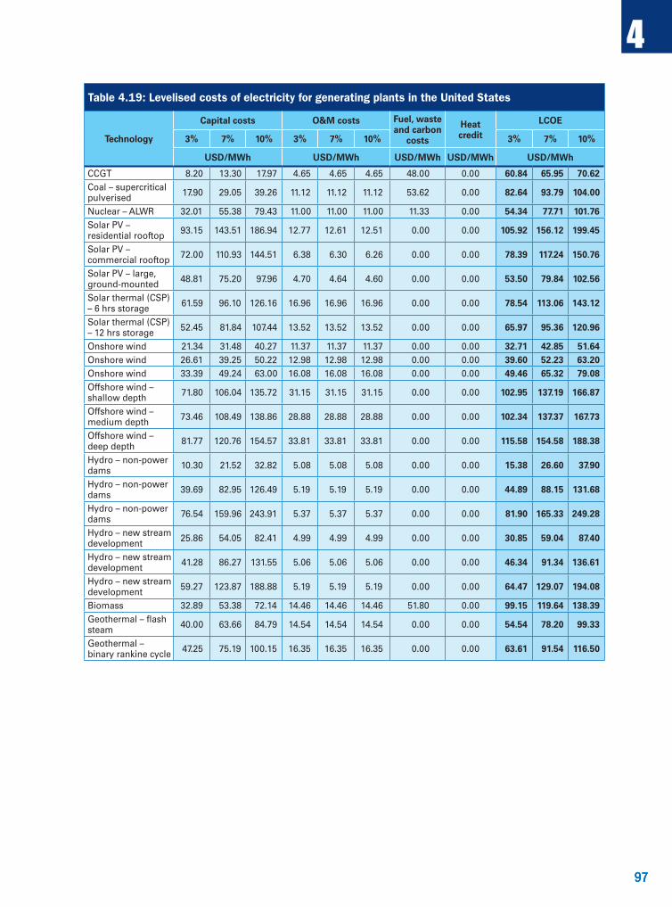
97

4

97

Table 4.19: Levelised costs of electricity for generating plants in the United States

Technology

Capital costs O&M costs Fuel, waste and carbon

costs

Heat credit

LCOE

3% 7% 10% 3% 7% 10% 3% 7% 10%

USD/MWh USD/MWh USD/MWh USD/MWh USD/MWh

CCGT 8.20 13.30 17.97 4.65 4.65 4.65 48.00 0.00 60.84 65.95 70.62Coal – supercritical pulverised 17.90 29.05 39.26 11.12 11.12 11.12 53.62 0.00 82.64 93.79 104.00

Nuclear – ALWR 32.01 55.38 79.43 11.00 11.00 11.00 11.33 0.00 54.34 77.71 101.76Solar PV – residential rooftop 93.15 143.51 186.94 12.77 12.61 12.51 0.00 0.00 105.92 156.12 199.45

Solar PV – commercial rooftop 72.00 110.93 144.51 6.38 6.30 6.26 0.00 0.00 78.39 117.24 150.76

Solar PV – large, ground-mounted 48.81 75.20 97.96 4.70 4.64 4.60 0.00 0.00 53.50 79.84 102.56

Solar thermal (CSP) – 6 hrs storage 61.59 96.10 126.16 16.96 16.96 16.96 0.00 0.00 78.54 113.06 143.12

Solar thermal (CSP) – 12 hrs storage 52.45 81.84 107.44 13.52 13.52 13.52 0.00 0.00 65.97 95.36 120.96

Onshore wind 21.34 31.48 40.27 11.37 11.37 11.37 0.00 0.00 32.71 42.85 51.64Onshore wind 26.61 39.25 50.22 12.98 12.98 12.98 0.00 0.00 39.60 52.23 63.20Onshore wind 33.39 49.24 63.00 16.08 16.08 16.08 0.00 0.00 49.46 65.32 79.08Offshore wind – shallow depth 71.80 106.04 135.72 31.15 31.15 31.15 0.00 0.00 102.95 137.19 166.87

Offshore wind – medium depth 73.46 108.49 138.86 28.88 28.88 28.88 0.00 0.00 102.34 137.37 167.73

Offshore wind – deep depth 81.77 120.76 154.57 33.81 33.81 33.81 0.00 0.00 115.58 154.58 188.38

Hydro – non-power dams 10.30 21.52 32.82 5.08 5.08 5.08 0.00 0.00 15.38 26.60 37.90

Hydro – non-power dams 39.69 82.95 126.49 5.19 5.19 5.19 0.00 0.00 44.89 88.15 131.68

Hydro – non-power dams 76.54 159.96 243.91 5.37 5.37 5.37 0.00 0.00 81.90 165.33 249.28

Hydro – new stream development 25.86 54.05 82.41 4.99 4.99 4.99 0.00 0.00 30.85 59.04 87.40

Hydro – new stream development 41.28 86.27 131.55 5.06 5.06 5.06 0.00 0.00 46.34 91.34 136.61

Hydro – new stream development 59.27 123.87 188.88 5.19 5.19 5.19 0.00 0.00 64.47 129.07 194.08

Biomass 32.89 53.38 72.14 14.46 14.46 14.46 51.80 0.00 99.15 119.64 138.39Geothermal – flash steam 40.00 63.66 84.79 14.54 14.54 14.54 0.00 0.00 54.54 78.20 99.33

Geothermal – binary rankine cycle 47.25 75.19 100.15 16.35 16.35 16.35 0.00 0.00 63.61 91.54 116.50

98

4

98

Non-OECD countries

Table 4.20: Levelised costs of electricity for generating plants in Brazil

Technology

Capital costs O&M costs Fuel, waste and carbon

costs

Heat credit

LCOE

3% 7% 10% 3% 7% 10% 3% 7% 10%

USD/MWh USD/MWh USD/MWh USD/MWh USD/MWh

Large hydro – run-of-river 13.34 26.25 38.21 9.00 9.00 9.00 0.00 0.00 22.34 35.25 47.21

Large hydro – run-of-river 42.71 69.85 94.93 8.89 8.89 8.89 0.00 0.00 51.60 78.74 103.82

Large hydro – run-of-river 10.62 21.53 32.07 9.18 9.18 9.18 0.00 0.00 19.79 30.71 41.24

Large hydro 13.33 26.31 38.41 8.94 8.94 8.94 0.00 0.00 22.28 35.26 47.35

Table 4.21: Levelised costs of electricity for generating plants in China

Technology

Capital costs O&M costs Fuel, waste and carbon

costs

Heat credit

LCOE

3% 7% 10% 3% 7% 10% 3% 7% 10%

USD/MWh USD/MWh USD/MWh USD/MWh USD/MWh

CCGT 4.43 7.06 9.40 3.25 3.25 3.25 82.48 0.00 90.17 92.79 95.13Coal – ultra-supercritical 5.00 9.11 12.96 4.07 4.07 4.07 64.54 0.00 73.61 77.72 81.57

Nuclear – ALWR 14.12 30.96 47.76 7.32 7.32 7.32 9.33 0.00 30.77 47.61 64.40Nuclear – ALWR 9.76 21.39 33.00 6.50 6.50 6.50 9.33 0.00 25.59 37.23 48.83Solar PV – commercial rooftop 42.73 62.44 79.43 16.26 16.26 16.26 0.00 0.00 58.99 78.70 95.69

Solar PV – large, ground-mounted 38.58 56.38 71.72 16.26 16.26 16.26 0.00 0.00 54.84 72.64 87.98

Onshore wind 36.21 50.16 62.15 9.76 9.76 9.76 0.00 0.00 45.96 59.92 71.91Onshore wind 42.24 58.52 72.51 9.76 9.76 9.76 0.00 0.00 52.00 68.28 82.27Large hydro – reservoir 4.78 11.43 17.83 10.57 10.57 10.57 0.00 0.00 15.35 22.00 28.39

Table 4.22: Levelised costs of electricity for generating plants in South Africa

Technology

Capital costs O&M costs Fuel, waste and carbon

costs

Heat credit

LCOE

3% 7% 10% 3% 7% 10% 3% 7% 10%

USD/MWh USD/MWh USD/MWh USD/MWh USD/MWh

Coal – pulverised 12.45 29.21 46.93 5.41 5.41 5.41 47.45 0.00 65.31 82.07 99.79Solar thermal (CSP) – molten salt storage

86.21 139.03 190.03 53.06 53.06 53.06 0.00 0.00 139.27 192.08 243.09

Onshore wind 63.38 88.07 109.32 13.86 13.86 13.86 0.00 0.00 77.24 101.93 123.19

99

5

99

Chapter

History of Projected Costs of Generating Electricity, 1981-2015

5.1 Introduction

The series of Projected Costs of Generating Electricity reports has been produced jointly by the International Energy Agency (IEA) and the Nuclear Energy Agency (NEA) of the OECD every five to ten years since 1981 to evaluate the levelised cost of electricity generation for a variety of technologies and fuel sources. The reports use input data provided by participating countries in the form of a questionnaire response. The levelised cost methodology applied is agreed upon by nationally appointed experts from participating countries and contains many basic default assumptions reflective of the current situation in electricity generation technologies and markets.

Presented below is a review of this series of reports, with particular emphasis on the evolution of the levelised cost methodology and key trends present in each report. This is meant to provide insight for the historical development of the current electricity generating costs (EGC) model and levelised cost methodology. Final levelised costs for mainstream technologies for each edition of the report are presented in comparison with the updated results presented in this edition for a better understanding of historic trends in projected costs across several decades of analysis.

It should be emphasised that the numbers provided should be treated in the broader context of the overall development of electricity generation costs rather than country- or technology-specific trends. Several caveats should be noted when considering these values. First, because of changes in relative exchange rates, simply adjusting final levelised costs reported in US dollars (USD) from each edition for inflation fails to account for historical developments in currency markets and relative purchasing powers. Ideally, one could present the results of two methods for inflation adjustment: i)  where the levelised cost is reported in historical US dollars, then converting this to current US dollars, and ii) where the levelised cost is reported in historical national currency units (NCUs) and adjusted to current NCUs, then converted to current US dollars on the basis of present-day exchange rates.

Second, changes in methodology make it difficult, if not impossible, to make cross-report comparisons. As the average lifetime and lifetime capacity factor assumptions increase, the cost of the plant is distributed over a longer operating period and thus the cost per MWh decreases. However, changes to the levelised cost formula, such as incorporation of carbon prices, increase the cost of fossil fuels relative to nuclear power. Third, each edition assumes a plant that is state-of-the-art technology at the time of the report. Over the course of the Projected Costs series, the progress of technological development implies that the plants being considered in the 1981 edition may be extremely different from those being considered in the 2015 edition. It is thus difficult to make cross-report comparisons.

100

5

100

5.2 Previous editions

Projected Costs of Generating Electricity, 1st Edition, 1981

The first report of Projected Costs, published in 1981 by the NEA (i.e. without IEA participation), established the reference framework and methodology for calculation of levelised costs. Particular emphasis was paid to including all direct costs incurred in association with nuclear power. The report made use of a 5% discount rate and currency values in a common European currency unit (ECU). This first report received participation from 12 countries and compared two energy sources: nuclear and coal. It concluded that nuclear energy was cheaper than coal-generated electricity in all cases except subsections of the United States where coal was found to be particularly cheap.

Projected Costs of Generating Electricity, 2nd Edition, 1984

The sequel to the original report was published by the NEA three years later. The updated version included data from 17 participating countries on nuclear and coal plants. In this second edition, the reference monetary unit was shifted to the US dollar, and it remains today. Moreover, the 10% discount rate was added for a comparison against the default 5% assumption. Like the original, the 1984 edition found that nuclear energy was substantially cheaper than coal for all countries aside from parts of the United States, where coal prices gave coal power a slim advantage. The advantage of nuclear also diminished for the 10% discount rate.

The primary distinction between this edition and the first one was the shift in reference currency unit as well as the decrease in projected coal prices in most parts of the world. Given the relative appreciation of the US dollar, however, these two effects almost cancelled each other. The economic lifetime was 25 years and the reference lifetime capacity factor was 72%.

Projected Costs of Generating Electricity, 3rd Edition, 1989

The 1989 edition was for the first time jointly produced by the International Energy Agency (IEA) and the NEA and featured data from a total of 18 participating countries, focusing on nuclear and coal technologies. However, analysis of alternative technologies, including renewables, was included in an appendix for reference. As these technologies came into wider use, they featured increasingly prominently in Projected Costs reports. Again, a 30-year lifetime and 72% lifetime capacity factor was assumed. This edition further addressed differences in taxation, subsidy, and externality programmes that could influence generation costs, the cost of decommissioning, and an alternative method of addressing uncertainty based on probability theory.

The third edition concluded that while nuclear energy maintained a significant cost advantage over coal, a projected decrease in future coal prices could lead to coal-powered electricity gaining a narrow advantage for some countries. Natural gas-fired steam plants were considered uncompetitive aside from isolated instances in which projected low gas prices favoured combined-cycle gas turbines (CCGTs).

Projected Costs of Generating Electricity, 4th Edition, 1992

This edition included participation from 22 countries, of which 6 were non-OECD countries. The report was the first to include natural gas-fired plants as well as some renewables in its main analysis. It made use of a default assumption of 30-year operating lifetime and 75% lifetime capacity factor for baseload plants. The report found that there was no clear winner among nuclear, natural gas and coal technologies in all countries because of decreased projected fossil fuel prices, projecting coal-fired power as a serious future baseload contender for the first time. It further concluded that variable renewable technologies were uneconomic except in remote locations and/or especially good conditions.

101

5

101

This update recognised the influence that environmental considerations could have on future generation cost reports. It remarked on these trends as well as on the liberalisation of the energy markets, the status of commitments by OECD member countries to greenhouse gas reductions and new emission control technologies.

Projected Costs of Generating Electricity, 5th Edition, 1998

Given the decreasing popularity of oil in power generation, the fifth edition of the report eliminated this technology from its consideration. The update included in its main analysis the baseload technologies of coal, natural gas and nuclear, with a qualitative discussion of hydropower, biomass and wind. This report featured 14 OECD participating countries and data from 5 non-OECD countries. It concluded that despite increasing competitiveness from natural gas-fired plants, there remained no clear winner among the three prevailing baseload technologies in the most general case, and that renewable energy technologies remained generally uncompetitive compared to coal, natural gas and nuclear plants. Annexes included discussions of environmental protection costs, the influences of market liberalisation and the value of energy diversity and security.

Projected Costs of Generating Electricity, 6th Edition, 2005

The sixth edition analysed submissions from 18 member countries and 3 non-member countries. The methodology extended the default lifetime capacity factor to 85% for coal, natural gas and nuclear plants while maintaining the assumption of a 40-year operating lifetime for coal and nuclear plants, considering the new higher capacity factor as more representative of the average lifetime value for baseload plants. The report found that no single technology was preferred for all instances.

However, increased liberalisation of energy markets was noted to contribute to uncertainty, thus favouring less capital-intensive and more flexible technology options. This edition was the first to include, by request from participating countries, a quantitative analysis of hydropower. It also briefly analysed costs associated with distributed generation, waste incineration and landfill gas, biomass, geothermal and oil plants. It discussed the increasingly important question of incorporating risk in cost estimates. A methodology for analysing the costs of combined heat and power (CHP) plants was outlined. While the annex explored a more detailed method for allocating costs of electricity and heat generation, the model computed the value of total discounted heat generation by using nationally provided figures for the heat value, then subtracting this “heat credit” from the total generating cost.

Projected Costs of Generating Electricity, 7th Edition, 2010

The most recent edition notably included a carbon price of USD 30/tonne of CO2 to reflect policy objectives of reducing greenhouse gas emissions. At the time of the report, only the European Union had implemented a carbon pricing system; however, similar schemes continued to be debated extensively in other countries. Further, even if the price was not explicitly levied on fossil fuel plants, the carbon price included in the model reflected growing pressure to reduce emissions and the effect that possible taxes could have on the current generation choices.

The seventh edition further distinguished onshore wind as a potentially competitive electricity generation source, in part because of strong support from governments seeking to promote renewable energy technologies. In general, the report found that the variability and unpredictability of many renewable technologies, stemming from their relative immaturity, put them at a relative disadvantage compared to more established and stable sources. The report concluded that there is no one technology with a clear advantage on the global or even regional level.

Qualitative discussion, but no quantitative analysis, was given to system integration of non-dispatchable technologies, the current cost of capital and various taxation schemes, the cost of carbon capture and sequestration and the behaviour of energy markets. Uncertainties were noted in future fuel and CO2 prices, financing and overnight cost, decommissioning and waste management costs, and the stability of future electricity prices.

102

5

102

5.3 Country-by-country tables and figures on electricity generating costs for mainstream technologies

As noted previously, given the changes in assumptions and methodology over the several editions of the Projected Costs reports, it is nearly meaningless to compare changes in levelised costs calculated throughout the series. As assumptions, such as average capacity factor and lifetime, have changed, the average cost per unit of generation changed accordingly. Further, updates in technology prevent adequate comparisons between “state-of-the-art” technologies in the 1980s to those that are expected to go on line in 2020.

Most importantly, while it is possible to adjust for inflation the USD/MWh data from each report to 2013 USD/MWh, this does not accurately reflect exchange rates between national currency units and US dollars nor unequal impacts of inflation in each respective country. A truly meaningful analysis of historical trends must not only use a common set of assumptions and methodology throughout, but also consider inflation and allocation of costs between national and imported goods and services for each country.

For reference, costs by country were adjusted for inflation to 2013 USD/MWh and compiled below. Owing to lack of the original responses to country questionnaires, final values from each edition were reported in historical USD/MWh and converted to 2013 USD/MWh using OECD’s published statistics for producer prices, instead of adjusting the historical national currency unit (NCU) to present-day rates and converting to US dollars at current exchange rates. Where multiple values were reported for a country in a single report, the mean is presented. A report of “NA” denotes that the country did not submit a relevant questionnaire for the year being considered.

Regarding natural gas-fired CCGTs, there is no significant difference between the estimates using a 5% discount rate and using a 10% discount between the 1992 and the 2015 editions. There have always been two different groups of countries, e.g. in the 2015 edition: i) Europe and the United States (although with the parallel movement in CCGT estimates in the earlier editions for Canada and the United States, the United States would be better classified as “North America”) and ii) North-East Asia (with Japan estimating CCGT costs from USD 136 to USD 143/MWh as a function of the discount rate, and Korea estimating average CCGT costs from USD 120 to USD 126/MWh); estimated costs for China are between USD 91 and 95/MWh, similar to those in Europe. In this edition, these two different groups of countries split into three different groups: i) the United States with cost estimates between USD 63 and USD 71/MWh; ii) Europe and China with cost estimates between USD 91 and USD 100/MWh, and iii) North-East Asia, with Japan at cost estimates nearly double those in the United States.

Variation in the estimates of coal-fired steam electricity cost does not seem to depend on the discount rate. Since 2005, the cost estimate for coal converged to between USD 71 and USD 101/MWh for a 5% discount rate and between USD 82 and USD 119/MWh for a 10% discount rate. The most noticeable change was in China’s cost estimate to below USD 40/MWh in 2010 to above USD 80/MWh in 2015.

Finally, as one can tell from the tables and figures, the longest running series are for nuclear power and coal at a 5% discount rate from 1981 to 2010. Comparing these with the 2015 values, these costs converge between USD 65/MWh to USD 81/MWh in North America and Europe. On the other hand, the cost estimate for nuclear power at a 5% discount rate is around USD 35/MWh in Korea and China, i.e. half what it is in Europe and the United States. At a 10% discount rate, the cost estimates for nuclear power have been more dispersed over the various editions of the report with one range now between USD 102/MWh in the United States and USD 136/MWh in the United Kingdom, and another range between USD 51/MWh in Korea and USD 57/MWh in China (Figure 5.3b). Again, these are half as much as in Europe and the United States.1

1. These dramatic differences between Northeast Asia and Europe/United States are likely due to: i) lower labour costs, and ii) scale and series economies in construction in China and Korea, the latter of which is supplying many of the larger components to plants being built in the United States.

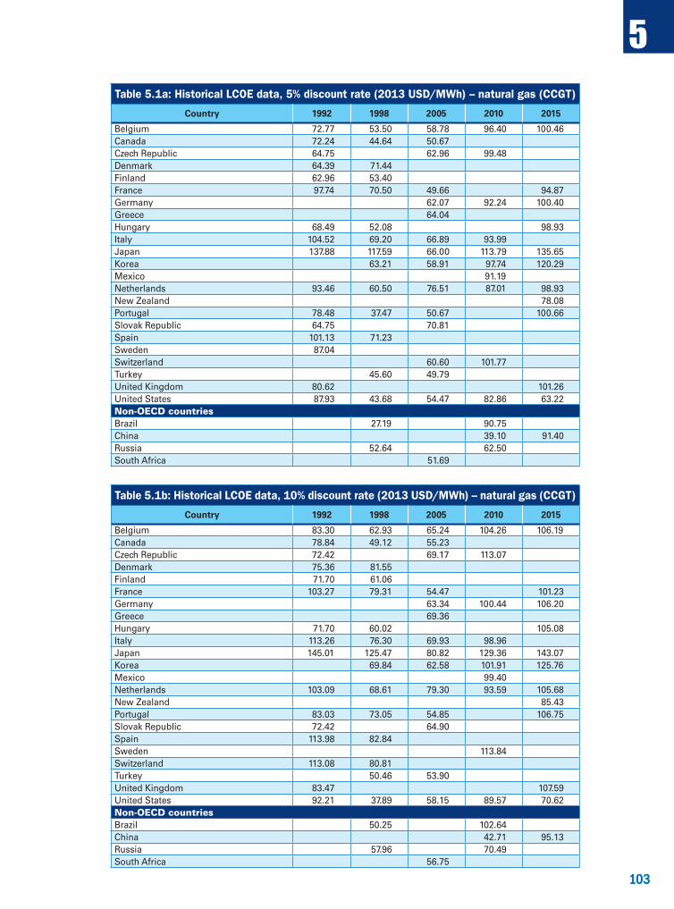
103

5

103

Table 5.1a: Historical LCOE data, 5% discount rate (2013 USD/MWh) – natural gas (CCGT)

Country 1992 1998 2005 2010 2015

Belgium 72.77 53.50 58.78 96.40 100.46Canada 72.24 44.64 50.67Czech Republic 64.75 62.96 99.48Denmark 64.39 71.44Finland 62.96 53.40France 97.74 70.50 49.66 94.87Germany 62.07 92.24 100.40Greece 64.04Hungary 68.49 52.08 98.93Italy 104.52 69.20 66.89 93.99Japan 137.88 117.59 66.00 113.79 135.65Korea 63.21 58.91 97.74 120.29Mexico 91.19Netherlands 93.46 60.50 76.51 87.01 98.93New Zealand 78.08Portugal 78.48 37.47 50.67 100.66Slovak Republic 64.75 70.81Spain 101.13 71.23Sweden 87.04Switzerland 60.60 101.77Turkey 45.60 49.79United Kingdom 80.62 101.26United States 87.93 43.68 54.47 82.86 63.22Non-OECD countriesBrazil 27.19 90.75China 39.10 91.40Russia 52.64 62.50 South Africa 51.69

Table 5.1b: Historical LCOE data, 10% discount rate (2013 USD/MWh) – natural gas (CCGT)

Country 1992 1998 2005 2010 2015

Belgium 83.30 62.93 65.24 104.26 106.19Canada 78.84 49.12 55.23 Czech Republic 72.42 69.17 113.07 Denmark 75.36 81.55 Finland 71.70 61.06 France 103.27 79.31 54.47 101.23Germany 63.34 100.44 106.20Greece 69.36 Hungary 71.70 60.02 105.08Italy 113.26 76.30 69.93 98.96 Japan 145.01 125.47 80.82 129.36 143.07Korea 69.84 62.58 101.91 125.76Mexico 99.40 Netherlands 103.09 68.61 79.30 93.59 105.68New Zealand 85.43Portugal 83.03 73.05 54.85 106.75Slovak Republic 72.42 64.90 Spain 113.98 82.84 Sweden 113.84Switzerland 113.08 80.81Turkey 50.46 53.90 United Kingdom 83.47 107.59United States 92.21 37.89 58.15 89.57 70.62Non-OECD countriesBrazil 50.25 102.64 China 42.71 95.13Russia 57.96 70.49 South Africa 56.75

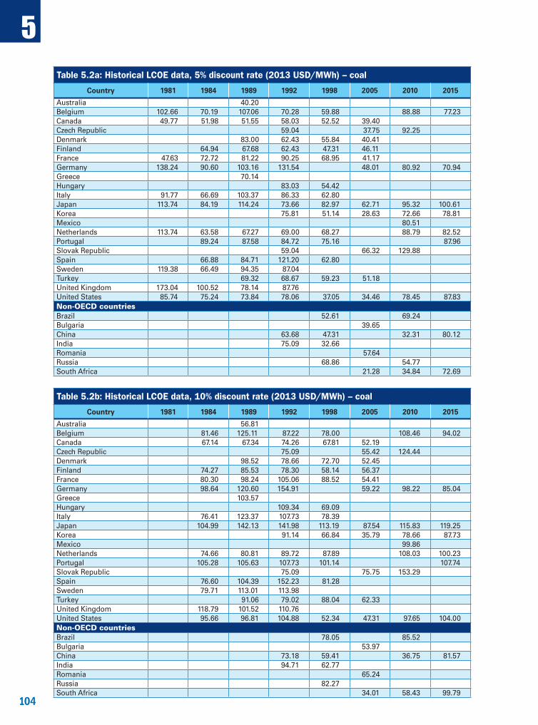
104

5

104

Table 5.2a: Historical LCOE data, 5% discount rate (2013 USD/MWh) – coal

Country 1981 1984 1989 1992 1998 2005 2010 2015

Australia 40.20 Belgium 102.66 70.19 107.06 70.28 59.88 88.88 77.23Canada 49.77 51.98 51.55 58.03 52.52 39.40 Czech Republic 59.04 37.75 92.25 Denmark 83.00 62.43 55.84 40.41 Finland 64.94 67.68 62.43 47.31 46.11 France 47.63 72.72 81.22 90.25 68.95 41.17 Germany 138.24 90.60 103.16 131.54 48.01 80.92 70.94Greece 70.14 Hungary 83.03 54.42 Italy 91.77 66.69 103.37 86.33 62.80 Japan 113.74 84.19 114.24 73.66 82.97 62.71 95.32 100.61Korea 75.81 51.14 28.63 72.66 78.81Mexico 80.51 Netherlands 113.74 63.58 67.27 69.00 68.27 88.79 82.52Portugal 89.24 87.58 84.72 75.16 87.96Slovak Republic 59.04 66.32 129.88 Spain 66.88 84.71 121.20 62.80 Sweden 119.38 66.49 94.35 87.04 Turkey 69.32 68.67 59.23 51.18 United Kingdom 173.04 100.52 78.14 87.76 United States 85.74 75.24 73.84 78.06 37.05 34.46 78.45 87.83Non-OECD countriesBrazil 52.61 69.24 Bulgaria 39.65 China 63.68 47.31 32.31 80.12India 75.09 32.66 Romania 57.64 Russia 68.86 54.77 South Africa 21.28 34.84 72.69

Table 5.2b: Historical LCOE data, 10% discount rate (2013 USD/MWh) – coal

Country 1981 1984 1989 1992 1998 2005 2010 2015

Australia 56.81 Belgium 81.46 125.11 87.22 78.00 108.46 94.02Canada 67.14 67.34 74.26 67.81 52.19 Czech Republic 75.09 55.42 124.44 Denmark 98.52 78.66 72.70 52.45 Finland 74.27 85.53 78.30 58.14 56.37 France 80.30 98.24 105.06 88.52 54.41 Germany 98.64 120.60 154.91 59.22 98.22 85.04Greece 103.57 Hungary 109.34 69.09 Italy 76.41 123.37 107.73 78.39 Japan 104.99 142.13 141.98 113.19 87.54 115.83 119.25Korea 91.14 66.84 35.79 78.66 87.73Mexico 99.86 Netherlands 74.66 80.81 89.72 87.89 108.03 100.23Portugal 105.28 105.63 107.73 101.14 107.74Slovak Republic 75.09 75.75 153.29 Spain 76.60 104.39 152.23 81.28 Sweden 79.71 113.01 113.98 Turkey 91.06 79.02 88.04 62.33 United Kingdom 118.79 101.52 110.76 United States 95.66 96.81 104.88 52.34 47.31 97.65 104.00Non-OECD countriesBrazil 78.05 85.52 Bulgaria 53.97 China 73.18 59.41 36.75 81.57India 94.71 62.77 Romania 65.24 Russia 82.27 South Africa 34.01 58.43 99.79

105

5

105

Table 5.3a: Historical LCOE data, 5% discount rate (2013 USD/MWh) – nuclear

Country 1981 1984 1989 1992 1998 2005 2010 2015

Belgium 73.69 43.36 59.68 64.03 66.08 66.13Canada 49.19 55.80 49.22 53.15 40.32 32.94 Czech Republic 51.55 29.14 75.48 Finland 48.80 56.40 53.69 55.42 34.96 66.52France 60.66 40.44 56.20 58.50 47.93 32.13 61.06 64.63Germany 84.19 53.21 81.83 94.71 36.23 54.08 Hungary 54.04 88.37 70.08Italy 58.33 48.25 82.86 Japan 75.44 61.44 88.81 95.78 85.41 60.81 53.80 73.80Korea 56.63 45.64 28.00 33.54 34.05Netherlands 88.07 48.41 70.96 79.19 45.35 67.92 Slovak Republic 51.55 39.65 67.74 66.68Spain 87.37 61.01 Switzerland 36.48 73.63 Turkey 66.04 48.79 United Kingdom 120.93 65.42 73.43 89.18 80.88United States 84.77 79.08 79.17 76.40 49.48 38.13 52.74 64.81Non-OECD countriesBrazil 51.97 70.66 China 54.76 41.07 34.68 34.57India 64.39 48.79 Romania 47.34 38.76 Russia 39.96 47.50 South Africa

Table 5.3b: Historical LCOE data, 10% discount rate (2013 USD/MWh) – nuclear

Country 1981 1984 1989 1992 1998 2005 2010 2015

Belgium 60.66 87.99 94.89 118.12 116.81Canada 86.00 75.20 102.83 64.52 47.00 Czech Republic 72.06 40.16 124.52 Finland 74.27 87.37 83.30 83.15 53.46 109.10France 54.44 78.76 80.62 73.07 49.79 99.98 115.21Germany 77.58 119.57 138.05 53.33 89.44 Hungary 54.44 73.74 79.73 74.90 55.58 131.63 124.95Italy 66.69 126.96 Japan 85.94 128.39 133.06 118.29 86.90 82.75 112.50Korea 85.53 71.81 40.60 48.96 51.37Netherlands 71.94 101.11 109.69 67.39 113.70 Slovak Republic 72.06 57.64 105.97 116.48Spain 135.57 94.89 Switzerland 55.49 126.27 Turkey 115.06 United Kingdom 103.14 119.57 140.91 135.72United States 141.25 114.85 106.84 68.64 58.91 83.75 101.76Non-OECD countriesBrazil 72.94 113.95 China 82.40 66.43 51.35 56.62India 94.35 75.88 Romania 71.11 62.45 Russia 69.16 73.75 South Africa

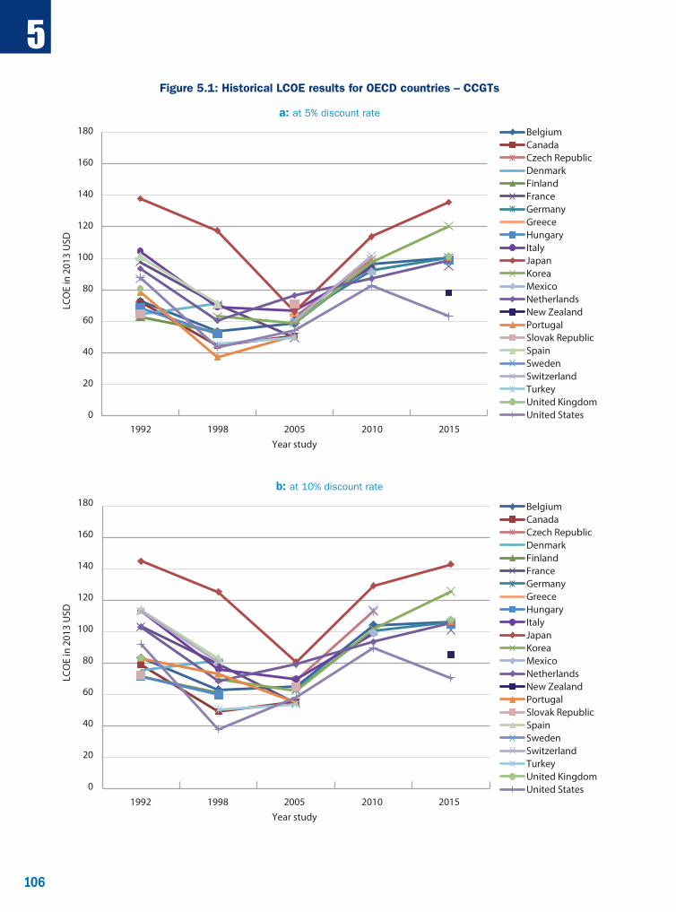
106

5

106

Figure 5.1: Historical LCOE results for OECD countries – CCGTs

a: at 5% discount rate

0

20

40

60

80

100

120

140

160

180

1992 1998 2005 2010 2015

LCO

E in

201

3 U

SD

0

20

40

60

80

100

120

140

160

180

LCO

E in

201

3 U

SD

Year study

1992 1998 2005 2010 2015Year study

BelgiumCanadaCzech RepublicDenmarkFinlandFranceGermanyGreeceHungaryItalyJapanKoreaMexicoNetherlandsNew ZealandPortugalSlovak RepublicSpainSwedenSwitzerlandTurkeyUnited KingdomUnited States

BelgiumCanadaCzech RepublicDenmarkFinlandFranceGermanyGreeceHungaryItalyJapanKoreaMexicoNetherlandsNew ZealandPortugalSlovak RepublicSpainSwedenSwitzerlandTurkeyUnited KingdomUnited States

b: at 10% discount rate

0

20

40

60

80

100

120

140

160

180

1992 1998 2005 2010 2015

LCO

E in

201

3 U

SD

0

20

40

60

80

100

120

140

160

180

LCO

E in

201

3 U

SD

Year study

1992 1998 2005 2010 2015Year study

BelgiumCanadaCzech RepublicDenmarkFinlandFranceGermanyGreeceHungaryItalyJapanKoreaMexicoNetherlandsNew ZealandPortugalSlovak RepublicSpainSwedenSwitzerlandTurkeyUnited KingdomUnited States

BelgiumCanadaCzech RepublicDenmarkFinlandFranceGermanyGreeceHungaryItalyJapanKoreaMexicoNetherlandsNew ZealandPortugalSlovak RepublicSpainSwedenSwitzerlandTurkeyUnited KingdomUnited States

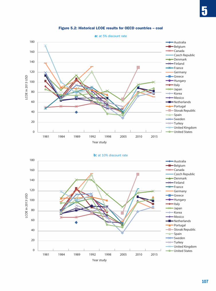
107

5

107

Figure 5.2: Historical LCOE results for OECD countries – coal

a: at 5% discount rate

0

20

40

60

80

100

120

140

160

180

1981 1984 1989 1992 1998 2005 2010 2015

LCO

E in

201

3 U

SD

0

20

40

60

80

100

120

140

160

180

LCO

E in

201

3 U

SD

Year study

1981 1984 1989 1992 1998 2005 2010 2015

Year study

AustraliaBelgiumCanadaCzech RepublicDenmarkFinlandFranceGermanyGreeceHungaryItalyJapanKoreaMexicoNetherlandsPortugalSlovak RepublicSpainSwedenTurkeyUnited KingdomUnited States

AustraliaBelgiumCanadaCzech RepublicDenmarkFinlandFranceGermanyGreeceHungaryItalyJapanKoreaMexicoNetherlandsPortugalSlovak RepublicSpainSwedenTurkeyUnited KingdomUnited States

b: at 10% discount rate

0

20

40

60

80

100

120

140

160

180

1981 1984 1989 1992 1998 2005 2010 2015

LCO

E in

201

3 U

SD

0

20

40

60

80

100

120

140

160

180

LCO

E in

201

3 U

SD

Year study

1981 1984 1989 1992 1998 2005 2010 2015

Year study

AustraliaBelgiumCanadaCzech RepublicDenmarkFinlandFranceGermanyGreeceHungaryItalyJapanKoreaMexicoNetherlandsPortugalSlovak RepublicSpainSwedenTurkeyUnited KingdomUnited States

AustraliaBelgiumCanadaCzech RepublicDenmarkFinlandFranceGermanyGreeceHungaryItalyJapanKoreaMexicoNetherlandsPortugalSlovak RepublicSpainSwedenTurkeyUnited KingdomUnited States

108

5

108

Figure 5.3: Historical LCOE results for OECD countries – nuclear

a: at 5% discount rate

1981 1984 1989 1992 1998 2005 2010 2015

Year study

1981 1984 1989 1992 1998 2005 2010 2015

Year study

0

20

40

60

80

100

120

140

160

180

LCO

E in

201

3 U

SD

0

20

40

60

80

100

120

140

160

180

LCO

E in

201

3 U

SD

BelgiumCanadaCzech RepublicFinlandFranceGermanyHungaryItalyJapanKoreaNetherlandsSlovak RepublicSpainSwitzerlandTurkeyUnited KingdomUnited States

BelgiumCanadaCzech RepublicFinlandFranceGermanyHungaryItalyJapanKoreaNetherlandsSlovak RepublicSpainSwitzerlandTurkeyUnited KingdomUnited States

b: at 10% discount rate

1981 1984 1989 1992 1998 2005 2010 2015

Year study

1981 1984 1989 1992 1998 2005 2010 2015

Year study

0

20

40

60

80

100

120

140

160

180

LCO

E in

201

3 U

SD

0

20

40

60

80

100

120

140

160

180

LCO

E in

201

3 U

SD

BelgiumCanadaCzech RepublicFinlandFranceGermanyHungaryItalyJapanKoreaNetherlandsSlovak RepublicSpainSwitzerlandTurkeyUnited KingdomUnited States

BelgiumCanadaCzech RepublicFinlandFranceGermanyHungaryItalyJapanKoreaNetherlandsSlovak RepublicSpainSwitzerlandTurkeyUnited KingdomUnited States

Part 2Statistical and sensitivity analysis

111

6

111

Chapter

Statistical analysis of key technologies

In order to examine the sensitivity of the levelised cost of electricity (LCOE) calculations to changes in underlying parameters, a set of hypothetical power plants was first developed based on the median values of the EGC 2015 dataset. Median as opposed to mean values were calculated in order to reduce the influence of outliers. The focus was on a subset of technologies (specifically, natural gas- and coal-fired generators, nuclear power plants, onshore wind, and solar photovoltaic).

It is important to note that, because specific countries and specific technologies are better represented than others, the database cannot be considered a statistical sample. Tables 6.1 through 6.7 provide the relevant statistics for each of the electricity-generating technologies in question.

In addition, Section 6.1 below presents an analysis of the solar PV LCOEs based on a weighted average analysis.

Table 6.1: Overview of data for natural gas generation

MEDIAN CASE: NATURAL GAS

(CCGT)

Net capacity (MWe)

Electrical conversion

efficiency (%)

Overnight cost

(USD/kWe)

Fixed O&M costs

(USD/MWe)

Variable O&M costs

(USD/MWh)Number of countries 12Count 13 12 13 12 11Maximum 900 61% 1 289 48 172 4.3Minimum 350 45% 627 14 667 0.2Mean 551 58% 1 021 30 568 2.5Median 475 59% 1 014 29 435 2.7Delta 550 16% 662 33 505 4.1

Table 6.2: Overview of data for coal generation

MEDIAN CASE: COAL

Net capacity (MWe)

Electrical conversion

efficiency (%)

Overnight cost

(USD/kWe)

Fixed O&M costs1

(USD/MWe)

Variable O&M costs1

(USD/MWh)Number of countries 9Count 14 14 14 14 14Maximum 4 693 51% 3 067 92 123 12.7Minimum 605 40% 813 0 0.0Mean 1 131 44% 2 080 37 818 3.8Median 772 45% 2 264 34 542 3.4Delta 4 088 11% 2 254 92 123 12.71. Zero values for fixed and variable O&M cost do not refer to the same data point.

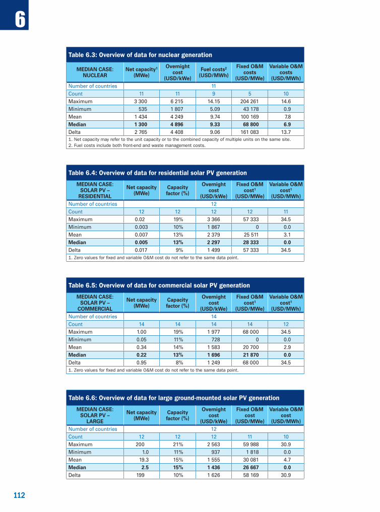
112

6

112

Table 6.3: Overview of data for nuclear generation

MEDIAN CASE: NUCLEAR

Net capacity1 (MWe)

Overnight cost

(USD/kWe)

Fuel costs2 (USD/MWh)

Fixed O&M costs

(USD/MWe)

Variable O&M costs

(USD/MWh)Number of countries 11Count 11 11 9 5 10Maximum 3 300 6 215 14.15 204 261 14.6Minimum 535 1 807 5.09 43 178 0.9Mean 1 434 4 249 9.74 100 169 7.8Median 1 300 4 896 9.33 68 800 6.9Delta 2 765 4 408 9.06 161 083 13.71. Net capacity may refer to the unit capacity or to the combined capacity of multiple units on the same site.2. Fuel costs include both front-end and waste management costs.

Table 6.4: Overview of data for residential solar PV generation

MEDIAN CASE: SOLAR PV –

RESIDENTIAL

Net capacity (MWe)

Capacity factor (%)

Overnight cost

(USD/kWe)

Fixed O&M cost1

(USD/MWe)

Variable O&M cost1

(USD/MWh)Number of countries 12Count 12 12 12 12 11Maximum 0.02 19% 3 366 57 333 34.5Minimum 0.003 10% 1 867 0 0.0Mean 0.007 13% 2 379 25 511 3.1Median 0.005 13% 2 297 28 333 0.0Delta 0.017 9% 1 499 57 333 34.51. Zero values for fixed and variable O&M cost do not refer to the same data point.

Table 6.5: Overview of data for commercial solar PV generation

MEDIAN CASE: SOLAR PV –

COMMERCIAL

Net capacity (MWe)

Capacity factor (%)

Overnight cost

(USD/kWe)

Fixed O&M cost1

(USD/MWe)

Variable O&M cost1

(USD/MWh)Number of countries 14Count 14 14 14 14 12Maximum 1.00 19% 1 977 68 000 34.5Minimum 0.05 11% 728 0 0.0Mean 0.34 14% 1 583 20 700 2.9Median 0.22 13% 1 696 21 870 0.0Delta 0.95 8% 1 249 68 000 34.51. Zero values for fixed and variable O&M cost do not refer to the same data point.

Table 6.6: Overview of data for large ground-mounted solar PV generation

MEDIAN CASE: SOLAR PV –

LARGE

Net capacity (MWe)

Capacity factor (%)

Overnight cost

(USD/kWe)

Fixed O&M cost

(USD/MWe)

Variable O&M cost

(USD/MWh)Number of countries 12Count 12 12 12 11 10Maximum 200 21% 2 563 59 988 30.9Minimum 1.0 11% 937 1 818 0.0Mean 19.3 15% 1 555 30 081 4.7Median 2.5 15% 1 436 26 667 0.0Delta 199 10% 1 626 58 169 30.9

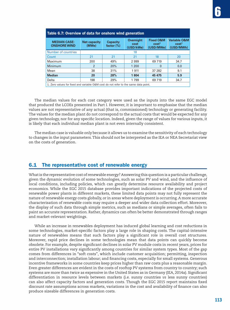
113

6

113

Table 6.7: Overview of data for onshore wind generation

MEDIAN CASE: ONSHORE WIND

Net capacity (MWe)

Capacity factor (%)

Overnight cost

(USD/kWe)

Fixed O&M cost1

(USD/MWe)

Variable O&M cost1

(USD/MWh)Number of countries 18Count 21 21 21 18 20Maximum 200 49% 2 999 69 719 34.7Minimum 2 20% 1 200 0 0.0Mean 38 31% 1 911 37 282 9.1Median 20 28% 1 804 45 475 5.9Delta 198 29% 1 799 69 719 34.71. Zero values for fixed and variable O&M cost do not refer to the same data point.

The median values for each cost category were used as the inputs into the same EGC model that produced the LCOEs presented in Part I. However, it is important to emphasise that the median values are not representative of any actual (that is, commissioned) technology or generating facility. The values for the median plant do not correspond to the actual costs that would be expected for any given technology, nor for any specific location. Indeed, given the range of values for various inputs, it is likely that each individual median plant is not even internally consistent.

The median case is valuable only because it allows us to examine the sensitivity of each technology to changes in the input parameters. This should not be interpreted as the IEA or NEA Secretariat view on the costs of generation.

6.1 The representative cost of renewable energy

What is the representative cost of renewable energy? Answering this question is a particular challenge, given the dynamic evolution of some technologies, such as solar PV and wind, and the influence of local conditions, including policies, which can greatly determine resource availability and project economics. While the EGC 2015 database provides important indications of the projected costs of renewable power plants in different markets, these limited data points may not fully represent the nature of renewable energy costs globally, or in areas where deployment is occurring. A more accurate characterisation of renewable costs may require a deeper and wider data collection effort. Moreover, the display of such data through simple metrics, such as medians or simple averages, often fails to paint an accurate representation. Rather, dynamics can often be better demonstrated through ranges and market-relevant weightings.

While an increase in renewables deployment has induced global learning and cost reductions in some technologies, market-specific factors play a large role in shaping costs. The capital-intensive nature of renewables means that such factors play a significant role in overall cost structures. Moreover, rapid price declines in some technologies mean that data points can quickly become obsolete. For example, despite significant declines in solar PV module costs in recent years, prices for entire PV installations vary significantly among countries for similar system types. Most of the gap comes from differences in “soft costs”, which include customer acquisition; permitting, inspection and interconnection; installation labour; and financing costs, especially for small systems. Generous incentive frameworks in some countries keep prices higher than raw costs plus a reasonable margin. Even greater differences are evident in the costs of rooftop PV systems from country to country; such systems are more than twice as expensive in the United States as in Germany (IEA, 2014a). Significant differentiation in resource levels between markets (i.e. sunny countries vs less sunny countries) can also affect capacity factors and generation costs. Though the EGC 2015 report maintains fixed discount rate assumptions across markets, variations in the cost and availability of finance can also produce sizeable differences in generation costs.

114

6

114

The EGC 2015 database reflects a wide range of overnight costs and capacity factors for solar PV across the residential, commercial and large, ground-mounted segments. However, given the limited country and plant sample sizes (11 to 13 plants, depending on segment), it can be difficult to evaluate the representativeness of these datapoints in the wider context of solar PV deployment. Metrics such as medians or simple averages can be misleading because they give equal weight to markets or plants that may be less relevant for global PV deployment. Another study, by the International Renewable Energy Agency (IRENA) on Renewable Power Generation Costs in 2014, presents a much larger project-level dataset that is continually updated, with segment ranges and capacity-weighted average levelised costs calculated by region (IRENA, 2014). Such a sample size and corresponding metrics give a broader indication of the diversity of costs for solar PV projects because of local conditions, and also identify the most representative cost structures as a function of where capacity is most deployed (Figure 6.1).

Figure 6.1: LCOEs for utility-scale solar PV, by project, 2013 and 2014

2014 USD/kWh

Capacity MWe

1

100

200

> 300

0.5

0.4

0.3

0.2

0.1

0.0

Africa China Europe Central andSouth America

MiddleEast

NorthAmerica

Oceania OtherAsia

Source: IRENA Renewable Cost Database and Photon Consulting, 2014.

115

6

115

One way to better represent the market dynamics of solar PV using EGC 2015 data is to weight the cost results according to the expected top solar PV markets (e.g. China, the United States, Japan) in 2020. Taking a weighted average of solar PV LCOEs produces a lower overall cost compared to simple averages and medians, but this result better represents expected market dynamics. The Medium-term Renewable Energy Market Report (IEA, 2014b), or the MTRMR, goes one step forward towards displaying more representative costs. Though not a cost study per se, the MTRMR tries to identify the most dynamic markets for solar PV deployment over the medium term and focuses cost evaluation efforts on these areas (IEA, 2014b). Unlike EGC 2015, the MTRMR also tries to apply market-specific discount rates to its LCOE calculations, though such values can carry a degree of uncertainty. The upshot of such an approach is that the MTRMR cost analysis better reflects the expected trend of deployment – that capacity installations continue to move from historical growth markets in Europe to expanding markets in Asia and the Americas, where solar resources are generally better.1

Figure 6.2: Utility-scale solar PV LCOEs projected in 2020

USD

/MW

h

AverageMedian Weighted average – based on MTRMR generation forecast in 2020

0

25

50

75

100

125

150

175

200

MTRMR 2014 sample*EGC – 10% WACCEGC – 7% WACCEGC – 3% WACC

* Note: EGC country sample includes Belgium, China, Denmark, France, Germany, Hungary, Italy, Japan, Korea, Spain, the United Kingdom and the United States.

References

IEA (2014a), Technology Roadmap: Solar Photovoltaic Energy, OECD, Paris.

IEA (2014b), Medium-term Renewable Energy Market Report, OECD, Paris.

IRENA (2015), Renewable Power Generation Costs in 2014, International Renewable Energy Agency, Abu Dhabi.

1. MTRMR (IEA, 2014) weighted average weights forecasted typical LCOEs across key PV deployment markets (Australia, Brazil, China, France, Germany, India, Italy, Japan, Korea, Mexico, South Africa, the United Arab Emirates, the United Kingdom and the United States) according to the additions they expect from new PV generation in 2020. Weighted average cost of capital (WACC) is not uniform and varies according to country-level assumptions.

117

7

117

Chapter

Sensitivity analysis

This chapter continues the analysis first performed in EGC 2010, examining the sensitivity of the levelised cost of electricity (LCOE) calculated for a particular set of generation types to variations in the underlying parameters. By necessity, the EGC reports must make a set of simplifying assumptions when performing the cost analysis – assuming a constant capacity factor, for example, or fuel price. In reality, the input parameters will vary across – or even within – countries.

We use a hypothetical median power plant, drawn from inputs developed in Chapter 6, as the basis for this analysis.

Section 7.1 presents a technology-specific analysis of the influence on LCOE of a ±50% change in each key parameter. Section 7.2 compares the relative sensitivity of the various technologies to each other as specific inputs are adjusted.

7.1 Multidimensional sensitivity analysis

This section presents the sensitivity of the LCOE for each of the main technologies to changes in the underlying input parameters. Specifically, the median value of each input into the LCOE calculation1 is adjusted by ±50% and evaluate the impact. Each parameter is adjusted independently of the others, so as to isolate the influence of each change on the final result, and presented as “tornado charts” so that the relative impact of each change can be compared.

1. Specifically, discount rate, overnight cost, lifetime, fuel cost, carbon cost, and construction lead time; for renewable technologies, the capacity factor is also adjusted.

118

7

118

For each of the following charts, the vertical axis indicates the median case LCOE value, while the horizontal bars present the increase or decrease in LCOE (in percentage terms) after the parameter has been adjusted by ±50%. This is done separately for each of the three discount rates used in the core analysis (3%, 7% and 10%).2 Figure 7.1 shows the results of this analysis for combined-cycle gas turbines (CCGTs).

Figure 7.1: Tornado charts – natural gas (CCGT)

-60 -40 -20 0 20 40 60

Lead time

Carbon cost

Fuel cost

Lifetime

Overnight cost

Discount rate

-60 -40 -20 0 20 40 60 -60 -40 -20 0 20 40 60

Impact on LCOE Impact on LCOE Impact on LCOE

Median case (at 3% discount rate)

Median case (at 7% discount rate)

Median case (at 10% discount rate)

%

The single largest factor influencing the LCOE of natural gas plants is fuel cost. At a 3% discount rate, carbon costs are the second most important factor, though at higher discount rates, overnight cost is more significant. Not surprisingly, the influence of changes in the discount rate is more pronounced the higher the median-case discount rate is, as a 50% change in a 10% discount rate is larger, in absolute terms, than a 50% change in a 3% discount rate.

Lifetime is inversely correlated with LCOE, so the increase in LCOE is associated with a decrease in lifetime. In this case, an early retirement has a more significant impact on the LCOE than a lifetime extension.

2. For example, the discount rate is adjusted by 50% relative to the starting point, i.e. the 3% discount rate is changed to 1.5% and 4.5%, while the 10% rate is changed to 5% and 15%.

119

7

119

Figure 7.2 show the results of the same analysis for a coal plant.

Figure 7.2: Tornado charts – coal

-60 -40 -20 0 20 40 60

Lead time

Carbon cost

Fuel cost

Lifetime

Overnight cost

Discount rate

-60 -40 -20 0 20 40 60 -60 -40 -20 0 20 40 60

Impact on LCOE Impact on LCOE Impact on LCOE

Median case (at 3% discount rate)

Median case (at 7% discount rate)

Median case (at 10% discount rate)

%

The impacts of cost drivers for coal plant costs are more uniform, in particular at higher discount rates. Fuel cost is the most important factor at 3% and 5% discount rates, whereas a 50% change in the discount rate has the most significant impact when the discount rate is initially 10%, followed closely by overnight cost. The carbon cost impact is quite important at all discount rates. Coal plant costs are also more sensitive to early retirement than natural gas plants – and, conversely, they derive slightly more benefit from lifetime extensions.

Figure 7.3 shows the results of this analysis for a nuclear plant.

Figure 7.3: Tornado charts – nuclear

-60 -40 -20 0 20 40 60

Lead time

Carbon cost

Fuel cost

Lifetime

Overnight cost

Discount rate

-60 -40 -20 0 20 40 60 -60 -40 -20 0 20 40 60

Impact on LCOE Impact on LCOE Impact on LCOE

Median case (at 3% discount rate)

Median case (at 7% discount rate)

Median case (at 10% discount rate)

%

120

7

120

The cost of nuclear plants is largely driven by the overnight cost. At a 3% discount rate, overnight cost is the dominant input, closely followed by the discount rate. Changes in the discount rate are more important at the 5% and 10% starting points, though changes in overnight costs also have a large influence on LCOE at those rates. The impact of changes in construction lead time gives some sense as to why this is the case. Nuclear plants have long construction times, and so costs are highly sensitive to delays in construction or to changes in the discount rate. Changes in lifetime are far more important at low discount rates than at high rates. Fuel costs, on the other hand, are a relatively small component of the final LCOE, and so variations in these costs have less of an influence.

Figure 7.4 shows the results of the analysis for a solar PV plant. While Chapter 6 presents the median inputs for all three categories of solar PV (residential rooftop, commercial rooftop, and large ground-mounted), the differences in sensitivity to input changes are relatively small across categories. The analysis is therefore only presented for commercial rooftop solar PV.

Figure 7.4: Tornado charts – solar PV, commercial rooftop

-60 -40 -20 0 20 40 60 80 100

Lead time

Carbon cost

Fuel cost

Lifetime

Overnight cost

Discount rate

Capacity factor

-60 -40 -20 0 20 40 60 80 100 -60 -40 -20 0 20 40 60 80 100

Impact on LCOE Impact on LCOE Impact on LCOE

Median case (at 3% discount rate)

Median case (at 7% discount rate)

Median case (at 10% discount rate)

%

For solar PV (and onshore wind below) an additional sensitivity on the capacity factor is added. Here the capacity factor is the dominant factor in determining the final LCOE, followed by lifetime. The capacity factor in this case is also inversely correlated to LCOE, with higher capacity factors resulting in lower LCOEs. Lifetime is of particular importance at all discount rates.

121

7

121

Figure 7.5 shows the results for onshore wind.

Figure 7.5: Tornado charts – onshore wind

-60 -40 -20 0 20 40 60 80 100

Lead time

Carbon cost

Fuel cost

Lifetime

Overnight cost

Discount rate

Capacity factor

-60 -40 -20 0 20 40 60 80 100 -60 -40 -20 0 20 40 60 80 100

Impact on LCOE Impact on LCOE Impact on LCOE

Median case (at 3% discount rate)

Median case (at 7% discount rate)

Median case (at 10% discount rate)

%

The cost of onshore wind shows more dependence on the various impacts than solar PV, with the capacity factor being the most important factor. Changes in overnight costs and lifetime, however, are more significant for this technology compared to solar PV at all discount rates. The relatively short construction time for this technology, however, means that it is relatively insensitive to delays (or improvements) in construction lead time.

7.2 Detailed sensitivity analysis

The following subsections present the sensitivity of each technology to a range of values for each input parameter. Here different technologies are compared, while focusing on a particular input parameter. Doing so provides a benchmark for understanding the relative sensitivity of each technology to different market conditions (for example changes in fuel prices) or different development conditions (for example changes in construction lead time).

This analysis closely follows the analysis performed in EGC 2010, offering an opportunity to compare these updated results to the previous analysis to check the consistency of the updated data with the prior dataset and examine changes in the sensitivities. All values are normalised, with 100 representing the reference point for each technology.3

3. In general, this is the median case LCOE, though it will vary depending on the analysis in question.

122

7

122

Discount rate sensitivity

Changes in discount rates affect each technology across a number of dimensions, such as overnight costs, construction lead times, and lifespan. Broadly speaking, however, the more capital-intensive a technology is, the more sensitive it is to changes in the discount rate. This is illustrated clearly in Figure 7.6, where the discount rate is adjusted from a low of 0% to a high of 15%.

Figure 7.6: LCOE as a function of the discount rate

Onshore windCoal Nuclear Solar PVCCGT

% o

f med

ian

LCO

E

Discount rate

0

50

100

150

200

250

300

350

400

450

500

15%14%13%12%11%10%9%8%7%6%5%4%3%2%1%0%

The technology least sensitive to discount rates is natural gas-fired CCGTs, which sees only a 24% increase in LCOE as the discount rate is increased from 0% to 15%, followed by coal-fired generation, which increases by 71%. Both of these technologies have relatively low upfront costs relative to their variable costs, in particular fuel costs.

Nuclear power, on the other hand, is the most sensitive to changes in the discount rate, with its LCOE increasing by 349% over that same range. This is mainly because nuclear power has a significantly longer construction lead time than other technologies, though higher discount rates do also diminish the benefits that nuclear plants receive from their relatively longer lifespans.

Along similar lines, the influence of changing the discount rate on the capital intensity of the technology was analysed – that is, the ratio of the technology’s levelised investment cost to its total levelised cost. The capital intensity of a technology is important because it is an indicator of how highly sensitive it is to market prices. Technologies that are more capital-intensive will require higher prices, or longer periods over which to earn revenues, in order to recover the upfront investment cost. On the other hand, these technologies are less sensitive to changes that affect variable costs, such as fuel prices. For this reason, capital-intensive technologies are more sensitive to volatile electricity prices, and are therefore more likely to seek long-term guaranteed revenues in the form of power purchase agreements or feed-in tariffs.

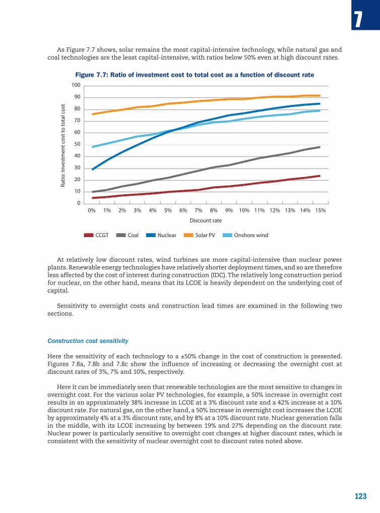
123

7

123

As Figure 7.7 shows, solar remains the most capital-intensive technology, while natural gas and coal technologies are the least capital-intensive, with ratios below 50% even at high discount rates.

Figure 7.7: Ratio of investment cost to total cost as a function of discount rate

Onshore windCoal Nuclear Solar PVCCGT

Ratio

: inv

estm

ent c

ost t

o to

tal c

ost

Discount rate

0

10

20

30

40

50

60

70

80

90

100

15%14%13%12%11%10%9%8%7%6%5%4%3%2%1%0%

At relatively low discount rates, wind turbines are more capital-intensive than nuclear power plants. Renewable energy technologies have relatively shorter deployment times, and so are therefore less affected by the cost of interest during construction (IDC). The relatively long construction period for nuclear, on the other hand, means that its LCOE is heavily dependent on the underlying cost of capital.

Sensitivity to overnight costs and construction lead times are examined in the following two sections.

Construction cost sensitivity

Here the sensitivity of each technology to a ±50% change in the cost of construction is presented. Figures 7.8a, 7.8b and 7.8c show the influence of increasing or decreasing the overnight cost at discount rates of 3%, 7% and 10%, respectively.

Here it can be immediately seen that renewable technologies are the most sensitive to changes in overnight cost. For the various solar PV technologies, for example, a 50% increase in overnight cost results in an approximately 38% increase in LCOE at a 3% discount rate and a 42% increase at a 10% discount rate. For natural gas, on the other hand, a 50% increase in overnight cost increases the LCOE by approximately 4% at a 3% discount rate, and by 8% at a 10% discount rate. Nuclear generation falls in the middle, with its LCOE increasing by between 19% and 27% depending on the discount rate. Nuclear power is particularly sensitive to overnight cost changes at higher discount rates, which is consistent with the sensitivity of nuclear overnight cost to discount rates noted above.

124

7

124

Figure 7.8: LCOE as a function of overnight cost

a: at 3% discount rate

% o

f med

ian

case

LCO

E

Onshore windCoal Nuclear Solar PVCCGT

50

60

70

80

90

100

110

120

130

140

150

+50%+40%+30%+20%+10%Mediancase

-10%-20%-30%-40%-50%

% o

f med

ian

case

LCO

E

Onshore windCoal Nuclear Solar PVCCGT

50

60

70

80

90

100

110

120

130

140

150

+50%+40%+30%+20%+10%Mediancase

-10%-20%-30%-40%-50%

% o

f med

ian

case

LCO

E

Onshore windCoal Nuclear Solar PVCCGT

50

60

70

80

90

100

110

120

130

140

150

+50%+40%+30%+20%+10%Mediancase

-10%-20%-30%-40%-50%

b: at 7% discount rate

% o

f med

ian

case

LCO

E

Onshore windCoal Nuclear Solar PVCCGT

50

60

70

80

90

100

110

120

130

140

150

+50%+40%+30%+20%+10%Mediancase

-10%-20%-30%-40%-50%

% o

f med

ian

case

LCO

E

Onshore windCoal Nuclear Solar PVCCGT

50

60

70

80

90

100

110

120

130

140

150

+50%+40%+30%+20%+10%Mediancase

-10%-20%-30%-40%-50%

% o

f med

ian

case

LCO

E

Onshore windCoal Nuclear Solar PVCCGT

50

60

70

80

90

100

110

120

130

140

150

+50%+40%+30%+20%+10%Mediancase

-10%-20%-30%-40%-50%

c: at 10% discount rate

% o

f med

ian

case

LCO

E

Onshore windCoal Nuclear Solar PVCCGT

50

60

70

80

90

100

110

120

130

140

150

+50%+40%+30%+20%+10%Mediancase

-10%-20%-30%-40%-50%

% o

f med

ian

case

LCO

E

Onshore windCoal Nuclear Solar PVCCGT

50

60

70

80

90

100

110

120

130

140

150

+50%+40%+30%+20%+10%Mediancase

-10%-20%-30%-40%-50%

% o

f med

ian

case

LCO

E

Onshore windCoal Nuclear Solar PVCCGT

50

60

70

80

90

100

110

120

130

140

150

+50%+40%+30%+20%+10%Mediancase

-10%-20%-30%-40%-50%

125

7

125

Construction lead time sensitivity

Construction lead time can have a significant influence on LCOE, in particular at higher discount rates. The construction period, for the purpose of this report, is defined to be the length of time from the first pouring of concrete until the commissioning date (here assumed to be 2020 for all technologies).

In this section, the influence of increasing the construction period by up to five years at each of the three discount rates is examined. This analysis takes the unrealistic assumption that increases in construction lead times do not occur with an associated increase in investment cost. For an actual plant, any increase in the construction period would be associated with some increase in overnight cost that go beyond the costs associated with IDC. It is also assumed that overnight costs are spread evenly throughout the construction period. For some technologies – in particular nuclear – this may not be the case, and so the influence of construction delays on LCOE would be lower than what this analysis suggests.

Figure 7.9: LCOE as a function of construction lead time

a: at 3% discount rate

% o

f med

ian

case

LCO

E

Onshore windCoal Nuclear Solar PVCCGT

90

95

100

105

110

115

120

125

130

+5 year+4 year+3 year+2 year+1 yearMedian case

% o

f med

ian

case

LCO

E

Onshore windCoal Nuclear Solar PVCCGT

90

95

100

105

110

115

120

125

130

+5 year+4 year+3 year+2 year+1 yearMedian case

% o

f med

ian

case

LCO

E

Onshore windCoal Nuclear Solar PVCCGT

90

95

100

105

110

115

120

125

130

+5 year+4 year+3 year+2 year+1 yearMedian case

b: at 7% discount rate

% o

f med

ian

case

LCO

E

Onshore windCoal Nuclear Solar PVCCGT

90

95

100

105

110

115

120

125

130

+5 year+4 year+3 year+2 year+1 yearMedian case

% o

f med

ian

case

LCO

E

Onshore windCoal Nuclear Solar PVCCGT

90

95

100

105

110

115

120

125

130

+5 year+4 year+3 year+2 year+1 yearMedian case

% o

f med

ian

case

LCO

E

Onshore windCoal Nuclear Solar PVCCGT

90

95

100

105

110

115

120

125

130

+5 year+4 year+3 year+2 year+1 yearMedian case

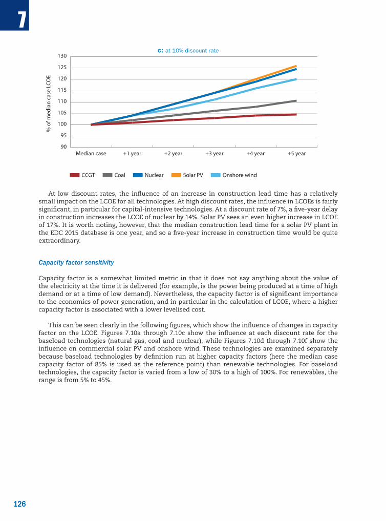
126

7

126

c: at 10% discount rate%

of m

edia

n ca

se L

COE

Onshore windCoal Nuclear Solar PVCCGT

90

95

100

105

110

115

120

125

130

+5 year+4 year+3 year+2 year+1 yearMedian case

% o

f med

ian

case

LCO

E

Onshore windCoal Nuclear Solar PVCCGT

90

95

100

105

110

115

120

125

130

+5 year+4 year+3 year+2 year+1 yearMedian case

% o

f med

ian

case

LCO

E

Onshore windCoal Nuclear Solar PVCCGT

90

95

100

105

110

115

120

125

130

+5 year+4 year+3 year+2 year+1 yearMedian case

At low discount rates, the influence of an increase in construction lead time has a relatively small impact on the LCOE for all technologies. At high discount rates, the influence in LCOEs is fairly significant, in particular for capital-intensive technologies. At a discount rate of 7%, a five-year delay in construction increases the LCOE of nuclear by 14%. Solar PV sees an even higher increase in LCOE of 17%. It is worth noting, however, that the median construction lead time for a solar PV plant in the EDC 2015 database is one year, and so a five-year increase in construction time would be quite extraordinary.

Capacity factor sensitivity

Capacity factor is a somewhat limited metric in that it does not say anything about the value of the electricity at the time it is delivered (for example, is the power being produced at a time of high demand or at a time of low demand). Nevertheless, the capacity factor is of significant importance to the economics of power generation, and in particular in the calculation of LCOE, where a higher capacity factor is associated with a lower levelised cost.

This can be seen clearly in the following figures, which show the influence of changes in capacity factor on the LCOE. Figures 7.10a through 7.10c show the influence at each discount rate for the baseload technologies (natural gas, coal and nuclear), while Figures 7.10d through 7.10f show the influence on commercial solar PV and onshore wind. These technologies are examined separately because baseload technologies by definition run at higher capacity factors (here the median case capacity factor of 85% is used as the reference point) than renewable technologies. For baseload technologies, the capacity factor is varied from a low of 30% to a high of 100%. For renewables, the range is from 5% to 45%.

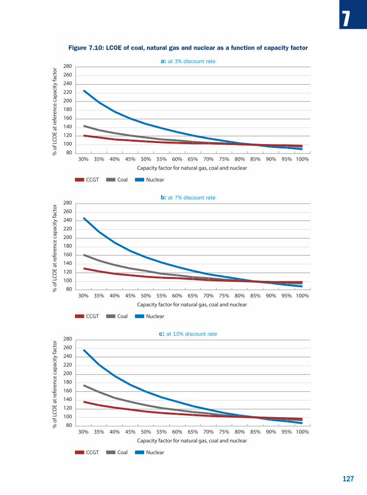
127

7

127

Figure 7.10: LCOE of coal, natural gas and nuclear as a function of capacity factor

a: at 3% discount rate%

of L

COE

at re

fere

nce

capa

city

fact

or

Coal NuclearCCGT

80

100

120

140

160

180

200

220

240

260

280

100%95%90%85%80%75%70%65%60%55%50%45%40%35%30%

Capacity factor for natural gas, coal and nuclear

% o

f LCO

E at

refe

renc

e ca

paci

ty fa

ctor

Coal NuclearCCGT

80

100

120

140

160

180

200

220

240

260

280

100%95%90%85%80%75%70%65%60%55%50%45%40%35%30%

Capacity factor for natural gas, coal and nuclear

% o

f LCO

E at

refe

renc

e ca

paci

ty fa

ctor

Coal NuclearCCGT

80

100

120

140

160

180

200

220

240

260

280

100%95%90%85%80%75%70%65%60%55%50%45%40%35%30%

Capacity factor for natural gas, coal and nuclear

b: at 7% discount rate

% o

f LCO

E at

refe

renc

e ca

paci

ty fa

ctor

Coal NuclearCCGT

80

100

120

140

160

180

200

220

240

260

280

100%95%90%85%80%75%70%65%60%55%50%45%40%35%30%

Capacity factor for natural gas, coal and nuclear

% o

f LCO

E at

refe

renc

e ca

paci

ty fa

ctor

Coal NuclearCCGT

80

100

120

140

160

180

200

220

240

260

280

100%95%90%85%80%75%70%65%60%55%50%45%40%35%30%

Capacity factor for natural gas, coal and nuclear

% o

f LCO

E at

refe

renc

e ca

paci

ty fa

ctor

Coal NuclearCCGT

80

100

120

140

160

180

200

220

240

260

280

100%95%90%85%80%75%70%65%60%55%50%45%40%35%30%

Capacity factor for natural gas, coal and nuclear

c: at 10% discount rate

% o

f LCO

E at

refe

renc

e ca

paci

ty fa

ctor

Coal NuclearCCGT

80

100

120

140

160

180

200

220

240

260

280

100%95%90%85%80%75%70%65%60%55%50%45%40%35%30%

Capacity factor for natural gas, coal and nuclear

% o

f LCO

E at

refe

renc

e ca

paci

ty fa

ctor

Coal NuclearCCGT

80

100

120

140

160

180

200

220

240

260

280

100%95%90%85%80%75%70%65%60%55%50%45%40%35%30%

Capacity factor for natural gas, coal and nuclear

% o

f LCO

E at

refe

renc

e ca

paci

ty fa

ctor

Coal NuclearCCGT

80

100

120

140

160

180

200

220

240

260

280

100%95%90%85%80%75%70%65%60%55%50%45%40%35%30%

Capacity factor for natural gas, coal and nuclear

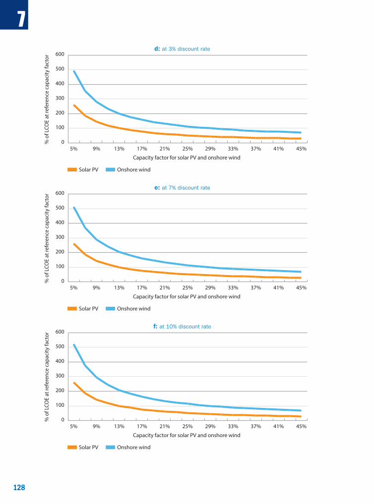
128

7

128

d: at 3% discount rate

0

100

200

300

400

500

600

45%41%37%33%29%25%21%17%13%9%5%

% o

f LCO

E at

refe

renc

e ca

paci

ty fa

ctor

Capacity factor for solar PV and onshore wind

0

100

200

300

400

500

600

45%41%37%33%29%25%21%17%13%9%5%

% o

f LCO

E at

refe

renc

e ca

paci

ty fa

ctor

Capacity factor for solar PV and onshore wind

0

100

200

300

400

500

600

45%41%37%33%29%25%21%17%13%9%5%

% o

f LCO

E at

refe

renc

e ca

paci

ty fa

ctor

Capacity factor for solar PV and onshore wind

Onshore windSolar PV

Onshore windSolar PV

Onshore windSolar PV

e: at 7% discount rate

0

100

200

300

400

500

600

45%41%37%33%29%25%21%17%13%9%5%

% o

f LCO

E at

refe

renc

e ca

paci

ty fa

ctor

Capacity factor for solar PV and onshore wind

0

100

200

300

400

500

600

45%41%37%33%29%25%21%17%13%9%5%

% o

f LCO

E at

refe

renc

e ca

paci

ty fa

ctor

Capacity factor for solar PV and onshore wind

0

100

200

300

400

500

600

45%41%37%33%29%25%21%17%13%9%5%

% o

f LCO

E at

refe

renc

e ca

paci

ty fa

ctor

Capacity factor for solar PV and onshore wind

Onshore windSolar PV

Onshore windSolar PV

Onshore windSolar PV

f: at 10% discount rate

0

100

200

300

400

500

600

45%41%37%33%29%25%21%17%13%9%5%

% o

f LCO

E at

refe

renc

e ca

paci

ty fa

ctor

Capacity factor for solar PV and onshore wind

0

100

200

300

400

500

600

45%41%37%33%29%25%21%17%13%9%5%

% o

f LCO

E at

refe

renc

e ca

paci

ty fa

ctor

Capacity factor for solar PV and onshore wind

0

100

200

300

400

500

600

45%41%37%33%29%25%21%17%13%9%5%

% o

f LCO

E at

refe

renc

e ca

paci

ty fa

ctor

Capacity factor for solar PV and onshore wind

Onshore windSolar PV

Onshore windSolar PV

Onshore windSolar PV

129

7

129

Among baseload technologies, it is immediately clear that nuclear is the most sensitive to changes in capacity factor. At a 7% discount rate, decreasing the capacity factor from 85% to 30% increases the LCOE for nuclear by 147%. This is not to imply that such capacity factors for nuclear plants are realistic. What it does reveal, however, is that the economics of nuclear power is more significantly challenged in an environment where capacity factors are diminishing than either coal or natural gas generation. Nuclear power has relatively high fixed costs, and a lower capacity factor means it has fewer hours over the course of a year over which to recover those costs. Natural gas-fired power generation, which has relatively low fixed costs, is the least influenced by lower capacity factors, increasing by only 30% at a 30% capacity factor.

Wind and solar generation plants have an even higher share of fixed costs than nuclear plants. In addition, the output from these generators is variable, and confined to a more limited time frame (in particular for solar PV, which in the absence of storage can only produce power when the sun is shining).

Lifetime sensitivity

This sensitivity varies the lifetime that each plant operates by ±25% and ±50%, with a decrease in lifetime equivalent to an early retirement, and an increase in lifetime equivalent to a no-cost lifetime extension. Each generating technology has a different expected lifetime, and for the median case the default values of 60 years for nuclear, 40 years for coal, 30 years for natural gas, and 25 years for onshore and solar PV are used.

Figure 7.11: LCOE as a function of lifetime

a: at 3% discount rate

% o

f med

ian

case

LCO

E

Onshore windCoal Nuclear Solar PVCCGT

Onshore windCoal Nuclear Solar PVCCGT

Onshore windCoal Nuclear Solar PVCCGT

80

90

100

110

120

130

140

150

160

+50%+25%Median case-25%-50%

% o

f med

ian

case

LCO

E

80

90

100

110

120

130

140

150

160

+50%+25%Median case-25%-50%

% o

f med

ian

case

LCO

E

80

90

100

110

120

130

140

150

160

+50%+25%Median case-25%-50%

b: at 7% discount rate

% o

f med

ian

case

LCO

E

Onshore windCoal Nuclear Solar PVCCGT

Onshore windCoal Nuclear Solar PVCCGT

Onshore windCoal Nuclear Solar PVCCGT

80

90

100

110

120

130

140

150

160

+50%+25%Median case-25%-50%

% o

f med

ian

case

LCO

E

80

90

100

110

120

130

140

150

160

+50%+25%Median case-25%-50%

% o

f med

ian

case

LCO

E

80

90

100

110

120

130

140

150

160

+50%+25%Median case-25%-50%

130

7

130

c: at 10% discount rate%

of m

edia

n ca

se L

COE

Onshore windCoal Nuclear Solar PVCCGT

Onshore windCoal Nuclear Solar PVCCGT

Onshore windCoal Nuclear Solar PVCCGT

80

90

100

110

120

130

140

150

160

+50%+25%Median case-25%-50%

% o

f med

ian

case

LCO

E

80

90

100

110

120

130

140

150

160

+50%+25%Median case-25%-50%

% o

f med

ian

case

LCO

E

80

90

100

110

120

130

140

150

160

+50%+25%Median case-25%-50%

It is to be noted first that a decrease in lifetime has a more significant influence on LCOE than an increase in lifetime. This is in particular the case for technologies with shorter lifespans, namely solar and wind. Most of the investment expenses are incurred early in the plants’ lifespan, and so a decrease in the overall lifetime means it has fewer years over which to recover the majority of its costs. Technologies like natural gas and coal, which are relatively less capital-intensive and which are more sensitive to fuel costs (which are incurred over the life of the plant) see a relatively smaller influence on their LCOEs.

Fuel cost sensitivity

The fuel cost sensitivity by necessity focuses on a narrower set of technologies – that is, technologies that consume fuel as part of the generating process; in this case, nuclear, coal and natural gas. Fuel prices, especially for natural gas and coal, are highly dependent on whether the technology is located in an importing or exporting country, and on global fuel markets more broadly. Because these are median-case power plants, and therefore not meant to represent the cost of these technologies in any particular county, the import costs in OECD are used for both of these, derived from the World Energy Outlook (WEO) 2014 fuel price assumptions. For nuclear power, the default assumption of USD 7/MWh is taken.4

Figures 7.12a, 7.12b and 7.12c show the influence of a ±50% change in fuel prices on the LCOE for each technology.

4. Note that, in the particular case of nuclear, there are also costs associated with waste management (here assumed to be the default value of USD 2.33/MWh). As this only affects nuclear power, and at any rate represents only a small fraction of the overall LCOE, a sensitivity on waste management costs is not included.

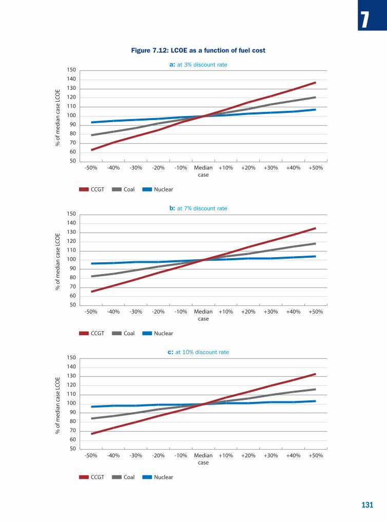
131

7

131

Figure 7.12: LCOE as a function of fuel cost

a: at 3% discount rate%

of m

edia

n ca

se L

COE

Coal NuclearCCGT

50

60

70

80

90

100

110

120

130

140

150

+50%+40%+30%+20%+10%Mediancase

-10%-20%-30%-40%-50%

% o

f med

ian

case

LCO

E

Coal NuclearCCGT

50

60

70

80

90

100

110

120

130

140

150

+50%+40%+30%+20%+10%Mediancase

-10%-20%-30%-40%-50%

% o

f med

ian

case

LCO

E

Coal NuclearCCGT

50

60

70

80

90

100

110

120

130

140

150

+50%+40%+30%+20%+10%Mediancase

-10%-20%-30%-40%-50%

b: at 7% discount rate

% o

f med

ian

case

LCO

E

Coal NuclearCCGT

50

60

70

80

90

100

110

120

130

140

150

+50%+40%+30%+20%+10%Mediancase

-10%-20%-30%-40%-50%

% o

f med

ian

case

LCO

E

Coal NuclearCCGT

50

60

70

80

90

100

110

120

130

140

150

+50%+40%+30%+20%+10%Mediancase

-10%-20%-30%-40%-50%

% o

f med

ian

case

LCO

E

Coal NuclearCCGT

50

60

70

80

90

100

110

120

130

140

150

+50%+40%+30%+20%+10%Mediancase

-10%-20%-30%-40%-50%

c: at 10% discount rate

% o

f med

ian

case

LCO

E

Coal NuclearCCGT

50

60

70

80

90

100

110

120

130

140

150

+50%+40%+30%+20%+10%Mediancase

-10%-20%-30%-40%-50%

% o

f med

ian

case

LCO

E

Coal NuclearCCGT

50

60

70

80

90

100

110

120

130

140

150

+50%+40%+30%+20%+10%Mediancase

-10%-20%-30%-40%-50%

% o

f med

ian

case

LCO

E

Coal NuclearCCGT

50

60

70

80

90

100

110

120

130

140

150

+50%+40%+30%+20%+10%Mediancase

-10%-20%-30%-40%-50%

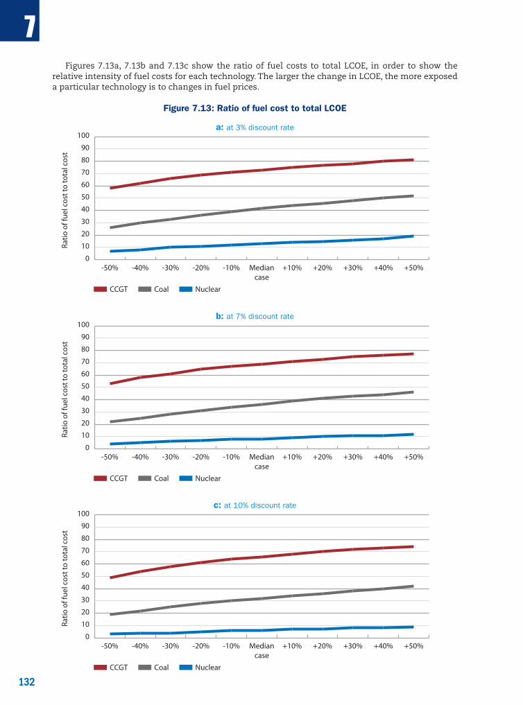
132

7

132

Figures 7.13a, 7.13b and 7.13c show the ratio of fuel costs to total LCOE, in order to show the relative intensity of fuel costs for each technology. The larger the change in LCOE, the more exposed a particular technology is to changes in fuel prices.

Figure 7.13: Ratio of fuel cost to total LCOE

a: at 3% discount rate

Ratio

of f

uel c

ost t

o to

tal c

ost

Coal NuclearCCGT

0

10

20

30

40

50

60

70

80

90

100

+50%+40%+30%+20%+10%Mediancase

-10%-20%-30%-40%-50%

Ratio

of f

uel c

ost t

o to

tal c

ost

Coal NuclearCCGT

0

10

20

30

40

50

60

70

80

90

100

+50%+40%+30%+20%+10%Mediancase

-10%-20%-30%-40%-50%

Ratio

of f

uel c

ost t

o to

tal c

ost

Coal NuclearCCGT

0

10

20

30

40

50

60

70

80

90

100

+50%+40%+30%+20%+10%Mediancase

-10%-20%-30%-40%-50%

b: at 7% discount rate

Ratio

of f

uel c

ost t

o to

tal c

ost

Coal NuclearCCGT

0

10

20

30

40

50

60

70

80

90

100

+50%+40%+30%+20%+10%Mediancase

-10%-20%-30%-40%-50%

Ratio

of f

uel c

ost t

o to

tal c

ost

Coal NuclearCCGT

0

10

20

30

40

50

60

70

80

90

100

+50%+40%+30%+20%+10%Mediancase

-10%-20%-30%-40%-50%

Ratio

of f

uel c

ost t

o to

tal c

ost

Coal NuclearCCGT

0

10

20

30

40

50

60

70

80

90

100

+50%+40%+30%+20%+10%Mediancase

-10%-20%-30%-40%-50%

c: at 10% discount rate

Ratio

of f

uel c

ost t

o to

tal c

ost

Coal NuclearCCGT

0

10

20

30

40

50

60

70

80

90

100

+50%+40%+30%+20%+10%Mediancase

-10%-20%-30%-40%-50%

Ratio

of f

uel c

ost t

o to

tal c

ost

Coal NuclearCCGT

0

10

20

30

40

50

60

70

80

90

100

+50%+40%+30%+20%+10%Mediancase

-10%-20%-30%-40%-50%

Ratio

of f

uel c

ost t

o to

tal c

ost

Coal NuclearCCGT

0

10

20

30

40

50

60

70

80

90

100

+50%+40%+30%+20%+10%Mediancase

-10%-20%-30%-40%-50%

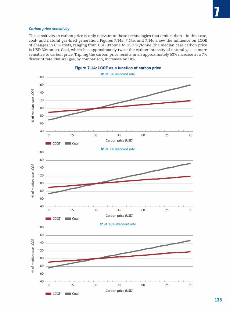
133

7

133

Carbon price sensitivity

The sensitivity to carbon price is only relevant to those technologies that emit carbon – in this case, coal- and natural gas-fired generation. Figures 7.14a, 7.14b, and 7.14c show the influence on LCOE of changes in CO2 costs, ranging from USD 0/tonne to USD 90/tonne (the median case carbon price is USD 30/tonne). Coal, which has approximately twice the carbon intensity of natural gas, is more sensitive to carbon price. Tripling the carbon price results in an approximately 53% increase at a 7% discount rate. Natural gas, by comparison, increases by 18%.

Figure 7.14: LCOE as a function of carbon price

a: at 3% discount rate

% o

f med

ian

case

LCO

E

CoalCCGT

40

60

80

100

120

140

160

180

90 75 60 45 30 15 0

90 75 60 45 30 15 0

90 75 60 45 30 15 0

Carbon price (USD)

% o

f med

ian

case

LCO

E

CoalCCGT

40

60

80

100

120

140

160

180

Carbon price (USD)

% o

f med

ian

case

LCO

E

CoalCCGT

40

60

80

100

120

140

160

180

Carbon price (USD)

b: at 7% discount rate

% o

f med

ian

case

LCO

E

CoalCCGT

40

60

80

100

120

140

160

180

90 75 60 45 30 15 0

90 75 60 45 30 15 0

90 75 60 45 30 15 0

Carbon price (USD)

% o

f med

ian

case

LCO

E

CoalCCGT

40

60

80

100

120

140

160

180

Carbon price (USD)

% o

f med

ian

case

LCO

E

CoalCCGT

40

60

80

100

120

140

160

180

Carbon price (USD)

c: at 10% discount rate

% o

f med

ian

case

LCO

E

CoalCCGT

40

60

80

100

120

140

160

180

90 75 60 45 30 15 0

90 75 60 45 30 15 0

90 75 60 45 30 15 0

Carbon price (USD)

% o

f med

ian

case

LCO

E

CoalCCGT

40

60

80

100

120

140

160

180

Carbon price (USD)

% o

f med

ian

case

LCO

E

CoalCCGT

40

60

80

100

120

140

160

180

Carbon price (USD)

Part 3Boundary issues

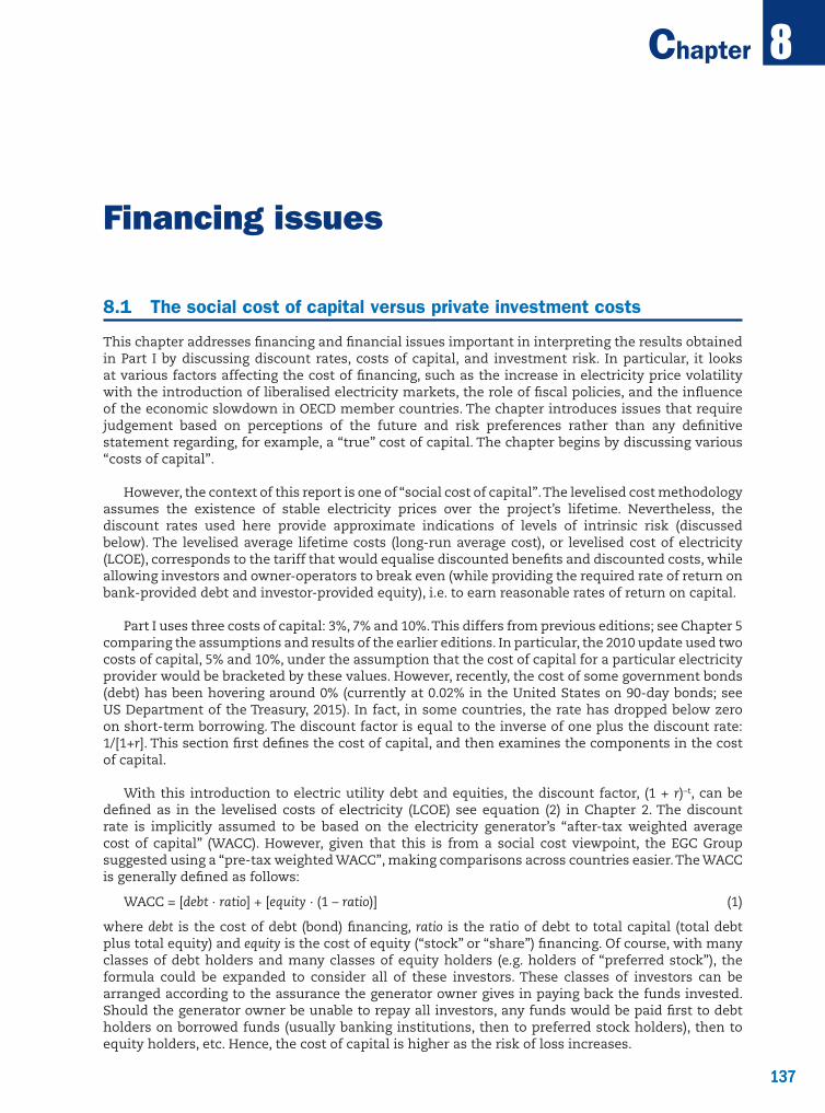
137

8

137

Chapter

Financing issues

8.1 The social cost of capital versus private investment costs

This chapter addresses financing and financial issues important in interpreting the results obtained in Part  I by discussing discount rates, costs of capital, and investment risk. In particular, it looks at various factors affecting the cost of financing, such as the increase in electricity price volatility with the introduction of liberalised electricity markets, the role of fiscal policies, and the influence of the economic slowdown in OECD member countries. The chapter introduces issues that require judgement based on perceptions of the future and risk preferences rather than any definitive statement regarding, for example, a “true” cost of capital. The chapter begins by discussing various “costs of capital”.

However, the context of this report is one of “social cost of capital”. The levelised cost methodology assumes the existence of stable electricity prices over the project’s lifetime. Nevertheless, the discount rates used here provide approximate indications of levels of intrinsic risk (discussed below). The levelised average lifetime costs (long-run average cost), or levelised cost of electricity (LCOE), corresponds to the tariff that would equalise discounted benefits and discounted costs, while allowing investors and owner-operators to break even (while providing the required rate of return on bank-provided debt and investor-provided equity), i.e. to earn reasonable rates of return on capital.

Part I uses three costs of capital: 3%, 7% and 10%. This differs from previous editions; see Chapter 5 comparing the assumptions and results of the earlier editions. In particular, the 2010 update used two costs of capital, 5% and 10%, under the assumption that the cost of capital for a particular electricity provider would be bracketed by these values. However, recently, the cost of some government bonds (debt) has been hovering around 0% (currently at 0.02% in the United States on 90-day bonds; see US Department of the Treasury, 2015). In fact, in some countries, the rate has dropped below zero on short-term borrowing. The discount factor is equal to the inverse of one plus the discount rate: 1/[1+r]. This section first defines the cost of capital, and then examines the components in the cost of capital.

With this introduction to electric utility debt and equities, the discount factor, (1 + r)–t, can be defined as in the levelised costs of electricity (LCOE) see equation (2) in Chapter 2. The discount rate is implicitly assumed to be based on the electricity generator’s “after-tax weighted average cost of capital” (WACC). However, given that this is from a social cost viewpoint, the EGC Group suggested using a “pre-tax weighted WACC”, making comparisons across countries easier. The WACC is generally defined as follows:

WACC = [debt · ratio] + [equity · (1 – ratio)] (1)

where debt is the cost of debt (bond) financing, ratio is the ratio of debt to total capital (total debt plus total equity) and equity is the cost of equity (“stock” or “share”) financing. Of course, with many classes of debt holders and many classes of equity holders (e.g. holders of “preferred stock”), the formula could be expanded to consider all of these investors. These classes of investors can be arranged according to the assurance the generator owner gives in paying back the funds invested. Should the generator owner be unable to repay all investors, any funds would be paid first to debt holders on borrowed funds (usually banking institutions, then to preferred stock holders), then to equity holders, etc. Hence, the cost of capital is higher as the risk of loss increases.

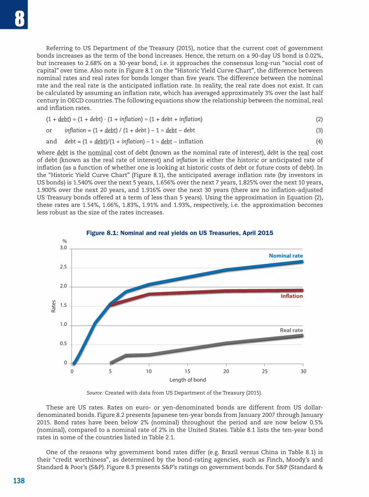
138

8

138

Referring to US Department of the Treasury (2015), notice that the current cost of government bonds increases as the term of the bond increases. Hence, the return on a 90-day US bond is 0.02%, but increases to 2.68% on a 30-year bond, i.e. it approaches the consensus long-run “social cost of capital” over time. Also note in Figure 8.1 on the “Historic Yield Curve Chart”, the difference between nominal rates and real rates for bonds longer than five years. The difference between the nominal rate and the real rate is the anticipated inflation rate. In reality, the real rate does not exist. It can be calculated by assuming an inflation rate, which has averaged approximately 3% over the last half century in OECD countries. The following equations show the relationship between the nominal, real and inflation rates.

(1 + debt) = (1 + debt) · (1 + inflation) ≈ (1 + debt + inflation) (2)

or inflation = (1 + debt) / (1 + debt ) – 1 ≈ debt − debt (3)

and debt = (1 + debt)/(1 + inflation) – 1 ≈ debt − inflation (4)

where debt is the nominal cost of debt (known as the nominal rate of interest), debt is the real cost of debt (known as the real rate of interest) and inflation is either the historic or anticipated rate of inflation (as a function of whether one is looking at historic costs of debt or future costs of debt). In the “Historic Yield Curve Chart” (Figure 8.1), the anticipated average inflation rate (by investors in US bonds) is 1.540% over the next 5 years, 1.656% over the next 7 years, 1.825% over the next 10 years, 1.900% over the next 20 years, and 1.916% over the next 30 years (there are no inflation-adjusted US Treasury bonds offered at a term of less than 5 years). Using the approximation in Equation (2), these rates are 1.54%, 1.66%, 1.83%, 1.91% and 1.93%, respectively, i.e. the approximation becomes less robust as the size of the rates increases.

Figure 8.1: Nominal and real yields on US Treasuries, April 2015

0

0.5

1.0

1.5

2.0

2.5

3.0

0 5 10 15 20 25 30

Rate

s

Length of bond

Real rate

In�ation

Nominal rate

%

Source: Created with data from US Department of the Treasury (2015).

These are US rates. Rates on euro- or yen-denominated bonds are different from US dollar-denominated bonds. Figure 8.2 presents Japanese ten-year bonds from January 2007 through January 2015. Bond rates have been below 2% (nominal) throughout the period and are now below 0.5% (nominal), compared to a nominal rate of 2% in the United States. Table 8.1 lists the ten-year bond rates in some of the countries listed in Table 2.1.

One of the reasons why government bond rates differ (e.g. Brazil versus China in Table 8.1) is their “credit worthiness”, as determined by the bond-rating agencies, such as Finch, Moody’s and Standard & Poor’s (S&P). Figure 8.3 presents S&P’s ratings on government bonds. For S&P (Standard &

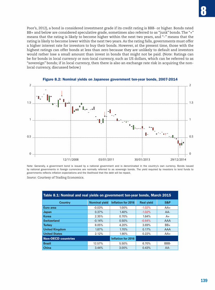
139

8

139

Poor’s, 2012), a bond is considered investment grade if its credit rating is BBB- or higher. Bonds rated BB+ and below are considered speculative grade, sometimes also referred to as “junk” bonds. The “+” means that the rating is likely to become higher within the next two years, and “–” means that the rating is likely to become lower within the next two years. As the rating falls, governments must offer a higher interest rate for investors to buy their bonds. However, at the present time, those with the highest ratings can offer bonds at less than zero because they are unlikely to default and investors would rather lose a small amount than invest in bonds that might not be paid. (Note: Ratings can be for bonds in local currency or non-local currency, such as US dollars, which can be referred to as “sovereign” bonds; if in local currency, then there is also an exchange rate risk in acquiring the non-local currency, discussed below.)

Figure 8.2: Nominal yields on Japanese government ten-year bonds, 2007-2014 2

1.5

1

0.5

0

2

1.5

1

0.5

0

12/11/2008 03/01/2011 30/01/2013 29/12/2014

Note: Generally, a government bond is issued by a national government and is denominated in the country’s own currency. Bonds issued by national governments in foreign currencies are normally referred to as sovereign bonds. The yield required by investors to lend funds to governments reflects inflation expectations and the likelihood that the debt will be repaid.

Source: Courtesy of Trading Economics.

Table 8.1: Nominal and real yields on government ten-year bonds, March 2015

Country Nominal yield Inflation for 2016 Real yield S&P

Euro area -0.03% 1.00% -1.02% AA+Japan 0.37% 1.40% -1.02% AA-Korea 2.35% 0.70% 1.64% A+Switzerland -0.14% 0.50% -0.64% AAATurkey 8.05% 4.20% 3.69% BB+United Kingdom 1.87% 1.70% 0.17% AAAUnited States 2.12% 1.90% 0.22% AA+

Non-OECD countries Inflation for 2016

Brazil 12.57% 5.50% 6.70% BBB-China 3.44% 3.00% 0.43% AA-

140

8

140

Figure 8.3: Standard and Poor’s government bond ratings

AAA AA A BBB BB B CCC

Source: Standard & Poor’s, Sovereigns Ratings List.

Of course, electricity generator owners cannot borrow at the same rate as governments can, because the risk of default on a bond issued by a seller of electricity is higher than the risk of default by a government. In general, the rate on a corporate bond must be at least as high as the rate charged to the government in which the corporate entity has its headquarters. Determining this location can be difficult, except for state-owned electric utilities. For example, EDF is headquartered in France, but has assets in many European countries. Its S&P credit rating is A+, whereas the credit rating of France is AA. The Tennessee Valley Authority is headquartered in the United States. It has historically had credit rating of AAA, but has been lowered to AA+ when the US rating was lowered to AA+.

On the other hand, corporate (shareholder-owned) electric utilities generally have lower ratings on their bonds. According to the Edison Electric Institute (2014):

“The table ‘S&P Utility Credit Rating Distribution by Company Category’ presents the distribution of credit ratings over time for the shareholder-owned electric utilities organized into Regulated, Mostly Regulated and Diversified categories. Ratings are based on S&P long-term issuer ratings at the holding company level, with only one rating assigned per company. At 30 June 2014, the categories had the following average ratings: Regulated = BBB+, Mostly Regulated = BBB+, and Diversified = BBB.”

Further, corporate equities (stocks) are much more difficult to evaluate. One method is to look at how they perform in a portfolio of equities: it is not just the return on the equity that matters, but the correlation between the return and the return in the stock market as a whole. One method for making this calculation is with the Capital Asset Pricing Model, CAPM, and using the firm-specific or project-specific return, and its correlation with a portfolio of assets. The investor expected return on an electric utility, “j” equity, E(equityj), can be evaluated as

E(equityj) = riskfree + betaj ⋅ E(market − riskfree) (5)

where riskfree is the return on, for example, 90-day US Treasury bonds (as discussed above); market is the return on a market portfolio, e.g. Dow Jones index; E(market − riskfree) is the expected difference between the riskfree asset’s return and market portfolio’s rate of return, and betaj is the covariance between equityj and market, divided by the variance of the return on the market. For example, if riskfree were 0% per year and E(market − riskfree) were 8% per year, then the expected return on the market portfolio (where betaj = 1) would be 8%. In fact, the expected average annual market return has been calculated by S&P (2014) for its Dow Jones Index during the last ten years as 8.12%.

In addition, the “beta” of a particular electric utility traded in a major stock market is relatively easy to find if the equity is traded in an established stock market. One source has calculated the long-run beta for US (general) utilities without considering debt leverage as 0.42; (Damodaran, 2015, at the Stern Business School of New York University). Another source, Competition Economist Group, 2013, calculated the long-run beta for US “mostly regulated power utilities” as 0.36 and for US “highly regulated power utilities” at 0.35.

141

8

141

Therefore, with a nominal risk-free rate of 3% on a 30-year bond (see Figure 8.1), an electric utility beta of 0.4, and a nominal market rate of return of 8%, the expected return on an average electricity utility would be about 3% + 0.4 ⋅ (8.12% − 3%) = 5% nominal, or about 3% real on an average (US) electric utility equity. The nominal rate of return on electric utility bonds was about 5% in 2013, or about 3% real (Bank of America/Merrill Lynch, 2013, pp. 57-59). With 50% debt and 50% equity, the WACC has been about 3% real. Something appears to be wrong with this picture and therefore it is important to review project risk, discussed in the next section.

8.2 Private investment costs under uncertainty

Matters change radically when considering investments in competitive electricity markets with uncertain input costs, output prices, and sales. Market risks require higher rates of return on investment, implying higher capital costs. An alternative would be to buy insurance. The cost of insurance, however, would still require that private investors demand a higher rate of return (profit) on their investments than governments. Loan guarantees for new construction are one of these types of insurance. Government guarantees that loans for power plant construction are provided at a price (through a premium) that provides for the default of repayment on the underlying bonds.

Even the most credit-worthy private investors are required to pay a premium over the risk-free rate for their debts, for example the corporate “prime rate”. The longer the period, the higher is the premium. In addition, these investors must make provisions for uncertainty in electricity prices. A sudden drop in prices can turn a promising project into a substantial loss. Because of such uncertainty, risk-averse investors (or their managers) demand average returns higher than the risk-free rate. That means that an investor who will have a zero return on investment if prices are low and a return of 10% if prices are high (assuming there is a fifty/fifty chance of prices being high or low) will not demand an average return of 5% but of, say, 7%. Through the mark-up of 2%, the difference here between the average and the required return, investors seek to compensate themselves for the riskiness of their investments. For electric utilities in rate-of-return regulated environments, a 7% cost of capital is considered an appropriate approximation. For electric utilities competing in liberalised markets, a 10% real cost of capital is considered more appropriate.

This required higher rate of return corresponds to the higher discount rate a private investor will apply when comparing the total discounted costs and benefits of a particular investment. The riskier the investment, the higher will be the mark-up over the average return. Higher costs of capital have a direct influence on the overall cost of projects. To the extent that they reflect the uncertainty faced by private investors, private financial costs are always higher than social costs.

However, the difference between social cost and private financial cost should not be overplayed. Many investors in electricity markets are large, diversified, frequently international companies that operate in many market environments and have substantial abilities of their own to pool returns from a large number of projects and to spread the risks over large numbers of investors. In addition, even if prices have grown more volatile in recent years, underlying demand has been stable (although not growing). Capital markets are aware of this and, generally, electric utilities have easier access to credit and benefit more from some of the lower costs of borrowing in the market than other entities.

In the electricity sector, the difference between social cost and private investment cost (including risk) can vary in response to additional risk factors that are specific to countries, technologies, projects, and prices. Price volatility affects different technologies in various ways. In electricity markets, prices are set by the cost of the marginal fuel, which implies the fuel with the highest variable cost, which is frequently natural gas. For technologies with high fixed cost and low variable cost such as nuclear or renewable, profitability is heavily affected by changing prices for electricity, or, when specific technologies such as solar and wind, have dispatch priority, subsidies, or special feed-in tariffs. This is the most relevant issue in distinguishing the calculations of social cost for baseload power generation under an assumption of stable prices that is adopted here from the cost-benefit calculations of a private investor in liberalised markets.

142

8

142

Many of these risks are in some way related to the regulatory or political sphere. They include the following:

Country-level risks: fiscal policy uncertainties, energy security and exchange rate risk

• regulatory risk (this includes both the regulation of the electricity market, environmental regulations concerning climate change, and other emissions and safety regulations that influence all electricity generators in a particular country);

• changes in fiscal policy, in particular with respect to changes in taxes, which affect capital-intensive technologies, such as nuclear and renewable energy technologies.

Technology risks: capital intensity, first-of-a-kind deployment, and externality internalisation

• technological risks for new technologies such as specific renewable energies (standardisation and design homogenisation can decrease this risk);

• high amounts of capital-at-risk and high ratios of fixed or sunk costs to total cost ratios that limit flexibility when market conditions change;

• safety and human health risks (airborne pollution, radiation leaks, site contamination, major accidents);

• proliferation risk for nuclear fuels and technology;

• availability of long-term options for decommissioning, waste storage and site restoration (especially for nuclear and brown coal);

• risks associated with weather conditions, either poor long-term wind conditions or reduced solar energy due to cloud cover.

Project risks: licensing and regulatory risks

• political risk at the local level (e.g. water access for steam-based power) pertaining to the acceptability of new power generation investments.

Input and output quantities, cost, price and revenue risks and probabilities

• changes in input prices that will affect in particular technologies relying on fossil fuels;

• availability of adequate human resources, skills and knowledge (especially for advanced technologies such as nuclear);

• security of supply risks for the availability of specific inputs, in particular natural gas;

• risks associated with selling into liberalised markets where there are few customers without long-term contracts, where smaller independent generators find it difficult to sell their electricity or green certificates.

This list of the various risks faced by investors in power generation shows that not all technologies are affected by all dimensions of risk in an identical manner, although it is less obvious that one technology does better or worse than the others on all counts. However, despite the important concerns behind the items on this list, their collective influence should not be overestimated.

The exception is price risk for fossil fuels, in particular natural gas. While fuel price risks can to some extent be hedged in many OECD markets, this becomes expensive beyond one or two years. However, the one risk a private investor in power generation in an OECD country is likely to worry about most, and which is also most likely to affect their discount rate and financial cost, remains the revenue risk in competitive electricity markets, particularly in an environment of slow and uncertain demand recovery.

143

8

143

Finally, consider the financial structure of energy investments, which depend directly and immediately on government policy. Investors essentially have two options for raising the funds needed to finance a project: debt and equity. Debt means obtaining credit from a bank. Equity means selling shares in the project to capital markets. Debt is less risky for the lender, owing to higher seniority in case of bankruptcy, is more difficult to access for the borrower, and has stable interest payments. The tax treatment of debt is also frequently more favourable, i.e. interest is considered a cost and is thus tax deductible, while dividends are not. Equity instead is wiped out in case of bankruptcy and its level varies with profits (see the specific discussion below). Necessarily lower-risk debt thus requires lower interest rates than higher-risk equity. The full financial cost of an investment will thus be determined by the interest rates of debt and equity weighted by their respective shares in the financing mix and adjusted for taxes. This average is known as the weighted average cost of capital (WACC). The underlying algorithms of the EGC report calculate financing costs for one single interest rate at a time (either 3% real, i.e. net of inflation, 7% real, or 10% real), without specifying any particular split between debt and equity finance.

Without going into the subtleties of corporate finance a real-world investor must face, one can make the following broad statements in the context of the EGC report. Such a report would need to include, among other issues, accounting conventions, tax laws, the availability of investment incentives, the structure of electricity markets and demand, etc. for one particular market and technology. It could never produce comparable results for many various technologies across many countries according to simple, harmonised assumptions.

8.3 Questionnaire responses regarding the costs of capital and discount rates

The EGC questionnaire included questions regarding the cost of capital for each technology. Table 8.2 presents these data. Some countries provided data for some technologies (certain data were considered confidential and therefore are not presented in the table). The “cost of capital” averages about 7% overall, except for non-conventional technologies in the United Kingdom. The cost of debt ranges between 3.8% and 6% (real), which corresponds to the range for BB+ to BBB- in Table 8.1. The cost of equity ranges from 6% in Germany for residential rooftop solar PV to 15% for renewables in the Netherlands. These rates are generally higher than one would except in the equities markets, reflecting the risks discussed in Section 8.2. Given that the costs of capital are generally between 3% and 10% with an average of 7%, the use of 3%, 7% and 10% in Part I is justified by member country responses.

In summary, a 3% real discount rate would be used by government-owned utilities in countries with good bond ratings or ones with stable rate-of-return regulation and fuel price increase allowances. (Government-owned utilities in countries with poor bond ratings would need to use a higher discount rate.) The 7% real discount rate can be considered as the rate available to an investor with a low risk of default in a stable environment. Traditionally, this was thought of as the risk faced by an electric utility in a regulated market. However, the same rate may apply to a private investor investing in a low-risk technological option in a favourable market environment. The 10% real discount rate instead was considered as the investment cost of an investor facing substantially greater financial, technological and price risks. Any of the qualitative risk factors mentioned above could contribute to this higher rate of discount. Next to price risk, the risk of investing in new and unproven technological options ranks among the most important factors driving up discount rates for investors in the power sector of OECD countries.

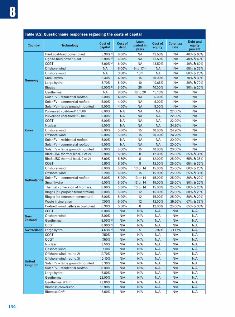
144

8

144

Table 8.2: Questionnaire responses regarding the costs of capital

Country Technology Cost of capital

Cost of debt

Loan period in

years

Cost of equity

Corp. tax rate

Debt and equity

percent

Germany

Hard coal-fired power plant 6.90%(a) 6.00% NA 13.50% NA 40% & 60%Lignite-fired power plant 6.90%(a) 6.00% NA 13.50% NA 40% & 60%CCGT 6.90%(a) 6.00% NA 13.50% NA 40% & 60%Offshore wind NA 6.00% 9 to 17(e) NA NA 65% & 35%Onshore wind NA 3.80% 15(e) NA NA 80% & 20%Small hydro 6.40% 4.50% 15 10.00% NA 70% & 30%Large hydro 6.70% 5.00% 10 10.65% NA 30% & 70%Biogas 6.00%(b) 5.00% 20 10.00% NA 80% & 20%Geothermal NA 6.00% 10 to 20 13.10% NA NASolar PV – residential rooftop 5.00% 4.00% NA 6.00% NA NASolar PV – commercial rooftop 5.00% 4.00% NA 8.00% NA NASolar PV – large ground-mounted 5.00% 4.00% NA 8.00% NA NA

Korea

Pulverised coal-fired/PC 800 6.00% NA NA NA 22.00% NAPulverised coal-fired/PC 1000 6.00% NA NA NA 22.00% NACCGT 6.00% NA NA NA 22.00% NANuclear 6.00% NA NA NA 24.20% NAOnshore wind 6.00% 5.00% 15 10.00% 24.20% NAOffshore wind 6.00% 5.00% 15 10.00% 24.20% NASolar PV – residential rooftop 6.00% NA NA NA 20.00% NASolar PV – commercial rooftop 6.00% NA NA NA 20.00% NASolar PV – large ground-mounted 6.00% 5.00% 15 10.00% 20.00% NA

Netherlands

Black USC thermal (coal, 1 of 2) 6.90% 5.50% 8 12.00% 25.00% 65% & 35%Black USC thermal (coal, 2 of 2) 6.90% 5.50% 8 12.00% 25.00% 65% & 35%CCGT 6.90% 5.50% 8 12.00% 25.00% 65% & 35%Onshore wind 6.00% 5.00% 13 or 14 15.00% 25.00% 80% & 20%Offshore wind 8.20% 6.00% 15 15.00% 25.00% 65% & 35%Solar PV – commercial rooftop 6.00% 5.00% 13 or 14 15.00% 25.00% 80% & 20%Small hydro 6.00% 5.00% 13 or 14 15.00% 25.00% 80% & 20%Thermal conversion of biomass 6.00% 5.00% 13 or 14 15.00% 25.00% 80% & 20%Biogas (all-purpose fermentation) 6.00% 5.00% 12 15.00% 25.00% 80% & 20%Biogas (co-fermentation/manure) 6.00% 5.00% 12 15.00% 25.00% 80% & 20%Waste incineration 7.00% 6.00% 12 12.00% 25.50% 67% & 33%Co-fired wood pellets in coal plant 6.90% 5.50% 8 12.00% 25.00% 65% & 35%

New Zealand

CCGT 8.00% N/A N/A N/A N/A N/AOnshore wind 8.00% N/A N/A N/A N/A N/AGeothermal 8.00%(c) N/A N/A N/A N/A N/AOCGT 8.00%(c) N/A N/A N/A N/A N/A

Switzerland Large hydro 4.63%(a) N/A 5 7.97% 21.17% N/A

United Kingdom

CCGT 7.50% N/A N/A N/A N/A N/AOCGT 7.50% N/A N/A N/A N/A N/ANuclear 9.50% N/A N/A N/A N/A N/AOnshore wind 7.10% N/A N/A N/A N/A N/AOffshore wind (round 2) 9.70% N/A N/A N/A N/A N/AOffshore wind (round 3) 10.10% N/A N/A N/A N/A N/ASolar PV – large ground-mounted 5.30% N/A N/A N/A N/A N/ASolar PV – residential rooftop 8.00% N/A N/A N/A N/A N/ALarge hydro 5.80% N/A N/A N/A N/A N/AGeothermal 22.00% N/A N/A N/A N/A N/AGeothermal (CHP) 23.80% N/A N/A N/A N/A N/ABiomass conversion 10.90% N/A N/A N/A N/A N/ABiomass CHP 13.60% N/A N/A N/A N/A N/A

145

8

145

Table 8.2 (cont’d)

Country Technology Cost of capital

Cost of debt

Loan period in

years

Cost of equity

Corp. tax rate

Debt and equity

percent

United States

Supercritical pulverised coal 5.00%(d) 4.40% N/A 8.30% 39.30% 50% & 50%CCGT 5.00%(d) 4.40% N/A 8.30% 39.30% 50% & 50%Nuclear 5.00%(d) 4.40% N/A 8.30% 39.30% 50% & 50%Onshore wind 5.00%(d) 4.40% N/A 8.30% 39.30% 50% & 50%Offshore wind 5.00%(d) 4.40% N/A 8.30% 39.30% 50% & 50%Solar PV – large ground-mounted 5.00%(d) 4.40% N/A 8.30% 39.30% 50% & 50%Solar CSP 5.00%(d) 4.40% N/A 8.30% 39.30% 50% & 50%Solar CSP 5.00%(d) 4.40% N/A 8.30% 39.30% 50% & 50%Solar CSP 5.00%(d) 4.40% N/A 8.30% 39.30% 50% & 50%Geothermal – flash 5.00%(d) 4.40% N/A 8.30% 39.30% 50% & 50%Geothermal – low temp 5.00%(d) 4.40% N/A 8.30% 39.30% 50% & 50%Solid biomass 5.00%(d) 4.40% N/A 8.30% 39.30% 50% & 50%

Notes: (a) Weighted average cost of capital; (b) nominal; (c) government proscribed; (d) after tax; (e) site-specific.

8.4 Options for improving investment conditions in the power sector

The importance of managing uncertainty makes a strong argument for exploring the possibilities of public-private partnerships to improve the investment conditions in the electricity sector in general, and in particular for capital-intensive, low-carbon technologies such as nuclear and renewables. Few argue for a return to an all public provision of electric power with its inefficiencies and inertia (although 40% of the electric utilities in the United States are still under rate-of-return regulation). The momentum towards liberalised electricity markets in OECD countries has not been reversed, but is in a steady state of reform, for example regarding the compensation of fixed (capacity) costs.

However, even within the broad context of competitive electricity markets, there is a case to be made that the public sector has a role to play in enlarging the choices available to private decision makers. This role must necessarily focus on the reduction of uncertainty to enable investors to benefit from lower costs of capital. There are two fundamental strategies to go about this. First, the overall policy framework for the coming decades must be as stable and as transparent as possible, for example regarding greenhouse gas emissions reduction targets. The remaining uncertainties are enormous, and it would be desirable that future policy actions aim at providing further clarity on the precise implementation of such targets.

The second strategy consists of directly aiming at lowering the cost of capital for investments in the power sector, with or without conditionality on carbon performance. At the national level, OECD countries can, for instance, provide loan guarantees as an incentive measure that would lower the cost of capital – as is being done for low-carbon generators in the United Kingdom. (Of course, government loan guarantees charge fees similar to those that would be charged in financial markets; hence, this is one way to overcome capital market failures in providing new electric capacity in a risky liberalised electricity market.) In addition, such a measure would be compatible with the workings of competitive power markets. Some OECD countries are currently moving in this direction.

At the international level, multilateral institutions such as the World Bank or the development banks for Africa, Asia and Latin America can also facilitate investment by reducing risk through loan guarantees. Export credit guarantees already play a role in this context. While these international development banks could play useful roles in reducing investment risk, they cannot be drawn upon as an exclusive source of finance, since they do not treat all technologies alike. The African Development Bank, the Asian Development Bank and the Inter-American Development Bank have policies in place not to finance nuclear energy projects. The European Bank for Reconstruction and Development provides nuclear safety grants, but does not finance new nuclear reactors. Finally, the World Bank has no written policy on nuclear energy, but has not financed nuclear projects for nearly a half-century.

146

8

146

The case for improving the financing context and lowering the cost of capital whenever possible is warranted also from a sustainable development perspective. If sustainable investment is, in the words of the Brundtland definition about “development that meets the needs of the present without compromising the ability of future generations to meet their own needs”, then the future should not be discounted too steeply. Ensuring a stable investment environment with low real interest rates is one of the most effective steps to ensure sustainable development in the electricity sector and beyond, given the deflationary era into which some OECD countries could be slipping.

References

Bank of America/Merrill Lynch (2012), “Electrics & Power: 2013 Outlook/2012 Review”, http://ipu.msu.edu/surfa/presentations/2013/BofAML%20Electrics%20&%20Power%202013%20Outlook%2008%20Jan%202013.pdf.

Competition Economist Group (2013), “Information on equity beta from US companies”, www.aer.gov.au/sites/default/files/Report%209%20-%20US%20Beta%20Comparables%20(Final)%20-%2027%20June.pdf.

Damodaran, A. (2015), “Betas by Sector (US)”, http://people.stern.nyu.edu/adamodar/New_Home_Page/datafile/Betas.html.

Edison Electric Institute (2014), “Q2 2014 Credit Ratings”, www.eei.org/resourcesandmedia/industrydataanalysis/industryfinancialanalysis/QtrlyFinancialUpdates/Documents/QFU_Credit/ 2014_Q2_Credit_Ratings.pdf.

Standard & Poor’s (2012), “Standard & Poor’s Ratings Definitions”, Standard & Poor’s Global Credit Portal, www.standardandpoors.com/spf/general/RatingsDirect_Commentary_979212_06_22_ 2012_12_42_54.pdf.

Standard & Poor’s (2014), “Dow Jones Industrial Average”, Dow Jones Indices-McGraw Hill Financial, www.djindexes.com/mdsidx/downloads/fact_info/Dow_Jones_Industrial_Average_Fact_Sheet.pdf.

US Department of the Treasury (2015), “Historic Yield Curve Chart”, Resource Center, updated 2 March 2015, www.treasury.gov/resource-center/data-chart-center/interest-rates/Pages/TextView.aspx?data=yield.

147

9

147

Chapter

Emerging generating technologies

This chapter aims to provide a summary of emerging technologies in the power generation sector which are currently at demonstration and early deployment stage. The technologies have been selected on the basis of their potential to reach commercialisation in the 2025 to 2030 time frame, as well as for prospects to support electricity security and power-sector decarbonisation goals.

A total of 11 emerging technologies have been identified that could begin to play a larger role in the electricity sector over the next decade and a half. A summary has been provided for each technology and includes a brief technology description, current status and future potential; a description of the role of the technology within the generation market and the advantages offered compared to current technologies; where possible current cost and performance data as well as prospects for future improvements; and barriers to further development and deployment as well as recommendations on how to overcome these barriers.

The emerging technologies covered in this chapter are:

• high-efficiency low-emission coal: integrated gasification combined-cycle (IGCC) and advanced ultra-supercritical (A-USC);

• carbon capture and storage (CCS);

• fuel cells;

• enhanced geothermal systems;

• emerging solar photovoltaics (PV);

• emerging solar thermal electricity;

• floating and deep offshore wind;

• emerging bioenergy technologies;

• ocean energy technologies;

• electricity storage technologies;

• emerging nuclear technologies (small modular reactors and generation IV reactors – gen IV).

Governments have a major role to play in supporting innovative research and development, in developing policies to support market creation, and in co-operating with industry and the financial sector to develop appropriate market conditions so as to allow technologies to overcome barriers. Careful planning is required to ensure that limited resources are devoted to the highest-priority, highest-impact actions in the near term, while laying the groundwork for longer-term improvements.1

1. Much uncertainty remains about the learning effects considered in the following sections for the 2030 horizon and the results which are presented. Depending on the development status, the ranges of possible LCOE for the different technologies remain still very large at that horizon and the results must be taken very carefully. The ranges considered here are mainly derived from IEA analyses or literature reviews and have not been vetted by the EGC Expert Group.

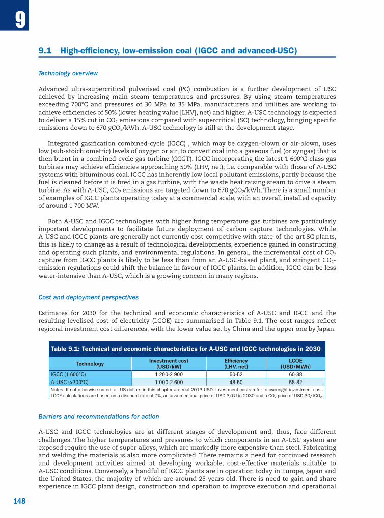
148

9

148

9.1 High-efficiency, low-emission coal (IGCC and advanced-USC)

Technology overview

Advanced ultra-supercritical pulverised coal (PC) combustion is a further development of USC achieved by increasing main steam temperatures and pressures. By using steam temperatures exceeding 700°C and pressures of 30  MPa to 35  MPa, manufacturers and utilities are working to achieve efficiencies of 50% (lower heating value [LHV], net) and higher. A-USC technology is expected to deliver a 15% cut in CO2 emissions compared with supercritical (SC) technology, bringing specific emissions down to 670 gCO2/kWh. A-USC technology is still at the development stage.

Integrated gasification combined-cycle (IGCC) , which may be oxygen-blown or air-blown, uses low (sub-stoichiometric) levels of oxygen or air, to convert coal into a gaseous fuel (or syngas) that is then burnt in a combined-cycle gas turbine (CCGT). IGCC incorporating the latest 1 600°C-class gas turbines may achieve efficiencies approaching 50% (LHV, net); i.e. comparable with those of A-USC systems with bituminous coal. IGCC has inherently low local pollutant emissions, partly because the fuel is cleaned before it is fired in a gas turbine, with the waste heat raising steam to drive a steam turbine. As with A-USC, CO2 emissions are targeted down to 670 gCO2/kWh. There is a small number of examples of IGCC plants operating today at a commercial scale, with an overall installed capacity of around 1 700 MW.

Both A-USC and IGCC technologies with higher firing temperature gas turbines are particularly important developments to facilitate future deployment of carbon capture technologies. While A-USC and IGCC plants are generally not currently cost-competitive with state-of-the-art SC plants, this is likely to change as a result of technological developments, experience gained in constructing and operating such plants, and environmental regulations. In general, the incremental cost of CO2 capture from IGCC plants is likely to be less than from an A-USC-based plant, and stringent CO2-emission regulations could shift the balance in favour of IGCC plants. In addition, IGCC can be less water-intensive than A-USC, which is a growing concern in many regions.

Cost and deployment perspectives

Estimates for 2030 for the technical and economic characteristics of A-USC and IGCC and the resulting levelised cost of electricity (LCOE) are summarised in Table 9.1. The cost ranges reflect regional investment cost differences, with the lower value set by China and the upper one by Japan.

Table 9.1: Technical and economic characteristics for A-USC and IGCC technologies in 2030

Technology Investment cost (USD/kW)

Efficiency (LHV, net)

LCOE (USD/MWh)

IGCC (1 600°C) 1 200-2 900 50-52 60-88A-USC (>700°C) 1 000-2 600 48-50 58-82Notes: If not otherwise noted, all US dollars in this chapter are real 2013 USD. Investment costs refer to overnight investment cost. LCOE calculations are based on a discount rate of 7%, an assumed coal price of USD 3/GJ in 2030 and a CO2 price of USD 30/tCO2.

Barriers and recommendations for action

A-USC and IGCC technologies are at different stages of development and, thus, face different challenges. The higher temperatures and pressures to which components in an A-USC system are exposed require the use of super-alloys, which are markedly more expensive than steel. Fabricating and welding the materials is also more complicated. There remains a need for continued research and development activities aimed at developing workable, cost-effective materials suitable to A-USC conditions. Conversely, a handful of IGCC plants are in operation today in Europe, Japan and the United States, the majority of which are around 25 years old. There is need to gain and share experience in IGCC plant design, construction and operation to improve execution and operational

149

9

149

reliability. Most IGCC plant designs require a substantial amount of oxygen for use in the gasifier; thus IGCC efficiency can be improved by reducing the energy requirements for oxygen production. In addition, research, development and demonstration (RD&D) aimed at adapting higher-efficiency gas turbines – e.g. 1 600°C class – into IGCC plants will improve their overall efficiency. Other important RD&D objectives for IGCC include improving plant reliability and cost reductions; more operational IGCC plants would help in achieving these objectives. The use of lower-grade coals tends to reduce efficiency and raise capital costs for both technologies, though IGCC is generally more tolerant to lower-grade fuels than PC plants. RD&D to mitigate this penalty for USC plants currently focuses on using drying systems for lignite and solid feed pumps. RD&D support is needed to enable timely deployment for both A-USC and IGCC technologies.

9.2 Carbon capture and storage

Technology overview

Carbon capture and storage is a critical technology to allow the continued use of coal, gas and other fossil fuels while achieving ambitious greenhouse gas targets. The use of CCS with biomass can also deliver net removals of CO2 from the atmosphere. The individual component technologies required for CO2 capture, transport and storage are generally well understood and, in some cases, technologically mature. The largest challenge for CCS deployment is the integration of the component technologies into successful large-scale projects. One coal-fired power plant equipped with CCS is in operation, and about ten others are at advanced stages of planning.

Cost and deployment perspectives

The LCOE from coal-fired generation is expected to increase by 30% to 70% by the addition of CO2 capture with currently available capture technologies. By 2030, this cost mark-up could decline through learning effects to a range of 25% to 40%, assuming a deployment level of around 100 GW for coal-fired CCS plants in the IEA’s 2-degree scenario (2DS) (IEA, 2014). Thus, the LCOE from a new USC plant with post-combustion capture is expected to be around USD 90/MWh for plants built in the 2030s in the United States (Table 9.2). For natural gas combined-cycle (NGCC) plants with CO2 capture, the LCOE is very sensitive to the gas price, and could range from around USD 65/MWh in the United States to USD 100/MWh in Asia for plants built in the 2030s. The CO2 price at which these plants with CCS would have the same LCOE as a similar plant without CCS can be expressed by the cost of CO2 avoided, estimates for which could be from around USD 40 to USD 70/tCO2 for coal plants in 2030 (excluding any costs for CO2 transport and storage, which further increases the CO2 price necessary to make the entire CCS chain, not only generation, cost-competitive compared to a plant without CCS); for natural gas combined-cycle plants, this cost ranges from USD 80/tCO2 in the United States to USD 90/tCO2 in Asia.

Table 9.2: Technical and economic characteristics for CCS technologies in 2030

Technology Investment cost (USD/kW)

Efficiency (LHV, net, %)

LCOE (USD/MWh)

Capacity in 2DS (GW)

CO2 captured in 2DS (Mt CO2)

USC post-combustion capture 1 400-3 650 41 50-86102 610USC oxy-fuel combustion 1 500-3 900 41 51-89

IGCC pre-combustion capture 1 500-3 700 44 53-89NGCC post-combustion capture 1 100-1 800 56 65-98 41 100Notes: LCOE calculations are based on a discount rate of 7%, an assumed coal price of USD 3/GJ in 2030 and a gas price range from USD 5.6/GJ in the United States to USD 12/GJ in Asia in 2030. Lower investment costs refer to China, upper costs to the United States. A CO2 price of USD 30/tCO2 has been assumed.

150

9

150

Barriers and recommendations for action

While prospects for incremental (and radical) improvements in capture technologies exist in the longer term, the most significant impediment to the development of capture technologies today is the relatively few opportunities to apply existing technologies at scale (i.e. hundreds of MW). The relative paucity of projects means that technology improvements (and cost reductions) that could emerge from learning-by-doing remain largely unrealised. In the absence of a policy framework that creates near-term opportunities for projects and is expected to drive CCS adoption in the medium term (whether by pricing or regulation), there is little incentive for industry to continue investing in capture technology.

Mobilising the financial resources necessary to build confidence in CCS for power generation and drive down costs depends, in large part, on forward-looking government policy. Urgent action is required from government to develop and implement incentive frameworks that can continue to support CCS demonstration and to promote cost-effective CCS deployment. At the same time, industry must recognise the strategic importance of CCS for their business, and work alongside government to make CCS a reality.

While much of the focus for CCS technology development is on capture, there is also a critical need to support the exploration for and development of storage resources and CO2 transport infrastructure. This could include policies that unlock the synergies between CO2 capture and CO2-enhanced oil recovery (EOR) for long-term storage, where CO2-EOR is an option. Generally, the conditions for transport and storage can vary much according to the country’s local conditions and can have a significant influence on the total cost of that technology.

9.3 Fuel cells

Technology overview

Fuel cells (FCs) are electrochemical devices that generate electricity and heat using hydrogen (H2) or H2-rich fuels, together with oxygen from the air. Compared to other single-stage processes to convert chemical energy into electricity, e.g. open-cycle gas turbines, the efficiency is slightly higher and in the range of 30% to 50%. If pure hydrogen is used, the exhaust of FCs is water vapour.

Between 2008 and 2013 the global market of fuel cells grew by almost 600% (US-DOE, 2014), resulting in more than 150 MW of new nominal FC power capacity by 2012 and a cumulative installed power of around 500 MW (Decourt et al., 2014). While the United States ranks first in terms of added FC power capacity, Japan ranks first in terms of delivered systems, thanks to the successful upscaling of the Enefarm micro-FC combined heat and power large-scale demonstration project.

Different fuel cell types exist, which can mainly be distinguished by their electrolyte type and operating temperature. Molten carbonate FC (MCFC) and solid oxide FC (SOFC) are the main technologies for all stationary applications, while polymer electrolyte membrane FC (PEMFC) are used for small-scale residential applications. MCFC and SOFC operate at higher temperatures of 600-700°C and 600-1 000°C, respectively, which makes them more suitable to combined heat and power applications. FCs are currently used in niche markets for backup, highly reliable or remote power generation.

A trade-off between efficiency and power output exists with fuel cells. Efficiency is highest at very low loads and decreases with power output. Also, the higher the temperature, the better is the efficiency at otherwise similar parameters. There is a need to increase efficiencies at higher loads. On the other side, higher operation temperature results in lower operational flexibility. SOFCs can

151

9

151

achieve very high electric efficiencies at the cost of reduced ability to adapt to changes in electricity demand. Increasing fuel cell efficiencies and utilisation of waste heat are key focus areas for technology development.

Cost and performance perspectives

FCs for stationary power applications are at an early commercialisation phase, with specific investment costs for gas-fired FCs still being four to six times higher compared to combined-cycle plants. With further research and development and increasing deployment, learning effects and large-scale manufacturing could lead to further cost reductions in the future (Table 9.3). For SOFCs, for example, the National Energy Technology Laboratory (NETL) estimates that SOFCs could by 2030 reach investment costs comparable to combined-cycle plants today (NETL, 2013).

Table 9.3: Technical and economic characteristics for FC technologies in 2030

Technology Investment cost (USD/kW) Efficiency Stack lifetimes

(hours)LCOE

(USD/MWh)SOFC 1 100-1 800 55-60

40 000-60 00065-127 (39-100)

MCFC 1 600-3 500 50-55 81-168 (52-140)Notes: LCOE calculations are based on a discount rate of 7% and a gas price range from USD 5.6/GJ in the United States to USD 12/GJ in Asia in 2030. A CO2 price of USD 30/tCO2 has been assumed. Lower LCOE numbers in parentheses take into account an assumed heat credit of USD 45/MWh.

Barriers and recommendations for action

Currently high investment cost and low lifetimes are the biggest barriers for a wider application of fuel cells. Investment costs greatly depend on manufacturing cost, and could be significantly reduced with economies of scale. The reduction of noble metals used as a catalyst is also a priority to reduce cost.

9.4 Enhanced geothermal systems

Technology overview

Enhanced geothermal systems (EGS), also known as hot rock technology, use heat of the Earth where no or insufficient steam or hot water exists and where permeability is low. EGS technology is centred on engineering and creating large heat exchange areas in hot rock. The process involves enhancing permeability by opening pre-existing fractures and/or creating new fractures. Heat is extracted by pumping a transfer medium, typically water, down a borehole into the hot fractured rock and then pumping the heated fluid up another borehole to a power plant, from where it is pumped back down (recirculated) to repeat the cycle.

EGS can be developed in already existing sites with insufficient permeability to develop new plants in locations without geothermal fluid. Since 2008, there is a 1.5 MW demonstration project operating in France, the world’s first grid-connected EGS plant. Other countries outside Europe, notably Australia, China and the United States, are also active in EGS RD&D and evaluating potential pilot sites. In 2013, Geodynamics’ Haberno geothermal project (1  MW) generated electricity from an EGS development, the first in Australia. EGS technologies would allow wider deployment of geothermal technologies, but are currently at the demonstration stage and require further RD&D and experience to become commercially viable.

152

9

152

Cost and deployment perspectives

EGS costs cannot yet be assessed accurately because the limited experience available has only derived from pilot plants where economics are relatively unimportant and whose production cost estimates vary significantly depending on local conditions (depth, resource quality). Therefore, a large degree of uncertainty exists about the future cost reduction potential, reflected in the cost range shown in Table 9.4 for 2030.

Table 9.4: LCOE for EGS technologies in 2030

Technology Investment cost (USD/kW)

Fixed O&M costs

(USD/kW)

LCOE (USD/MWh)

Capacity (GW)

Electricity generation (TWh)

EGS 6 600-20 000 130-390 92-2702 (2DS) 14 (2DS)

8 (2DS hi-Ren) 56 (2DS hi-Ren)Notes: LCOE calculations are based on a discount rate of 7%. Global capacity and electricity generation numbers for EGS in 2030 refer to the 2-degree scenario (2DS) and its high-renewable variant (2DS hi-Ren) of IEA’s Energy Technology Perspectives 2014 (ETP 2014) publication (IEA, 2014).

Barriers and recommendations for action

The main barrier to exploiting geothermal energy is the high cost of drilling. New and innovative techniques for exploration, stimulation and exploitation are needed to make EGS technology commercially viable. Stimulation procedures need to be refined to significantly enhance hydraulic productivity, while reducing the risk associated with induced seismicity. In addition to gaining more experience from new pilot and demonstration plants, efforts should also be expanded to apply EGS techniques to hydrothermal fields. One such concept is to extend existing hydrothermal fields by drilling wells on their boundaries, in appropriate directions with reference to the local stress field, and stimulate them to connect the field to the main hydrothermal reservoir.

Developing EGS requires keeping health, safety and environmental risks as low as reasonably practicable. To mitigate risks related to induced seismicity, strategies are needed to set requirements for seismic monitoring and for prolonged field operation.

9.5 Floating and deep offshore wind

Technology overview

Deep offshore (depths more than 30 m) and floating offshore wind turbines offer attractive opportunities to capture some of the best wind resources. New types of fixed bottom foundations developed with improved knowledge of the sub-surface environment, including tripods, jackets, gravity-based and suction caissons, are currently being tested. For depths exceeding 50 m to 60 m, floating offshore foundations offer the potential to reduce foundation material, simplify installation and decommissioning. New tools will be required to capture the design criteria, which include the need to address weight and buoyancy requirements as well as the heaving and pitching moments created by wave action. Current floating concepts include the spar buoy, tension leg platform and the buoyancy-stabilised, semi-submersible platform.

Offshore turbines could adopt a design other than the mainstream three-blade concept, e.g. two blades rotating downwind of the tower or vertical axis turbines. Improved alternating-current (AC) power take-off systems or the introduction of meshed direct-current (DC) power systems are also promising technologies for internal wind power plant grid offshore and connection to shore. Changes in design architecture and an ability to withstand a wider array of design considerations, including hurricanes, surface icing, and rolling and pitching moments, are also likely to be needed.

153

9

153

Cost and deployment perspectives

Cost reductions of about 40% could be expected in the cost of electricity generation by offshore wind by 2030, though uncertainties remain (Table 9.5). The UK Crown Estate expects cost reductions from areas such as greater competition in key supply markets (e.g. turbines, foundations and installation) and installation with the largest savings from turbine changes (Crown Estate, 2012). Other areas of potential cost reduction include front-end activity, economies of scale, standardisation, improved installation methods and a lower cost of capital.

Table 9.5: LCOE for floating and deep offshore wind technologies in 2015 and 2030

Technology LCOE 2015 (USD/MWh)

LCOE 2030 (USD/MWh)

Capacity 2030 (GW)*

Deep offshore 172-242 104-151 190 (2DS)Floating offshore 187-316 114-189 242 (2DS hi-Ren)* For all offshore wind.

Barriers and recommendations for action

Limited experience with deep offshore plants and the need to demonstrate new types of foundations and floating turbine designs are currently a major barrier to wider deployment of emerging offshore wind technologies. Support for deployment of new designs will help to increase experience and learning which should lead to lower costs. Reliability and other operational improvements would be accelerated through greater sharing of operating experience among industry actors, including experiences related to other marine technologies. Co-ordinating preventive maintenance efforts with improved wind and weather forecasting should allow operators to minimise turbine production losses. Maritime spatial planning that includes areas for offshore wind energy deployment and appropriate offshore planning regimes need to be developed.

9.6 Emerging solar photovoltaics

Technology overview

Although crystalline silicon (c-Si) modules have seen significant improvements in performance, with efficiency of the best commercial c-Si modules now exceeding 21%, target efficiencies of 28% could be reached through the development of tandem (hetero or multi-junction) cells by 2025. The rapid cost decline of c-Si opens the door for mass production of high-efficiency tandem cells, where a thin film would be deposited on c-Si wafers. Such combination would work under “1-sun” (i.e. non-concentrating) PV systems or low concentration with on-axis tracking devices.

Concentrating photovoltaic (CPV) technologies are making progress, but face difficult competition from “1-sun” PV. However, introducing CPV material on the path of light in solar-thermal electricity plants would allow increasing significantly their overall efficiency thanks to a more complete utilisation of the solar spectrum (see solar thermal electricity in Section 9.7).

Cost and deployment perspectives

While rapid deployment has driven most cost reductions over the past decade, technology improvements are likely to return as a major factor behind future reductions, together with the move towards sunnier skies, and with the increasing market maturity reducing financing costs. Extrapolating observed learning curves for PV into the future, LCOE of new utility-scale systems

154

9

154

could fall on average below USD 100/MWh before 2025, while reaching this level before 2025 in the sunniest places. Small rooftop systems could fall on average to USD 95 to 110/MWh by 2030 and gradually reach USD 75/MWh, as a global average with larger ranges owed to the local conditions (Table 9.6).

Table 9.6: LCOE for solar PV in 2015 and 2030

Scenario Technology LCOE 2015 (USD/MWh)

LCOE 2030 (USD/MWh)

Capacity 2030 (GW)

2DSUtility-scale systems 110-294

(164 global average)68-173

(83 global average)841

Rooftop systems 125-499 (186 global average)

77-389(110 global average)

2DS hi-RenUtility-scale systems 110-294

(164 global average)52-129

(75 global average)1 920

Rooftop systems 125-499 (186 global average)

59-214 (94 global average)

Notes: LCOE calculations are based on a discount rate of 7%. Ranges reflect regional differences in costs and solar conditions.

Barriers and recommendations for action

The main areas for policy intervention to support further PV technology development include: removing or alleviating non-economic barriers such as costly and lengthy permitting and connecting procedures; facilitating integration of larger shares of PV in the system; providing innovative financing schemes to reduce costs of capital and supporting RD&D in emerging PV technologies to help develop and demonstrate new modules. Certification of developers, designers and installers, regularly updated, may also improve customer confidence. Finally, grid codes and other regulation could facilitate smoother integration of PV systems into grids.

9.7 Emerging solar thermal electricity (concentrating solar power)

Technology overview

Emerging solar thermal electricity (STE) technologies focus on thermal storage and solar towers which offer a more efficient design than linear systems. Molten-salt towers are particularly attractive as the high temperature difference allows dividing by three the cost of storage – about 12% of the overall investment cost of parabolic trough plants with 7-hour storage.

Solar towers offer the advantage of being less sensitive to seasonal variations than linear systems, which have greater optical losses in winter. Towers also offer a great diversity of designs and present various trade-offs, including the size and number of heliostats that reflect the sunlight onto the receivers atop the tower. There are two basic receiver designs: external and cavity. The cavity design is thought to be more efficient, reducing heat losses, but accepts a limited angle of incoming light. Another important design choice relates to the number of towers for one turbine. To limit optical absorption but benefit from higher efficiency and economies of scale of large turbines, several towers can be linked to one turbine. The possibilities of even higher temperatures should be explored using different receiver technologies which could allow the introduction of supercritical steam turbines in CSP plants.

The next step for STE technology could consist in a full merge with CPV technologies. The combination of both technology families in a single device would allow utilising more fully the solar spectrum and offer a significantly improved combined efficiency, with still about half of the electricity coming from a thermal phase making storage effective and affordable.

155

9

155

Cost and performance perspectives

As deployment of CSP plants increases in areas of higher direct normal irradiance (DNI) such as the south-western United States, North Africa, South Africa, Chile, Australia and the Middle East, better solar resources will be used and improve performance. Increased performance and economies of scale could also reduce LCOE costs of CSP plants. In the 2DS hi-Ren scenario, average LCOE costs of CSP plants with storage could drop below USD 100/MWh around 2030 (Table 9.7).

Table 9.7: LCOE for CSP with storage in 2015 and 2030

Scenario LCOE 2015 (USD/MWh)

LCOE 2030 (USD/MWh)

Capacity 2030 (GW)

2DS 131-190 (152 global average)

87-112 (100 global average) 155

2DS hi-Ren 131-190 (152 global average)

76-100 (86 global average) 252

Notes: LCOE calculations are based on a discount rate of 7%. Ranges reflect regional differences in costs and solar conditions.

Barriers and recommendations for action

Developers have encountered several barriers to establishing CSP plants. These include insufficiently accurate DNI data, inaccurate environmental data; policy uncertainty; difficulties in securing land, water and connections; permitting issues and expensive financing. Policy intervention is needed to remove or alleviate non-economic barriers such as costly and lengthy permitting and connection procedures; tailored incentive schemes to support deployment; innovative financing schemes to reduce costs of capital and strengthened RD&D efforts to further reduce costs.

9.8 Emerging bioenergy technologies

Technology overview

Biomass power plants, using a combustion boiler in combination with a steam turbine to produce electricity (or, in a co-generation design, also heat) represent a generally mature technology. Alternative biomass conversion technologies to the combustion steam cycle exist, with overall higher conversion efficiencies, but have often not yet reached full commercially mature development status. Some of these alternative options are briefly presented here.

The co-firing of biomass with coal in existing large power station boilers has proved to be one of the most cost-effective large-scale means of converting biomass to electricity. Direct co-firing into the boiler is an established and commonly used technology, but the co-firing share without pre-treatment is limited to 5% to 10%. Higher biomass shares can be achieved through indirect co-firing by gasifying the biomass first, but also lead to higher capital costs. Higher costs are also linked with parallel co-firing, which uses a separate biomass boiler for steam generation.

Gasification is a highly versatile process, because virtually any (dry) biomass can be efficiently converted to fuel gas. The produced gas can be used to generate electricity directly via engines or by using gas turbines at higher efficiency than via a steam cycle, particularly in small-scale plants. Gasification-based systems coupled with combined gas and steam turbines provide efficiency advantages compared to combustion but reliability and efficiency of these plants still need to be demonstrated at large scale. Biomass internal combustion gas turbine (BICGT) and biomass internal gasification combined-cycle (BIGCC) are two promising technologies, while gasification with fuel cells are at the RD&D stage.

156

9

156

Cost and performance perspectives

Advanced biomass generation technologies, such as gasification, offer the potential of better generation efficiency and of future cost reductions, but as the systems are so far not deployed on a commercial scale, it is difficult to find reliable cost and operating data. Hence, the ranges below for BIGCC as well as indirect co-firing should be regarded as indicative. For comparison, cost data for conventional steam turbines at a range of scales of operation have been included (Table 9.8).

Table 9.8: LCOE for bioenergy technologies in 2015 and 2030

TechnologyInvestment cost (USD/kW) Efficiency (%) LCOE (USD/MWh)

2015 2030 2015 2030 2015 2030

Direct co-firing 700-1 000 700-1 000 37 40 72-117 67-109Indirect co-firing 3 300-4 400 2 900-3 900 37 40 127-189 115-171Parallel co-firing 1 800-2 800 1 600-2 500 37 40 93-151 85-138Steam cycle (10-50 MW) 4 000-6 000 3 400-4 700 18-30 23-32 78-244 66-192Steam cycle (>50 MW) 3 000-4 300 2 700-3 700 30-35 33-38 118-204 105-181BIGCC 4 800-7 500 4 000-6 200 35-38 42-44 131-219 108-178Notes: LCOE calculations are based on a discount rate of 7%. Feedstock prices are USD 6 to 10/GJ for all technologies, except for the smaller steam-cycle plant with a feedstock cost range of USD 0 to 6/GJ, reflecting the possibility to use process residues.

Barriers and recommendations for action

Biomass electricity can already be competitive with fossil fuels under favourable circumstances today. Through standardising optimised plant designs and improving efficiencies, biomass electricity generation could become competitive with fossil fuels under a CO2 price regime. Enhanced RD&D efforts will bring new technologies to the market. The availability of affordable biomass for electricity generation will require well developed supply chains to mobilise sufficient amounts of biomass with minimal transport of greenhouse gas (GHG) emissions. Poor transport infrastructure can become a critical barrier, in particular in undeveloped rural areas, and should be tackled as part of a rural development strategy. The introduction of internationally aligned technical standards for biomass and biomass intermediates, in order to reduce and eventually abolish trade barriers, can enhance sustainable biomass trade and tap new feedstock sources.

9.9 Ocean energy technologies

Technology overview

Ocean energy covers wave, tidal range, tidal current, ocean thermal energy conversion and salinity gradients. Total global ocean energy capacity is currently 533 MW, with tidal range accounting for most of it. Wave energy and tidal current are the two most active areas with RD&D aiming to overcome technical barriers. The focus is on moorings; structure and hull design methods; power take-off systems; deployment methods and wave behaviour; and the hydrodynamics of wave absorption. Research on tidal current systems can be divided into basic research on areas such as water stream flow patterns and cavitations, and applied science, which examines supporting structure design, turbines, foundations and deployment methods. In-current technologies have the potential to increase tidal range potential, now limited to only sites with very high-level ranges.

Research efforts on turbines and rotors will need to focus on cost-efficiency, reliability and ease of maintenance, particularly in developing components that can resist hostile marine environments. Control systems for turbine speed and rotor pitch will also be important to maximise power output.

157

9

157

The main challenge for salinity gradient systems is to develop functioning and efficient membranes that can generate sufficient energy to make an energy system competitive.

Cost and deployment perspectives

Civil works typically represent more than half the total investment cost for shoreline and near-shoreline installations. The cost structure is different for deep-water devices. As most ocean energy technologies are still at the RD&D stage, current cost data are not very informative. Under optimistic assumptions, assuming more experience from pilot projects is gained, increasing reliability and standard designs for components are reached, stimulating the development of a supply chain, learning effects after 2020 based on a learning rate of 10%, could reach to cost reductions down to USD 125 to 145/MWh by 2030 (Table 9.9). However, given the current development status of ocean technologies, uncertainties still remain about this development pathway, particularly associated with the location under consideration, making it difficult to take advantage of learning effects.

Table 9.9: LCOE for ocean technologies in 2020 and 2030

TechnologyInvestment cost (USD/kW) LCOE (USD/MWh) Capacity

(GW)

2020 2030 2020 2030 2030

Tidal stream 5 100-6 600 3 100-4 000 206-368 124-22115

Wave energy 6 700-10 000 3 700-5 600 260-639 143-351Note: LCOE calculations are based on a discount rate of 7%.

Barriers and recommendations for action

A factor common to all marine technologies is that pilot projects need to be relatively large-scale if they are to withstand offshore conditions. Such projects are costly and carry high commercial risks; hence adequate government funding will be needed to support sizeable pilot projects. Non-technical barriers include the need for resource assessment and energy-production forecasting and design tools, as well as test and measurement standards. Environmental effects pose other challenges. Potential solutions include arrays of farms of ocean energy systems and multi-purpose plants that combine energy generation, energy storage and others (fish-farming, recreation, etc.).

9.10 Electricity storage technologies

Technology overview

Energy storage technologies absorb energy and store it for a period of time before releasing it to supply energy or power services. Through this process, storage technologies can bridge temporal and geographical gaps between energy supply and demand. Some technologies such as pumped storage hydropower are mature; however, improvements can be made with respect to the ratio of electric capacity to storage volume; flexibility in pumping mode with variable-speed pumps; and sea water pumped storage hydropower, to better help integrate variable renewables. Most other technologies are still at the early stages of development and will require further RD&D before their potential can be fully realised. Emerging electricity storage technologies include compressed air energy storage (CAES), adiabatic CAES, a range of batteries, flywheels and hydrogen storage.

Large-scale energy storage capacity is estimated to be over 145 GW in 2013/14 of which over 97% was accounted for by pumped hydro storage. There is also an estimated 2.4 GW of grid-connected thermal energy storage, whose actual value is likely to be significantly higher as applications not

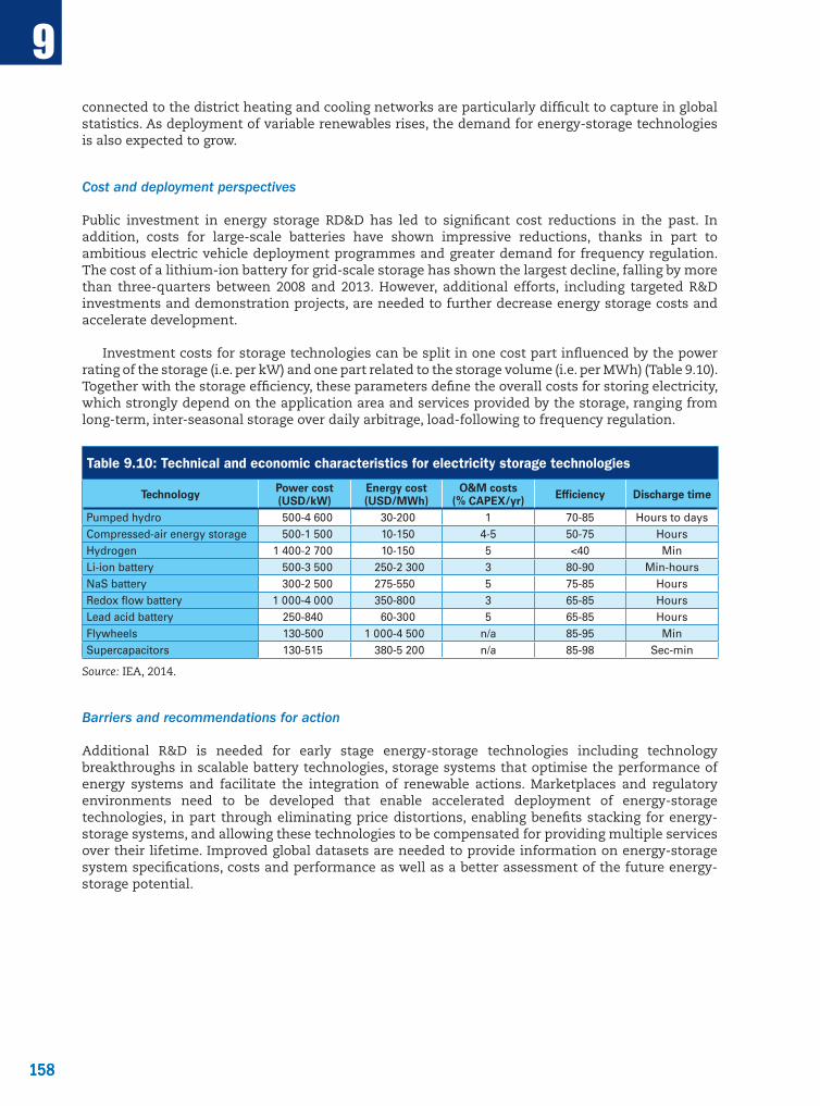
158

9

158

connected to the district heating and cooling networks are particularly difficult to capture in global statistics. As deployment of variable renewables rises, the demand for energy-storage technologies is also expected to grow.

Cost and deployment perspectives

Public investment in energy storage RD&D has led to significant cost reductions in the past. In addition, costs for large-scale batteries have shown impressive reductions, thanks in part to ambitious electric vehicle deployment programmes and greater demand for frequency regulation. The cost of a lithium-ion battery for grid-scale storage has shown the largest decline, falling by more than three-quarters between 2008 and 2013. However, additional efforts, including targeted R&D investments and demonstration projects, are needed to further decrease energy storage costs and accelerate development.

Investment costs for storage technologies can be split in one cost part influenced by the power rating of the storage (i.e. per kW) and one part related to the storage volume (i.e. per MWh) (Table 9.10). Together with the storage efficiency, these parameters define the overall costs for storing electricity, which strongly depend on the application area and services provided by the storage, ranging from long-term, inter-seasonal storage over daily arbitrage, load-following to frequency regulation.

Table 9.10: Technical and economic characteristics for electricity storage technologies

Technology Power cost (USD/kW)

Energy cost (USD/MWh)

O&M costs (% CAPEX/yr) Efficiency Discharge time

Pumped hydro 500-4 600 30-200 1 70-85 Hours to daysCompressed-air energy storage 500-1 500 10-150 4-5 50-75 HoursHydrogen 1 400-2 700 10-150 5 <40 MinLi-ion battery 500-3 500 250-2 300 3 80-90 Min-hoursNaS battery 300-2 500 275-550 5 75-85 HoursRedox flow battery 1 000-4 000 350-800 3 65-85 HoursLead acid battery 250-840 60-300 5 65-85 HoursFlywheels 130-500 1 000-4 500 n/a 85-95 MinSupercapacitors 130-515 380-5 200 n/a 85-98 Sec-min

Source: IEA, 2014.

Barriers and recommendations for action

Additional R&D is needed for early stage energy-storage technologies including technology breakthroughs in scalable battery technologies, storage systems that optimise the performance of energy systems and facilitate the integration of renewable actions. Marketplaces and regulatory environments need to be developed that enable accelerated deployment of energy-storage technologies, in part through eliminating price distortions, enabling benefits stacking for energy-storage systems, and allowing these technologies to be compensated for providing multiple services over their lifetime. Improved global datasets are needed to provide information on energy-storage system specifications, costs and performance as well as a better assessment of the future energy-storage potential.

159

9

159

9.11 Nuclear energy

Emerging nuclear technology overview

Emerging nuclear technologies in the 2015-2030 time frame include small modular reactors (SMRs), essentially based on the same technology as today’s generation III reactors (namely light water reactors) and prototypes of generation IV reactors, that could include very-high-temperature reactors (VHTR) for electricity and process heat applications, and liquid metal-cooled reactors such as sodium-cooled fast reactors (SFR) and lead-cooled fast reactors (LFR). Although initially developed and operated for electricity generation, all these advanced designs could also operate in some form of co-generation mode, with applications that include district heating, desalination, or process heat applications (including hydrogen production).

Cost and deployment perspectives

SMRs can target niche markets (for instance isolated regions or islands) and countries with small electricity grids that require baseload power. The replacement of coal-fired power plants by SMRs in the United States has also been identified as a potential market. There are wide-ranging projections of the installed SMR capacity by 2030. (See the forthcoming NEA study on the SMR market.) Today, two SMR-based plants are under construction, one in Argentina (CAREM reactor) and one in Russia (KLT-40s, a floating power plant). Because of their size, the specific per-MW costs of SMRs are likely to be higher (typically 50% to 100% higher per kWe for a single SMR plant) than those of large generation III reactors. However, economies of volume could compensate economies of scale if a sufficiently large number of identical SMR designs are built and replicated in factory assembly workshops. Lower overall investment costs and shorter construction times for SMRs could also facilitate the financing of such reactors compared to large nuclear plants at lower costs of capital. Variable costs (O&M and fuel costs) for SMRs most likely will remain higher than for large nuclear. In terms of total electricity generation costs, SMRs are expected at best to be on par with large nuclear if all the competitive advantages of SMRs are realised, including serial production, optimised supply chains and lower financing costs. Co-generation can also open additional revenue streams for the operators of SMRs, but the economics of non-electric applications and the associated business models are still to be established, and will also depend on the CO2 price of emissions from fossil-based heat processes that nuclear co-generation would replace.

Concerning generation IV technologies, a prototype high-temperature reactor (HTR-PM) is currently under construction in China – which may be considered a first step towards a VHTR. Japan and Korea are also actively pursuing development of this technology, targeting high-temperature process heat applications. Two recently built SFR prototypes are also expected to be connected to the grid in 2015: BN-800 in Russia and PFBR in India. Russia is currently developing a generation IV SFR prototype, BN-1200, with a net capacity of 1 200 MWe, although Russia has recently announced postponement of its construction. France is also developing a 600 MWe generation IV prototype called ASTRID to be in operation before 2030. Russia also plans to construct a first LFR prototype in that time frame. In terms of generation costs, generation IV technologies aim to be at least as competitive as generation III technologies (and will build on the enhanced safety levels of those technologies), though the additional complexity of these designs, the need to develop a specific supply chain for these reactors and the development of the associated fuel cycles will make this a challenging task. However, generation IV also provide additional benefits in terms of fuel utilisation and waste management (especially for fast neutron reactors) or in terms of high thermal efficiency, and potential for high temperature process heat application for HTRs – and this could represent an economic advantage over alternative technologies.

160

9

160

Table 9.11: Technical and economic characteristics for emerging nuclear technologies

Technology Typical size (MW)

Thermal efficiency

Projected costs in 2030

(USD/MWh)

Capacity in 2030 (GW)

Co-generation

SMR (LWR based) 20-300 33% 75-125 <20 District heating, desalination

Gen IV (HTR) 150-300 >45% 60-160 <1 Process heat, H2 production

Gen IV (SFR) 800-1 200 >40% 75-175 ~6 Process heat

Barriers and recommendations for action

In addition to the barriers that exist today for the deployment of large nuclear power plants, there are some specific barriers for new, sometimes unproven, reactor technologies. Licensing risks, for instance, are expected to be greater for emerging nuclear technologies, especially for generation IV reactors, since the first SMRs to be deployed will rely on proven light-water reactor technologies. For SMRs, the economics will depend on the number of units produced, and the learning rates from factory assembly. According to the IEA/NEA Technology Roadmap: Nuclear Energy (2015), the following recommendations can be made to support the further development and deployment of these innovative designs:

• To open up the market for SMRs, governments and industry should work together to identify target markets and accelerate the deployment of SMR prototypes in those markets, with the launch of construction projects (about five projects per design) needed to demonstrate the benefits of modular design and factory assembly (time frame 2015-2025).

• Governments should assess the long-term benefits of developing gen IV systems in terms of resource utilisation, cost, safety and waste management, and support R&D and prototype development of fast neutron reactor gen IV prototypes (time frame 2015-2030).

• Public-private partnerships need to be put in place between governments and industry in order to develop demonstration projects for nuclear co-generation in the area of desalination or hydrogen production (time frame 2030).

9.12 Concluding remarks

In addition to the discussion of new nuclear power plants (NPPs), long-term operation (LTO), also known as “lifetime extension” of operating nuclear power plants, should also be discussed. While not an emerging technology in the strict sense, since the technologies involved are well known, this constitutes an emerging issue in the nuclear power industry. In some parts of the world (United States, Canada, Europe, Russia, Japan) a large number of existing nuclear plants are reaching their initial design lifetime (30 or 40 years). Therefore, one could anticipate that, in the coming two decades, extensive refurbishment and safety upgrade programmes will be started, if economically justified and accepted by the national safety authorities. Such extensive refurbishment and upgrade programmes cannot be compared with routine maintenance. They are more costly and may therefore be considered and analysed as a major capital investment associated with a “20-year lifetime” nuclear power plant. Some examples of capital investment costs necessary for long-term operation can be found in NEA (2012) and are summarised in Table 9.11.

161

9

161

Table 9.12: Cost summary of LTO and refurbishment programmes in selected countries

Country Specific investment in LTO Co-generation

Belgium USD2010 650/kWe Including ~11% increase due to post-Fukushima measures.

France USD2010 1 090/kWeIncluding all investments from 2011 to 2025: maintenance, refurbishment, safety upgrades, performance improvement; and ~10% increase due to post-Fukushima measures.

Hungary USD2010 740-792/kWe Including 10-17% increase due to post-Fukushima measures.Korea USD 500/kWe Including ~10% increase due to post-Fukushima measures.

Switzerland USD2010 490-650/kWeSpecific future investment in NPP refurbishment and maintenance (approximately the double of the specific LTO investment) is USD2010 980 1 300/kWe.

United States About USD2010 750/kWe Electric Power Research Institute (EPRI) survey data and current spending on capital improvement.

Non-OECD countriesRussia About USD2010 485/kWe Data for Novovoronezh 5 unit (first series of VVER-1000: V-187).Ukraine About USD 300-500/kWe Public statements by Energoatom and Ukrainian prime minister.

Such programmes are usually performed over a few years during (extended) outages. This means that the “duration” of these programmes is an important factor influencing the overall cost. Starting from these “investment costs” and adding the O&M costs, fuel costs, and even extra decommissioning fees, one could then calculate the LCOE produced by a nuclear plant under long-term operation (lifetime extension) conditions. Such a calculation has been done for the European Commission by D’haeseleer (2013), assuming the following (these calculations of the LCOE of lifetime extension are based on future cash flows and do not take into account the cost or value of past investments):

Overnight refurbishment cost (ORC): 400, 600 and EUR2012 850/MWe

Refurbishment period: 2 years, spending 50% of the ORC each year

Capacity factor after refurbishment: 85%

Lifetime extension: 20 years

Decommissioning fee: 15% of the ORC

Fuel costs (similar to a new build): EUR2012 6/MWh

O&M costs (similar to a new build): EUR2012 10/MWh

Discount rate: 5% and 10%

Sample calculation results are

With an ORC of EUR 400 (ref – 33%) LCOELTO(5%)= EUR 21/MWh, LCOELTO(10%)= EUR 23/MWh

With an ORC of EUR 600 (reference) LCOELTO(5%)= EUR 23/MWh and LCOELTO(10%)= EUR 26/MWh

With an ORC of EUR 600 and EUR 850 (ref + 42%) LCOELTO(5%)= EUR 26/MWh and LCOELTO(10%)= EUR 30/MWh

Clearly, the LCOE for long-term operation (lifetime extension) of an existing nuclear plant may compare favourably with other electricity generation sources and should deserve attention. This could also be the case for extensive refurbishment (lifetime extension) programmes for other technologies, where applicable. Therefore, these estimations could be considered in the next edition of this report.

162

9

162

References

Crown Estate (2012), Offshore Wind Cost Reduction: Pathways Study, The Crown Estate, London, www.thecrownestate.co.uk/media/305094/offshore-wind-cost-reduction-pathways-study.pdf.

Decourt, B., et al. (2014), “Hydrogen based energy conversion. More than storage: System flexibility”, SBC Energy Institute, Paris.

D’haeseleer, William D. (2013), “Synthesis on the Economics of Nuclear Energy”, report for the European Commission, www.mech.kuleuven.be/en/tme/research/energy_environment/Pdf/wpen2013-14.pdf.

IEA (2014), Energy Technology Perspectives 2014, OECD, Paris.

IEA/NEA (2015), Technology Roadmap: Nuclear Energy (2015 edition), OECD, Paris, www.oecd-nea.org/pub/techroadmap/techroadmap-2015.pdf.

NEA (2012), The Economics of Long-term Operation of Nuclear Power Plants, OECD, Paris.

NEA (2015), Nuclear New Build: Insights into Financing and Project Management, OECD, Paris.

NEA (2015b), Small Modular Reactors: Market Potential for New-term Deployment (forthcoming), OECD, Paris.

NETL (2013), “Assessment of the Distributed Generation Market Potential for Solid Oxide Fuel Cells”, September, DOE/NETL- 342/093013, National Energy Technology Laboratory.

US DOE (2014), 2013 Fuel Cell Technologies Market Report, Fuel Cell Technologies Office, November, Department of Energy, Washington DC.

163

10

163

Chapter

The system cost and system value of electricity generation

10.1 Going beyond generation costs

Generation cost for various technology options is most commonly expressed in energy terms and labelled levelised cost of electricity (LCOE). LCOE is calculated by summing all plant-level costs (investments, fuel, emissions, operation and maintenance, dismantling, etc.) and dividing them by the amount of electricity the plant will produce, after an appropriate discounting. The LCOE represents the average lifetime cost for providing a unit of output (MWh) for a given capacity factor, often the average capacity factor achievable by the power plant or a common value typical of baseload plants. This simple metric allows for a straightforward comparison of technologies that have a different size, different lifetimes and a different profile of expenditures.

However, LCOE as a measure is blind to the when, where and how of power generation. The when refers to the temporal profile of power generation that can be achieved, the where refers to the location of the power plant, and the how refers to the technical characteristics of the equipment used. The LCOE considers only direct input costs and implicitly assumes that the electricity generated from different sources has the same economic value. Whenever technologies differ in the when, where and how of their generation, a comparison based on LCOE does not capture the full picture and thus may be misleading.

Several studies have shown how the LCOE metric fails to take into account the differences in the production profile of variable renewable energy (VRE) and dispatchable technologies, and the associated market value of the electricity that they supply (Joskow, 2011; Mills and Wiser, 2013; and Hirth, 2013). Also for dispatchable plants, a simple comparison of LCOE alone gives little information with respect to their importance and role in the electricity system. For example, a comparison between a dispatchable baseload technology and a hydro reservoir based on the LCOE alone has little practical sense since it does not capture the difference in value of the electricity produced by the two plants: the hydropower plant will optimise its scarce water resources to produce primarily in periods of scarcity, when the market price is comparably high. When comparing LCOEs, it is impossible to infer which would be the optimal deployment of the two technologies. Similarly, a comparison between the LCOE of a peaking and a baseload generator is not sufficient to infer why one should build a mix of the two technologies. Assuming that both technologies run at a high capacity factor, the peaking plant would appear uneconomic. Conversely, assuming a very low capacity factor would make the baseload power plant appear excessively expensive. To get the full picture, one would need to compare the two technologies over a continuous range of capacity factors.1

1. Such a comparison can be done by using load-duration curves, which order electricity demand from highest to lowest demand levels. This allows deriving the optimal power plant mix to meet a given demand; see NEA (2012) and IEA (2014) for a more detailed explanation.

164

10

164

A second weakness of the LCOE is that it is a measure of economic cost for a particular generation technology taken in isolation, at the level of the plant itself. Thus it does not take into account the interactions between that power plant and the rest of the electricity system and the implications of its integration into the system.

The rise of VRE technologies to a mass scale has added to the challenges associated with comparisons based on LCOE alone. VRE technology carries the temporal and spatial imprint of its resource, is more modular than conventional technologies and is typically not electro-mechanically coupled with the grid but uses power electronics. All these factors affect the possible when, where and how of power generation from VRE (IEA, 2014). This has raised questions about the economic value of VRE for power systems since the onset of VRE deployment (Grubb, 1991). To understand the economic implications of VRE deployment, it is critical to go beyond generation costs expressed in LCOE.

The portfolio value of renewables

Common approaches to power system cost analysis often disregard the fact that system parameters, such as fuel costs, are highly uncertain. Consequently, important risks from the end-user (ratepayer) perspective might be left out. Arguably, a whole series of risks – e.g. construction risks, technology risks, etc. – can be reflected in the LCOE framework through the weighted average cost of capital of the investment. However, the risks affecting the running costs, in particular the fuel cost risks (and the CO2 price risks), are not part of such an analysis, as the bulk of these risks can usually be passed through to the final customers. Energy security, which the IEA defines as “the uninterrupted availability of energy sources at an affordable price”, is thus not necessarily maximised with respect to the provision of electricity with these common methods.

Over half a century ago, Harry Markowitz first established the mean-variance portfolio theory. He showed that an investor can reduce portfolio risks in holding combinations of assets, of which returns are not perfectly cor-related. Furthermore, he showed that introducing low-return risk-free assets in the portfolio always increases the efficiency of the portfolio, further reducing the risk for a given return, or, perhaps counter-intuitively, increasing the return for a given level of risk. The mean-variance portfolio can be readily transferred to the analysis of generating technology portfolios (see e.g. Awerbuch and Berger, 2003). “Return” here simply stands for the inverse of the LCOE, so that “low return” stands for “high cost”. A diversified portfolio of non-perfectly correlated “returns” would stand for a mix of coal, gas and nuclear. With respect to the risks that are not borne by the investors but by the ratepayers, i.e. the fuel (and CO2) risks, renewables (except for bioenergy) are risk-free. This could also apply to nuclear power, although it is not entirely immune from fuel risks.

In short: higher costs but fuel risk-free renewables and, to some extent, nuclear power, if introduced in the right proportion in a generating technology portfolio, allow for a more efficient portfolio, reducing the risk for a given aver-age LCOE of a mix of technologies. Or, put differently, will lead to lower costs at a given level of risk.

The mean-variance portfolio only represents the simplest risk/return analysis. Criticisms have been raised, some being fully relevant when the tool is transposed to generating portfolio analysis. For example, risk is only analysed through the prism of volatility, for which the past provides the basis to assess the future. The energy world knows very well that energy security risks, or technology risks, have many other dimensions, such as physical sup-ply interruptions, or accidents; they need to be assessed with different tools, such as probability risk assessments, where a possible chain of events and their causal relationships need to be considered and quantified.

Furthermore, the mean variance portfolio analysis only scratches the surface of the risk probabilities in con-sidering mean and variance but no “higher moments” of probability distribution, skewness and kurtosis. In other words, the analysis works as if fuel cost volatility distributions were “normal”, or Gaussian. In reality they are not, they are skewed towards higher fuel costs (the price of a fuel can increase by 100% but never decreases by 100%). They also exhibit fat tails, that is, extremely high price events, although rare, are more frequent than a normal probability distribution would suggest. Another limitation arises from the dependence of LCOE to capacity factors. Mean-variance portfolio analyses take deterministic assumptions relative to capacity factors, thereby ignoring the changes in merit order and load duration curves as fuel costs and carbon prices vary.

For all these reasons, more powerful tools, such as Monte-Carlo simulations, may be needed to perform more realistic risk/return analyses of power generating portfolios and reveal the true value and optimal shares of risk-free assets in such portfolios (see e.g. Vithayasrichareon and MacGill, 2012).

Such analyses would go beyond the scope of the present publication. However, it is important to stress that, while a broad analysis of system costs arising from the variability and uncertainty of some renewable energy technologies may modify the perception of their value, so would an analysis of their value in any given generating portfolio in consideration of the variability and uncertainty affecting the fuel costs and CO2 prices – though most likely with an opposite sign.

165

10

165

The analysis of system effects takes an intermediate position between generation costs of a technology captured by LCOE and a full cost-benefit calculation of the deployment of a generation technology. Such a comprehensive assessment would factor in environmental aspects or effects on the wider economy. An additional consideration is the stochastic nature of some of the cost assumptions used in an analysis of system costs, such as fuel price volatility. While a detailed stochastic analysis is beyond the scope of this chapter, some general considerations can be found in the box above.

10.2 System effects

The concept of system effects has been introduced to describe and take into account the interactions between different generation technologies and the infrastructure constituting the power system, and to capture the impacts of the introduction of each technology on the whole system. System effect analysis also provides a framework for characterising the contribution of a given generation technology to the overall power system.

Taking the examples provided above, it is the interaction between the properties of all available generation technologies and power demand that determine the optimal mix. This interaction can only be understood by combining information across different components of the power system – it is a system effect. Along the same lines, the interaction of VRE and other system components can be understood in terms of system effects. However, owing to the intrinsic characteristics of the VRE, their integration in power systems has more pronounced effects on the other components of the system and present novel challenges and opportunities.

The system effects associated with VRE are frequently categorised according to the underlying properties of VRE:

• The economic influence of the variability in output is captured by profile costs (Hirth, 2015; and Ueckerdt et al., 2013b). Profile costs include all effects related to the temporal pattern of VRE generation, assuming that output is fully predictable. The essence of profile cost is the auto-correlation of the output of a VRE plant with that of other plants of the same technology; a given VRE generator is more likely to generate when other VRE plants are also generating. Especially at high penetration levels, VRE generators tend to produce disproportionally more power at lower electricity prices. Profile costs include also variability at short-time scales, which requires a more flexible residual system that can imply a higher ramping and cycling burden to other plants, thus increasing generation costs.2 Profile costs include also the effects associated with the frequently low capacity credit of VRE.3

• Uncertainty of output (forecast errors, plant failures) is quantified as balancing costs. Because of the uncertainty of VRE production, it may be necessary to change power plant schedules more frequently and closer to real time. In addition, balancing forecast errors may require carrying a higher amount of reserves on the system. All this may lead to increased costs for the system. For practical reasons, the variability of VRE within the scheduling interval of power systems (one hour and below) is sometimes also accounted for in balancing costs. Unless stated otherwise, balancing costs are understood to include only the impacts related to uncertainty.

2. These costs are apparent even under perfect foresight of VRE production.

3. Profile costs avoid a number of analytical shortcomings associated with so-called capacity costs, which aim at extracting additional costs associated solely with the frequently low capacity credit of VRE. For a discussion of these shortcomings, see Hirth, Ueckerdta and Edenhofera (2015).

166

10

166

• The effects on the transmission and distribution grid related to location constraints of the VRE (grid effects). Location constraints and associated grid costs are not unique to VRE. Accommodating VRE may require additional investments in the transport and distribution infrastructure and, more generally, a different structure of the grid. In general, grid-related costs tend to increase as a result of connecting distant power plants or accommodating distributed resources. Transmission losses also tend to increase when electricity has to be moved over longer distances. In some specific cases, however, grid-related cost may fall as a result of VRE deployment.

Although common, the above categorisation may not be fully exhaustive. For example, the fact that VRE are non-synchronous sources of generation may become economically significant at high shares, at least in smaller power systems. One could thus consider adding this category to the above list. To the knowledge of the authors, there has not been a systematic attempt to quantify the economic influence of this property and it will thus not be discussed further.

Connection costs, i.e. the cost of connecting the power plant to the nearest connecting point of the existing transmission grid, are sometimes integrated within the system costs (NEA, 2012) and more often not considered as system costs and, implicitly, included into the LCOE assessment. The difficulty in the categorisation of these costs lies in the fact that connection costs are sometimes borne by the power plant developer and are thus fully internalised, and sometimes borne by the transmission grid operator and thus become part of the cost for the whole electricity system. In the former case, the associated need for grid connection would already be included under the direct costs of the power plant and hence not constitute a system effect. However, it is important that connection costs be accounted for in an economic analysis and appear as a component either of the plant-level costs or of the system costs. In the following discussion, grid connection costs are not explicitly considered part of system costs.4

An additional complication may arise when defining what constitutes a system effect within one of the above three categories. For example, curtailment of VRE can be seen as increasing the LCOE of a given technology or they may be accounted for as a system effect related to the profile of VRE. Either way of accounting for curtailment effects is possible, but consistency is crucial.

Segmentation into the above three categories can be useful to derive an estimate of the economic relevance of each impact group. Segmentation is often necessary because existing power system models can only capture some impact groups at once, i.e. they may specialise in assessing grid impacts, balancing impacts or profile impacts.

However, the different categories are not independent of one another. For example, increased investment in grid infrastructure may contribute to smoothing the variability of VRE at the system level, and thus reduce balancing and profile impacts. Similarly, a longer-term adaptation of the generation mix towards more flexible units will lower balancing costs, but may have consequences with regard to profile costs. A rigorous decomposition into the above three categories is thus generally not possible. Because the different integration cost categories are not independent of one another, caution is needed when adding up components, in particular if they have been obtained from different modelling exercises.

These caveats notwithstanding, the above categorisation remains useful to analyse system effects. However, it should also be clear that any assessment of system effects is a complex undertaking, subject to ad hoc assumptions. As such, results always need to be seen in the context of the methodology used to derive them.

4. A discussion of different levels of grid connection costs can be found in ENTSO-E (2015).

167

10

167

10.3 System cost and system value

It is important to note that system costs are not direct costs in a strict accounting sense. If one imagines receiving a “bill” for the entire power system, it is straightforward to isolate, for example, fuel costs as a separate line item. For system costs, however, such a separation does not exist a priori. This is a direct consequence of their underlying nature: because they depend on the interplay of the various components of the system, they cannot be easily sorted out and a straightforward attribution to each system component is difficult. Instead, they need to be defined and constructed by comparing different scenarios. To use once again the example of receiving a “bill” for the power system, one could only identify system costs by comparing two bills, corresponding to two different scenarios; one bill corresponding to a reference benchmark case and the other corresponding to the technology under study.

Adding VRE to this bill will trigger two different groups of economic effects that will be reflected in the bill:

• Some costs increase. This includes the cost of VRE deployment itself (LCOE). Other additional costs are the costs for additional grid infrastructure or an increased cost for providing balancing services (i.e.  increased costs of cycling conventional power plant and additional reserve requirements). This group can be termed additional costs.

• Some costs decrease. Depending on circumstances, this includes reduced fuel costs, reduced carbon dioxide and other pollutant emissions costs, reduced need for other generation capacity and reduced need for grid and reduced losses. This group can be termed benefits or avoided costs.

Two additional points should be clearly identified in order to fully understand the nature of system effects. While some costs and benefits of VRE deployment for the system are immediately visible, some others become apparent only in a much longer time frame. The time aspect is therefore of a great importance for the assessment of the costs and benefits of deploying a new technology (this aspect is treated in greater detail in Section 10.4).

A second point is that the two above categories cannot be strictly separated and the same technology may lead to different outcomes depending on the penetration level. For example, at low shares, solar PV may contribute to shaving midday peaks, thus reducing the need for plant cycling. Meanwhile, at higher shares it may create a midday net load valley, which increases cycling needs and balancing requirements.

Two analytical approaches have been adopted in the literature to quantify the economic impacts of variable renewable energy: the system cost and system value approaches. Both approaches rely on sophisticated computer software that tries to accurately calculate the cost of power system operation and investments under different scenarios.

In very broad terms, the system value approach analyses the economic benefits of the deployment of a given VRE technology for the system. Net benefits (system value) are assessed as the difference between the total costs of the initial system (without VRE) and that of the residual system, after the introduction of VRE; initially, this assessment does not consider the costs for the deployment and operations of VRE in this first step. In a second step, the direct cost of the technology (LCOE) is then related to its net benefit for the rest of the power system (system value). This approach thus answers the question whether adding a specific technology to the system brings more benefits (system value) than costs (LCOE). In the literature, calculations often step through different penetration levels, and it is possible to derive the marginal benefit from the deployment of an additional increment of output; it is then possible to derive the optimal level of deployment for a VRE technology by equating its marginal benefits to the cost of adding the marginal unit.

The system cost approach aims at comparing two or more different technologies with each other. System costs are assessed by comparing the technology under study (say wind) with an explicit

168

10

168

benchmark technology which provides the same amount of electricity (say a generator with constant output). System costs are defined as the difference in cost for the residual system between two scenarios. If the technology under consideration brings less net benefits to the system than the benchmark, it is defined to have a system cost. The costs (positive or negative) obtained in such way are then added to the plant-level LCOE of each technology, often as a function of the penetration rate; the system-level LCOE (the sum of LCOE and system costs) allows for a direct and straightforward comparison across technologies. A graphical illustration of the two approaches is provided in Figure 10.1.

Figure 10.1: Illustration of system costs, system value and system cost approaches

Averageelectricity price

Pro�lecosts

Balancingcosts

Grid-relatedcosts

Residual Wind market value

E�ect of timing

E�ect of forecast errors

E�ect of location Interaction

e�ect

Integrationcosts

System value approach

EUR/

MW

h

EUR/

MW

h

Integrationcosts

Short-termintegrationcosts

Generationcosts

LCOE Pro�lecosts

Balancingcosts

Gridcosts

Short-termsystemLCOE

Flexibilityoptions

SystemLCOE

System cost approach

In synthesis, system value quantifies system effects by comparing a scenario with and without a given technology (wind in the example). System cost quantifies system effects by comparing a scenario using a given technology or a benchmark providing the same share of generation. Ultimately, both approaches convey the same information; however, they differ in the way this information is expressed.

Choice of benchmark technology

The definition of system costs intrinsically requires a comparison between two different systems. Moreover, it requires making a choice of the reference benchmark technology. These choices will influence the result of the system cost calculation.

Choosing a benchmark that leads to very high savings in the residual system will yield higher system costs for other technologies. Conversely, choosing a benchmark with lower savings leads to lower absolute numbers for system costs. Using the example in Figure 10.2, the avoided cost for the residual system is USD 2.5 billion in the benchmark case. Choosing a different benchmark with savings of, say, USD 3 billion, leads to system costs of USD 1 billion instead of USD 0.5 billion. This result may appear surprising. How can it be that system costs double simply by choosing a different benchmark technology? This property reflects the fact that system costs are not a direct cost in an accounting sense. They reflect the opportunity cost of building a given technology rather than the benchmark.

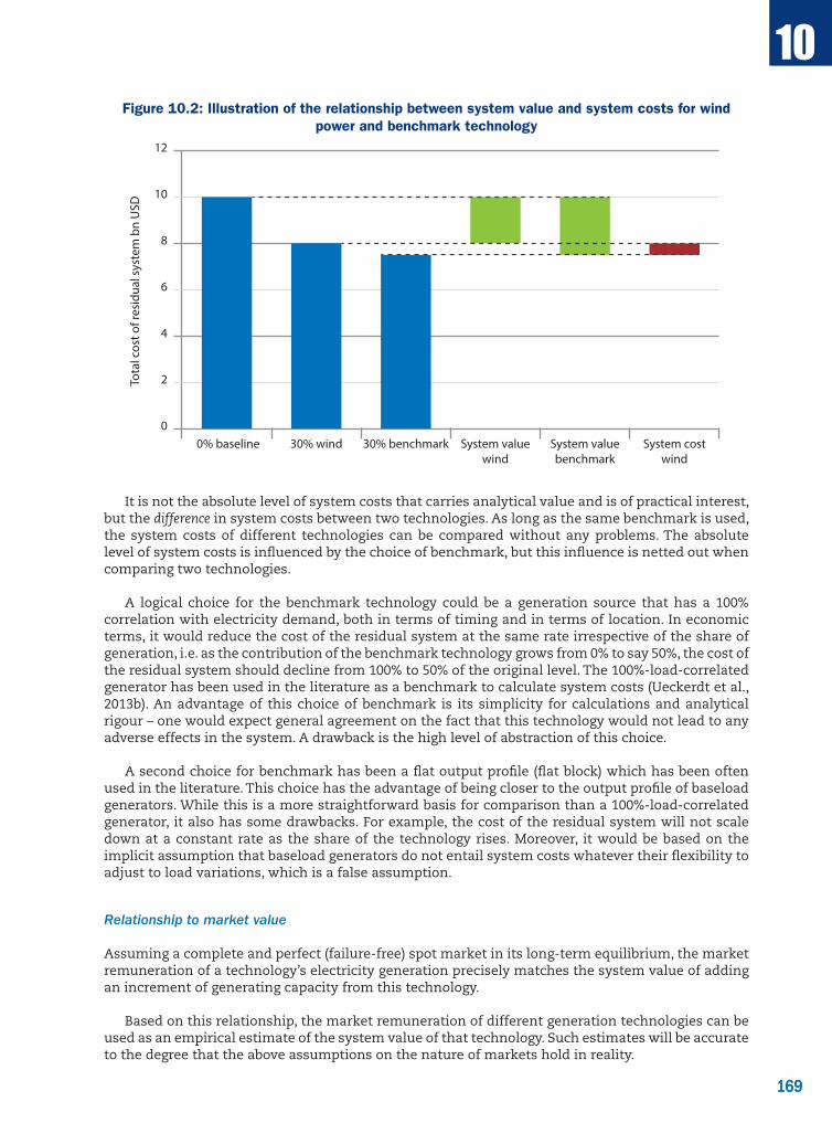
169

10

169

Figure 10.2: Illustration of the relationship between system value and system costs for wind power and benchmark technology

0

2

4

6

8

10

12

System costwind

System valuebenchmark

System valuewind

30% benchmark30% wind 0% baseline

Tota

l cos

t of r

esid

ual s

yste

m b

n U

SD

It is not the absolute level of system costs that carries analytical value and is of practical interest, but the difference in system costs between two technologies. As long as the same benchmark is used, the system costs of different technologies can be compared without any problems. The absolute level of system costs is influenced by the choice of benchmark, but this influence is netted out when comparing two technologies.

A logical choice for the benchmark technology could be a generation source that has a 100% correlation with electricity demand, both in terms of timing and in terms of location. In economic terms, it would reduce the cost of the residual system at the same rate irrespective of the share of generation, i.e. as the contribution of the benchmark technology grows from 0% to say 50%, the cost of the residual system should decline from 100% to 50% of the original level. The 100%-load-correlated generator has been used in the literature as a benchmark to calculate system costs (Ueckerdt et al., 2013b). An advantage of this choice of benchmark is its simplicity for calculations and analytical rigour – one would expect general agreement on the fact that this technology would not lead to any adverse effects in the system. A drawback is the high level of abstraction of this choice.

A second choice for benchmark has been a flat output profile (flat block) which has been often used in the literature. This choice has the advantage of being closer to the output profile of baseload generators. While this is a more straightforward basis for comparison than a 100%-load-correlated generator, it also has some drawbacks. For example, the cost of the residual system will not scale down at a constant rate as the share of the technology rises. Moreover, it would be based on the implicit assumption that baseload generators do not entail system costs whatever their flexibility to adjust to load variations, which is a false assumption.

Relationship to market value

Assuming a complete and perfect (failure-free) spot market in its long-term equilibrium, the market remuneration of a technology’s electricity generation precisely matches the system value of adding an increment of generating capacity from this technology.

Based on this relationship, the market remuneration of different generation technologies can be used as an empirical estimate of the system value of that technology. Such estimates will be accurate to the degree that the above assumptions on the nature of markets hold in reality.

170

10

170

Comparing the market remuneration of two different technologies and using one of them as a benchmark also allows for the calculation of system costs from market data. This has been done in particular to compute estimates for profile costs (Fripp et al., 2008; Joskow, 2011; Hirth, 2013 and 2015). For specific types of benchmarks, the market remuneration can be calculated in a very simple manner. A flat-block generator will receive a remuneration corresponding to the simple average of the market price across time (system base price). A 100%-load-correlated generator will receive the demand-weighted average market price.

An alternative way to express system costs in this case is to divide the specific remuneration of a given technology (e.g. wind) by the system base price. This ratio is called value factor (relative price). Consequently, system costs (calculated against the flat-block benchmark) can be calculated from the value factor by multiplying it with the system base price.

The relationship between system costs and market value has another important consequence: the market remuneration of different technologies already internalises part of the system costs of the respective technologies.5

10.4 Long-term and short-term effects

An assessment of overall economic costs and benefits arising from the introduction of new generating capacity in the system, and of the impacts on the operations and economic profitability of existing assets, depends strongly upon the time horizon chosen.

The structure of the electricity generation mix, as well as the electricity demand pattern, is quite inelastic in the short term: existing power plants have long lifetimes and building new capacity and transmission infrastructure may require a considerable lead time as well as significant upfront investments. In other terms, electricity systems are locked in with their existing generation mix and infrastructure, and cannot quickly adapt them to changing market conditions. In the long term, instead, utilities can adapt their generation mix and infrastructure to new market conditions which result from changes in demand, expected fuel price level as well as the emergency and introduction of new technologies into the generation mix.

To illustrate these effects, it is useful to introduce two schematic and inevitably simplified scenarios, based on a short-term and a long-term perspective. In the short-term scenario, new generation is introduced in the electricity system almost instantaneously, and without being anticipated by the market. In this perspective, the physical assets of the power system cannot be changed and investments already occurred are sunk. In the long-term scenario, the analysis is situated in the future when all the market participants had the possibility to adapt their generation capacities and infrastructure to new market conditions. In other words, the electricity system is considered as a greenfield, and the whole generation stock and infrastructure can be replaced and re-optimised.

The two scenarios will inevitably lead to different estimates of system costs and of the system value of introducing a new technology such as VRE. This approach could be interpreted simply as providing upper and lower limits for a more realistic assessment of system cost, but it also helps to underline and understand some important phenomena arising from the integration of a new technology into the system and to provide useful information to policy analysts.

5. There are a number of real-life effects where there can be externalities nevertheless. In an energy-only market, market agents will price in start-up, ramping and part-load efficiency costs into their bids. This can raise the market value of technologies that increase the cycling burden of the system. In this case, the system value of the technology will be lower than its market value.

171

10

171

By how much the “true” system costs will differ in a more realistic situation depends mainly on three factors: the evolution of electricity demand, the system’s capital turnover rate relative to the speed of deployment of the new technology, and the degree to which existing and available assets complement the new entrants. For example, if VRE are introduced very slowly relative to the natural turnover rate of the power system or relative to the change in electricity demand, the system could remain continuously well adapted during the transformation process and system costs stay at a minimum level (long-term costs). Instead, if VRE are rapidly introduced to a power system with a lower turnover rate and with a flat demand, system costs will be higher and close to those of a short-term perspective.

Also, the structure of the existing generation resources will have a significant impact. Where VRE are added to a system that provides a good match in terms of existing technologies, short-term costs will be only slightly higher than long-term costs.

Finally, the number of adaptation options considered can have a significant impact on system cost assessments (IEA, 2014). The possibility to develop additional flexible resources in an economic manner is an essential driver to reduce system costs both in the short term and in the long term; system cost will be much less in a system which has sufficient flexible resources existing or economically available, than in a system with little opportunity to develop flexible resources.

Short-term impacts on existing assets and long-term effects on the generation mix following the introduction of large shares of VRE

The introduction of significant shares of VRE is currently the most relevant application for system effect analysis in the energy sector.

The benefits that the introduction of a new technology such as VRE may bring to the electricity system depend upon the possibility of the system itself to adapt and thus are a function of the time horizon chosen.

In the short term, the load structure and the physical assets of the system cannot be changed, and only operations can be adapted. From a system viewpoint, the economic benefits of introducing new capacity are limited to variable cost savings (fuel, carbon and variable O&M costs) of the technology displaced. In this time frame, the cost for the system includes the investment costs for the new capacity, plus higher balancing costs and grid-related investments.

In the medium term, power plants can be decommissioned or mothballed, and the power generation can adjust to be more flexible. Also, investment in new plants that would have been otherwise needed can be deferred or cancelled. The economic benefits would thus include also the fixed O&M of the decommissioned plants and the investment costs of the plants no longer needed. Balancing costs and grid-related costs can be reduced in comparison to those in the short term.

In the long term, the system has the time to adapt to the introduction of new technology and the full benefits provided are available. A more detailed discussion of the level of system adaptation as a function of the time horizon may be found in Ueckerdt (2013a).

Adding large shares of VRE to the generation mix can have an important impact on the operations and on the revenues of existing power plants, as well as on the volatility and average level of electricity prices and on carbon emissions from electricity generation. Many of these effects are transitory and tend to gradually disappear with the adaptation of the electricity system to new capacity. However, in the long term, the introduction of VRE can have significant effects on the optimal structure of the generation mix, with a shift towards more peaking and mid-merit plants and a corresponding decrease in baseload generation. Depending on the relative cost of generation options, this structural shift in the generation mix can have an important impact on the cost for providing the residual load.

172

10

172

These effects derive from two characteristics intrinsic of variable renewable technologies:

• Low short-run generation costs; once built, variable renewables are likely to be among the first technologies in the merit order.

• The variability of the collective output of wind and solar PV, which itself results from the auto-correlation of their production: it is likely that a given wind (or solar PV) power plant is producing when other wind (or solar) plants in the system are also producing.

Many studies have shown that, in the short term, an addition of new VRE capacity into the system will cause two different effects on electricity markets:

• Reduction in the capacity factor of existing generators, mostly those with highest short-run costs (transitory utilisation or compression effect).

• Reduction on the electricity market price when VRE are generating (merit order effect).

An illustration of the capacity factor losses experienced by existing dispatchable plants following the introduction of a significant share of VRE is provided in Figure 10.3 (NEA, 2012). In this example, an “optimal” generation mix has been established to minimise the generation costs for a yearly load duration curve (the black curve in the illustration) in the absence of VRE generation. Then a given amount of wind generation is added to the system, providing 30% of the total electricity consumption. Because of the lower marginal costs of wind, the residual load curve seen by dispatchable technologies is shifted to a lower level (grey curve). Figure 10.3 illustrates the short-term effects of introducing wind power in the system, while Figure 10.5 shows the long-term effects, when the system has adapted. In Figure 10.3 the electricity generated by wind can be visualised by the darker area between the two lines representing the yearly demand load and the residual demand load. In absolute terms, low marginal cost wind substitutes mainly baseload and mid-load technologies (nuclear and coal in this example). However, when expressed in relation to the total output, peaking plants are the most penalised in the short term, with a significant reduction of their maximal utilisation time and of overall electricity production. At the penetration level considered in this example, the short-term production losses for peaking plants can reach up to 80% of the level expected in the absence of VRE.

Figure 10.3: Short-term reduction in capacity factor for existing power plants after the introduction of wind power

Gas (OCGT): Lost loadGas (CCGT): Lost loadCoal: Lost loadNuclear: Lost loadYearly loadResidual load

0

10

20

30

40

50

60

70

80

90

100

0 1 000 2 000 3 000 4 000 5 000 6 000 7 000 8 000

Pow

er (G

W)

Utilisation time (hours/year)

Gas (CCGT): lost loadGas (OCGT): lost load

Coal: lost loadNuclear: lost loadYearly loadResidual load

Note: based on load data and wind profile for France 2011. Wind generation scaled to a penetration of 30%; scaling may overestimate the impact of variability. For illustration only.

173

10

173

A graphical illustration of the merit order effect is provided in Figure 10.4. Because of the infeed of low marginal cost electricity, the supply curve shifts to the right, pushing plants with higher marginal costs out of the market. The electricity market can thus experience a decrease of the number of hours in which peak and mid-load technologies are marginal, which results in lower spot and average electricity prices and in a reduction of infra-marginal rent for base- and medium-load technologies. The merit-order effect is very strong if the merit-order curve is steep. Conversely, a flat merit-order curve will indicate little or no merit-order effect.

Figure 10.4: Illustration of the merit order effect

0

20

40

60

80

100

120

140

160

180

0 2 4 6 8 10 12 14 16 18 20 22 24 26 28 30 32 34 36 38 40 42 44 46 48 50 52 54 56 58 60 62 64 66 68 70 72 74 76

Elec

tric

ity p

rice

(USD

/MW

h)

Capacity (GW)

OilGas GTGas CCGTCoalBioenergyLigniteNuclearDemand

P1

0

20

40

60

80

100

120

140

160

180

0 2 4 6 8 10 12 14 16 18 20 22 24 26 28 30 32 34 36 38 40 42 44 46 48 50 52 54 56 58 60 62 64 66 68 70 72 74 76

Elec

tric

ity p

rices

(USD

/MW

h)

Capacity (GW)

Original merit-order

Shifted merit-order

Demand

P1

P2

Note: CCGT = combined-cycle gas turbine; GT = gas turbine; GW = gigawatt; P1 = price without additional generation; P2 = price with additional generation.

Source: Schaber, 2014.

The combination of reduced capacity factors and lower average electricity prices can have a severe impact on the revenues and thus profitability of existing power generation plants. This phenomenon affects all existing power plants but is more significant for peak- and medium-load generation. The merit-order effect is also important for the economics of VRE itself: market prices are lowered only when VRE is generating. This means that the market value of VRE technologies, i.e. the average price received on the power market, can experience an even stronger reduction than average market price, in particular at high shares (see Hirth, 2013; Mills and Wiser, 2012).

174

10

174

The presence of specific policies designed to support the deployment of renewable technologies, such as feed-in tariffs, feed-in premiums, tradable green certificates or production-based tax incentives, could contribute to the occurrence of negative power prices in the electricity markets and thus increase the revenue losses of existing generation. Based purely on plant economics, VRE generators would be expected to bid no lower than at a very low, positive price, reflecting their very low short-run cost. They would not be expected to bid below zero. However, support policies which contain a performance-based element may create an incentive for VRE plant owners to bid below their short-run costs, because they receive revenues on top of achieved market prices. Hence, bids may be below zero (minimum bids are likely to equal short-run cost minus the value of support payments). Other technologies may bid at prices well below marginal short-run costs or negative costs, as a result of “must-run” levels that would allow for a rapid ramping-up when the VRE generators fade – for example PV electricity when the sun sets. This effect could be reinforced by “take-or-pay” fuel contracts, for example for gas plants. Depending on the policy context, VRE generators may also enjoy priority dispatch. Where VRE generators have priority dispatch, their operation can run independently of any market price signal. This can lead to more pronounced negative prices (Nicolosi, 2012). However, negative price signals can also prove useful. If well implemented, they deliver a signal to all generators that increased flexibility is necessary. Negative price signals are thought, for example, to have encouraged the reduction of must-run levels of coal plants in Denmark.

If the economics of peak- and mid-merit plants are challenged mostly by rapid VRE additions in the short and medium term, the impacts in the long term affect mainly baseload plants. Adding low marginal-cost electricity from VRE creates a new residual load curve that must be satisfied by an optimal combination of system resources. Increased grid capacities, demand-side response and storage can all contribute to making the load curve that needs to be met by power generation more favourable. In the absence of such action, the residual load curve obtained by directly subtracting VRE generation from power demand can be used to assess the optimal long-term generation mix and thus the cost for providing the load.

At low penetration rates, and if the production of VRE is well correlated with the electricity demand, the addition of VRE contributes to flattening the residual load duration curve; in this context, renewable energy substitutes mostly peak- and mid-merit generation plants. However, at higher penetration levels, or if the VRE production is not well correlated with electricity demand, the residual load curve tends to become steeper. The reason for this is twofold. First, maximum net load tends to decrease more slowly than the average net load. As a result, the left side of the curve remains high (scarcity periods of VRE production). Secondly, minimum net load tends to decrease faster than average net load, meaning that the right side drops away more quickly (abundance periods of VRE production). Consequently, the curve becomes steeper and less dispatchable capacity can achieve high capacity factors. Thus the resulting optimal generation mix is likely to contain more peaking and mid-merit generation and less baseload than in the absence of VRE (see also IEA, 2014; NEA, 2012; and Nicolosi, 2012). The long-term effects of the different optimal generation structure to meet the residual load curve are captured by the profile costs discussed in the previous section.

A simple and intuitive way to describe and illustrate the long-term changes in the electricity generation mix is based on the analysis of the annual load duration and of the residual duration curves. This allows the straightforward determination of the optimal mix of dispatchable generators that would satisfy a given electricity demand at the lowest cost. The impact on the residual load duration curves and the long-term effects on the optimal generation mix are illustrated in Figure 10.5 using the approach described above (NEA, 2012). Two situations are compared: a scenario without VRE and a scenario with wind producing 30% of total electricity demand; this example shows the effect on the residual demand and the consequent change in the long-term optimal generation mix, with a shift towards more peaking generation and a reduction in the need for baseload capacity. The bar on the left gives the resulting optimal generation mix for the scenario without wind, and the two bars on the right show the new optimised generation mix in presence of wind generation together with the wind capacity.

175

10

175

Figure 10.5: Optimal long-term generation mix with and without VRE

0

10

20

30

40

50

60

70

80

90

100Ca

paci

ty (G

W)

RenewablesCapacity creditGas (OCGT)

Gas (CCGT)CoalNuclear

Dispatchable Dispatchable Renewables

WithoutVRE With VRE

0 1 000 2 000 3 000 4 000 5 000 6 000 7 000 8 000

Utilisation time (hours/year)

Yearly loadResidual load: wind at 30% penetration

0

10

20

30

40

50

60

70

80

90

100

Note: Figure based on load data and wind profile for France 2011. Wind generation scaled to a penetration of 30%; scaling may overestimate the impact of variability. For illustration only.

If the introduction of large shares of low marginal cost electricity strongly influences the behaviour of electricity market prices in the short term, the impact on long-term prices is less pronounced and in some cases negligible. In the long term, the price duration curve is the same in a scenario with and without VRE, with the exception of those periods in which renewables become the marginal technology (NEA, 2012 and Green and Vasilakos, 2010). The degree to which this will hold on actual markets depends on whether market agents price-in start-up, ramping and part-load efficiency costs. Moreover, the year-to-year volatility of VRE production as well as electricity demand will induce stronger fluctuations in market prices in a system that has a high share of peaking and mid-merit generation.

Capacity credit of renewable energy and adequacy of generating system

No component of an electric system can be guaranteed to be available all the time, as power plants and other equipment undergo maintenance periods; there is always the risk of a technical failure in one or several system’s components. To remain within acceptable economic limits, most power systems operate with a targeted level of reliability, which will reflect an acceptable probability that some amount of load will run the risk of not being served for some period of time.

The adequacy of an electricity system measures the ability to satisfy demand at all times, taking into account the fluctuations of demand and supply and reasonably expected outages of the system’s components, and projected construction and retiring of generating capacity.

With respect to generation plants, the capacity credit is often used to measure the amount of load that can be reliably ensured by the power plant. The capacity credit of a power plant is defined as the additional load (generally added for each hour of the year) that can be served following the addition of a generation technology to the system, while maintaining the same level of reliability (Keane et al., 2011). Capacity credit is generally expressed as a fraction of the nominal power plant capacity, but a more important value is the ratio between the capacity credit and the capacity factor. In general, the capacity credit for dispatchable plants is of the same order of magnitude or higher than their capacity factor: their planned outages are scheduled during periods of weak electricity demand, while they are supposed to be available during high-demand periods.

176

10

176

The level of capacity credit of additional VRE capacity depends on several parameters such as their correlation with periods of peak (net) load,6 their production variability and the level of targeted security of supply. At very low penetration rates, the capacity credit of VRE varies in a wide range, mostly reflecting the correlation of their output with peak demand. While capacity credits for wind plants are usually close to their capacity factor, those for solar PV can vary in a wide range. For solar PV, it is reported to be as high as 38% (PJM, 2010) in favourable cases, and may be close to zero if output is low or even zero at times of peak demand (for instance when peak demand occurs in the evening when it is dark). Reported capacity credit values for wind power vary in a wide range from 40% of installed capacity to 5%, depending on penetration level and power system (Holttinen et al., 2013).

However, the capacity credit of VRE decreases with penetration level since any new power plant added to the system tends to add a lower capacity credit than the existing ones. The capacity credit of this additional VRE depends on whether its output coincides with times of peak net load. The critical point is this: the more VRE is already present in the system, the more often peak net load results from low wind power or solar PV generation. Because additional VRE generation is correlated with existing VRE output, adding more to the system will do little to increase output during these hours. Thus, the capacity credit of VRE decreases with the penetration level, reflecting the increased correlation with its own production. This effect is clearly illustrated in Figure 10.6, which shows the load reduction following the integration of different batches of solar PV capacity. If the integration of the first batch of solar PV reduces the net load by a given quantity, A in the figure, the second batch reduces it by a smaller amount B. Any additional increase of solar PV capacity has no effect in reducing the residual net load peak.

Figure 10.6: Illustration of capacity credit evolution after increasing share of solar PV generation

0

10 000

20 000

30 000

40 000

50 000

60 000

1 2 3 4 5 6 7 8 9 10 11 12 13 14 15 16 17 18 19 20 21 22 23 24

CAIS

O lo

ad (M

W)

Hour of day

Load shape for a summer day before and after the addition of solar PV

A - Peak reduction from �rst 6 000 MW = 2 943 MW

B - Peak reduction from second 6 000 MW = 1 614 MW

Load satis�ed with �rst 6 000 solar PVLoad satis�ed with second 6 000 MW solar PV Net load after 12 000 MW solar PV

Source: Jones (2012).

6. When VRE deployment is just starting, load and net load are the same. However, at growing penetration, the capacity credit of additional VRE generation is determined by its contribution during peak net load, which can occur at a different time from peak load itself. The reasons for this is that at high shares of VRE, periods of capacity scarcity tend to be increasingly driven by the absence of VRE generation rather than by the level of electricity demand.

177

10

177

In conclusion, variable renewables have a lower capacity credit than dispatchable technologies, especially at high penetration levels. Thus VRE tend to have a much lower contribution to system adequacy than dispatchable plants, because only a fraction of their potential output is certain to be available at times of peak demand. As a result, other resources are needed in the system to compensate for the lower contribution to adequacy and to maintain the targeted reliability level of the system.

In a short-term perspective, when new capacity is simply added to a system already able to satisfy a given demand with a targeted level of reliability, there is no need to build any additional capacity. At least in a first approximation, adding new capacity to the electricity system improves (or does not decrease) the overall system capability to meet the targeted reliability.

The situation is different in the long run, when new generation capacity needs to be built and variable renewables could substitute investments in other technologies. The low capacity credit of VRE will then be reflected in a need to also invest in resources to ensure reliability, such as dispatchable generation, demand-side response, grid capacity and storage. This effect is visible when analysing the residual load curves obtained after the integration of VRE, and it is captured and integrated, at least partially, in profile costs.

10.5 Quantitative estimation of system effects

This section provides a review of the estimates of the different components of system costs from the scientific literature as well as some estimates of profile costs performed specifically for this EGC report.7

It should be borne in mind that the estimation of each category of system costs is a very complex undertaking, and that there is not a common methodology used and accepted internationally. Quantitative estimates are strongly region-specific, are inter-related and show non-linear effects with the penetration level of VRE. Applying the results to a different context or extrapolating the analysis to different penetration levels is generally not possible and any undertaking to do so would need additional analysis to ensure that results are robust. More generally, results will be influenced by:

• the definition of system costs;

• the definition of boundaries between categories;

• the VRE penetration rate;

• the time horizon (short-term vs. long-term) and assumptions about the ability of the power system to adapt;

• assumptions about future parameters, including fuel and CO2 prices and technology assumptions;

• assumptions about future VRE technologies (e.g. capacity factor);

• the share of flexible hydropower plants and the market rules and policy concerning thermal capacity mix.

7. The modelling underlying the estimates calculated for this study has been provided by Lion Hirth from Neon (New Energy Economics).

178

10

178

Grid impacts

High shares of VRE in the power system have an impact on the optimal structure of the transmission and distribution grid. With VRE deployment, it is highly likely to be economically efficient to increase transmission capacity and to experience an increase of transmission losses in the system. If VRE sources are connected to the distribution grid, increasing levels of distribution grid capacity and making the distribution grid smarter is also likely to be an optimal decision. On the other hand, if VRE generators are sited close to load (e.g. rooftop solar PV installations in urban areas), grid losses and transmission requirements may be reduced. However, high penetration of residential solar PV may require sizeable investments and upgrades in the distribution network. Comparing two scenarios with and without VRE deployment, incremental grid needs and power losses can be identified in a fairly straightforward way.8 Existing integration studies have found varying additional costs due to grid-related impacts.

In the United States, significant renewable resources exist in relatively sparsely populated areas. For example, some of the largest wind power systems exist in the states of Dakotas and Montana, or in the Southwest. Significant solar PV potential exists in the southwest and western states such as Arizona, California, Nevada and New Mexico. Annualised transmission costs range from USD 92/kW at 6% wind power penetration levels to USD 46/kW at 30% penetration, according to the Eastern Wind Integration and Transmission Study (EWITS) (IEA, 2011).9

EWITS analysed the cost of transmission investment needed in major EU countries to allow for targeted penetrations of wind power. It found that at wind power penetration levels of 10%, costs would amount to approximately USD 2.1/kW per year, rising to USD 11.8/kW/year at 13% penetration. This is equivalent to USD 0.97 per megawatt hour (MWh) and USD 5.4/MWh respectively (IEA, 2011).10

Ireland also provides an interesting example, because it has conducted one of the most extensive grid integration studies in Europe and because it may provide insights into integration costs in island systems (in comparison to continental systems). For wind power penetrations ranging from 16% to 59%, annualised transmission costs in Ireland range from USD 8.3/kW to USD 37.5/kW or, in megawatt hours, from USD 2.2/MWh to USD 9.7/MWh respectively (IEA, 2011).

Holttinen et al. (2011) reports some wind integration studies that evaluate grid costs in the range of EUR 50 to 200/kW (equivalent to EUR 2 to 7/MWh) for penetration levels below 40%. Hirth (2015) assessed grid-related costs for wind integration in Sweden, based on a price difference between northern bidding zones and geographically differentiated fees for generators; grid-related costs are estimated to be in the order of EUR 5/MWh.

With respect to solar PV, the PV Parity Project recently assessed grid costs associated with integrating 480 gigawatts of solar PV by 2030 into the European grid, finding modest transmission grid costs. In 2020, the cost is estimated at circa EUR 0.5/MWh, increasing to EUR 2.8/MWh by 2030. Reinforcing distribution networks to accommodate solar PV would cost about EUR 9/MWh by 2030 (PV Parity, 2013).

In summary, grid-related costs arising from increased VRE deployment are system-specific and depend highly on penetration level. They may be negative but available estimates tend to lie in a range from a few dollars to about USD 10/MWh. As recalled earlier in the chapter, connection costs may or may not be considered in the estimates, but their impact can be substantial, especially if distant

8. However, additional grid capacity may bring other benefits, such as increased reliability. This would need to be taken into account when designing cost allocation frameworks on the basis of the results of modelling studies.

9. Levelised using a 15% discount rate. Assuming overnight construction.

10. Today, transmission needs in Europe are understood to serve the three main European targets of market integration, security of supply and renewable energy systems integration. System installation costs have roughly been allocated to these targets in the recent ENTSO-E Ten-Year Network Development Plans, but, as transmission generally serves multiple purposes, the sum of the allocated costs is higher than the total cost itself.

179

10

179

resources have to be connected to the grid. As VRE technology evolves, resulting grid costs may change over time. For example, wind power plants have experienced an increase in capacity factors thanks to technological advances, which may lower grid-related costs (Hirth and Ziegenhagen, 2015).

Balancing impacts

The increased need for holding and using reserves to deal with forecast errors and variability during dispatch intervals will add to total system costs, as will increased ramping and cycling of other power plants and potential inefficiencies in plant scheduling. However, costs depend on operational practices, such as use of forecasts and market arrangements. Existing integration studies have taken this into account to varying degrees, i.e. they assume different levels of forecast accuracy and different scheduling practices. This needs to be kept in mind when comparing different estimates of balancing costs.

Literature estimates for balancing costs for wind power (as surveyed by Holttinen et al., 2011; and Hirth, 2013) range from USD 1/MWh to USD 7/MWh, depending on penetration and system context (Figure 10.7). A recent survey from Holttinen (2013) estimates wind balancing costs at a penetration level of 20% to be of about EUR 2 to 4/MWh in thermal power systems and less than EUR 1/MWh in hydro systems.

Figure 10.7: Comparison of modelled balancing costs from different integration studies

0

1

2

3

4

5

6

7

8

0% 5% 10% 15% 20% 25% 30%

USD

/MW

h of

win

d

Wind penetration as share of gross demand

Ireland (SEAI)UK 2002UK 2007US ColoradoUS Minnesota 2004US Minnesota 2006US CaliforniaUS EWITSPaci�corp USGreennet SwedenGreennet NorwayGreennet DenmarkGreennet FinlandGreennet Germany

Note: exchange rate (14 November 2013): USD/EUR = 1.3476.

Source: Holttinen et al., 2013.

The increased wear and tear associated with more frequent and deeper conventional power plant cycling was the focus of a recent integration study conducted by the National Renewable Energy Laboratory in the United States (NREL, 2013). The study concluded that increased plant cycling added between USD  0.14/MWh and USD  0.67/MWh of VRE generation at an annual penetration of 33%. Cycling costs in the study captured only costs related to the increased wear and tear; those costs are dependent on the type of plant and how it was designed.

Balancing costs for wind power have been calculated between USD 1/MWh and USD 7/MWh of wind power. Costs are highly system-specific and tend to increase at higher penetrations. Structural shifts in the power system are likely to reduce the cost of balancing VRE, as more flexible power plants and other flexibility options are deployed.

180

10

180

Generation profile related impacts

Adding any generation capacity into a power system reduces the need for other power generation, and thus decreases the costs for providing the residual load. However, the amount of this cost reduction in the residual system depends upon the specific characteristics of the generating capacity introduced. Profile cost captures the long-term impact that the introduction of a given technology has on the cost of providing the residual electricity load; it represents essentially the opportunity cost of having a cheaper generation mix for the residual system. Some authors have linked the concept of profile cost with the market value of the electricity produced by a given technology: higher profile costs correspond to a lower market value of the electricity generated by a given technology (see, for example, Hirth, Ueckerdta and Edenhofera, 2015).

For example, comparing the optimal generation structure after the introduction of large shares of VRE with the structure resulting from the introduction of a baseload dispatchable technology leads to the following observation: Total generation costs for the residual system are reduced in both cases, while specific costs (per MWh) increase. However, the cost for providing the residual load is lower in the case of a dispatchable technology than in the case of VRE.11 One reason for this gap is the increased flexibility required from the residual generation mix, the consequent additional ramping and cycling costs and the use of economically less efficient generation resources (flexibility effect). However, the major component of profile costs lies in the different shape of the residual load curve. With VRE the residual load duration curve becomes steeper, and the optimal residual mix contains a lower share of baseload (plants economically and technically designed for operating around the clock) and a higher share of mid-merit and peaking generation (plants designed for part-time operation) that are more expensive on a per-MWh basis (utilisation effect; see Nicolosi, 2012).

The derivation of profile costs requires a significant computational effort, and the establishment of a large number of parameters and assumptions that have an impact on modelling results. The increase in the specific cost of the residual generation system, together with any occurring curtailment of VRE, is then allocated to the increase in VRE generation and termed profile cost (Ueckerdt et al., 2013b). This approach can in principle capture all effects associated with the generation profile of VRE.12

The profile cost approach uses the per-MWh cost of the residual system as the primary metric to quantify profile costs. As such, a natural choice of benchmark is a technology that does not increase the per-MWh cost of the residual system, but reduces the cost in the residual system proportionately to its share of annual energy demand. This benchmark corresponds to the 100%-load-correlated generator described above and it has been used in the literature to quantify profile costs (Ueckerdt et al, 2013b; Hirth, Ueckerdta and Edenhofera, 2015).

10.6 Long-term transformation at growing shares of VRE

Minimising total system costs at high shares of VRE requires a strategic approach to adapting and transforming the power and wider energy system. These adaptations may be purely operational if installed assets – apart from VRE itself – remain the same. However, if more fundamental adaptation processes are also taken into account, costs and benefits will include those relating to investment.

11. This may not be the case at low penetration rates, and when the VRE output is well correlated with demand.

12. Another approach has been used in the past to capture, at least partially, some of the effects related to the difference in generation profile. This simplified approach focuses not on the full temporal profile of VRE generation, but only uses the capacity credit of VRE together with its capacity factor to arrive at a cost estimate. Costs are then derived by calculating the capacity cost for an energy equivalent baseload generator (for example a CCGT plant) minus the capacity credit of VRE (UKERC, 2006).

181

10

181

Three main areas need to be considered for a successful transformation: improved system operation, system-friendly VRE deployment, and investment in additional flexible resources. Ensuring that system operations conform to well-established best practice is a no-regret, low-cost option. Improving operations is cost-effective independent of VRE, but benefits are magnified at higher VRE penetration rates. In turn, failure to adopt improved operations becomes increasingly expensive at growing shares of VRE. Changing power system operational practices may require time, human resources and specific tools.

The design of short-term power markets is a critical element for improving operations and ensuring the appropriate remuneration of flexible resources. Well-defined system-service products and alignment of the trade in system services and bulk power help to ensure efficient price signals on both types of markets, in particular the appropriate remuneration of flexibility. Where short-term power markets are not in place, for example in the service area of vertically integrated utilities, shifting operational decisions closer to real-time and improved co-operation with neighbouring service areas provide an avenue to similarly improve system operations.

The common view of integration sees wind and solar PV generators as the “problem”, leaving the solution to other parts of the power system. However, VRE can contribute to its own system integration – and it will need to do so to minimise adverse system effects. The main intent behind system-friendly deployment is maximising the system value of VRE, in contrast to minimising VRE generation costs alone. Five elements are relevant in this regard: timing of building new VRE power plants; location and technology mix; the technical capabilities of VRE power plants; their economic design specifications; and striking a balance between the cost of VRE curtailment and potential savings. Policies and regulations are relevant for all these elements.

Even in concert, improved operations and system-friendly VRE deployment practices will not be sufficient to reach high shares of VRE in the long term and thus deployment of additional flexible resources would be required. Each of the four flexible resources (flexible generation, demand-side response, grid infrastructure and storage) forms a broad category or technology family, which contains different specific flexibility options. All flexibility options contribute to VRE integration, but they have different strengths and weaknesses and show large differences in cost.

• Investing in grid infrastructure takes a special position among the range of options, because it is the only option that can deal with geographic mismatches, not only between electricity demand and VRE supply, but also between flexibility demand and flexibility supply. In addition and most importantly, aggregating VRE generation over large areas also brings considerable benefits by mitigating temporal mismatches (variability).

• Flexible generation is a cost-effective, mature and readily available option to balance VRE variability and uncertainty. This option is critical to ensure security of supply during sustained periods of low VRE generation. Plants differ as regards both their technical and economic flexibility. Economically flexible power plants are those that are cost-effective when operating at capacity factors typical for peaking and mid-merit plants, and that do not incur significant costs when starting/stopping frequently, or changing output quickly or in a wide range. It is critical that flexible generation can reduce output as much as possible to make room during times of low net load. However, electricity generation cannot contribute to avoiding curtailment that is due to negative net load. While some fossil options (in particular specific gas-fired designs) have excellent performance in this regard, fossil options risk locking in CO2 emissions – or becoming stranded assets if climate policies are tightened up.

• Demand-side integration (DSI) holds the promise of facilitating VRE integration very cost-effectively. In particular, distributed thermal storage and district heating applications are an attractive option to make electricity demand more flexible. Ensuring that DSI finds a level playing field – in particular by allowing aggregators to participate actively in energy markets – is a no-regret option. In addition, policy action to facilitate the roll-out of required smart-grid infrastructure is likely to be cost-effective.

182

10

182

• Electricity storage (storage devices that return energy in the form of electricity, e.g. batteries) suffers from comparably high costs in many circumstances. The technical versatility of electricity storage allows the provision of a multitude of services, which may jointly make specific applications cost-effective under specific circumstances already.

In particular the evolution in the availability and cost of the last two options, DSI and electricity storage, may have a profound impact on the level of system costs at very high shares of VRE and on the future structure of the electricity industry as a whole. At this point, it remains to be seen how these developments play out in the long term. As such, there remains a high degree of uncertainty about the actual system cost of VRE deployment going forward.

References

Awerbuch, S. with M. Berger (2003), “Applying Portfolio Theory to EU Electricity Planning and Policy-Making”, IEA/EET Working Paper, OECD/IEA, Paris, February.

ENTSO-E (2015): “Survey on ancillary services, procurement and balancing market design 2014”, European Network of Transmission System Operators, www.entsoe.eu/fileadmin/user_upload/_library/publications/entsoe/ENTSO-E_2013_Survey_on_AS_Procurement_and_EBM_design.pdf.

Fripp, M. and R.H. Wiser (2008), “Effects of temporal wind patterns in the value of wind-generated electricity in California and the northwest”, IEEE Transactions on Power Systems, Vol. 23(2), pp. 477-485.

Green, R. and N. Vasilakos (2010), The Long-term Impact of Wind Power on Electricity Prices and Generating Capacity, University of Birmingham, Discussion paper 11-09, www.birmingham.ac.uk/Documents/college-social-sciences/business/economics/2010-papers/economics-papers-2011/economics-papers-2011/11-09.pdf.

Grubb, M. (1991), “Value of variable sources on power systems”, IEE Proceedings of Generation, Transmission, and Distribution, Vol. 138(2) pp. 149-165.

Hirth, L. (2013), “The Market Value of Variable Renewables: The effect of solar wind power variability on their relative price”, Energy Economics, Vol. 38, pp. 218-236.

Hirth, L. (2015), “The optimal share of variable renewables”, The Energy Journal, Vol. 36 (1), pp.127-162.

Hirth, L., F. Ueckerdta and O. Edenhofera (2015), “Integration costs revisited – An economic framework for wind and solar variability”, Renewable Energy, Vol. 74, pp. 925-939.

Hirth, L. and I. Ziegenhagen (2015): “Three links between balancing power and variable renewables: Three Links”, Renewable & Sustainable Energy Reviews (forthcoming).

Holttinen, H., et al. (2011), “Impacts of large amounts of wind power on design and operation of power systems”, Wind Energy, Vol. 14, Issue 2, Wiley, pp. 179-192.

Holttinen, H., et al. (2013), “Design and Operation of Power Systems with Large Amounts of Wind Power”, Final Summary Report, IEA WIND Task 25, Phase 2, 2009-11, www.ieawind.org/task_25/PDF/T75.pdf.

IEA (2011), Harnessing Variable Renewables: A Guide to the Balancing Challenge, OECD, Paris.

IEA (2014), The Power of Transformation. Wind, Sun and the Economics of Flexible Power Systems, OECD, Paris.

Jones, R. (2012), “Diversity Benefit for Solar and Wind with Increasing Market Penetration”, Intersolar North America, 9-12 July, San Francisco.

Joskow, P. (2011), “Comparing the Costs of Intermittent and Dispatchable Electricity Generating Technologies”, American Economic Review Papers and Proceedings, Vol. 100(3), pp. 238-241.

183

10

183

Keane, A., et al. (2011), “Capacity value of wind power”, IEEE Transaction on Power System, Vol. 26, Issue 2, pp. 564-572.

Mills, A. and R. Wiser (2012), Changes in the Economic Value of Variable Generation at High Penetration Levels: A pilot case study of California, Lawrence Berkeley National Laboratory, Cal., Paper LBNL- 5445E.

Mills, A. and R. Wiser (2013): “Changes in the economic value of wind energy and flexible resources at increasing penetration levels in the Rocky Mountain Power Area”, Wind Energy online.

NEA (2012), Nuclear Energy and Renewables: System Effects in Low-Carbon Electricity Systems, OECD, Paris.

Nicolosi, M. (2012), The Economics of Renewable Electricity Market Integration. An Empirical and Model-Based Analysis of Regulatory Frameworks and their Impacts on the Power Market, PhD thesis, University of Cologne.

NREL (2013), The Western Wind and Solar Integration Study Phase 2, Technical Report NREL/TP-5500-55588, NREL (National Renewable Energy Laboratory), Golden, Colorado, www.nrel.gov/docs/fy13osti/55588.pdf.

PJM (2010), Rules and Procedures for Determination of Generating Capability, PJM Manual 21, revision 09, effective date: 1 May 2010, PJM, Valley Forge, Pennsylvania, www.pjm.com/~/media/documents/manuals/m21.ashx.

PV Parity (2013), Grid Integration Cost of Photo Voltaic Power Generation, PV Parity, www.pvparity.eu/results/cost-and-benefits-of-pv-grid-integration.

Schaber, K. (2014), Integration of Variable Renewable Energies in the European Power System: a model-based analysis of transmission grid extensions and energy sector coupling, PhD thesis, Technische Universität München, Munich.

Ueckerdt, F., et al. (2013a), Integration Costs and Marginal Value. Connecting two Perspectives on the Economics of Variable Renewables, Proceedings of the 12th Wind Integration Workshop, London.

Ueckerdt, F., et al. (2013b), “System LCOE: What are the costs of variable renewables?”, Energy, Vol. 63, pp. 61-75.

UKERC (2006), The Costs and Impacts of Intermittency: An assessment of the evidence on the costs and impacts of intermittent generation on the British electricity network, UK Energy Research Centre, London, www.ukerc.ac.uk/publications/the-costs-and-impacts-of-intermittency.html.

Vithayasrichareon, P. and I.F. MacGill (2012), “A Monte Carlo based decision-support tool for assessing generation portfolios in future carbon constrained electricity industries”, Energy Policy, Vol. 41, pp. 374-392.

185

11

185

Chapter

Looking beyond baseload: The future of the Projected Costs of Generating Electricity series

11.1 Introduction

This 2015 edition of the Projected Costs of Generating Electricity is the eighth that has been based on the methodology of calculating the levelised costs of electricity (LCOE). Despite this proud record, there exist today legitimate reasons to ask whether the LCOE methodology on its own can still provide sufficiently relevant information to assess the competitiveness of electricity generation technologies in all countries and under all circumstances. This does not imply doing away with the LCOE methodology as such, which will always remain a valuable core indicator for reasons of transparency, simplicity and intuitiveness. Rather, the objective is to complement it with a number of additional metrics.

These new proposed metrics are intended to provide additional information about different technologies. The need for additional metrics arises in particular where electricity systems are transforming themselves to integrate variable renewable (VRE) technologies such as solar photovoltaic (PV) and wind in order to provide a relevant picture of the complete costs and contributions of different power generation technologies. In such systems, important cost dimensions are no longer adequately captured by LCOE calculations. This is the case, in particular, of three issues: auto-correlation (VRE tend to concentrate their production at specific hours), capacity provision, and the need for added flexibility. In general, in systems with large shares of variable renewables, the system impacts on production are becoming increasingly important. While this is not yet the case in all countries, an increasing number of electricity systems in OECD countries, in particular in Europe and North America, have to deal with these new challenges.

There exists a close link between the present chapter and Chapter 10 on “The system cost and system value of electricity generation”. While Chapter 10 presents a general methodology for modelling and measuring system costs at the level of the grid, this chapter aims at identifying a small number of intuitive and simple indicators that can be applied at the level of the individual technology and can be integrated in future studies on the projected costs of generating electricity.

It is important to note that the present chapter is only a first step of a broader discussion that the Nuclear Energy Agency (NEA) and the International Energy Agency (IEA) wish to start in order to identify and select the appropriate additional metrics for electricity generation costs in the coming years. This is also why this chapter limits itself to the presentation of a number of key concepts and does not engage in measurement beyond citing some indicative numbers for illustrative purposes. Before deciding on the indicators to be used in future IEA/NEA studies on the cost of electricity generation, more work and discussions with OECD member countries and electricity market experts are needed in order to ensure an evolution of the Projected Costs of Generating Electricity series that maintains its usefulness and relevance for policy makers, modellers and electricity experts.

186

11

186

11.2 The history and the future of the LCOE methodology: Usefulness and limitations

The LCOE methodology was originally developed to meet the needs of rate-regulated electricity markets. The primary objectives were a) to rank different available technologies for power production by average lifetime cost and in return b) to assess the level of electricity tariffs required to remunerate these technologies, including an appropriate return on investment.

LCOE is calculated by summing all plant-level costs (investments, fuel, emissions, operation and maintenance, dismantling, etc.) and dividing them by the amount of electricity the plant will produce, after an appropriate discounting. The LCOE represents the average lifetime cost for providing a unit of output (megawatt per hour, MWh) for a given capacity factor, often the average capacity factor achievable by the power plant or a common value typical of baseload plants. This simple metric allows for a straightforward comparison of technologies that have a different size, different lifetimes and a different profile of expenditures. The LCOE methodology goes hand-in-hand with the notion of “baseload” power production, i.e. electricity produced by power plants running around the clock. Baseload generation is needed because, despite daily, weekly and seasonal variations in total electricity demand, there is an incompressible “base” of demand that remains constant throughout the year. In LCOE calculations, the capacity factors of dispatchable technologies for baseload power generation, such as nuclear, coal or combined-cycle gas turbines (CCGTs), are thus assumed to be very high, corresponding to their technical availability.

In addition to constituting the appropriate tool for answering the key questions of regulators, the LCOE methodology presents several advantages. It is simple, transparent (in particular with respect to its assumptions, all of which are easily made explicit) and allows for comparability across technologies and countries. The close link of the LCOE methodology to the ubiquitous and well-understood financial notion of net present value (NPV) has always heightened its appeal (i.e. LCOE is the constant price of electricity for which the net present value is equal to zero). This has led to using the LCOE technologies also for cost comparisons in deregulated markets as well.

LCOE refers to the costs at the level of the individual plant up to the bus-bar, the connection to the electricity grids. By definition, these costs do not take into account any impacts on the technical or economic performance of other plants. Neither do they take into account any effects at the system level in the sense that specific technologies demand additional investments in transmission and distribution grids or demand specific additional reconfigurations of the electricity systems such as flexibility or added capacity provision (see Chapter 10 for a detailed discussion).

Back to the future with regulated generation assets?

Before discussing the limitations of LCOEs, it has to be recognised that in many countries electricity markets remain regulated and that VRE represent a small share of production, in particular in most of non-OECD countries. In many of these cases, the LCOE methodology remains a relevant measure of electricity generating costs. However, even in regulated markets, the integration of VRE may require that regulators consider complementary indicators and technologies. The cost for backup capacity or flexibility provision in the presence of VRE needs to be measured and accounted for also in regulated markets. Similarly, there is also a need to look at the costs of demand response, where the ability of consumers to shift their electricity consumption through time can help to smooth the residual demand for dispatchable operators even in the presence of the variability of production from renewables.

In some cases, even countries with formally liberalised markets are re-introducing long-term contract arrangements for a wide range of technologies. This is a development hastened by the introduction of renewable energy technologies such as wind and solar PV with the help of guaranteed feed-in tariffs (FITs). FITs are designed to remunerate average lifetime costs on the basis of a fixed remuneration for output, and thus have a methodological closeness to the LCOE methodology.

187

11

187

The paradigmatic example for the introduction of stable, long-term arrangements for a wide range of low-carbon technologies is the United Kingdom, which (and this adds special weight to the issue) was also one of the first countries to introduce comprehensive electricity market deregulation. The United Kingdom introduced, in its 2013 Energy Act, contracts for difference (CFD) for low-carbon technologies. Low-carbon producers would effectively receive a fixed remuneration (strike price) for each MWh. These contracts have been offered for the construction of two generation III nuclear power plants at Hinkley Point but still need to be finalised. Two offshore and 15 onshore wind farms, as well as a number of solar projects, also were offered CFDs in February 2015.

Other countries, such as Brazil or Finland, have introduced more or less comparable frameworks based on technology-specific long-term contracts for power provision. In some regions, of course, such as in some south-eastern or mid-western states of the United States, rate regulation has never gone away. In the countries or regions where the price for generation remains regulated, LCOE calculations of course continue to have high value.

Figure 11.1: Power sector investment, 2014-2035

USD billion (2012)

0 1 000 2 000 3 000 4 000 5 000 6 000 7 000

Fossil fuels

Renewables and nuclear

Transmission and distribution

Competitivemarkets

Source: IEA, 2014a.

More generally, the IEA World Energy Outlook (IEA, 2014a) assessed the global investment needs in the power sector for the period 2014-2035. In addition to transmission and distribution investment, the report assumes that all renewables and nuclear investments will remain regulated over the outlook period. Under these assumptions, the need for investment in fossil fuels amounts to less than 20% of total investments in the electricity sector. Given that, also for fossil fuels, investment will take place mainly in developing countries where the power sector remains regulated, the relative share of investments in deregulated markets is smaller still. Even as an individual metric, the LCOE methodology retains broad relevance for many years to come.

11.3 The limits of LCOE in liberalised electricity markets with price risk

Despite the continuing importance of regulated environments, the fact remains that the LCOE methodology is not particularly well-suited to assess the competitiveness of different generation technologies in liberalised electricity markets introduced in many OECD countries since the 1990s. Independent of system issues, competitive electricity markets set prices that reflect the marginal (that is short-term variable) costs rather than average costs that underlie LCOE accounting.

In particular, LCOE is of limited usefulness once electricity prices are an input rather than an output of investors’ profitability calculations. To assess whether the cash flow of a new project is sufficient to reimburse the investment and capital costs used to finance a project, investors calculate

188

11

188

the net present value (NPV).1 NPV calculations are based on expected exogenous electricity prices and allow to take into account their variation and uncertainty over time. A negative NPV implies that the project will not deliver sufficient return, and thus is unlikely to proceed; a positive NPV is a necessary condition for being financed, but even this is not sufficient.

As previously mentioned, LCOE calculations are a special form of NPV calculation, whose output is an endogenously determined electricity price that will render the NPV equal to zero. The key limitation is that the electricity price is the output of the calculation, assumed to be constant from the day of commissioning of a power plant until the last day of operation. Consequently, the LCOE methodology cannot directly deal with markets where the market sets prices and where risks are important. Sensitivity analysis of LCOEs to discount rates reflect to some extent the risk-adjusted cost of capital, but this does not fully solve the problem, as it does not address the different abilities of different technologies to address short-term and long-term price risks (see also NEA, 2015 forthcoming).

Ultimately, the key dimension of investment decisions remains the trade-off between the risks of a project and the return on investment. Many investors have a low risk appetite, such as bank lenders or pension funds, and are unlikely to invest in risky projects. In any case, when taking a final investment decision, investors will need to feel assured that a project with higher perceived risk is going to deliver a higher rate of return.

A discussion of financing must therefore assess for potential investors the risk profile and profitability of low-carbon investments. Capital markets allocate financing resources according to the expected risk/return profiles of these industries and projects, not on the basis of the government objectives. With efficient capital markets, arbitrage will ensure that the risk-adjusted rate of return is equalised over all markets, projects and technologies. In other words, risky projects need to produce higher rates of return than less risky projects and vice versa.

These issues arise independently of the deployment of VRE. However, the deployment of significant amounts of VRE will exacerbate them as the latter will substantially increase price volatility as well as capacity-factor and profitability risks, precisely the issues that LCOE is not very well equipped to deal with.

11.4 New issues and new demands on power technologies in the presence of variable renewable energies

As already mentioned, the volatility of variable renewable energy sources such as wind and solar PV is changing the working of electricity systems in new and often unforeseen ways. This puts a number of new demands on power generation technologies, whose ability to respond to those demands must be captured in appropriate metrics. Their dependence on weather conditions means that they must be complemented by other sources of electricity or some form of flexibility, for example storage or demand-side response. In such circumstances, other conventional technologies have lower capacity factor than what is typically assumed in LCOE calculations. In addition, the contribution of VRE to the adequacy of electricity systems, i.e. their ability to meet demand at all times on the basis of suitable amounts of capacity can be relatively low. Their changing generation patterns require added flexibility from the rest of the system. Finally, as their own contribution is concentrated in time, the economic value of their production decreases as their share in electricity generation increases.

1. In finance, the NPV of a time series of cash flows, both incoming and outgoing, is defined as the sum of the present values of the individual cash flows. NPV is a central tool in discounted cash flow analysis and is a standard method for using the time value of money to appraise long-term projects. Used for capital budgeting, and widely throughout economics, finance and accounting, it measures the excess or shortfall of cash flows, in present-value terms, once financing charges are taken into account.

189

11

189

The presence of VRE thus generates a need for novel capacity and flexibility services to be provided, for example by dispatchable generators and by consumers (demand response). Stresses to the system created on one side become economic needs and ultimately demand for products capable of meeting new system needs. Such system changes are happening wherever VRE are deployed at large scales. Regulators the world over are thinking carefully about designs for capacity remuneration mechanisms (CRMs) as well as for better performing flexibility and adjustment markets. Of course, such large-scale transitions are characterised by inertia, institutional transaction costs and time-lags, but there is no doubt that electricity systems are changing.

This means that also the structure of remuneration in the electricity sector is changing. To the extent that there is at times over-generation of electricity, much of it produced by renewables with zero short-term marginal costs, prices for electricity are lower. Where capacity and flexibility are lacking, regulators are creating new revenue streams for providers of these services. This reinforces the need for additional metrics.

The LCOE indicates the level of the electricity price at which an investment breaks even under conditions of price stability. In systems with high shares of VRE, this is bound to change. For classical dispatchable producers, both prices and quantities sold will become less certain and will tend to decrease. Instead, their future revenues will be composed of a portfolio of revenue streams which includes, other than electricity prices, payments for capacity, flexibility and various system services. Even in regulated systems, there is a need to complement LCOE measures, which in turn will need to be reflected in cost metrics and system management.

There are additional impacts that can be challenging both for real-world operators as well as for modellers and analysts who struggle to find the appropriate tools for comparing performance and profitability of different technologies under the new conditions. These impacts are:

• reductions in capacity factors that affect different technologies in different ways;

• reductions in wholesale market prices;

• a strong increase in volatility that demands considerable efforts by conventional producers in “ramping” their plants up and down.

Technologies are very unevenly affected by these developments. In the short run, plants with high variable costs such as gas-fired generation suffer disproportionately from reductions in prices and capacity factors. In the long run, investment in unsubsidised, capital-intensive plants such as nuclear and hydro could become uneconomical in environments with lower wholesale prices. Thus one of the attractions of LCOE, delivering a simple tool for comparisons across technologies according to a common set of assumptions, no longer applies in deregulated markets with sizeable shares of VRE.

In addition, investors and even regulators will be looking at the performance of technologies according to a broader set of criteria, for instance the ability to provide electricity or ancillary network services, such as reactive power or system inertia, at a given moment when prices are high.

This means that the relevance of the concept of baseload as an indispensable bedrock of demand for conventional, dispatchable production is strongly reduced. Calculating LCOEs for plants that could produce at high capacity factors, e.g. the 85% used in previous EGC studies, becomes a virtual exercise of limited appeal to investors or even regulators who can no longer expect such high capacity factors to apply under future market conditions.

190

11

190

11.5 Four metrics of interest beyond levelised costs for future EGC studies

Given the context described above, several metrics have been identified that can complement the use of LCOE in order to provide a fuller picture of the performance of both dispatchable and non-dispatchable technologies in markets dominated by VRE, in particular:

• The capacity credit that measures the extent to which a plant’s capacity is actually available when needed, that is at the moment of peak demand.

• The cost of new entry or levelised cost of capacity (fixed costs); as VRE provide more and more electricity but little reliable capacity, the ability to providing just capacity at low cost, almost independent of variable costs, is a necessary complement to variable renewables production in liberalised markets.

• A flexibility metric, whose precise form still needs to be defined, that will measure the ability of a technology to change its output or its load, at short notice; this will include non-traditional technologies such as storage or demand-side response.

• The value factor of renewables, which quantifies the market value of deploying variable renewables in different electricity systems. This metric is specific to each power system, its current value can be assessed either with market prices but their future value requires complex econometrics, or with system modelling.

Each of these metrics is discussed in turn.

Capacity credit and the contribution of VRE to adequacy

The underlying assumptions of the LCOE methodology is that when a power generation technology is built, its electricity is dispatchable, i.e. available when it is needed, and there is always sufficient demand for baseload production. As discussed in Chapter 10, in the case of VRE these two assumptions no longer hold automatically. VRE have exacerbated a distinction that has always existed in electricity systems, the distinction between energy (the electricity produced and consumed that is measured in MWh) and capacity (the ability to produce measured in MW).

However, the distinction is of far less practical importance for dispatchable baseload power producers, whereby the electricity that can be delivered at any given moment is closely correlated to capacity. First, the availability of the output from a thermal power plant at the level of installed capacity is limited only by technical incidents (unplanned outages). While the latter cannot be excluded, the absence of correlation between individual plants will ensure that the combined output of a fleet of such plants is available with very high degrees of certainty.

The relationship between energy and capacity, however, can be very uncertain in the case of VRE, where there exists no simple correlation between the two. At low penetration rates, their contribution to firm capacity depends on the correlation with peak demand. At higher rates, VRE’s relative contribution per installed MW tends to decline to very low levels owing to the auto-correlation of individual plants. This means that the electricity from subsidised VRE lowers wholesale energy prices but does not reduce the overall need for capacity that can meet demand at all times. However, looking at capacity leads to very different implications for VRE and dispatchable technologies such as nuclear, coal and gas.

For VRE, the issue is that their electricity will not necessarily be produced when it is most needed. The vagaries of the weather do not take into account the demand and supply balance. While wind and solar PV may produce large amounts of electricity in total, because this electricity cannot be relied upon to be available when the system operator needs it the most, the value of their

191

11

191

contribution is reduced. Energy system analysts capture this effect under the heading of “capacity credit”. Capacity credit can be defined in multiple ways. One possibility is to compare the relative amount by which extreme peak demand can be met following the addition of an extra MW of capacity, while maintaining the same level of reliability. It can be assessed by using probabilistic methodologies such as the “effective load carrying capability” (ELCC).

The capacity credit depends on the specific demand and supply balance in a given country. For instance, the capacity credit of solar PV in France, where consumption peaks occur in winter evenings when there is no sun, is zero. However, the capacity credit of solar PV in California, where consumption peaks are at midday, can approach 80% to 90%, though this depends also on the amount of PV capacity installed. Capacity credits for wind power in Europe tend to be in the 5% to 10% range, though, other things being equal, offshore wind will have a higher capacity credit than onshore wind. The German network regulator, the Bundesnetzagentur (BNA), which assigns a capacity credit of zero to wind power when preparing its supply and demand forecast, constitutes one particular example.

In situations where VRE capacity credit is low, this demands that other technologies make up the gap in times of need. This brings us to the other side of the equation. Traditional capacity providers relying on nuclear, coal or gas usually have capacity credits of 90% or more. In the absence of technical problems (outages), they are available for production.

This raises issues regarding the investments in new conventional capacity. Conventional investments will be needed on liberalised electricity markets sooner or later. The issue comes from the fact that their output is less and less required because of the low-cost electricity produced by VRE. They have thus less and less the opportunity to recover their costs in the electricity market alone, where prices are low and capacity factors reduced. The question of capacity remuneration mechanisms is, however, not at the heart of this chapter (for a discussion of this issue, see NEA, 2012; and NEA, 2015 forthcoming). At the level of the metrics for cost accounting, however, it is necessary to include the capacity credit at different levels of penetration in order to allow a more complete assessment of the costs of different technologies as well as their contribution at the level of the electricity system.

The cost of new entry

The capacity issue highlighted in the previous section demands not only assessing the capacity factor which highlights the additional costs but also assessing the cost of different technologies to provide new capacity. The more capital-intensive a technology, the higher will be its cost to provide capacity or its “cost of entry”.

Adequacy refers to the ability of a system to meet demand at all times. Ultimately, the last power plant needed to ensure adequacy has to be available but is very rarely used. For instance, if a government wishes to ensure a high reliability standard of 2 to 3 hours of loss of load expectation (LoLE) per year, this usually translates into some power plants running only a couple of hours every few years.

In the United States, for instance, the reliability standard is known as a one-in-ten-year event. The last power plant built to meet this reliability standard is likely to run only once in ten years. During all the other years, this power plant is not generating electricity at all. Its value lies in its availability in case of exceptional weather conditions, typically during hours when temperature-related load is high. This value is further increased at high VRE penetrations, when extreme weather coincides with low output from wind and solar PV is low.

In this case, other notions of levelised costs can be useful for regulators and system operators. The levelised cost of capacity is essentially the same notion as the levelised cost of electricity, but applied to the annual constant capacity revenues that would lead to a net present value of zero over the lifetime of a power plant that would never generate electricity. This notion corresponds to the annualised capital cost of constructing a power plant.

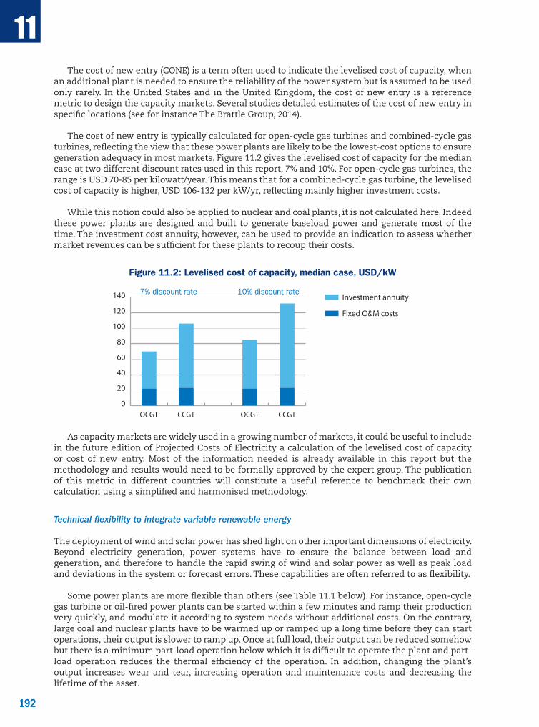
192

11

192

The cost of new entry (CONE) is a term often used to indicate the levelised cost of capacity, when an additional plant is needed to ensure the reliability of the power system but is assumed to be used only rarely. In the United States and in the United Kingdom, the cost of new entry is a reference metric to design the capacity markets. Several studies detailed estimates of the cost of new entry in specific locations (see for instance The Brattle Group, 2014).

The cost of new entry is typically calculated for open-cycle gas turbines and combined-cycle gas turbines, reflecting the view that these power plants are likely to be the lowest-cost options to ensure generation adequacy in most markets. Figure 11.2 gives the levelised cost of capacity for the median case at two different discount rates used in this report, 7% and 10%. For open-cycle gas turbines, the range is USD 70-85 per kilowatt/year. This means that for a combined-cycle gas turbine, the levelised cost of capacity is higher, USD 106-132 per kW/yr, reflecting mainly higher investment costs.

While this notion could also be applied to nuclear and coal plants, it is not calculated here. Indeed these power plants are designed and built to generate baseload power and generate most of the time. The investment cost annuity, however, can be used to provide an indication to assess whether market revenues can be sufficient for these plants to recoup their costs.

Figure 11.2: Levelised cost of capacity, median case, USD/kW

7% discount rate 10% discount rate

0

20

40

60

80

100

120

140

CCGTOCGTCCGTOCGT

Investment annuity

Fixed O&M costs

As capacity markets are widely used in a growing number of markets, it could be useful to include in the future edition of Projected Costs of Electricity a calculation of the levelised cost of capacity or cost of new entry. Most of the information needed is already available in this report but the methodology and results would need to be formally approved by the expert group. The publication of this metric in different countries will constitute a useful reference to benchmark their own calculation using a simplified and harmonised methodology.

Technical flexibility to integrate variable renewable energy

The deployment of wind and solar power has shed light on other important dimensions of electricity. Beyond electricity generation, power systems have to ensure the balance between load and generation, and therefore to handle the rapid swing of wind and solar power as well as peak load and deviations in the system or forecast errors. These capabilities are often referred to as flexibility.

Some power plants are more flexible than others (see Table 11.1 below). For instance, open-cycle gas turbine or oil-fired power plants can be started within a few minutes and ramp their production very quickly, and modulate it according to system needs without additional costs. On the contrary, large coal and nuclear plants have to be warmed up or ramped up a long time before they can start operations, their output is slower to ramp up. Once at full load, their output can be reduced somehow but there is a minimum part-load operation below which it is difficult to operate the plant and part-load operation reduces the thermal efficiency of the operation. In addition, changing the plant’s output increases wear and tear, increasing operation and maintenance costs and decreasing the lifetime of the asset.

193

11

193

Table 11.1: Capability of different power generating technologies to provide flexibility

Start-up timeMaximal change in

30 sec (%)

Maximum ramp rate

(%/min)Open-cycle gas turbine (OCGT) 10-20 min 20-30 20Combined-cycle gas turbine (CCGT) 30-60 min 10-20 5-10Coal plant 1-10 hours 5-10 1-5Nuclear power plant 2 hours – 2 days Up to 5 1-5

Source: NEA, 2012, p. 79.

Needless to say, traditional LCOEs calculated in this report do not capture all these dimensions. When considering an investment decision, however, all these aspects have to be taken into account, in particular in countries with ambitious renewable deployment targets where new conventional power plants will be increasingly used to complement renewables, rather than generate power around the clock.

Modern power plants are designed to be increasingly flexible. It is therefore difficult to separate the different cost components to assess the extra cost of providing flexibility on top of energy. This would require a level of technical expertise beyond what this publication can reasonably achieve.

In addition to generation technologies, other resources can also be utilised in a flexible manner. Demand-response flexibility is a promising emerging solution for medium-size and small consumers. Battery storage can also play an important role if the cost of batteries continues to fall as announced by some manufacturers. All these resources can compete to balance the power system.

Arguably, there is a need to use new metrics to compare the non-energy dimensions of power plant demand-response and storage resources. In a recent publication (IEA, 2014b), an attempt was made to calculate a new metric, the levelised cost of flexibility (LCOF). The results of such calculations for flexibility, however, largely depend on the average capacity factor of the power plant, because in their great majority plants are not built only to provide flexibility, but always primarily to generate power. This interesting notion of LCOF remains complex to manipulate.

Another option to quantify the flexibility dimension of different technologies could be to look at the revenues that each plant earns from different markets, in particular short-term markets for balancing, adjustment and system services. Such an option would be similar to the value factor discussed below but presents the same drawbacks. In many parts of the United States for instance, market monitors assess the breakdown of revenues of typical power plants according to the energy, capacity and ancillary services markets. For a typical gas power plant, ancillary/system services revenues represent typically around USD  10  kW/yr, or 10% of the cost of new entry of such plant. Assuming that ancillary service markets adequately remunerate flexibility, which is a huge simplification, market prices for ancillary services could provide a useful reference in specific instances.

In most cases, however, such revenues are very system-dependent and require having access to detailed market information that is usually not public. Different markets have different installed generation mixes, different definitions for ancillary services and different definitions of flexible products. System operators also have different operating rules. It is therefore difficult to define a harmonised methodology to compare the flexibility of different generation, demand response and storage resources by using market information.

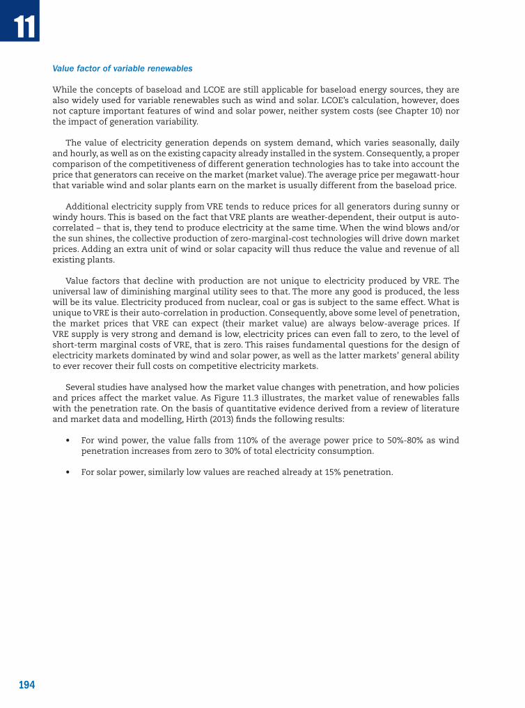
194

11

194

Value factor of variable renewables

While the concepts of baseload and LCOE are still applicable for baseload energy sources, they are also widely used for variable renewables such as wind and solar. LCOE’s calculation, however, does not capture important features of wind and solar power, neither system costs (see Chapter 10) nor the impact of generation variability.

The value of electricity generation depends on system demand, which varies seasonally, daily and hourly, as well as on the existing capacity already installed in the system. Consequently, a proper comparison of the competitiveness of different generation technologies has to take into account the price that generators can receive on the market (market value). The average price per megawatt-hour that variable wind and solar plants earn on the market is usually different from the baseload price.

Additional electricity supply from VRE tends to reduce prices for all generators during sunny or windy hours. This is based on the fact that VRE plants are weather-dependent, their output is auto-correlated – that is, they tend to produce electricity at the same time. When the wind blows and/or the sun shines, the collective production of zero-marginal-cost technologies will drive down market prices. Adding an extra unit of wind or solar capacity will thus reduce the value and revenue of all existing plants.

Value factors that decline with production are not unique to electricity produced by VRE. The universal law of diminishing marginal utility sees to that. The more any good is produced, the less will be its value. Electricity produced from nuclear, coal or gas is subject to the same effect. What is unique to VRE is their auto-correlation in production. Consequently, above some level of penetration, the market prices that VRE can expect (their market value) are always below-average prices. If VRE supply is very strong and demand is low, electricity prices can even fall to zero, to the level of short-term marginal costs of VRE, that is zero. This raises fundamental questions for the design of electricity markets dominated by wind and solar power, as well as the latter markets’ general ability to ever recover their full costs on competitive electricity markets.

Several studies have analysed how the market value changes with penetration, and how policies and prices affect the market value. As Figure 11.3 illustrates, the market value of renewables falls with the penetration rate. On the basis of quantitative evidence derived from a review of literature and market data and modelling, Hirth (2013) finds the following results:

• For wind power, the value falls from 110% of the average power price to 50%-80% as wind penetration increases from zero to 30% of total electricity consumption.

• For solar power, similarly low values are reached already at 15% penetration.

195

11

195

Figure 11.3: Value factor of wind and power

y = -4.8x + 1.2

y = -2.2x + 1.1 0.8

0.9

1

1.1

1.2

1.3

1.4

0% 1% 2% 3% 4% 5% 6% 7% 8% 9% 10%

Vasl

ue fa

ctor

Market share

Solar PV

Wind

0.25

0.50

0.75

1.00

0% 10% 20% 30%

Valu

e fa

ctor

Valu

e fa

ctor

Wind market share

Wind market share

Parameteruncertaintyrange

y = -1.0417x + 0.9669

y = -0.5815x + 0.9465

0

0.2

0.4

0.6

0.8

1

1.2

0% 5% 10% 15% 20% 25% 30% 35% 40% 45%

Dispatch model

Dispatch andinvestment

Source: Updated from Hirth (2013, 2015).

196

11

196

Assessing the value factor of renewables is system-dependent and therefore complex. From a methodological perspective, three approaches can be used: market data, econometrics and structural model of electricity markets.

• Using market data is the simplest solution to calculate the value factor. Electricity market prices exist and are readily available in many markets. Multiplying the hourly output by the hourly price provides an assessment of the value factor of wind and solar power at today’s market conditions. For instance, using market data and plant specific output, Schmalensee (2013) found that output from solar plants was about 32% more valuable on average than output from wind plants. Such a simple calculation provides an indication of current market value, not future ones.

• Econometric analysis can be useful to assess the changes of the value factor for increasing penetration of renewables. Figure 11.3 shows the result of such econometric analysis using historical data for European countries for the period 2007-2012. Hirth found that increasing the market share of wind by one percentage point is estimated to reduce the value factor by 1.62 percentage points in thermal systems. The number of observations, however, is usually very small, which limits the statistical validity of econometric approaches.

• Last, structural models of electricity systems can be used. Structural models are simplified representations of electricity systems that enable to assess different scenarios. Figure 11.3 provides the result of a structural model approach and the range of values under different scenarios. At 30% market share, the value of wind power is reduced to 0.5-0.8 of a constant source. Solar reaches a similar reduction already at 15% penetration.

To sum up, assessing the value factor for different degrees of penetration of wind and solar power is necessary information but remains a complex undertaking. Using econometric modelling or a structural model would not be practical in the context of the EGC series, as one of its main qualities is the comparability of data across a wide range of countries. One possibility would be to look at the current value factor of renewables in different countries by using market prices but this method could not be applied to a forward-looking comparison when countries wish to increase their share of VREs.

11.6 Conclusions

In the coming years, the NEA/IEA series on the Projected Costs of Generating Electricity faces a challenge to its ability to provide cost information that is both useful and relevant. It will need to adapt in order to reflect changes in the structure and economics of electricity markets in OECD countries. The most important of these changes is the large-scale introduction of variable renewables (VRE) such as wind and solar. In particular, the well-worn metric of LCOE will need to be complemented by additional metrics as the notion of baseload power provision risks losing some of its relevance, and other services to the electricity system, such as capacity or flexibility provision are growing in importance. This is, of course, not a challenge that is unique to the Projected Costs report but a general consequence of the fact that the headlong rush into the subsidisation of VRE has landed the electricity sectors of OECD countries in largely unchartered territory.

In order to kick-start the discussion with member countries, as well as with the community of electricity experts at large, the IEA and NEA Secretariats have thus proposed a series of four metrics that would be complementary to the traditional LCOE measures. These four metrics currently consist of:

• the capacity credit measuring a technology’s per unit of installed capacity contribution to system adequacy;

• the cost of new entry for providing an additional unit of capacity;

• a flexibility metric assessing the ability to ride out changes in supply and demand;

• a value factor of VRE as a function of their market share.

197

11

197

The pertinence and feasibility of these metrics over a wide array of countries and technologies will need to be discussed in the coming years, before work on a ninth edition can begin. Defining framework conditions and reference scenarios will be a necessary part of this task. While this will put a considerable additional burden on member countries’ experts and the IEA and NEA Secretariats, this work will also constitute a fascinating intellectual and institutional challenge. If mastered, the results would allow discussions over policy making in OECD power markets to continue for many years to come and would also allow the Projected Costs studies to remain an indispensable reference for policy makers, modellers and electricity market experts.

References

IEA (2014a), World Energy Outlook, OECD, Paris.

IEA (2014b), Energy Technology Perspectives, OECD, Paris.

IEA (2014c), The Power of Transformation. Wind, Sun and the Economics of Flexible Power Systems, OECD, Paris.

Hirth, L. (2013), “The market value of variable renewables: The effect of solar and wind power variability on their relative price”, Energy Economics, Vol. 38, pp. 218-236.

Hirth, L. (2015): “The market value of solar power: Is photovoltaics cost-competitive?”, IET Renewable Power Generation, Vol. 9(1), pp. 37-45.

NEA (2012), Nuclear Energy and Renewables: System Effects in Low-carbon Electricity Systems, OECD, Paris.

NEA (2015), Nuclear New Build: Insights into Financing and Project Management, OECD, Paris.

Schmalensee (2013), “The Performance of US Wind and Solar Generating Plants”, MIT CEEPR working paper, http://web.mit.edu/ceepr/www/publications/workingpapers/2013-012.pdf.

The Brattle Group (2014), Cost of New Entry Estimates for Combustion Turbine and Combined-Cycle Plants in PJM, The Brattle Group, www.brattle.com/system/publications/pdfs/000/005/010/original/Cost_of_New_Entry_Estimates_for_Combustion_Turbine_and_Combined_Cycle_Plants_in_PJM.pdf?1400252453.

Annexes

201

A1

201

Annex

The EGC spreadsheet model for calculating LCOE

The actual calculations of the levelised cost of electricity (LCOE) for all countries were undertaken with the help of a simple spreadsheet model according to a set of common basic assumptions. Its key purpose was to generate LCOE data in a transparent and easily reproducible manner. The electricity generating costs (EGC) spreadsheet model is intended to be a flexible, transparent structure able to accommodate different assumptions without losing the underlying coherence of the exercise of comparing national cost figures for power generation over different technologies.

Only a few parameters can be included in any model that works for 181 plants from 22 different sources (19 OECD member countries and 3 non-member countries). In practice, many parameters not included in the model may have significant influence on actual electricity generating costs. First and foremost, government policies ranging from market design and competition rules to loan guarantees and implicit or explicit subsidies and taxes, have not been included in the calculations. One may consider this a shortcoming of this report. In reality, any inclusion of parameters beyond raw, technical costs would have rendered any such comparative study over more than a few countries meaningless. This does not indicate that more in-depth research on the basis of a broader set of factors affecting generating costs in individual cases could not yield useful and interesting results.

The EGC spreadsheet model is contained in many Excel worksheets. It is based on a similar, simpler model used in preceding versions of the EGC report since 1981. The EGC spreadsheet model has been significantly modified in its form, if not in its function, in order to continue to improve readability and transparency of all operations. In particular: default assumptions and inputs based on the questionnaire responses have been moved into separate worksheets; a “data used” worksheet has been added that shows on one page the exact combination of default and user input assumptions being used by the model; and a summary page has been added that shows all results for all modelled technologies at the various discount rates and capacity factors. In addition, the model now automatically generates many of the charts presented in later chapters.

In the following sections, the different elements of the model and its workings are briefly presented. For all quantitative assumptions, see Chapter  2 “Methodology, conventions and key assumptions”.

1. Default data

The default data worksheet sets the basic assumptions used for all technologies modelled. This includes generic assumptions that apply to all (relevant) technologies, technical assumptions, assumptions related to construction and decommissioning, fuel cost assumptions, and exchange rates.

Generic assumptions include the carbon price, heat price, the commissioning date (1 January 2020) and a default discount rate. Technical assumptions include technology-specific default assumptions: electrical efficiency (if relevant); lifetime; capacity factor (for electricity and, in the case of CHP,

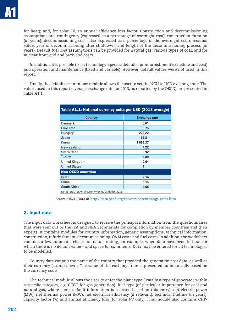
202

A1

202

for heat); and, for solar PV, an annual efficiency loss factor. Construction and decommissioning assumptions are: contingency (expressed as a percentage of overnight cost); construction duration (in years); decommissioning cost (also expressed as a percentage of the overnight cost); residual value; year of decommissioning after shutdown; and length of the decommissioning process (in years). Default fuel cost assumptions can be provided for natural gas, various types of coal, and for nuclear front-end and back-end costs.

In addition, it is possible to set technology-specific defaults for refurbishment (schedule and cost) and operation and maintenance (fixed and variable). However, default values were not used in this report.

Finally, the default assumptions module allows the user to set the NCU to USD exchange rate. The values used in this report (average exchange rate for 2013, as reported by the OECD) are presented in Table A1.1.

Table A1.1: National currency units per USD (2013 average)

Country Exchange rate

Denmark 5.61Euro area 0.75Hungary 222.22Japan 96.8Korea 1 095.37New Zealand 1.22Switzerland 0.92Turkey 1.89United Kingdom 0.64United States 1

Non-OECD countries

Brazil 2.14China 6.15South Africa 9.66Note: Total, national currency units/US dollar, 2013.

Source: OECD Data at http://data.oecd.org/conversion/exchange-rates.htm

2. Input data

The input data worksheet is designed to receive the principal information from the questionnaires that were sent out by the IEA and NEA Secretariats for completion by member countries and their experts. It contains modules for country information, generic assumptions, technical information, construction, refurbishment, decommissioning, O&M costs and fuel costs. In addition, the worksheet contains a few automatic checks on data – noting, for example, when data have been left out for which there is no default value – and space for comments. Data may be entered for all technologies to be modelled.

Country data contain the name of the country that provided the generation cost data, as well as their currency (a drop-down). The value of the exchange rate is presented automatically based on the currency code.

The technical module allows the user to enter the plant type (usually a type of generator within a specific category, e.g. CCGT for gas generation), fuel type (of particular importance for coal and natural gas, where some default information is selected based on this entry), net electric power (MW), net thermal power (MW), net electrical efficiency (if relevant), technical lifetime (in years), capacity factor (%) and annual efficiency loss (for solar PV only). This module also contains CHP-

203

A1

203

specific inputs, namely annual heat production (in GWh, for CHP), net thermal capacity (MWth, for CHP), electrical efficiency (condensing), capacity factor for electrical efficiency condensing, and capacity factor for heat.

The construction module allows the user to set a different commissioning date (though this is ignored in modelling), total overnight cost (with sub-fields for preconstruction and owners cost, used for information purposes only), contingency cost, construction duration, and expense schedule (in terms of percentage per year; this must add up to 100%).

The refurbishment module allows the user to set a refurbishment schedule for the plant, up to a maximum of three refurbishments over its technical lifetime. For each refurbishment, the user must provide the year and the overnight cost (NCU/kWe).

The decommissioning module allows the user to override the default decommissioning costs, residual value, year of decommissioning (in terms of number of years after shutdown) and length of decommissioning (in years).

The O&M module allows the user to enter the fixed (NCU per MW) and variable (NCU per MWh) O&M costs.

Finally, the fuel cost module allows the user to enter specific fuel-related costs for relevant technologies. For nuclear, this includes front-end costs and back-end, or waste management, costs. For coal, this includes the cost (in NCU per tonne, NCU per GJ or NCU per MWh), the calorific value of the fuel, and either the average CO2 emissions factor or the IPCC factor. For natural gas, this includes the fuel cost (in NCU per MMBtu, per GJ, or per MWh), as well as the calorific value and the CO2 emissions factor or IPCC factor. The same fuel information can also be entered for CHP plants.

3. Data used

The data used worksheet is identical in structure to the input data worksheet. However, it does not allow for any inputs. Instead, it draws from the input data worksheet when data are present, and from the default data worksheet when the relevant input data cell is blank. Default data, when used, are presented in green, while input data are presented in black. The various levelised cost calculators draw their inputs from the data used worksheet.

4. Levelised cost calculator(s)

The EGC spreadsheet model contains one levelised cost calculator worksheet for each technology modelled. This worksheet will be most familiar to users of the previous EGC spreadsheet modules, as it contains the same core functionality. The major difference is that the work of setting the input values is now done separately.

The levelised cost calculator contains eight modules separated into two parts (A and B), and a part C containing two discount schedules – one in NCU terms and one in USD terms. The three parts and various modules are described below.

Part A

Part A of the ECG Spreadsheet Model contains five basic modules (identification, basic assumptions, questionnaire information, generating costs and lifetime generating costs) that provide all necessary information for readers only interested in the input and output data but not in the working of the model and its underlying assumptions.

204

A1

204

1. Identification

Module 1 provides the information that associates a given set of data with a specific country, fuel category, technology and technology type (if applicable). It also specifies in which NCU the data are provided.

2. Basic assumptions

This module lists the plant’s net capacity, net electrical efficiency (if relevant), capacity factor, lifetime, default discount rate, carbon price, commission date, and exchange rate (NCU/USD). Certain technology-specific assumptions may also be listed, such as price of uranium (for nuclear), heat price (for CHP), and annual efficiency loss (for solar PV). Capacity is plant-specific, though it does not impact the final LCOE results. For nuclear, coal and CCGTs, plant-specific capacity factors are used if provided, but in addition the results are calculated at assumed capacity factors of 85% and 50%. For renewables and other technologies, plant-specific capacity factors provided by countries are always used.

3. Questionnaire information

Module 3 presents the principal information from the questionnaire responses. It contains entries for the costs of pre-construction, construction, contingency, refurbishment, decommissioning, fixed and variable operations and maintenance, fuel, carbon, and waste management costs. A separate, related module shows the construction profile, allowing for a maximum of eight years of construction time.

4. Generating costs

Module 4 contains the results of the ECG Spreadsheet Model in terms of LCOE per MWh of electricity. The results are reported separately for the individual cost items as well as for a) total capital costs, b) total variable costs, and c) total generating costs, the key figure of merit for this report. The results are derived by feeding the values of modules 2 and 3 into the fuel, carbon and CHP modules of Part B and into the discounting schedules I (NCU) and II (USD) of Part C.

The results are reported once in NCU and again in USD, to verify the consistency of the different elements. The first set of results reported in USD is attained by converting the NCU results, obtained through bottom-up calculations on the basis of discounting schedule I (NCU). The second set of results reported in USD is obtained through bottom-up calculations on the basis of discounting schedule II (USD). When the two figures are consistent, there is high probability that the model is working correctly.

In addition to module 4, the EGC Spreadsheet Model contains one or three related modules, depending on the technology: module 4a (all technologies), and modules 4b and 4c (only for natural gas, nuclear and coal).

Module 4a contains the sensitivity analysis for the discount rate, presenting the results of additional levelised cost calculations for discount rates of 3%, 5%, 7%, 10% and 12%. Module 4b contains sensitivity results at all of these discount rates under an assumed capacity factor of 85% – overriding the user-provided capacity factor, if it differs. Finally, module 4c provides the sensitivity results for each discount rate under an assumed capacity factor of 50%.

5. Lifetime generating costs

Module 5 reports total discounted generating cost and the LCOE in a synthetic manner.

205

A1

205

Part B

Part B contains the fossil fuel module (module 6), the CO2 or carbon module (module 7), and the CHP module for calculating heat credits (module 8). In principle, these modules work autonomously on the basis of the information provided in module 2, which is then transformed on the basis of generic technical assumptions, such as carbon content or conversion efficiencies. Where available, the generic technical assumptions were substituted with country-specific national assumptions.

6. Fossil fuel module

This module calculates fuel costs per MWh on the basis of price information for coal in USD per tonne and for natural gas in USD per MMBtu. Prices for coal are converted into prices per GJ. To this aim, where harmonised fuel prices have been used for traded hard coal in importing countries, it has been assumed that a tonne of hard coal corresponds to 25 GJ of energy per tonne (see the latest IEA statistical information available).

In the case of lignite, which is domestically produced and consumed, and is quite heterogeneous, national information for prices and heat content were used. Fuel costs for coal and natural gas are subsequently adjusted by the electrical conversion efficiency of each technology.

7. CO2 module

The CO2 module calculates the carbon cost per MWh. Whenever available, national data on carbon emissions per MWh were used. Otherwise data were derived from the report by the Intergovernmental Panel on Climate Change (IPCC 2006, Chapter 2 “Stationary Combustion”, p. 2.16). Typically, carbon emissions are around 100 tCO2/terajoules for hard coal and 50 tCO2/terajoules for natural gas. With standard electric conversion factors of 40% and 55%, this amounts to emissions of 0.9 tCO2/MWh for electricity from hard coal and of 0.33 tCO2/MWh for electricity from CCGTs.

In the case of CHP plants, all carbon emissions were allocated to electricity production. This seems to produce counter-intuitive results because carbon emissions per MWh are thus higher than at electricity-only plants. However, in the cost calculations, this effect vanishes, because a heat credit is applied to the unit costs of the CHPs. Including total CO2 emissions for CHP to electricity output not only raises carbon costs, but it also raises the credit for heat output (because no carbon costs apply to the heat). The final result reflects the economic cost advantages of CHP and is consistent with the LCOE methodology.

8. CHP module for calculating the heat credit

The CHP module for calculating the heat credit continues an accounting convention used in earlier EGC reports. Given that CHP produces heat as well as power, one cannot impute the total generating costs to power alone. Parcelling out cost shares, however, is highly impractical because heat and power are genuine joint products. The convention adopted is to impute to power generation the total costs of generation minus the value of the heat produced.

To arrive at a CHP heat credit per MWh of electricity, one must establish first the total value of the heat produced over the lifetime of the plant by multiplying total heat output by its per-unit value. The total value of the heat output is then divided by the lifetime electricity production to obtain the per-MWh heat credit.

206

A1

206

Part C

9. Discounting schedule I (NCU) and II (USD) with variable cost sub-model

Part C contains the two discounting schedules that extend from 2012 to 2119 (though calculations are only performed for years corresponding to the lifetime of the plant – that is, years of construction, years of operation, and years of decommissioning and dismantling). Discounting schedule I is in terms of NCU and discounting schedule II in terms of USD. Both have been arranged to allow maximum transparency in terms of inter-temporal costs (vertically) and in terms of the different cost components (horizontally). Its structure is determined by the modellers according to the methodological conventions adopted for calculating LCOE with the EGC spreadsheet model.

207

A2

207

Annex

List of abbreviations and acronyms

AC alternating current

ALWR advanced light water reactor

A-USC advanced ultra-supercritical

BICGT biomass internal combustion gas turbine

BIGCC biomass internal gasification combined-cycle

BOS balance of system

BWR boiling water reactor

CAES compressed air energy storage

CAPEX capital expenditure

CCGT combined-cycle gas turbine

CCS carbon capture and storage (or sequestration)

CFDs contracts for differences

CHP combined heat and power

CPV concentrating photovoltaic

c-Si crystalline silicon

CSP concentrating solar power

DC direct current

D&D decommissioning and dismantlement

DNI direct normal irradiance

EGC electricity generating costs

EGS enhanced geothermal systems

EOR enhanced oil recovery

ETP IEA Energy Technology Perspectives study

ETS emissions trading scheme

FCs fuel cells

FiTs feed-in-tariffs

Gen IV generation IV

GJ gigajoules

HLW high-level waste

208

A2

208

HTR high-temperature reactor

IDC interest during construction

IGCC integrated gasification combined-cycle

IPCC Intergovernmental Panel on Climate Change

kWe kilowatt of electricity capacity

LCOE levelised cost of electricity

LFR lead-cooled fast reactor

LHV lower heating value

LNG liquefied natural gas

LWR light water reactor

MMBtu million British thermal units

MWh megawatt-hour

NCU national currency unit

NGCC natural gas combined-cycle

OCGT open-cycle gas turbine

O&M operation and maintenance

ORC Overnight refurbishment cost

PV photovoltaic

PWR pressurised water reactor

RD&D research, development and demonstration

SC supercritical

SFR sodium-cooled fast reactor

SMR small modular reactor

SOFC solid oxide fuel cell

USD US dollars

VRE variable renewable energy

2DS 2-degree scenario

2DS hi-Ren high-renewable variant

209

List of participating members of the EGC Expert Group

Data for this report was provided through the expert group, except in the case of China, in which case the IEA and NEA Secretariats collected publicly available data from a variety of Chinese sources. The IEA and NEA Secretariats are happy to refer any enquiries about data to the respective experts. Please contact for this purpose Matthew Wittenstein (matthew.wittenstein@iea.org) or Geoffrey Rothwell (geoffrey.rothwell@oecd.org).

Country representatives

Michael Sorger Energy-Control GmbH (Austria)

Kenneth Bruninx KU Leuven Energy Institute (Belgium)

William D’haeseleer (Chair) KU Leuven Energy Institute (Belgium)

Erik Delarue KU Leuven Energy Institute (Belgium)

Kenneth Van Den Bergh KU Leuven Energy Institute (Belgium)

Rikke Naeraa Danish Ministry of Climate, Energy and Building (Denmark)

Esa Vakkilainen Lappeenranta University of Technology (Finland)

Pierre Boutot Direction Générale de l’Énergie et du Climat (France)

Antoine Caron Direction Générale de l’Énergie et du Climat (France)

Thierry Duquesnoy Commissariat à l’énergie atomique et aux énergies alternatives, Saclay (France)

Matthias Löhrl Bundesministerium für Wirtschaft und Energie (Germany)

Maike Schmidt Zentrum für Sonnenenergie und Wasserstoff Forschung (ZSW) (Germany)

Alfred Voβ University Stuttgart, IER (Germany)

Attila Hugyecz Department for Nuclear Energy Analysis (Hungary)

Bálint Virág MVM Paks II. Zrt. (Hungary)

Luca Benedetti Gestore dei Servizi Energetici (Italy)

Luca Miraglia Gestore dei Servizi Energetici (Italy)

Marco Rao ENEA (Italy)

Yuji Matsuo (Co-chair) The Institute of Energy Economics (Japan)

Tomoko Murakami The Institute of Energy Economics (Japan)

Kazushige Tanaka Permanent Delegation of Japan to the OECD (Japan)

210

Sung Jin Cho Korean Energy Economics Institute (Korea)

Byeoung Kug Lee Korea Hydro and Nuclear Power Co. (Korea)

Chan Kook Park Korean Energy Economics Institute (Korea)

Ho Hyern Youn Korea Power Exchange (Korea)

Ozge Özdemir Energy Research Centre of the Netherlands (Netherlands)

Olgierd Skonieczny PGE Polska Gruipa Energetyczna SA (Poland)

Luisa Basilio Directorate General for Energy and Geology (Portugal)

Jeronimo Cunha Directorate General for Energy and Geology (Portugal)

Maria Sicilia Salvadores Enagás, S.A. (Spain)

Stephen Baker Department of Energy and Climate Change (United Kingdom)

David Meads Department of Energy and Climate Change (United Kingdom)

Maria Tamba Department of Energy and Climate Change (United Kingdom)

Birgit Wosnitza Department of Energy and Climate Change (United Kingdom)

Douglas J. Arent National Renewable Energy Laboratory (United States)

Matthew P. Crozat Department of Energy (United States)

Francesco Ganda Argonne National Laboratory (United States)

Ed Hoffman Argonne National Laboratory (United States)

Ookie Ma Department of Energy (United States)

Industry representatives

Emeric Jannet AREVA

John Paffenbarger Exelon Corporation

Rémy Ferrato Électricité de France

Christophe Trzpit Électricité de France

Christian Stolzenberger Eurelectric/VGB Powertech

Oliver Then Eurelectric/VGB Powertech

Representatives of international organisations

David Shropshire IAEA

Marc Deffrennes EC (at the NEA since October 2014)

Manuel Baritaud IEA

Paolo Frankl IEA

Michael Waldron IEA

Keisuke Sadamori IEA

Laszlo Varro IEA

Matthew Wittenstein IEA

Ron Cameron NEA (until July 2014)

Marco Cometto NEA

211

Jan Horst Keppler NEA

Geoffrey Rothwell NEA

Further contributors

Others have contributed to the report with data, advice or help on questions of methodology:

Marco Baroni IEA

Emanuele Bianco IEA

Gina Downes Eskom Holdings (South Africa)

Manuela Fonseca Directorate General for Energy and Geology (Portugal)

Simon Green Department of Energy and Climate Change (United Kingdom)

Michael Hackethal Bundesministerium für Wirtschaft und Technologie (Germany)

Gilberto Hollauer Ministry of Mines and Energy (Brazil)

Joon Han Kim Korea Power Exchange (Korea)

Steve Lennon Eskom Holdings (South Africa)

Roger Lundmark Swissnuclear (Switzerland)

Luis H. A. Mijares Ministry of Industry, Energy and Tourism (Spain)

Simon Mueller IEA

Henri Paillère NEA

Cédric Philibert IEA

Harald Proidl Energy-Control GmbH (Austria)

Noor Miza Muhamad Razali Consultant for IEA

Cecilia Tam IEA

Alexandre Tavin Direction Générale du Trésor (France)

Davina Till IEA

Cyndia Yu Consultant for NEA (summer 2014)

OECD PUBLICATIONS, 2 rue André-Pascal, 75775 Paris Cedex 16, France.

Photo credits pages 21, 109 and 135: Solar panels (NEA), Brokdorf nuclear power plant, Germany (Alois Staudacher), coal power station and cement plant at night (Cozyta, Shutterstock) and

industria wind installations (Carlos Castilla, Shutterstock).

Projected Costs of Generating Electricity

This joint report by the International Energy Agency (IEA) and the Nuclear Energy Agency (NEA) is the eighth in a series of studies on electricity generating costs. As policy makers work to ensure that the power supply is reliable, secure and affordable, while making it increasingly clean and sustainable in the context of the debate on climate change, it is becoming more crucial that they understand what determines the relative cost of electricity generation using fossil fuel, nuclear or renewable sources of energy. A wide range of fuels and technologies are presented in the report, including natural gas, coal, nuclear, hydro, solar, onshore and offshore wind, biomass and biogas, geothermal, and combined heat and power, drawing on a database from surveys of investment and operating costs that include a larger number of countries than previous editions.

The analysis of more than 180 plants, based on data covering 22 countries, reveals several key trends, pointing, for example, to a significant decline in recent years in the cost of renewable ge-neration. The report also reveals that nuclear energy costs remain in line with the cost of other baseload technologies, particularly in markets that value decarbonisation. Overall, cost drivers of the different generating technologies remain both market-specific and technology-specific.

Readers will find a wealth of details and analysis, supported by over 200 figures and tables, underlining this report’s value as a tool for decision makers and researchers concerned with energy policies, climate change and the evolution of power sectors around the world.

Projected C

osts of Gen

erating Electricity – 2015 Ed

ition

Nuclear Energy Agency (NEA)12 boulevard des Îles92130 Issy-les-Moulineaux, FranceTel.: +33 (0)1 45 24 10 15nea@oecd-nea.org www.oecd-nea.org

International Energy Agency (IEA)9 rue de la Fédération

75739 Paris Cedex 15, FranceTel.: +33 (0)1 40 57 65 00

info@iea.org www.iea.orgNEA No. 7057