Generalized Correspondence-LDA Models (GC-LDA)for Identifying Functional Regions in the Brain

Timothy N. RubinIndiana University

timrubin@indiana.edu

Oluwasanmi KoyejoUniversity of Illinois at Urbana-Champaign

sanmi@illinois.edu

Michael N. JonesIndiana University

jonesmn@indiana.edu

Tal YarkoniUniversity of Texas at Austintyarkoni@utexas.edu

Abstract

This paper presents Generalized Correspondence-LDA (GC-LDA), a generalizationof the Correspondence-LDA model that allows for variable spatial representationsto be associated with topics, and increased flexibility in terms of the strengthof the correspondence between data types induced by the model. We presentthree variants of GC-LDA, each of which associates topics with a different spatialrepresentation, and apply them to a corpus of neuroimaging data. In the context ofthis dataset, each topic corresponds to a functional brain region, where the region’sspatial extent is captured by a probability distribution over neural activity, and theregion’s cognitive function is captured by a probability distribution over linguisticterms. We illustrate the qualitative improvements offered by GC-LDA in termsof the types of topics extracted with alternative spatial representations, as wellas the model’s ability to incorporate a-priori knowledge from the neuroimagingliterature. We furthermore demonstrate that the novel features of GC-LDA improvepredictions for missing data.

1 Introduction

A primary goal of cognitive neuroscience it to find a mapping from neural activity onto cognitiveprocesses–that is, to identify functional networks in the brain and the role they play in supportingmacroscopic functions. A major milestone towards this goal would be the creation of a “functional-anatomical atlas” of human cognition, where, for each putative cognitive function, one could identifythe regions and brain networks within the region that support the function.

Efforts to create such functional brain atlases are increasingly common in recent years. Most studieshave proceeded by applying dimensionality reduction or source decomposition methods such asIndependent Component Analysis (ICA) [4] and clustering analysis [9] to large fMRI datasets suchas the Human Connectome Project [10] or the meta-analytic BrainMap database [8]. While suchwork has provided valuable insights, these approaches also have significant drawbacks. In particular,they typically do not jointly estimate regions along with their mapping onto cognitive processes.Instead, they first extract a set of neural regions (e.g., via ICA performed on resting-state data), andthen in a separate stage—if at all—estimate a mapping onto cognitive functions. Such approaches donot allow information regarding cognitive function to constrain the spatial characterization of theregions. Moreover, many data-driven parcellation approaches involve a hard assignment of each brainvoxel to a single parcel or cluster, an assumption that violates the many-to-many nature of functionalbrain networks. Ideally, a functional-anatomical atlas of human cognition should allow the spatial

29th Conference on Neural Information Processing Systems (NIPS 2016), Barcelona, Spain.

and functional correlates of each atom or unit to be jointly characterized, where the function of eachregion constrains its spatial boundaries, and vice-versa.

In the current work, we propose Generalized Correspondence LDA (GC-LDA) – a novel generaliza-tion of the Correspondence-LDA model [3] for modeling multiple data types, where one data typedescribes the other. While the proposed approach is general and can be applied to a variety of data,our work is motivated by its application to neuroimaging meta-analysis. To that end, we considerseveral GC-LDA models that we apply to the Neurosynth [12] corpus, consisting of text and neuralactivation data from a large body of neuroimaging publications. In this context, the models extract aset of neural “topics”, where each topic corresponds to a functional brain region. For each topic, themodel provides a description of its spatial extent (captured via probability distributions over neuralactivation) and cognitive function (captured via probability distributions over linguistic terms). Thesemodels provide a novel approach for jointly identifying the spatial location and cognitive mapping offunctional brain regions, that is consistent with the many-to-many nature of functional brain networks.Furthermore, to the best of our knowledge, one of the GC-LDA variants provides the first automatedmeasure of the lateralization of cognitive functions, based on large-scale imaging data.

The GC-LDA and Correspondence-LDA models are extensions of Latent Dirichlet Allocation (LDA)[3]. Several Bayesian methods with similarities (or equivalences) to LDA have been applied todifferent types of neuroimaging data. Poldrack et al. (2012) used standard LDA to derive topicsfrom the text of the Neurosynth database and then projected the topics onto activation space based ondocument-topic loadings [7]. Yeo et al. (2014) used a variant of the Author-Topic model to model theBrainMap Database [13]. Manning et al. (2014) described a Bayesian method “Topographic FactorAnalysis” to identify brain regions based on the raw fMRI images (but not text) extracted from a setof controlled experiments, which can later be mapped on functional categories [5].

Relative to the Correspondence-LDA model, the GC-LDA model incorporates: (i) the ability toassociate different types of spatial distributions with each topic, (ii) flexibility in how strictly themodel enforces a correspondence between the textual and spatial data within each document, and (iii)the ability to incorporate a-priori spatial structure, e.g., encouraging relatively homologous functionalregions located in each brain hemisphere. As we show, these aspects of GC-LDA have a significanteffect on the quality of the estimated topics, as well as on the models’ ability to predict missing data.

2 Models

In this paper we propose a set of unsupervised generative models based on the Correspondence-LDAmodel [2] that we use to jointly model text and brain activations from the Neurosynth meta-analyticdatabase [12]. Each of these models, as well as Correspondence-LDA, can be viewed as special casesof a broader model that we will refer to as Generalized Correspondence-LDA (GC-LDA). In thesection below, we describe the GC-LDA model and its relationship to Correspondence-LDA. Wethen detail the specific instances of the model that we use throughout the remainder of the paper. Asummary of the notation used throughout the paper is provided in Table 1.

2.1 Generalized Correspondence LDA (GC-LDA)

Each document d in the corpus is comprised of two types of data: a set of word tokens{w

(d)1 , w

(d)2 , ..., w

(d)

N(d)w

}consisting of unigrams and/or n-grams, and a set of peak activation tokens{

x(d)1 , x

(d)2 , ..., x

(d)

N(d)x

}, where N (d)

w and N (d)x are the number of words and peak tokens in document

d, respectively. In the target application, each token xi is a 3-dimensional vector corresponding tothe peak activation coordinates of a value reported in fMRI publications. However, we note thatthis model can be directly applied to other types of data, such as segmented images, where each xicorresponds to a vector of real-valued features extracted from each image segment (c.f. [2]).

GC-LDA is described by the following generative process (depicted in Figure 1 (A)):

1. For each topic t ∈{

1, ..., T}1:

1To make the model fully generative, one could additionally put a prior on the spatial distribution parametersΛ(t) and sample them. For the purposes of the present paper we do not specify a prior on these parameters, andtherefore leave this out of the generative process.

2

Table 1: Table of notation used throughout the paper

Model specificationNotation Meaningwi, xi The ith word token and peak activation token in the corpus, respectively

N(d)w , N (d)

x The number of word tokens and peak activation tokens in document d, respectivelyD The number of documents in the corpusT The number of topics in the modelR The number of components/subregions in each topic’s spatial distribution (subregions model)zi Indicator variable assigning word tokens to topicsyi Indicator variable assigning activation tokens to topics

z(d), y(d) The set of all indicator variables for word tokens and activation tokens in document dNY Dtd The number of activation tokens within document d that are assigned to topic tci Indicator variable assigning activation tokens to subregions (subregion models)

Λ(t) Placeholder for all spatial parameters for topic tµ(t), σ(t) Gaussian parameters for topic tµ(t)r , σ(t)

r Gaussian parameters for subregion r in topic t (subregion models)φ(t) Multinomial distribution over word types for topic tφ(t)w Probability of word type w given topic tθ(d) Multinomial distribution over topics for document dθ(d)t Probability of topic t given document dπ(t) Multinomial distribution over subregions for topic t (subregion models)π(t)r Probability of subregion r given topic t (subregion models)

β, α, γ Model hyperparametersδ Model hyperparameter (subregion models)

(a) Sample a Multinomial distribution over word types φ(t) ∼ Dirichlet(β)

2. For each document d ∈ {1, ..., D}:

(a) Sample a Multinomial distribution over topics θ(d) ∼ Dirichlet(α)

(b) For each peak activation token xi, i ∈{

1, ..., N(d)x

}:

i. Sample indicator variable yi from Multinomial(θ(d))ii. Sample a peak activation token xi from the spatial distribution: xi ∼ f(Λ(yi))

(c) For each word token wi, i ∈{

1, ..., N(d)W

}:

i. Sample indicator variable zi from Multinomial(

NY D1d +γ

N(d)x +γ∗T

,NY D

2d +γ

N(d)x +γ∗T

, ...,NY D

Td +γ

N(d)x +γ∗T

),

where NY Dtd is the number of activation tokens y in document d that are assigned to topic t,

N(d)x is the total number of activation tokens in d, and γ is a hyperparameter

ii. Sample a word token wi from Multinomial(φ(zi))

Intuitively, in the present application of GC-LDA, each of the topics corresponds to a functional regionof the brain, where the linguistic features for the topic describe the cognitive processes associatedwith the spatial distribution of the topic. The resulting joint distribution of all observed peak activationtokens, word tokens, and latent parameters for each individual document in the GC-LDA model is asfollows:

p(x,w, z, y, θ) = p(θ|α)·

N(d)x∏

i=1

p(yi|θ(d))p(xi|Λ(yi))

·N(d)

w∏j=1

p(zj |y(d), γ)p(wj |φ(zj))

(1)

Note that when γ = 0, and the spatial distribution for each topic is specified as a single multivariateGaussian distribution, the model becomes equivalent to a smoothed version of the CorrespondenceLDA model described by Blei & Jordan (2003) [2].2

2We note that [2] uses a different generative description for how the zi variables are sampled conditionalon the y(d)i indicator variables; in [2], zi is sampled uniformly from (1, ..., N (d)

y ), and then wi is sampled fromthe multinomial distribution of the topic y(d)i that zi points to. This ends up being functionally equivalent to

3

T R

D NW

γ

w

NX

y

x

θ α

T φβ µ σ

z

D NW

γ

w

NX

y

x

θ α

φβ µ σ

z

π

c

δ

D NW

γ

w

NX

y

x

θ α

T φβ λ1 λN…

z

(A) (B) (C)

Figure 1: (A) Graphical model for the Generalized Correspondence-LDA model, GC-LDA. (B)Graphical model for GC-LDA with spatial distributions modeled as a single multivariate Gaussian(equivalent to a smoothed version of Correspondence-LDA if γ = 0)2. (C) Graphical model forGC-LDA with subregions, with spatial distributions modeled as a mixture of multivariate Gaussians

A key aspect of this model is that it induces a correspondence between the number of activationtokens and the number of word tokens within a document that will be assigned the same topic. Thehyperparameter γ controls the strength of this correspondence. If γ = 0, then there is zero probabilitythat a word for document d will be sampled from topic t if no peak activations within d were sampledfrom t. As γ becomes larger, this constraint is relaxed, and it becomes more likely for a documentto sample a word from a topic from which it sampled no peak activations. Although intuitively onemight want γ to be zero in order to maximize the correspondence between the spatial and linguisticinformation, we have found that in practice, using a non-zero γ leads to significantly better modelperformance. We conjecture that using a non-zero γ allows the parameter space to be more efficientlyexplored during inference, since it allows peaks to be assigned to topics to which no words wereassigned, and vice versa. It is also likely that a non-zero γ improves the model’s ability to handle datasparsity and noise in high dimensional spaces, in the same way that the α and β hyperparametersserve this role in standard LDA [1].

2.2 Versions of GC-LDA Employed in Current Paper

There are multiple reasonable choices for the spatial distribution p(xi|Λ(yi)) in GC-LDA, dependingupon the application and the goals of the modeler. For the purposes of the current paper, we consideredthree variants that are motivated by the target application. The first model shown in Figure 1.Bemploys a single multivariate Gaussian distribution for each topic’s spatial distribution – and istherefore equivalent to a smoothed version of Correspondence-LDA if setting γ = 0. The generativeprocess for this model is the same as specified above, with generative step (b.ii) modified as follows:Sample peak activation token xi from from a Gaussian distribution with parameters µ(yi) and σ(yi).We refer to this model as the “no-subregions” model.

The second model and third model both employ Gaussian mixtures with R = 2 components foreach topic’s spatial distribution, and are shown in Figure 1.C. Employing a Gaussian mixture givesthe model more flexibility in terms of the types of spatial distributions that can be associated witha topic. This is notably useful in modeling spatial distributions associated with neural activity, asit allows the model to learn topics where a single cognitive function (captured by the linguisticdistribution) is associated with spatially discontiguous patterns of activations. In the second GC-LDAmodel we present—which we refer to as the “unconstrained subregions” model—the Gaussianmixture components are unconstrained. In the third version of GC-LDA—which we refer to asthe “constrained subregions” model—the components are constrained based on findings from theneuroimaging literature. Specifically, the Gaussian components are constrained to have symmetricmeans with respect to their distance from the origin along the horizontal spatial axis (a plane

the generative description for zi given here when γ = 0. Additionally, in [2], no prior is put on φ(t), unlike inGC-LDA. Therefore, when using GC-LDA with a single multivariate Gaussian and γ = 0, it is equivalent to asmoothed version of Correspondence-LDA. Dirichlet priors have been demonstrated to be beneficial to modelperformance [1], so including a prior on φ(t) in GC-LDA should have a positive impact.

4

corresponding to the longitudinal fissure in the brain). This constraint is consistent with results frommeta-analyses of the fMRI literature, where most studied functions display a high degree of bilateralsymmetry [e.g., 6, 12].

The use of mixture models for representing the spatial distribution in GC-LDA requires the additionalparameters c, π, and hyperparameter δ, as well as additional modifications to the description ofthe generative process. Each topic’s spatial distribution in these models is now associated with amultinomial probability distribution π(t) giving the probability of sampling each component r fromeach topic t, where π(t)

r is the probability of sampling the rth component (which we will refer to as asubregion) from the tth topic. Variable ci is an indicator variable that assigns each activation tokenxi to a subregion r of the topic to which it is assigned via yi. A full description of the generativeprocess for these models is provided in the supplementary materials.

2.3 Inference for GC-LDA

Exact probabilistic inference for the GC-LDA model is intractable. We employed collapsed Gibbssampling for posterior inference – collapsing out θ(d), φ(t), and π(t) while sampling the indicatorvariables yi, zi and ci. Spatial distribution parameters Λ(t) are estimated via maximum likelihood.Details of the inference methods and sampling equations are provided in the supplementary materials.

3 Experimental Evaluation

We refer to the three versions of GC-LDA described in Section 2 as (1) the “no subregions” model,for the model in which each topic’s spatial distribution is a single multivariate Gaussian distribution,(2) the “unconstrained subregions” model, for the model in which each topic’s spatial distribution is amixture of R = 2 unconstrained Gaussian distributions, and (3) the “constrained subregions” model,for the model in which each topic’s spatial distribution is a mixture of R = 2 Gaussian distributionswhose means are constrained to be symmetric along the horizontal spatial dimension with respect totheir distance from the origin.

Our empirical evaluations of the GC-LDA model are based on the application of these models to theNeurosynth meta-analytic database [12]. We first illustrate and contrast the qualitative properties oftopics that are extracted by the three versions of GC-LDA. We then provide a quantitative modelcomparison, in which the models are evaluated in terms of their ability to predict held out data. Theseresults highlight the promise of GC-LDA and this type of modeling for jointly extracting the spatialextent and cognitive functions of neuroanatomical brain regions.

Neurosynth Database: Neurosynth [12] is a publicly available database consisting of data automati-cally extracted from a large collection of functional magnetic resonance imaging (fMRI) publications3.For each publication, the database contains the abstract text and all reported 3-dimensional peakactivation coordinates (in MNI space) in the study. The text was pre-processed to remove commonstop-words. For the version of the Neurosynth database employed in the current paper, there were11,362 total publications, which had on average 35 peak activation tokens and 46 word tokens afterpreprocessing (corresponding to approximately 400k activation and 520k word tokens in total).

3.1 Visualizing GC-LDA Topics

In Figure 2 we present several illustrative examples of topics for all three GC-LDA variants that weconsidered. For each topic, we illustrate the topic’s distribution over word types via a word cloud,where the sizes of words are proportional to their probabilities φ(t)w in the model. Each topic’s spatialdistribution over neural activations is illustrated via a kernel-smoothed representation of all activationtokens that were assigned to the topic, overlaid on an image of the brain. For the models thatrepresent spatial distributions using Gaussian mixtures (the unconstrained and constrained subregionsmodels), activations are color-coded based on which subregion they are assigned to, and the mixtureweights for the subregions π(t)

r are depicted above the activation image on the left. In the constrainedsubregions model (where the means of the two Gaussians were constrained to be symmetric alongthe horizontal axis) the two subregions correspond to a ‘left’ and ‘right’ hemisphere subregion. The

3Additional details and Neurosynth data can be found at http://neurosynth.org/

5

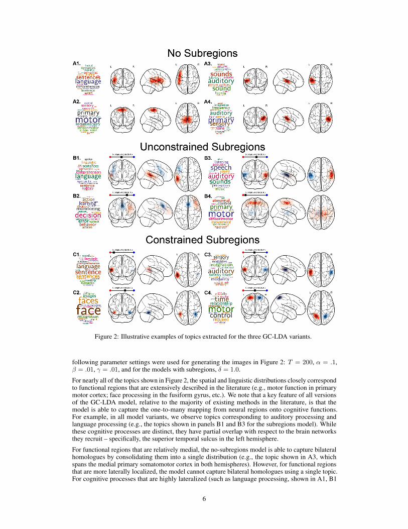
Figure 2: Illustrative examples of topics extracted for the three GC-LDA variants.

following parameter settings were used for generating the images in Figure 2: T = 200, α = .1,β = .01, γ = .01, and for the models with subregions, δ = 1.0.

For nearly all of the topics shown in Figure 2, the spatial and linguistic distributions closely correspondto functional regions that are extensively described in the literature (e.g., motor function in primarymotor cortex; face processing in the fusiform gyrus, etc.). We note that a key feature of all versionsof the GC-LDA model, relative to the majority of existing methods in the literature, is that themodel is able to capture the one-to-many mapping from neural regions onto cognitive functions.For example, in all model variants, we observe topics corresponding to auditory processing andlanguage processing (e.g., the topics shown in panels B1 and B3 for the subregions model). Whilethese cognitive processes are distinct, they have partial overlap with respect to the brain networksthey recruit – specifically, the superior temporal sulcus in the left hemisphere.

For functional regions that are relatively medial, the no-subregions model is able to capture bilateralhomologues by consolidating them into a single distribution (e.g., the topic shown in A3, whichspans the medial primary somatomotor cortex in both hemispheres). However, for functional regionsthat are more laterally localized, the model cannot capture bilateral homologues using a single topic.For cognitive processes that are highly lateralized (such as language processing, shown in A1, B1

6

and C1) this poses no concern. However, for functional regions that are laterally distant and do havespatial symmetry, the model ends up distributing the functional region across multiple topics–see,e.g., the topics shown in A3 and A4 in the no-subregions model, which correspond to the auditorycortex in the left and right hemisphere respectively. Given that these two topics (and many other pairsof topics that are not shown) correspond to a single cognitive function, it would be preferable if theywere represented using a single topic. This can potentially be achieved by increasing the flexibilityof the spatial representations associated with each topic, such that the model can capture functionalregions with distant lateral symmetry or other discontiguous spatial features using a single topic. Thismotivates the unconstrained and constrained subregions models, in which topic’s spatial distributionsare represented by Gaussian mixtures.

In Figure 2, the topics in panels B3 and C3 illustrate how the subregions models are able to handlesymmetric functional regions that are located on the lateral surface of the brain. The lexical dis-tribution for each of these individual topics in the subregions models is similar to that of both thetopics shown in A3 and A4 of the no-subregions model. However, the spatial distributions in B3 andC3 each capture a summation of the two topics from the no subregions model. In the case of theconstrained subregion model, the symmetry between the means of the spatial distributions for thesubregions is enforced, while for the unconstrained model the symmetry is data-driven and falls outof the model.

We note that while the unconstrained subregions model picks up spatial symmetry in a significantsubset of topics, it does not always do so. In the case of language processing (panel A1), thelack of spatial symmetry is consistent with a large fMRI literature demonstrating that languageprocessing is highly left-lateralized [11]. And in fact, the two subregions in this topic correspondapproximately to Wernicke’s and Broca’s areas, which are integral to language comprehension andproduction, respectively. In other cases, (e.g., the topics in panels B2 and B4), the unconstrainedsubregions model partially captures spatial symmetry with a highly-weighted subregion near thehorizontal midpoint, but also has an additional low-weighted region that is lateralized. While thisresult is not necessary wrong per se, it is somewhat inelegant from a neurobiological standpoint.Moreover, there are theoretical reasons to prefer a model in which subregions are always laterally-symmetrical. Specifically, in instances where the subregions are symmetric (the topic in panel B3for the unconstrained subregions model and all topics for the constrained subregions model), thesubregion weights provide a measure of the relative lateralization of function. For example, thelanguage topic in panel C1 of the constrained subregions model illustrates that while there is neuralactivation corresponding to linguistic processing in the right hemisphere of the brain, the function isstrongly left-lateralized (and vice-versa for face processing, illustrated in panel C2). By enforcingthe lateral symmetry in the constrained subregions model, the subregion weights π(t)

r (illustratedabove the left activation images) for each topic inherently correspond to an automated measure of thelateralization of the topic’s function. Thus, the constrained model produces what is, to our knowledge,the first data-driven estimation of region-level functional hemispheric asymmetry across the wholebrain.

3.2 Predicting Held Out Data

This section describes quantitative comparisons between three GC-LDA models in terms of theirability to predict held-out data. We split the Neurosynth dataset into a training and test set, whereapproximately 20% of all data in the corpus was put into the test set. For each document, werandomly removed

⌊.2N

(d)x

⌋peak activation tokens and

⌊.2N

(d)w

⌋word tokens from each document.

We trained the models on the remaining data, and then for each model we computed the log-likelihoodof the test data, both for the word tokens and peak tokens.

The space of possible hyperparameters to explore in GC-LDA is vast, so we restrict our comparisonto the aspects of the model which are novel relative to the original Correspondence-LDA model.Specifically, for all three model variants, we compared the log-likelihood of the test data acrossdifferent values of γ, where γ ∈

{0, 0.001, 0.01, 0.1, 1

}. We note again here that the no-subregions

model with γ = 0 is equivalent to a smoothed version of Correspondence-LDA [2] (see footnote 2for additional clarification). The remainder of the parameters were fixed as follows (chosen based ona combination of precedent from the topic modeling literature and preliminary model exploration):T = 100, α = .1, and β = .01 for all models, and δ = 1.0 for the models with subregions. Allmodels were trained for 1000 iterations.

7

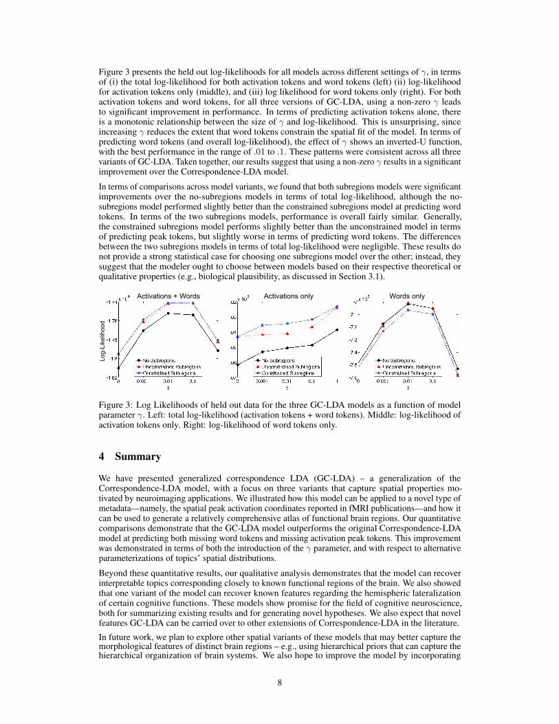
Figure 3 presents the held out log-likelihoods for all models across different settings of γ, in termsof (i) the total log-likelihood for both activation tokens and word tokens (left) (ii) log-likelihoodfor activation tokens only (middle), and (iii) log likelihood for word tokens only (right). For bothactivation tokens and word tokens, for all three versions of GC-LDA, using a non-zero γ leadsto significant improvement in performance. In terms of predicting activation tokens alone, thereis a monotonic relationship between the size of γ and log-likelihood. This is unsurprising, sinceincreasing γ reduces the extent that word tokens constrain the spatial fit of the model. In terms ofpredicting word tokens (and overall log-likelihood), the effect of γ shows an inverted-U function,with the best performance in the range of .01 to .1. These patterns were consistent across all threevariants of GC-LDA. Taken together, our results suggest that using a non-zero γ results in a significantimprovement over the Correspondence-LDA model.

In terms of comparisons across model variants, we found that both subregions models were significantimprovements over the no-subregions models in terms of total log-likelihood, although the no-subregions model performed slightly better than the constrained subregions model at predicting wordtokens. In terms of the two subregions models, performance is overall fairly similar. Generally,the constrained subregions model performs slightly better than the unconstrained model in termsof predicting peak tokens, but slightly worse in terms of predicting word tokens. The differencesbetween the two subregions models in terms of total log-likelihood were negligible. These results donot provide a strong statistical case for choosing one subregions model over the other; instead, theysuggest that the modeler ought to choose between models based on their respective theoretical orqualitative properties (e.g., biological plausibility, as discussed in Section 3.1).

Activations only Words only Activations + Words

Log-

Like

lihoo

d

Figure 3: Log Likelihoods of held out data for the three GC-LDA models as a function of modelparameter γ. Left: total log-likelihood (activation tokens + word tokens). Middle: log-likelihood ofactivation tokens only. Right: log-likelihood of word tokens only.

4 Summary

We have presented generalized correspondence LDA (GC-LDA) – a generalization of theCorrespondence-LDA model, with a focus on three variants that capture spatial properties mo-tivated by neuroimaging applications. We illustrated how this model can be applied to a novel type ofmetadata—namely, the spatial peak activation coordinates reported in fMRI publications—and how itcan be used to generate a relatively comprehensive atlas of functional brain regions. Our quantitativecomparisons demonstrate that the GC-LDA model outperforms the original Correspondence-LDAmodel at predicting both missing word tokens and missing activation peak tokens. This improvementwas demonstrated in terms of both the introduction of the γ parameter, and with respect to alternativeparameterizations of topics’ spatial distributions.

Beyond these quantitative results, our qualitative analysis demonstrates that the model can recoverinterpretable topics corresponding closely to known functional regions of the brain. We also showedthat one variant of the model can recover known features regarding the hemispheric lateralizationof certain cognitive functions. These models show promise for the field of cognitive neuroscience,both for summarizing existing results and for generating novel hypotheses. We also expect that novelfeatures GC-LDA can be carried over to other extensions of Correspondence-LDA in the literature.

In future work, we plan to explore other spatial variants of these models that may better capture themorphological features of distinct brain regions – e.g., using hierarchical priors that can capture thehierarchical organization of brain systems. We also hope to improve the model by incorporating

8

features such as the correlation between topics. Applications and extensions of our approach formore standard image processing applications may also be a fruitful area of research.

References[1] Arthur Asuncion, Max Welling, Padhraic Smyth, and Yee Whye Teh. On smoothing and inference for

topic models. In Proceedings of the Twenty-Fifth Conference on Uncertainty in Artificial Intelligence,pages 27–34. AUAI Press, 2009.

[2] David M Blei and Michael I Jordan. Modeling annotated data. In Proceedings of the 26th annualinternational ACM SIGIR conference on Research and development in informaion retrieval, pages 127–134.ACM, 2003.

[3] David M Blei, Andrew Y Ng, and Michael I Jordan. Latent dirichlet allocation. the Journal of machineLearning research, 3:993–1022, 2003.

[4] Vince D Calhoun, Jingyu Liu, and Tülay Adalı. A review of group ica for fmri data and ica for jointinference of imaging, genetic, and erp data. Neuroimage, 45(1):S163–S172, 2009.

[5] Jeremy R Manning, Rajesh Ranganath, Kenneth A Norman, and David M Blei. Topographic factor analysis:a bayesian model for inferring brain networks from neural data. PloS one, 9(5):e94914, 2014.

[6] Adrian M Owen, Kathryn M McMillan, Angela R Laird, and Ed Bullmore. N-back working memoryparadigm: A meta-analysis of normative functional neuroimaging studies. Human brain mapping, 25(1):46–59, 2005.

[7] Russell A Poldrack, Jeanette A Mumford, Tom Schonberg, Donald Kalar, Bishal Barman, and Tal Yarkoni.Discovering relations between mind, brain, and mental disorders using topic mapping. PLoS Comput Biol,8(10):e1002707, 2012.

[8] Stephen M Smith, Peter T Fox, Karla L Miller, David C Glahn, P Mickle Fox, Clare E Mackay, NicolaFilippini, Kate E Watkins, Roberto Toro, Angela R Laird, et al. Correspondence of the brain’s functionalarchitecture during activation and rest. Proceedings of the National Academy of Sciences, 106(31):13040–13045, 2009.

[9] Bertrand Thirion, Gaël Varoquaux, Elvis Dohmatob, and Jean-Baptiste Poline. Which fmri clustering givesgood brain parcellations? Frontiers in neuroscience, 8(167):13, 2014.

[10] David C Van Essen, Stephen M Smith, Deanna M Barch, Timothy EJ Behrens, Essa Yacoub, Kamil Ugurbil,WU-Minn HCP Consortium, et al. The wu-minn human connectome project: an overview. Neuroimage,80:62–79, 2013.

[11] Mathieu Vigneau, Virginie Beaucousin, Pierre-Yves Herve, Hugues Duffau, Fabrice Crivello, OlivierHoude, Bernard Mazoyer, and Nathalie Tzourio-Mazoyer. Meta-analyzing left hemisphere language areas:phonology, semantics, and sentence processing. Neuroimage, 30(4):1414–1432, 2006.

[12] Tal Yarkoni, Russell A Poldrack, Thomas E Nichols, David C Van Essen, and Tor D Wager. Large-scaleautomated synthesis of human functional neuroimaging data. Nature methods, 8(8):665–670, 2011.

[13] BT Thomas Yeo, Fenna M Krienen, Simon B Eickhoff, Siti N Yaakub, Peter T Fox, Randy L Buckner,Christopher L Asplund, and Michael WL Chee. Functional specialization and flexibility in humanassociation cortex. Cerebral Cortex, page bhu217, 2014.

9

Supplement: Generalized Correspondence-LDAModels (GC-LDA) for Identifying Functional Regions

in the Brain

The notation used for both model specification and inference throughout the supplement is summa-rized in Table 1.

1 Generative Process and Joint Distribution for GC-LDA with GaussianMixtures

For completeness, we present here a modified version of the generative process for the GC-LDAmodel where the spatial distributions are modeled as mixtures of multivariate Gaussians with Rcomponents. We only present the updated process for generating topics t and activation tokens xi, asthe generative process for sampling word tokens wi does not depend on the parameterization of thespatial distributions:

1. For each topic t ∈{

1, ..., T}

:

(a) Sample a Multinomial distribution over word types φ(t) ∼ Dirichlet(β)

(b) Sample a Multinomial distribution over subregions π(t) ∼ Dirichlet(δ)

2. For each document d ∈ {1, ..., D}:

(a) For each peak activation token xi ∈{

1, ..., N(d)x

}:

i. Sample indicator variable yi from Multinomial(θ(d))ii. Sample indicator variable ci from Multinomial(π(yi))

iii. Sample a peak activation token xi from the spatial distribution for subregion r(yi)ci : xi ∼Gaussian(µ(yi)

ci , σ(yi)ci )

The joint distribution of all observed peak activation tokens, word tokens, and latent parameters foreach individual document in the GC-LDA model with a mixture of Gaussian spatial distributions isas follows:

p(x,w, z, y, c, θ) = p(θ|α)·

N(d)x∏

i=1

p(yi|θ(d))p(ci|π(yi))p(xi|µ(yi)ci , σ(yi)

ci

·N

(d)w∏

j=1

p(zj |y(d), γ)p(wj |φ(zj))

(1)

2 Inference for GC-LDA

During inference, we seek to estimate the posterior distribution across all unobserved model pa-rameters. As is typical with topic models, exact probabilistic inference for the GC-LDA model isintractable. Inference for the original Correspondence LDA model [2] used Variational Bayesianmethods. Here, we employ a mixture of MCMC techniques based on Gibbs Sampling [3], sinceGibbs sampling approaches have often outperformed variational methods for inference in LDA [1, 4].

29th Conference on Neural Information Processing Systems (NIPS 2016), Barcelona, Spain.

T R

D NW

γ

w

NX

y

x

θ α

T φβ µ σ

z

D NW

γ

w

NX

y

x

θ α

φβ µ σ

z

π

c

δ

D NW

γ

w

NX

y

x

θ α

T φβ λ1 λN…

z

(A) (B) (C)

Figure 1: (A) Plate notation for the Generalized Correspondence-LDA model, GC-LDA. (B) Platenotation for GC-LDA with spatial distributions modeled as a single multivariate Gaussian (Equivalentto a smoothed version of Correspondence-LDA if γ = 0). (C) Plate notation for GC-LDA withsubregions, with spatial distributions modeled as a mixture of multivariate Gaussians

In describing the inference procedure, we will provide update equations for the three variants ofGC-LDA that were used in our experiments, depicted in Figures 1.B and 1.C. Specifically, wedescribe the updates for the GC-LDA model where each topic’s spatial component is representedby a single Gaussian distribution (Figure 1.B), and for the two GC-LDA models where each topic’sspatial distribution is represented by a mixture of Gaussian distributions (Figure 1.C). As a reminder,the difference between the two versions of the model that use Gaussian mixtures (referred to as the“unconstrained subregions” and “constrained subregions” models), is that we constrain the mean ofthe two Gaussian components to be symmetric with respect to their distance from the origin alongthe horizontal spatial axis in the “constrained subregions” model. In places where the updates forthe versions of the models are different, we will first describe the update for the model with single aGaussian distribution, and then describe how it is modified for the models that use Gaussian mixtures.

After model initialization, our Gibbs Sampling method involves sequentially updating the spatialdistribution parameters Λ(t) for all topics, the assignments zi of word tokens to topics, and theassignments yi of peak activation tokens to topics (and additionally the assignments ci of activationtokens to subregions when using a Gaussian mixture model for each topic’s spatial distribution). Wefirst provide an overview of the sampling algorithm sequence, and then describe in detail the updateequations used at each step. We also note here that the update equations presented here will generalizeto any variant of the GC-LDA model using a single parametric or mixture of parametric spatialdistributions, provided the updates for the spatial parameter estimates are modified appropriately.

2.1 Overview of Inference Procedure

Configuring and running the model consists of two phases: (1) Model initialization, and (2) Inference.We first describe model initialization, and give an overview of the sequence in which model parametersare updated. We will then provide the exact update equations for each of the steps used duringinference.

2.1.1 Model Initialization

To initialize the model, we first randomly assign all yi indicator variables to one of thetopics yi ∼ uniform(1, ..., T ). The zi indicator variables are randomly sampled from themultinomial distribution conditioned on y

(d)i as defined in the generative model: zi ∼

Multinomial( NY D

1d +γ

N(d)x +γ∗T

,NY D

2d +γ

N(d)x +γ∗T

, ...,NY D

Td +γ

N(d)x +γ∗T

). In the model that uses an unconstrained mix-

ture of Gaussians with R = 2, the initial ci are randomly assigned: ci ∼ uniform(1, ...R). In“constrained subregions” model we used a deterministic initial assignment, where we set ci = 1 ifthe x-coordinate of the activation token was less than or equal to zero (i.e., if the activation peak fellwithin the left hemisphere of the brain), and c = 2 otherwise.

2

Table 1: Table of notation used throughout the appendix

Model specificationNotation Meaningwi, xi The ith word token and peak activation token in the corpus

N(d)x , N (d)

w The number of word tokens and peak activation tokens in document d, respectivelyD The number of documents in the corpusT The number of topics in the modelR The number of components/subregions in each topic’s spatial distribution (subregions model)zi Indicator variable assigning word tokens to topicsyi Indicator variable assigning activation tokens to topics

z(d), y(d) The set of all indicator variables for word tokens and activation tokens in document dNY D

td The number of activation tokens within document d that are assigned to topic tci Indicator variable assigning activation tokens to subregions (subregion models)

Λ(t) Placeholder for all spatial parameters for topic tµ(t), σ(t) Gaussian parameters for topic tµ(t)r , σ(t)

r Gaussian parameters for subregion r in topic t (subregion models)φ(t) Multinomial distribution over word types for topic tφ(t)w Probability of word type w given topic tθ(d) Multinomial distribution over topics for document dθ(d)t Probability of topic t given document dπ(t) Multinomial distribution over subregions for topic t (subregion models)π(t)r Probability of subregion r given topic t (subregion models)

β, α, γ Model hyperparametersδ Model hyperparameter (subregion models)

Count matrices used during model inferenceNotation MeaningNY T

t· The number of activation tokens that are assigned via yi to topic t

NY Dtd,−i

The number of activation tokens in document d that are assigned via yi to topic t, excluding theith token

NY D∗zjd

The number of activation tokens in document d that would be assigned to the topic indicated byzj , given the proposed update of yi

NCTrt,−i

The number of activation tokens that are assigned via ci to subregion r in topic t, excluding theith token (subregion models)

NZTwt,−i The number of times word type w is assigned via zi to topic t, excluding the ith token

2.1.2 Parameter Update Sequence

After initialization, the model inference procedure entails repeating the following three parameterupdate steps until the algorithm has converged:

1. For each topic t, update the estimate of the spatial distribution parameters Λ(t) conditionedon the subset of peaks xi with indicator variables yi = t. When using a model withsubregions for the topics’ spatial components, update the estimate of the spatial distributionparameters Λ

(t)r conditioned on the subsets of peaks xi with indicator variables yi = t and

ci = r.

2. For each activation token xi in each document d, update the corresponding indicator vari-able yi assigning the token to a topic, conditioned on the current estimates of all spatialdistribution parameters Λ(·), the current assignments of z(d) of all word tokens to topics indocument d, and the current estimate of the document’s multinomial distribution over topicsθ(d). When using a model with subregions, instead jointly update the indicator variablesyi of the token to a topic and ci of the token to a subregion within topic yi. This update isadditionally conditioned on the current estimate of all topic’s multinomial distributions oversubregions π(·).

3. For each word token wi in each document d, update the corresponding indicator variable ziassigning the token to a topic, conditioned on the current estimates of all topics’ multinomial

3

distributions over words φ(·), and the current assignments y(d) of all peaks to topics indocument d.

Note that we do not need to directly update the θ(d), φ(t) or π(t) parameters during inference, becausethese distributions are “collapsed out” [4] and are estimated directly from the current state of indicatorvariables y, z, and c, respectively. Convergence of this algorithm is evaluated by computing thelog-likelihood of the observed data after every iteration of the sampler; when the log-likelihoodis no increasing over multiple iterations, we halt the algorithm and compute a final estimate of allparameters.

We now provide the update equations for each of these steps.

2.2 Updating Spatial Distribution Estimates: Λ(t)

To estimate the spatial distributions, we compute the maximum likelihood estimates of the spatialdistribution for each topic t, conditioned on the subset of peak activation tokens that are assigned to t:

µ̂(t) =

∑i,yi=t

xi

NY Tt·

(2)

σ̂(t) =

∑i,yi=t

(xi − µ̂(t))2

NY Tt·

(3)

where NY Tt· is the total number of peak activation tokens xi that are assigned (via yi) to t. When

using a mixture of Gaussians for the spatial distributions, the same estimates are used to estimate themeans and covariances for each subregion, µ̂(t)

r and σ̂(t)r , except that the sums are computed over the

subset of peak activation tokens for which yi = t and ci = r.

In the “constrained subregions” model, where the Gaussian component means are constrained to besymmetric about the horizontal spatial axis (with respect to the distance from the origin), we mustfurther modify the estimation procedure. We estimate a single mean for the two subregions, withrespect to it’s location along the horizontal axis in terms of distance from the origin (correspondingto the longitudinal fissure of the brain), by computing the average coordinates of all xi tokensthat are assigned to t after taking the absolute value of the tokens’ distance from the origin. Thisestimate is then used as the mean of the 2nd subregion along the horizontal axis, and the meanof the 1st subregion is set equal to the same mean, reflected about the horizontal axis (so the thatalong this coordinate, µ̂(t)

1 = −µ̂(t)2 ). The covariance matrices of the two subregions are estimated

independently using equation 3.

2.3 Updating Assignments yi of Activation Tokens xi to Topics

The update step, in which peak activation tokens xi to are assigned to topics via the indicator variablesyi, is dependent upon the choice of the spatial distribution. Specifically, when using a model withtopic subregions, this step involves additionally updating the ci assignments of tokens to subregions.We first provide the update equations for the model that uses a single spatial distribution, and thendescribe the modification to this update needed when using a subregion model.

2.3.1 Updating yi Assignments for GC-LDA models with a Single Multivariate GaussianSpatial Distributions

Here, we wish to update the indicator variable y(d)i , which is the assignment of the ith peak ofdocument d to a topic. This update is conditioned on the current estimates of all spatial distributionparameters Λ, the current vector z(d) of assignments of words to topics in document d, and the currentestimate of the document’s multinomial distribution over topics θ(d).

We employ a Gibbs Sampling step to update each indicator variable, using a proposal distribution.The proposal distribution is used to compute the relative probabilities that y(d)i should be assigned to aspecific topic t = 1, ...T . Once the relative probabilities are computed across all topics, we randomlysample a topic-assignment from this proposal distribution, normalized such that the probability ofassigning the word to a topic sums to 1 across all topics. The update equation is as follows:

4

p(yi = t|xi, z(d), y(d)−i ,Λ

(t), γ, α) ∼ p(xi|Λ(t)) · p(t|θ(d)) · p(z(d)|y(d)∗, γ)

∼ p(xi|Λ(t)) · (NY Dtd,−i + α) ·

N(d)w∏

j=1

NY D∗zjd

+ γ

N(d)x + γ ∗ T

(4)

To understand this equation and the notation, let’s consider the three main terms in the equation indetail.

The first term, p(xi|Λ(t)), is simply the probability that peak activation x(d)i was generated from thespatial distribution associated with topic t. For example, if each topic is associated with a singlemultivariate Gaussian distribution, this term corresponds to the multivariate Gaussian probabilitydensity function evaluated at location xi.

The second term, (NY Dtd,−i+α) is an estimate of the probability of sampling topic t from θ(d), using an

estimate of θ(d) that is computed from the set of all indicator variables y(d)−i in document d excluding

the indicator variable for the token i that is currently being sampled. In the notation above, NY Dtd,−i is

equal to the number of peaks in document d that are currently assigned (via the indicator variablesy) to topic t, where −i indicates that the current token that we are sampling is removed from thesecounts. Note that although the actual estimate of θ(d) requires a normalization term, this is notnecessary during Gibbs sampling because the proposal distribution only needs to be proportional tothe true probabilities.

The third term,∏N(d)

wj=1

NY D∗zjd

+γ

N(d)x +γ∗T

is the probability of sampling all of the current indicator variables

z(d) for words in the document, given the count matrixNY D∗ that results from the proposed update ofthe indicator variables for the peak assignment yi. More precisely, this is computing the multinomiallikelihood of generating the current vector of word-topic assignments z(d) for d from the set ofpeak-topic assignments y(d)∗ that would result from the proposed update of yi. In this notation,NY D∗

zjd+γ

N(d)x +γ∗T

is the multinomial probability of sampling the indicator variable zj from the proposed

vector of peak-topic assignments y(d)∗, where NY D∗zjd

is the number of y indicator variables thatwould be assigned to the same topic as indicator variable zj given the proposed update of yi andthe hyperparameter γ (note that this probability is defined in step (b).ii of the generative process).By iterating this product over all indicator variables zj ∈ d, we compute the relative probability ofsampling z(d) from the multinomial distribution defined in the generative model.

2.3.2 Updating yi and ci Assignments for GC-LDA models with a Mixtures of MultivariateGaussian Spatial Distributions

In the GC-LDA model in which each topic’s spatial distribution is a mixture of multivariate Gaussiandistributions, we use a modified Gibbs sampling procedure in which we jointly sample both the yiassignment of the peak activation token to a topic, and the ci assignment of the peak activation tokento a subregion, according to the following update update equation:

p(yi = t, ci = r|xi,z(d), y(d)−i ,Λ

(t), π(t), δ, γ, α)

∼ p(xi|Λ(t)) · p(t|θ(d)) · p(r|π(yi), δ) · p(z(d)|y(d)∗, γ)

∼ p(xi|Λ(t)) · (NY Dtd,−i + α) ·

NCTrt,−i + δ∑R

r′=1(NCTr′t,−i + δ)

·N

(d)w∏

j=1

NY D∗zjd

+ γ

N(d)x + γ ∗ T

(5)

This update equation is the same as the update equation for the model with a single multivariateGaussian distribution per topic, with the exception of the third term, which is estimating the probabilityof sampling the subregion r from topic t. The notation NCT

rt,−i corresponds to the total number ofsubregion indicator variables ci that are currently assigned to subregion r within topic t, excludingthe count of the token that is currently being sampled. As with θ(d) and φ(t), the π(t) parameters

5

don’t need to be explicitly updated. Instead, these are collapsed out, and estimated via the sums ofcounts of the ci indicator variables.

2.4 Updating zi Assignments of Word Tokens wi to topics

Here we wish to update the indicator variables z(d)i , giving the assignment of the ith word token wi indocument d to a topic. This update is conditioned on the current vector y(d) of assignments of peaksto topics in d, and an estimate of each topic’s multinomial distribution over word types φ(t)

This update involves a collapsed Gibbs sampling step similar in form to the one employed forinference in standard LDA [4]. The update equation is as follows:

p(zi = t|wi, z−i, y(d), γ, β) ∼ p(t|y(d), γ) · p(wi|φ(t))

∼ (NY Dtd,−i + γ) ·

NZTwt,−i + β∑T

w′=1(NZTw′t,−i + β)

(6)

The first term in this equation gives the probability of sampling topic t from document d, which isproportional to NY D

td,−i—the count of the number of activation tokens in document d that are currentlyassigned to topic t—plus the smoothing parameter γ, as defined in the generative model. The secondterm in this equation is the probability of sampling word wi from topic t, given the current estimatesof the topic-word multinomial distributions. As with the estimate of θ(d) computed during the yiupdate steps, φ(t) is computed from the counts of word token assignments, where NZT

wt,−i is thenumber of times word type w is assigned to topic t across the vector of indicator variables z−i,ignoring the token that is currently being sampled.

2.5 Computing Final Parameter Estimates

We compute final estimates (as well as estimates to be used for log-likelihood computations duringinference) of the model parameters as follows:

θ̂(d)t =

NY Dtd + α∑T

t′=1(NY Dt′d + α)

(7)

π̂(t)r =

NCTrt + δ∑R

r′=1(NCTr′t + δ)

(8)

φ̂(t)w =

NZTwt + β∑T

t′=1(NZTw′t + β)

(9)

The final estimates for the parameters of the spatial distributions are equivalent to estimates usedduring inference, described previously.

References[1] Arthur Asuncion, Max Welling, Padhraic Smyth, and Yee Whye Teh. On smoothing and inference for topic

models. In Proceedings of the Twenty-Fifth Conference on Uncertainty in Artificial Intelligence, pages27–34. AUAI Press, 2009.

[2] David M Blei and Michael I Jordan. Modeling annotated data. In Proceedings of the 26th annualinternational ACM SIGIR conference on Research and development in informaion retrieval, pages 127–134.ACM, 2003.

[3] Andrew Gelman, John B Carlin, Hal S Stern, and Donald B Rubin. Bayesian data analysis, volume 2.Taylor & Francis, 2014.

[4] Thomas L Griffiths and Mark Steyvers. Finding scientific topics. Proceedings of the National Academy ofSciences, 101(suppl 1):5228–5235, 2004.

6