GDP PER CAPITA IN AFRICA - Central Bank of Nigeria Per Capita in...CBN Journal of Applied Statistics...

CBN Journal of Applied Statistics Vol. 6 No. 1(b) (June, 2015) 219

GDP Per Capita in Africa before the Global Financial Crisis:

Persistence, Mean Reversion and Long Memory Features

Luis A. Gil-Alana1, OlaOluwa S. Yaya

2 and Olanrewaju I. Shittu

3

This paper examined the long memory features of GDP per capita data before

the global financial crisis, using a sample of 26 African countries. The study

employed fractional integration and tested the stability of the differencing

parameter across the sample period for each country. The results indicated

that most of the countries’ GDP series were I(1) or higher. Evidence of mean

reversion was observed in 10 countries where the disturbances were

autocorrelated. There was strong evidence against mean reversion in the

remaining 16 countries. The results also indicated that the fractional

differencing parameter was stable in 17 countries, while the presence of

structural breaks was investigated in the remaining 9 countries.

Keywords: Africa, GDP, Global financial crisis, Long memory, Persistence.

JEL Classification: C22, E23

1.0 Introduction

Long memory and fractional integration are features commonly observed in

macroeconomic time series. In the context of developed countries fractionally

integrated or I(d) models have been widely employed to describe the

behaviour of GDP, real GDP and GDP per capita series in Diebold and

Rudebusch (1989), Haubrich and Lo (1991), Sowell (1992), Beran (1994),

Silverberg and Verspagen (1999), Michelacci and Zaffaroni (2000), Mayoral

(2006) and Caporale and Gil-Alana (2011) among many others. Many of the

above papers deal with convergence and its different variations (real

convergence, beta-convergence, etc.), testing this hypothesis by looking at the

order of integration of the series. Thus, for I(d) models, if d < 1, mean

reversion is obtained and convergence is satisfied. On the other hand, if d = 1

or d > 1, convergence is clearly rejected. The empirical results, at least for the

developed countries, are mixed: some authors found evidence of unit roots in

real output based on standard I(1) techniques (see Mankiw et al., 1992, Quah,

1993, and Sala-i-Martin, 1996). Their approach is based on testing for

convergence in a regression of the first differences of per capita output.

1 Faculty of Economics, University of Navarra, Pamplona, Spain

2 Department of Statistics, University of Ibadan, Ibadan, Nigeria. Corresponding Email:

[email protected], [email protected] 3 Department of Statistics, University of Ibadan, Ibadan, Nigeria

mailto:[email protected]

mailto:[email protected]

220 GDP Per Capita in Africa before the Global Financial Crisis:

Persistence, Mean Reversion and Long Memory Features Gil-Alana et al.

Michelacci and Zaffaroni (2000) have pointed out that this finding cannot be

reconciled with the other stylized facts of unit roots in output (see Nelson and

Plosser, 1982), and a fairly smooth trend of output per capita in the OECD

economies (see Jones, 1995). They show that US per capita output is well

represented by a mean-reverting long memory I(d) process with 0.5 ≤ d < 1,

where d is the fractional integration parameter.

This approach is criticised in Silverberg and Verspagen (2000) who concluded

that the methods are biased in small samples. Instead, Silverberg and

Verspagen (2000) use maximum likelihood approaches, and provide evidence

that fractional integration in the range [0.5, 1), which is a key result in the

paper by Michelacci and Zaffaroni (2000), disappears when these more

appropriate methods are used. In another recent paper, Mayoral (2006)

examined annual real GNP and GNP per capita in the US for the time period

1869-2001, using several parametric and semi-parametric methods. The

results, though slightly different given the technique used, provide evidence

that the orders of integration lie in the interval [0.5, 1), implying

nonstationarity, high persistence and mean-reverting behaviour.

The economic literature on integration theory assumes two distinct positions

relative to the process of country’s growth and the catching up hypothesis.

The first is the theory of country divergence which argues that a higher

integration towards a single currency is expected to increase factor mobility

which can be in favour of the prosperous countries. Therefore, concentration

of economic activity to these attractive countries which dispose more

developed markets and higher level of industrialization can create additional

difficulties to the less developed country and delay their catching up process.

The theory of regional convergence argues that a higher integration will

attenuate the initial regional disparities and in the long run leads to regional

convergence rather than divergence. It further argues that, for example, the

United States of America shows lower regional disparities than the European

Union as a result of deeper economic integration which includes the monetary

integration and common currency. Marques and Soukiazis (1998) investigated

per capita income convergence across countries and regions in the European

Union (EU) using the “sigma” and “beta” convergence approach. They found

different convergence level for each of the data subsamples.

For developing countries, the literature on convergence in GDP is scarce. Real

convergence in some emerging countries has been examined by Cunado et al.


(2004, 2007). Jones (2002) considers the convergence in GDP for a group of

low-income countries in Africa using both cross-sectional and time series

approaches. He concludes that there is convergence among the Economic

Community of West African States (ECOWAS) between 1960 and 1990. He

further states that the speed at which wealthy countries can catch up with the

poor in terms of growth is very slow. Charles et al. (2008) consider real GDP

per capita in the common market for Eastern and Southern Africa from 1950

to 2003 using panel unit root tests. Using this methodology, they find no

evidence of stochastic or conditional convergence in the regions considered.

Joseph (2010) investigates the convergence between a slow growing economy

and a fast growing economy using the case of Ghana as an African country

and UK as a Western European country, accepting the hypothesis of

convergence.

This paper, to the best of our knowledge, is the first to apply fractional

integration techniques in studying convergence among African countries. We

consider the convergence hypothesis in a group of 26 African countries using

their GDP per capita data. Following this section, section 2 briefly describes

the main ideas of the I(d) models. Section 3 presents the data. Section 4

displays the empirical results and Section 5 deals with the robustness of the

results presented. Section 6 concludes the paper.

2.0 The I(d) model

To correctly determine the order of integration in time series is crucial from

both economic and statistical viewpoints. First, we need to introduce some

definitions. Given a covariance stationary process {ut, t = 0, ±1, … }, with

autocovariance function E(ut –Eut)(ut-j-Eut) = γj, we say that ut is integrated of

order 0 if

.lim

T

TjjT

Alternatively, assuming that ut has an absolutely continuous spectral

distribution function, so that it has a spectral density function, denoted by f(λ),

and defined in terms of the autocovariances as

jj jf ,,cos

2

1)(



we say that ut is I(0) if the spectral density function f(λ) is positive and finite

at all frequencies (λ) in the spectrum, i.e.,

.,)(0 allforf

The I(0) models are sometimes called “short memory” due to the fact that, if

there is a degree of association between the observations, this is short and

tends to disappear fast as the distance between the observations increases.

Standard I(0) processes are the white noise and the stationary ARMA

specifications.

Having said this, a process xt is said to be I(d) (and denoted by xt ≈ I(d)) if:

,...,1,0,)1( tuxL tt

d (1)

where L is the lag operator (Lxt = xt-1), d is a real value, and ut is an I(0)

process as defined just above.

The I(d) model with d > 0 belongs to a broader class of models called “long

memory”, which are characterized by the infinite sum of the autocovariances

is infinite, or, alternative, in the frequency domain, because the spectral

density function is unbounded at some point(s) in the spectrum.

The fractional differencing parameter d plays a crucial role from both

economic and statistical viewpoints. Thus, if d = 0 in (1), xt = ut, the process is

I(0) and it could be a stationary and invertible ARMA sequence, when its

autocovariances decay exponentially; however, it could decay at a much

slower rate than exponentially (in fact, hyperbolically) if d is positive.

Moreover, if 0 < d < 0.5, xt is covariance stationary, but its lag-j

autocovariance γj decreases very slowly, at the rate of j2d-1

as j → ∞, and so

the γj are absolutely non-summable. The variable xt is then said to have long

memory given that f(λ) is unbounded at the origin, i.e.,

.as,)(f 01

1 The origin of these processes is in the 1960s, when Granger (1966) and Adelman (1965)

pointed out that most aggregate economic time series have a typical shape where the spectral

density increases dramatically as the frequency approaches zero. However, differencing the

data frequently leads to over-differencing at the zero frequency.


Also, as 𝑑 in (1) increases beyond 0.5 and through 1 (the unit root case), xt

can be viewed as becoming “more nonstationary” in the sense, for example,

that the variance of the partial sums increases in magnitude. Processes of the

form given by (1) with positive non-integer d are called fractionally

integrated, and when ut is ARMA(p, q), xt is known as a fractionally ARIMA

(or ARFIMA) model. This type of model provides a higher degree of

flexibility in modelling low frequency dynamics which is not achieved by

non-fractional ARIMA models. Another interesting distinction is the case of d

< 1 as opposed to 𝑑 ≥ 1. In the former case, the process is mean reverting

with shocks disappearing in the long run. On the contrary, if 𝑑 ≥ 1, mean

reversion does not occur, and the effect of the shocks persists forever in the

series. This is relevant in the context of GDP series noting that a shock in the

series may have a different effect (in the short and in the long run) depending

on the value of the fractional differencing parameter d.

3.0 The data

The data used in this work are based on annual GDP per capita from 1960 to

2006, obtained from International Monetary Fund (IMF). We intentionally

avoided periods of global financial crisis, since these would affect the results

negatively.

Figure 1: Plots of original time series data

ALGERIA BENIN

BOTSWANA BURKINA FASO

BURUNDI CAMEROON

0

1000

2000

3000

4000

1960 20060

100

200

300

400

500

1960 2006

0

1000

2000

3000

4000

5000

6000

7000

1960 20060

100

200

300

400

500

1960 2006



CHAD CONGO

COTE D’ IVOIRE EGYPT

GABON GHANA

KENYA LESOTHO

LIBERIA MALAWI

MAURITANIA NIGER

0

100

200

300

1960 20060

250

500

750

1000

1250

1500

1960 2006

0

250

500

750

1000

1960 20060

1000

2000

3000

1960 2006

0

1000

1960 20060

500

1000

1500

2000

1960 2006

0

1000

2000

3000

4000

5000

6000

7000

8000

1960 20060

150

300

450

600

750

1960 2006

0

150

300

450

600

750

1960 20060

150

300

450

600

750

1960 2006

0

150

300

450

600

1960 20060

50

100

150

200

250

300

1960 2006

0

500

1000

1500

2000

1960 20060

100

200

300

400

500

1960 2006


NIGERIA SENEGAL

SIERRA LEONE SOUTH AFRICA

SUDAN TOGO

UGANDA ZAMBIA

Plots of the time series data are displayed in Figure 1. Along this figure we

can distinguish two different patterns across the countries. On the one hand

we have countries displaying a relatively constant increase across the sample.

Within this group we could include countries such as Benin, Botswana,

Burkina Faso, Egypt, Gabon, Ghana, Kenya, Lesotho, Malawi, Mauritania,

South Africa, Senegal, Togo and Uganda. On the other hand, the remaining

countries (Algeria, Burundi, Cameroon, Chad, Congo, Cote d’ Ivoire, Liberia,

Niger, Nigeria, Sierra Leone, Sudan and Zambia) are characterized by an

oscillating pattern with a substantial decrease during the 90s, and a posterior

increase during the last years in the sample.2 The first 20 sample

autocorrelation values of the first differences for each series were generated,

2 Note, the results of sample autocorrelations were obtained graphically and are available on

request. Also, the Fortran codes written to plot the graphs and compute the fractional

integration parameters are available on request from the authors.

0

100

200

300

400

500

600

700

800

900

1000

1960 20060

100

200

300

400

500

600

700

800

900

1000

1960 2006

0

100

200

300

400

500

1960 20060

1000

2000

3000

4000

5000

6000

1960 2006

0

250

500

750

1000

1250

1500

1960 20060

100

200

300

400

500

1960 2006

0

100

200

300

400

500

1960 20060

250

500

750

1000

1960 2006



and we observed a rapid decrease in the majority of the cases, with most of the

values found within the 95% confidence interval. However, in many of the

series we also observe some significant values away from zero which may

suggest that fractional differentiation (with d smaller or higher than 1) may be

more appropriate than first differences in some cases.

4.0 The empirical results

The first thing we do in this section is to estimate the fractional differencing

parameter d in the model given by equation (1), where xt can be the errors in a

regression model of form:

...,2,1, txty tt (2)

where yt is the observed GDP time series; α and β are the coefficients

corresponding to the intercept and a linear time trend, and based on equation

(1), ut is supposed to be I(0). For this purpose we employ a Whittle function in

the frequency domain. Along with the estimates of α, β and the fractional

differencing parameter d, we also compute the confidence bands of the non-

rejection values of d using the Lagrange Multiplier (LM) procedure of

Robinson (1994). This method tests the null hypothesis:

,: oo ddH (3)

in (1) and (2) for a grid of real-values do. Thus, the null model tested is:

; (1 ) , 1, 2, ...,od

t t t ty t x L x u t

with I(0) ut.

Table 1 displays the estimates of d (along with the 95% confidence band of

the non-rejection values of d using Robinson’s (1994) method) in the model

given by equations (1) and (2) under the assumption that ut in (1) is a white

noise process. Thus, all the time dependence in the process is determined by

the fractional differencing parameter d. We report the estimates of d for the

three standard cases examined in the literature, i.e. a) the case of no regressors

(α = β = 0 in (2)); b) an intercept (α unknown and β = 0); and c) an intercept

with a linear time trend.


Table 1: Estimates of d based on white noise disturbances

*: Evidence of I(d) with d > 1.

***: Evidence of mean reversion (I(d) with d < 1)

We see in Table 1 that independently of the regressors included in the model

the orders of integration are relatively high in all cases. In fact, the estimated

value of d is found to be higher than 1 in the majority of the cases. Evidence

of mean reversion (i.e., an order of integration statistically significantly

smaller than 1) is only found in a single case corresponding to Malawi.3 In a

number of countries (Benin, Sierra Leone, Ghana and Senegal) we also

observe some estimates, which are below 1 though the I(1) null hypothesis

(i.e. d = 1) cannot be rejected at conventional statistical levels. There is an

3 Malawi is the only country where a significant negative value for the first sample

autocorrelation was obtained and that was as a result of overdifferentiation of the first

differenced data. Here, in Table 1, the result of d for the case of Malawi is consistent with the

previous autocorrelations result.

No regressors An intercept A linear time trend

ALGERIA 1.31 (1.14, 1.53)* 1.3 (1.12, 1.52)* 1.29 (1.12, 1.52)*

BENIN 0.88 (0.64, 1.16) 0.79 (0.59, 1.09) 0.81 (0.57, 1.10)

BOTSWANA 1.19 (1.00, 1.61)* 1.19 (1.00, 1.62)* 1.22 (1.00, 1.64)*

BURKINA FASO 1.16 (0.91, 1.46) 1.13 (0.83, 1.47) 1.13 (0.86, 1.48)

BURUNDI 1.19 (1.04, 1.41)* 1.22 (1.09, 1.42)* 1.22 (1.09, 1.42)*

CAMEROON 1.05 (0.86, 1.32) 1.04 (0.85, 1.32) 1.04 (0.86, 1.31)

CHAD 1.41 (1.24, 1.63)* 1.46 (1.25, 1.75)* 1.46 (1.25, 1.76)*

CONGO 1.27 (0.99, 1.58) 1.22 (0.87, 1.55) 1.22 (0.94, 1.54)

COTE D’ IVOIRE 1.25 (0.99, 1.58) 1.25 (0.99, 1.61) 1.25 (0.99, 1.61)

EGYPT 1.29 (0.91, 1.82) 1.17 (0.88, 1.75) 1.18 (0.87, 1.74)

GABON 1.05 (0.76, 1.44) 1.04 (0.73, 1.43) 1.04 (0.79, 1.43)

GHANA 1.18 (0.92, 1.49) 0.96 (0.36, 1.44) 1 (0.79, 1.43)

KENYA 1.35 (1.03, 1.71)* 1.31 (0.85, 1.72) 1.3 (0.93, 1.72)

LESOTHO 1.16 (0.85, 1.55) 1.15 (0.82, 1.57) 1.16 (0.82, 1.57)

LIBERIA 1.25 (1.08, 1.52)* 1.36 (1.17, 1.68)* 1.36 (1.17, 1.68)*

MALAWI 0.51 (0.35, 0.95)*** 0.59 (0.47, 0.90)*** 0.55 (0.36, 0.90)***

MAURITANIA 1.44 (1.04, 1.81) 1.27 (0.51, 1.71) 1.24 (0.80, 1.68)

NIGER 1.17 (0.93, 1.50) 1.23 (0.92, 1.65) 1.22 (0.93, 1.65)

NIGERIA 1.31 (1.09, 1.61)* 1.29 (1.06, 1.61)* 1.29 (1.06, 1.61)*

SENEGAL 1.02 (0.77, 1.34) 0.99 (0.71, 1.37) 1 (0.73, 1.37)

SIERRA LEONE 0.95 (0.74, 1.27) 0.86 (0.64, 1.20) 0.87 (0.66, 1.20)

SOUTH AFRICA 1.2 (0.86, 1.61) 1.19 (0.76, 1.65) 1.19 (0.83, 1.65)

SUDAN 1.07 (0.83, 1.34) 1.01 (0.70, 1.30) 1.02 (0.80, 1.30)

TOGO 1.01 (0.72, 1.42) 1.02 (0.72, 1.45) 1.02 (0.75, 1.45)

UGANDA 1.12 (0.71, 1.54) 1.11 (0.63, 1.57) 1.11 (0.70, 1.57)

ZAMBIA 1.51 (1.22, 1.89)* 1.45 (1.01, 1.92)* 1.43 (1.04, 1.93)*



additional group of countries where the unit root null cannot be rejected,

including Burkina Faso, Cameroon, Congo, Cote d’ Ivoire, Egypt, Gabon,

Lesotho, Niger, South Africa, Sudan, Togo and Uganda. For the remaining

countries (Algeria, Botswana, Burundi, Chad, Kenya, Liberia, Mauritania,

Nigeria and Zambia) the unit root null is decisively rejected in favour of

orders of integration which are above 1. These results are summarized in

Table 2.

Table 2: Summary results from Table 1

*: In these countries the unit root cannot be rejected in some cases.

The results presented so far do not take into account weak autocorrelation for

the error term. This may produce potential biases in the estimated values of d.

A common practice is to employ thee ARMA models for the error term ut in

(1) (Robinson, 1994). However, given the difficulty in determining the

appropriate orders for the AR and MA polynomials, especially in small

samples as is the case in the present work, we use a less conventional

approach due to Bloomfield (1973). This is a non-parametric method, where

the model is implicitly determined by the spectral density function, which is

given by:

m

rr rf

1

22 )(cos2exp

2);(

,

Mean Reversion I(1) behaviour I(d) with d > 1

MALAWI BENIN ALGERIA

BURKINA FASO BOTSWANA

CAMEROON BURUNDI

CONGO CHAD

COTE D’ IVOIRE KENYA*

EGYPT LIBERIA

GABON MAURITANIA*

GHANA NIGERIA

LESOTHO ZAMBIA

NIGER

SENEGAL

SIERRA LEONE

SOUTH AFRICA

SUDAN

TOGO

UGANDA


where σ2 = Var(ϵt) and m is an integer value describing the short run dynamics

of the series. This model produces autocorrelations decaying exponentially as

in the ARMA case, and it accommodates extremely well in the context of the

tests of Robinson (1994) employed in this work.4 Using this approach the

results are presented in Table 3.

Table 3: Estimates of d based on Bloomfield (1973) disturbances

No regressors Intercept Linear time trend

ALGERIA 1.43(0.29, 2.03) 1.30(0.32, 1.95) 1.23(0.48, 1.95)

BENIN 0.48 (0.17, 1.49) 0.52 (0.23, 1.41) 0.43 (-0.27, 1.39)

BOTSWANA 0.46 (0.29, 0.83) ***

0.49 (0.29, 0.90) ***

0.03 (-0.17, 0.53)

BURKINA FASO 0.36 (0.12, 1.45) 0.45 (0.15, 1.35) 0.36 (-0.16, 1.33)

BURUNDI 1.26 (0.89, 1.85) 1.35 (1.02, 1.85)* 1.34 (1.02, 1.82)

*

CAMEROON 0.86 (0.48, 1.42) 0.86 (0.51, 1.40) 0.90 (0.54, 1.37)

CHAD 1.40 (0.81, 1.99) 1.21 (1.00, 1.64)* 0.41 (-0.17, 1.63)

CONGO 0.26 (0.03, 1.64) 0.33 (0.07, 1.54) 0.33 (-0.16, 1.51)

COTE D’ IVOIRE 0.65 (0.23, 1.39) 0.64 (0.31, 1.38) 0.73 (0.34, 1.39)

EGYPT 0.63 (0.47, 0.96) ***

0.73 (0.58, 1.02) 0.30 (-0.14, 1.00)

GABON 0.38 (0.16, 1.05) 0.45 (0.22, 0.97) 0.47 (0.16, 1.02)

GHANA 0.07 (-0.03, 1.53) 0.16 (-0.07, 0.41) ***

-0.07 (-0.34, 0.96) ***

KENYA 0.32 (0.12, 1.78) 0.44 (0.16, 1.70) 0.35 (-0.10, 1.63)

LESOTHO 0.48 (0.27, 1.02) 0.51 (0.30, 0.94) ***

-0.27 (-0.77, 0.95) ***

LIBERIA 1.08 (0.75, 1.54) 1.03 (0.66, 1.53) 1.03 (0.67, 1.51)

MALAWI 0.24 (0.12, 0.45) ***

0.40 (0.19, 0.60) ***

0.19 (-0.10, 0.57) ***

MAURITANIA 0.34 (0.19, 2.44) 0.47 (0.28, 3.00) 0.46 (0.07, 3.05)

NIGER 0.74 (0.13, 1.38) 0.47 (0.14, 1.17) 0.53 (0.18, 1.17)

NIGERIA 0.89 (-0.05, 1.53) 0.58 (-0.08, 1.45) 0.83 (0.19, 1.44)

SENEGAL 0.25 (0.10, 1.23) 0.42 (0.18, 0.92) ***

0.25 (-0.16, 0.93) ***

SIERRA LEONE 0.46 (0.03, 1.07) 0.39 (0.03, 0.89) ***

0.43 (0.05, 0.89) ***

SOUTH AFRICA 0.30 (0.14, 0.61) ***

0.40 (0.18, 0.64) ***

-0.16 (-0.56, 0.53) ***

SUDAN 1.16 (-0.05, 2.14) 1.05 (-0.07, 2.20) 1.04 (-0.01, 2.15)

TOGO 0.28 (0.13, 0.90) ***

0.44 (0.23, 0.83) ***

0.40 (0.08, 0.86) ***

UGANDA 0.09 (-0.04, 0.99)***

0.19 (-0.06, 0.54) ***

-0.20 (-0.62, 0.71) ***

ZAMBIA -0.02 (-0.20, 1.52) -0.03 (-0.30, 1.45) 0.30 (-0.20, 1.33) *: Evidence of I(d) with d > 1.

***: Evidence of mean reversion (I(d) with d < 1)

4 See Gil-Alana (2004) for a paper dealing the model of Bloomfield (1973) in the context of

Robinson’s (1994) tests.



Table 4: Summary results from Table 2

The first noticeable feature in this table is that the confidence intervals are

very large implying that in some cases we cannot reject neither the I(0) nor the

I(1) hypotheses. We also observe in Table 3 that the results differ in some

cases depending on the specification of the deterministic terms. Thus,

evidence of mean reversion is obtained for Botswana (in the cases of no

regressors and with an intercept); Egypt (with no regressors); Ghana, Lesotho,

Senegal and Sierra Leone (with an intercept, and with an intercept and a linear

time trend); and also for Malawi, South Africa, Togo and Uganda (in all

cases). For the remaining countries the results support the existence of unit

roots or orders of integration above 1 (as is the case with Burundi and Chad).

Table 4 summarizes the results displayed in Table 3. We see that mean

reversion is obtained in the cases of Botswana, Egypt, Ghana, Lesotho,

Malawi, Senegal, Sierra Leone, South Africa, Togo and Uganda. Thus, if

autocorrelation is allowed, apart from Malawi, we observe seven additional

countries showing estimates of d which are below 1and thus showing mean

reverting behaviour.

The results presented so far assume that the fractional differencing parameter

has remained constant across the sample period. This is a strong assumption

especially in the context of African countries. In the next section we examine

this issue looking at the stability of d across the sample period.

Mean Reversion I(1) behaviour I(d) with d > 1

BOTSWANA ALGERIA BURUNDI

EGYPT BENIN CHAD

GHANA BURKINA FASO

LESOTHO CAMEROON

MALAWI CONGO

SENEGAL COTE D’ IVOIRE

SIERRA LEONE GABON

SOUTH AFRICA KENYA

TOGO LIBERIA

UGANDA MAURITANIA

NIGER

NIGERIA

SUDAN

ZAMBIA


5.0 Stability tests and robustness checking

Two approaches are implemented here. In the first, we estimate d, for each

country, in a sample for the time period [1960 – 1994]; then we re-estimate d

moving the sample one period forward, i.e., [1961 – 1995] and so on till the

final subsample [1972 – 2006]. Thus, in all cases we consider subsamples of

35 observations each. In the second approach, we start with the same

subsample as in the previous case, adding then one observation each time till

the sample is completed, [1960 – 2006]. The results in terms of the estimation

of d (with their corresponding 95% confidence intervals) are respectively

displayed in Figures 2 and 3.

Figure 2: Results based on moving windows with 35 observations for each

series moving recursively.

ALGERIA BENIN


BURUNDI CAMEROON

CHAD CONGO


0

0,5

1

1,5

2

1 2 3 4 5 6 7 8 9 10 11 12 13

0

0,5

1

1,5

2

1 2 3 4 5 6 7 8 9 10 11 12 13

0

0,5

1

1,5

2

1 2 3 4 5 6 7 8 9 10 11 12 13

0

0,5

1

1,5

2

1 2 3 4 5 6 7 8 9 10 11 12 13

0

0,5

1

1,5

2

1 2 3 4 5 6 7 8 9 10 11 12 13

0

0,5

1

1,5

2

1 2 3 4 5 6 7 8 9 10 11 12 13

0

0,5

1

1,5

2

1 2 3 4 5 6 7 8 9 10 11 12 13

0

0,5

1

1,5

2

1 2 3 4 5 6 7 8 9 10 11 12 13



GABON GHANA

KENYA LESOTHO

LIBERIA MALAWI

MAURITANIA NIGER

NIGERIA SENEGAL


SUDAN TOGO

0

0,5

1

1,5

2

1 2 3 4 5 6 7 8 9 10 11 12 13

0

0,5

1

1,5

2

1 2 3 4 5 6 7 8 9 10 11 12 13

0

0,5

1

1,5

2

1 2 3 4 5 6 7 8 9 10 11 12 13 -0,5

0

0,5

1

1,5

2

1 2 3 4 5 6 7 8 9 10 11 12 13

0

0,5

1

1,5

2

1 2 3 4 5 6 7 8 9 10 11 12 13

0

0,5

1

1,5

2

1 2 3 4 5 6 7 8 9 10 11 12 13

0

0,5

1

1,5

2

1 2 3 4 5 6 7 8 9 10 11 12 13

0

0,5

1

1,5

2

1 2 3 4 5 6 7 8 9 10 11 12 13

0

0,5

1

1,5

2

1 2 3 4 5 6 7 8 9 10 11 12 13

0

0,5

1

1,5

2

1 2 3 4 5 6 7 8 9 10 11 12 13

0

0,5

1

1,5

2

1 2 3 4 5 6 7 8 9 10 11 12 13

0

0,5

1

1,5

2

1 2 3 4 5 6 7 8 9 10 11 12 13

0

0,5

1

1,5

2

1 2 3 4 5 6 7 8 9 10 11 12 13

0

0,5

1

1,5

2

1 2 3 4 5 6 7 8 9 10 11 12 13


UGANDA ZAMBIA

UGANDA ZAMBIA

Looking at the results in Figure 2, we notice ten countries where the estimates

of d remain stable across the sample. They correspond to Algeria, Burkina

Faso, Burundi, Cameroon, Gabon, Kenya, Liberia, Niger, Nigeria and Sierra

Leone. There are three additional countries (Cote d’ Ivoire, Senegal and Togo)

where we observe an initial decrease in the estimate of d though with a

relative stable behaviour across the sample period. In six countries (Chad,

Congo, Egypt, South Africa, Sudan and Zambia) we observe an increase in

the value of d across the sample, and a general decrease is observed in

countries such as Benin, Botswana, Ghana, Lesotho, Malawi and Mauritania.

Figure 3: Results based on moving windows adding one observation each time

to the initial 35 samples

ALGERIA BENIN


0

0,5

1

1,5

2

1 2 3 4 5 6 7 8 9 10 11 12 13

0

0,5

1

1,5

2

1 2 3 4 5 6 7 8 9 10 11 12 13

0

0,5

1

1,5

2

1 2 3 4 5 6 7 8 9 10 11 12 13

0

0,5

1

1,5

2

1 2 3 4 5 6 7 8 9 10 11 12 13

0

0,5

1

1,5

2

1 2 3 4 5 6 7 8 9 10 11 12 13

0

0,5

1

1,5

2

1 2 3 4 5 6 7 8 9 10 11 12 13

0

0,5

1

1,5

2

1 2 3 4 5 6 7 8 9 10 11 12 13

0

0,5

1

1,5

2

1 2 3 4 5 6 7 8 9 10 11 12 13



BURUNDI CAMEROON

CHAD CONGO


GABON GHANA

KENYA LESOTHO

LIBERIA MALAWI

MAURITANIA NIGER

0

0,5

1

1,5

2

2,5

1 2 3 4 5 6 7 8 9 10 11 12 13

0

0,5

1

1,5

2

1 2 3 4 5 6 7 8 9 10 11 12 13

0

0,5

1

1,5

2

1 2 3 4 5 6 7 8 9 10 11 12 13

0

0,5

1

1,5

1 2 3 4 5 6 7 8 9 10 11 12 13

0

0,5

1

1,5

1 2 3 4 5 6 7 8 9 10 11 12 13

0

0,5

1

1,5

2

1 2 3 4 5 6 7 8 9 10 11 12 13

0

0,5

1

1,5

2

2,5

1 2 3 4 5 6 7 8 9 10 11 12 13

0

0,5

1

1,5

2

1 2 3 4 5 6 7 8 9 10 11 12 13

0

0,5

1

1,5

2

1 2 3 4 5 6 7 8 9 10 11 12 13

0

0,5

1

1,5

2

1 2 3 4 5 6 7 8 9 10 11 12 13

0

0,5

1

1,5

2

1 2 3 4 5 6 7 8 9 10 11 12 13

0

0,5

1

1,5

2

1 2 3 4 5 6 7 8 9 10 11 12 13

0

0,5

1

1,5

2

1 2 3 4 5 6 7 8 9 10 11 12 13

0

0,5

1

1,5

2

1 2 3 4 5 6 7 8 9 10 11 12 13


NIGERIA SENEGAL


SUDAN TOGO

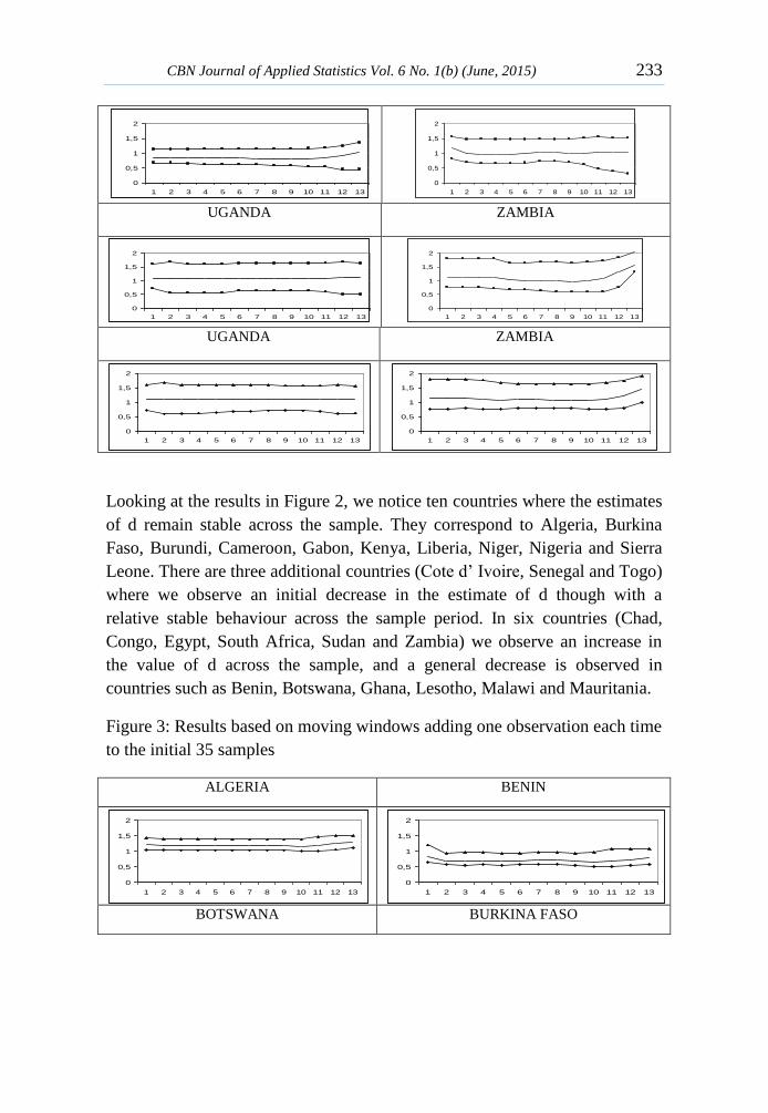
Figure 3 displays the estimates of d adding one observation each time. We

notice in this table that countries like Algeria, Benin, Burkina Faso, Burundi,

Cameroon, Chad, Cote d’ Ivoire, Congo, Gabon, Kenya, Liberia, Niger,

Nigeria, Senegal, Sierra Leone, Sudan and Togo, the estimates of d are very

stable. These countries are the same as those reported in Figure 2 with the

inclusion of Chad, Benin, Congo and Sudan. For the remaining countries, we

observe a reduction in the estimation of d (Botswana, Lesotho and Malawi)

and an increase for Egypt, Ghana, Mauritania, South Africa and Zambia,

which is once more consistent with the results reported in Figure 2.

Due to the small sample sizes of the series examined, it is difficult to draw

conclusions about the existence of breaks. Nevertheless, we have taken the

eight series where we noticed unstable behaviour in the parameter d across

Figure 3 and have looked deeper at its behaviour across the sample period.

0

0,5

1

1,5

2

1 2 3 4 5 6 7 8 9 10 11 12 13

0

0,5

1

1,5

2

1 2 3 4 5 6 7 8 9 10 11 12 13

0

0,5

1

1,5

2

1 2 3 4 5 6 7 8 9 10 11 12 13

0

0,5

1

1,5

2

1 2 3 4 5 6 7 8 9 10 11 12 13

0

0,5

1

1,5

2

1 2 3 4 5 6 7 8 9 10 11 12 13

0

0,5

1

1,5

2

1 2 3 4 5 6 7 8 9 10 11 12 13

0

0,5

1

1,5

2

1 2 3 4 5 6 7 8 9 10 11 12 13

0

0,5

1

1,5

2

1 2 3 4 5 6 7 8 9 10 11 12 13



Table 5: Potential breaks in the series

Table 5 displays in the second column the years of the breaks across the

selected countries, which are Botswana, Lesotho, Malawi, Egypt, Ghana,

Mauritania, South Africa and Zambia. It is observed that in all except one

country (Malawi) there is one single break in the data, which takes place

around 2002/03 in the majority of the series. Only for Ghana and Mauritania

the breaks takes place in the final year of the sample period, 2006. For

Malawi, two breaks are observed, one in 1996 and the other in 2002. If we

focus now on the fractional differencing parameters we notice that for

countries such as Botswana, Lesotho and South Africa, there is a reduction in

the order of integration from values above 1 to values below 1 though the unit

root cannot be rejected in the second estimates; for Malawi, there is a

considerable reduction in the estimation of d, from 0.84 when using the first

subsample (ending at 1996) to 0.63 (with the sample ending at 2002) and to

0.58 (and showing significant evidence of mean reversion) when using the

whole sample period. For the remaining countries (Egypt, Ghana, Mauritania

and Zambia) we observe an increase in the degree of persistence of the series

with the sample.

6.0 Concluding Remarks

In this paper we examine the degree of persistence in the GDP per capita

series in a group of 26 African countries using long range dependence

techniques. We focus on annual data from 1960 to 2006 and the results

indicate that most of the series are highly persistent with orders of integration

equal to or higher than 1. The exceptions are Malawi (if the disturbances in

the d-differenced process are uncorrelated) and Botswana, Egypt, Ghana,

Lesotho, Senegal, Sierra Leone, South Africa, Togo and Uganda, along with

Malawi if the disturbances are autocorrelated. In all these cases mean

Countries Break date(s) d1 d2 d3

BOTSWANA 2003 1.31 (1.09, 1.69) 0.9 (0.76, 1.89) N/A

LESOTHO 2003 1.2 (1.00, 1.47) 0.88 (0.71, 1.44) N/A

MALAWI 1996, 2002 0.84 (0.69, 1.08) 0.63 (0.52, 1.03) 0.58 (0.47, 0.96)

EGYPT 2002 1.08 (0.96, 1.27) 1.15 (0.96, 1.55) N/A

GHANA 2006 0.56 (0.38, 1.35) 0.96 (0.36, 1.44) N/A

MAURITANIA 2006 1.04 (0.74, 1.41) 1.27 (0.51, 1.71) N/A

S. AFRICA 2003 1.09 (0.89, 1.43) 0.8 (0.66, 1.49) N/A

ZAMBIA 2006 1.23 (0.79, 1.75) 1.45 (1.00, 1.92) N/A


reversion may occur to some extent. The stability of the fractional

differencing parameter across the sample is also investigated. The results here

indicate that the parameter d is quite stable in the cases of Algeria, Benin,

Burkina Faso, Burundi, Cameroon, Chad, Cote d’ Ivoire, Congo, Gabon,

Kenya, Liberia, Niger, Nigeria, Senegal, Sierra Leone, Sudan and Togo. In the

remaining countries (Botswana, Egypt, Ghana, Lesotho, Malawi, Mauritania,

South Africa and Zambia) the possibility of a structural break was considered,

and evidence of breaks is found about 2002/03 in the majority of the cases,

noticing a reduction in the degree of persistence for Botswana, Lesotho, South

Africa and Malawi, and an increase for Egypt, Ghana, Mauritania and

Zambia.

This work is limited by the small sample size of the annual time series data

applied. In the future, one can consider applying the quarterly time series to

examine the change in the persistence in GDP per capita before and after the

global crisis.

References

Adelman, I. (1965). Long cycles: Fact or artifacts. American Economic

Review, 55:444-463.

Beran, J. (1994). Statistics for Long Memory Processes, Chapman & Hall,

New York.

Bloomfield, P. (1973). An exponential model in the spectrum of a scalar time

series. Biometrika, 60:217-226.

Caporale, G.M and L.A. Gil-Alana (2011). Long memory in US real output

per capita. CESifo Working Paper Series n. 2671.

Charles, A., O. Darne and J.F. Hoarau (2008). Does the real GDP per capita

convergence hold in the common market for Eastern and southern

Africa? CERESUR, University of LaRe’union.

Cunado, J., L.A. Gil-Alana and F. Perez de Gracia (2004). Real convergence

in some emerging countries: A fractional long memory approach.

Recherches Economiques du Lovain 73(3):293-310.

Cunado, J., L.A. Gil-Alana and F. Perez de Gracia (2007). Real convergence

in Taiwan. A fractionally integrated approach, Journal of Asian

Economics 14(1):119-135.



Diebold, F.X. and G.D. Rudebusch (1989). Long memory and persistence in

the aggregate output. Journal of Monetary Economics 24:189-209.

Gil-Alana, L.A. (2004). The use of the model of Bloomfield as an

approximation to ARMA processes in the context of fractional

integration, Mathematical and Computer Modelling 39:429-436.

Granger, C.W.J. (1966). The typical spectral shape of an economic variable.

Econometrica, 37:150-161.

Haubrich, J.G. and A.W. Lo (1991). The sources and nature of long term

memory in aggregate output. Economic Review of the Federal Reserve

Bank of Cleveland 37:15-30.

Jones, C. (1995). Time series tests of endogenous growth models, Quarterly

Journal of Economics, 110:495-525.

Jones, B. (2002). Economic integration and convergence of per capita income

in West Africa. African Development Bank, pp. 18-47.

Joseph, B. A. (2010). Ghana’s economic growth in perspective: A time series

approach to convergence and growth determinants. Munich Personal

RePEc Archive. Paper no. 23455.

Mankiw, N., D. Romer and D. Weil (1992). A contribution to the empirics of

growth, Quarterly Journal of Economics, 107(2):407-437.

Marques, A. and E. Soukiazis (1998). Per capita income convergence across

countries and across regions in the European Union. Some new

evidence. A paper presented at 2nd

International meeting of European

Economy organized by CEDIN (ISEG), Lisbon.

Mayoral, L. (2006). Further evidence on the statistical properties of real GNP.

Oxford Bulletin of Economics and Statistics 68:901-920.

Michelacci, C. and P. Zaffaroni (2000). (Fractional) Beta convergence.

Journal of Monetary Economics 45(1):129-153.

Nelson, C. and C. Plosser (1982). Trends and random walks in

macroeconomic time series: some evidence and implications, Journal

of Monetary Economics, 10:139-162.


Quah, D. (1993). Empirical cross-section dynamics in economic growth,

European Economic Review, 37(2/3):426-434.

Robinson, P.M. (1994). Efficient tests of nonstationary hypotheses, Journal of

the American Statistical Association 89:1420-1437.

Sala-i-Martin, X. (1996). The classical approach to convergence analysis,

Economic Journal, 106:1019-1036.

Silverberg, G. and B. Verspagen (1999). Long memory in time series of

economic growth and convergence, Eindhoven Center for Innovation

Studies, Working Paper 99.8.

Silverberg, G. and B. Verspagen (2000). A note on Michelacci and Zaffaroni

long memory and time series of economic growth, ECIS Working

Paper 00 17 Eindhoven Centre for Innovation Studies, Eindhoven

University of Technology.

Sowell, F. (1992). Modelling long run behaviour with the fractional ARIMA

model. Journal of Monetary Economics 29:277-302.

GDP PER CAPITA IN AFRICA - Central Bank of Nigeria Per Capita in...CBN Journal of Applied Statistics...

Documents

Transcript of GDP PER CAPITA IN AFRICA - Central Bank of Nigeria Per Capita in...CBN Journal of Applied Statistics...