Latent Estimation of GDP, GDP per capita, and … Estimation of GDP, GDP per capita, and Population...
48
Latent Estimation of GDP, GDP per capita, and Population from Historic and Contemporary Sources Christopher J. Fariss Department of Political Science University of Michigan [email protected] * Charles D. Crabtree Department of Political Science University of Michigan [email protected] Therese Anders School of International Relations University of Southern California [email protected] Zachary M. Jones Department of Political Science Penn State University [email protected] Fridolin J. Linder Department of Political Science Penn State University [email protected] Jonathan N. Markowitz School of International Relations University of Southern California [email protected] * Contact Author. We thank Pablo Barberá, Michael Beckley, Kristian Gleditsch, James Lo, and Mark Major for helpful comments on this project. All data and code necessary to replicate the model and predicted data presented in the article will be publicly available upon publication at dataverse repositories maintained by the authors. This research was supported in part by The McCourtney Institute for Democracy Innovation Grant, and the College of Liberal Arts, both at Pennsylvania State University and the Security and Political Economy (SPEC) Lab at the University of Southern California. 1 arXiv:1706.01099v1 [stat.AP] 4 Jun 2017
Transcript of Latent Estimation of GDP, GDP per capita, and … Estimation of GDP, GDP per capita, and Population...

Latent Estimation of GDP, GDP per capita, andPopulation from Historic and Contemporary Sources
Christopher J. FarissDepartment of Political Science
University of [email protected] ∗
Charles D. CrabtreeDepartment of Political Science
University of [email protected]
Therese AndersSchool of International RelationsUniversity of Southern California
Zachary M. JonesDepartment of Political Science
Penn State [email protected]
Fridolin J. LinderDepartment of Political Science
Penn State [email protected]
Jonathan N. MarkowitzSchool of International RelationsUniversity of Southern California
∗Contact Author. We thank Pablo Barberá, Michael Beckley, Kristian Gleditsch, James Lo, and MarkMajor for helpful comments on this project. All data and code necessary to replicate the model and predicteddata presented in the article will be publicly available upon publication at dataverse repositories maintainedby the authors. This research was supported in part by The McCourtney Institute for Democracy InnovationGrant, and the College of Liberal Arts, both at Pennsylvania State University and the Security and PoliticalEconomy (SPEC) Lab at the University of Southern California.
1
arX
iv:1
706.
0109
9v1
[st
at.A
P] 4
Jun
201
7

Abstract
The concepts of Gross Domestic Product (GDP), GDP per capita, and populationare central to the study of political science and economics. However, a growing litera-ture suggests that existing measures of these concepts contain considerable error or arebased on overly simplistic modeling choices. We address these problems by creating adynamic, three-dimensional latent trait model, which uses observed information aboutGDP, GDP per capita, and population to estimate posterior prediction intervals foreach of these important concepts. By combining historical and contemporary sourcesof information, we are able to extend the temporal and spatial coverage of existingdatasets for country-year units back to 1500 A.D through 2015 A.D. and, becausethe model makes use of multiple indicators of the underlying concepts, we are ableto estimate the relative precision of the different country-year estimates. Overall, ourlatent variable model offers a principled method for incorporating information fromdifferent historic and contemporary data sources. It can be expanded or refined asresearchers discover new or alternative sources of information about these concepts.
Keywords: Gross Domestic Product, population, GDP per capita, latent variables,measurement, construct validity
2
Introduction
The concepts of Gross Domestic Product (GDP), GDP per capita (GDPpc), population, or
some combination of the three rest at the heart of many political and economic theories of
interstate and intrastate behaviors. Since GDP, population, and GDP per capita are strongly
related to many important factors, social scientists often include measures of these concepts in
their empirical analyses. In some cases, researchers are substantively interested in estimating
the effect of these variables on an outcome of interest (e.g., Gilpin 1981; Kennedy 1987;
Przeworski et al. 2000; Charron and Lapuente 2010). Others make the explanation of the
growth of population, GDP, or GDP per capita the focal point of their research (e.g., North
1990; Mankiw et al. 1992; Galor 2005; Acemoglu and Robinson 2012). In many other cases,
researchers include these measures to control for cross-country differences in population or
the size of the economy.1 Yet, despite the vital role that these variables play in empirical
social science, there are theoretical reasons to believe that they are measured imprecisely.
Indeed, a growing literature suggests that existing measures of these important quantities
contain considerable error (Jerven, 2010c,b,a, 2013b, 2014; UNU-IHDP and UNEP, 2014;
Wallace, 2016). These errors could substantially affect the inferences we make about these
variables on other social phenomena either directly or indirectly (Stefanski and Carroll, 1985;
Wooldridge, 2010).
In this paper, we address this construct validity issue by creating and making available
new estimates of GDP2, GDP per capita3, and population.4 The estimates are obtained by1This occurs despite the concern that including these variables in statistical analyses could introduce post-
treatment bias, as they might be measured after the outcome of interest has occurred (Przeworski, 2009).King (2006) points out, “this is an important point that is often missed” (124). The consequence of this biasis that it can prevent causal interpretations of estimated coefficients (King and Zeng, 2007).
2For observed data on GDP see World Bank (2016); Broadberry and Klein (2012); Maddison (2010);Gleditsch (2002); Bairoch (1976).
3For observed data on GDP per capita see World Bank (2016); Broadberry (2015); The Maddison-Project(2013); Broadberry and Klein (2012); Gleditsch (2002); Bairoch (1976).
4For observed data on population see World Bank (2016); Broadberry and Klein (2012); Maddison (2010);
3
combining multiple sources of information for each of these concepts in a dynamic, three-
dimensional latent trait model. These measures improve on alternatives in several important
ways. First, the dynamic latent variable model extends the temporal and spatial coverage of
existing measures by combining information from contemporary and historical sources. The
resulting estimates extend from 1500 A.D. to 2015 A.D., the most recent year the observed
data are available.5 Second, because the estimates make use of multiple indicators of the
underlying concepts, we are able to estimate the relative precision of the different country-
year values for each of the observed measures included in the model. The model provides a
complete set of historical estimates for these three latent variables in the form of prediction
intervals for thousands of previously missing country-year units in addition to prediction
intervals for the original observed country-year variables themselves.6 Information from these
country-year prediction intervals can be incorporated into empirical models that estimate the
relationship between these variables and other variables of historic or contemporary interest.
Finally, because the models are used to generate predictive intervals for the original source
data, the new estimates are available for scholars in the unit-of-measurement of the original
observed variables. The resulting dataset covers 35,299 country-year units, for which 16,145
of these country-year units were previously missing. Overall, because the latent variable
model offers a principled method for incorporating information from different historic and
contemporary data sources and estimating unit specific uncertainty, it can be expanded or
refined as other researchers discover new or alternative data sources of these concepts or
other information about the recording and reporting processes themselves. We demonstrate
Gleditsch (2002); Singer et al. (1972).5A country enters the dataset in 1500 A.D. or the first year in which at least one of the datasets records
a value for at least on of the included variables (e.g., England 1500-2015 A.D.; Argentina 1800-2015 A.D.;Ghana 1820-2015 A.D.).
6Missing values are inferred from the dynamic structure of the model based on the information containedin the variables associated with a given country year and the estimates from prior and future values.
4

this feature of the model using historic data for Ghana.
Before discussing the latent variable model and its estimates, we review the known sources
of error in existing measures. Next we describe the GDP, GDP per capita, and population
variables. We then introduce the dynamic measurement model and describe how it incor-
porates information from these three sets of variables. After that, we assess the construct
validity of the posterior predictive intervals by comparing them to the observed variables.
We close with a discussion of several possible extensions of the model.
Sources of GDP, GDP per capita, and Population Measurement Error
Existing measures of GDP, GDP per capita, and population attempt to quantify three related
constructs. Gross Domestic Product (and the related Gross National Product) are intended to
measure the total amount of the economic output created in a country in a given year (World
Bank, 2016). Population measures are intend to reflect the total number of people within the
geographic unit in a given year (World Bank, 2016). GDP per capita (and the related GNP
per capita) is a measure of the total amount of the economic output created in a country
per person in a given year (World Bank, 2016). The empirical constructs that are intended
to map on to these theoretical concepts suffer from a fundamental measurement problem
— they are incompletely observable and must be inferred from economic source material
and census information. It is extremely labor intensive and cost prohibitive to count every
individual within most administrative units (e.g., municipalities, counties, provinces, states)
or to track every unit of wealth created in a country (GDP) or by a country’s firms (GNP)
each year. This means that these empirical constructs can only be estimated each year and
that some degree of error will always be present in the resulting variable values available in
a country’s available statistical material. While there must be some error in how they are
measured, a large and growing literature suggests that current measures contain considerable
5

error and that it is possibly even systematically related to the estimation process itself (a
point we return to in the conclusion) (e.g., Jerven, 2010c,b,a, 2013b, 2014; Wallace, 2016).
As Jerven (2013b) shows, there are many reasons for this measurement error. One source
of error is that states have strategic incentives to release biased statistics (Wallace, 2016).
On one hand, states might have reason to over-report official statistics. This is because
high population and GDP numbers might increase domestic support, impress the govern-
ments of other states, or gain the attention of foreign investors. The Chinese government,
for example, appears to exaggerate its official estimates to forestall opposition criticism and
thereby improve regime support (Wallace, 2016). A similar logic allegedly motivates the Be-
larusian government to release what are known to be very conservative emigration estimates
(Yeliseyeu, 2014). The widely circulated rumor is that state leaders do not want the public
to know that many Belarusians find other countries more attractive homes. States might
also under-report official statistics. This is because low population and GDP numbers might
attract foreign aid (Neumayer, 2003; Burnside and Dollar, 2000) or other forms of interna-
tional assistance (Büthe et al., 2012). These strategic incentives might lead to systematic
reporting errors in the source material used to construct the data (Fariss, 2014; Scott, 1998).
Another issue is that states do not, or cannot, collect accurate data. Even countries with
a well developed census bureaucracy face political issues in accurately counting all groups
with the same level of accuracy (Prewitt, 2010). The situation is worse in some parts of
the developing world, where population estimates are often outdated simply because many
countries do not or cannot conduct a regular census (e.g., Discoll and Lidow, 2014). The
absence of a regular census might be because states are not interested in gathering these data
or because they do not have the capacity to do so. Regardless of the cause, the result is the
same — outdated data for many country-year observations.
Similarly, GDP estimates are often outdated because countries do not update their ‘base
6

year’ regularly (Data Quality Institute, World Economics, 2016). In certain years, statisti-
cians collect additional data on the structure of a country’s economy (Jerven, 2013a). These
years, called ‘base years,’ are then used to weigh the relative contribution of those sectors
to the national income (Jerven, 2013b). The contribution of sectors can change considerably
over time, as new industries emerge and old ones disappear (Jerven, 2013a, 141-144). As
a result, the United Nations and International Monetary Fund both recommend that states
‘rebase’ their estimates every five years to capture changes in the influence of sectors within
countries (Jerven, 2013a; Data Quality Institute, World Economics, 2016). Many countries,
however, update this quantity less frequently than suggested. For example, a recent survey
suggests that only 7 of 48 countries in sub-Saharan Africa follow this recommendation (Jer-
ven, 2013a, 146). When these countries do eventually update this quantity, it can lead to
substantial changes in GDP estimates. For example, Nigeria garnered attention in 2013 when
an update to its base year resulted in an 89 percent increase of its GDP estimate for that
year (Economist, 2014). As this case illustrates, using old base years can cause considerable
error in reported GDP estimates.
In addition to these shared sources of error, there are many other factors that specifically
influence the accuracy of GDP estimates. One such factor relates to the United Nations
System of National Accounts (SNA or UNSNA) (European Communities et al., 2009). The
SNA is a set of international recommendations about measuring economic activity, designed
to make cross-national comparisons easier (Deaton and Heston, 2010; Data Quality Institute,
World Economics, 2016). The recommendations are updated semi-regularly (e.g., (United
Nations, 1953; European Communities et al., 2009)). However, not all states use these
standards and many that do might not use the most up to date version (Data Quality
Institute, World Economics, 2016). This leads to considerable heterogeneity across countries
in the degree to which reported GDP statistics capture underlying economic activity as
7

reflected by a standardized reporting procedure.
Another factor that can lead to misreporting is the size of a country’s informal, or
shadow, economy. This sector of the economy comprises a mix of legal activities, such
as self-employment and bartering, and illegal activities, such as drug-dealing and gambling
(Schneider and Enste, 2000, 5). In developing countries, the informal market can represent
a substantial share of the economy — perhaps more than 40 percent (International Labour
Office, 2013). Even in OECD countries, it can represent about 15 percent of all activity
(International Labour Office, 2013). While states usually try to incorporate informal work in
their national statistics, this can be difficult since it requires accurately calculating the value
of this work (Schneider and Enste, 2000).
A third additional factor that can lead to error in GDP estimates is whether and how
states account for public sector outputs (Atkinson, 2005). There are two issues here. One
is that the national accounts system in most states only tracks government inputs, such as
salaries and fixed costs, but not government outputs, such as education and welfare services
(Stiglitz et al., 2009, 31). By not accounting for government outputs, states underestimate
national economic activity (Stiglitz et al., 2009). Another issue is that governments often
subsidize the cost of public goods, leading to sub-market prices for these goods (Stiglitz et al.,
2009, 17). As a result, states that measure government outputs based on their market value
also underestimate national economic activity.
Despite these sources of error, and the potential dangers they pose to empirical work, there
have been few attempts to systematically account for them across all available data sources.7
Most efforts to improve population and GDPmeasures have focused on extending their spatial
or temporal coverage (which we are interested in as well). These projects typically ‘fill in’7These has been substantial work on understanding the error in government statistics for a subset of
countries and years, particularly in countries in Africa (e.g., Jerven, 2010a,b,c, 2013b, 2014).
8

gaps from country-year series that were the result of conflict or political instability (Gleditsch,
2002). Perhaps the most prominent example of this is the historic GDP and population
dataset constructed by Angus Maddison (Maddison, 2010; The Maddison-Project, 2013).
While these efforts have been extremely useful, as reflected in the thousands of citations they
have received, they do not directly address our primary concern, which is the existence of
bias and error in reported country-year estimates. While this line of research has focused
on providing researchers with more data, we add to this contribution by both extending the
coverage of the estimates temporally and spatially and also by providing researchers with a
means of understanding the relative precision of the resulting estimates.
Several organizations, such as World Economics (Data Quality Institute, World Eco-
nomics, 2016), have tried to address the concern we raise about these statistics by releasing
datasets that measure their quality. There are two primary problems with these datasets,
however. The first is that their temporal range is usually extremely limited. The second
is that while these measures provide some information about the relative uncertainty of of-
ficial GDP statistics, they do not incorporate this information into country-year estimates.
Our new model and model-based estimates, which we describe below, provide a method for
addressing these limitations. Importantly, our model should be considered a useful starting
point that can be extended as new information becomes available. We discuss several such
extensions and provide one demonstration using information from the case of Ghana (Jerven,
2014).
9

GDP, Population, and GDPpc Component Datasets
Our latent variable model is estimated based on data for Gross Domestic Product (GDP)8,
GDP per capita9, and population.10 Details on the sources, measurement choices, and cov-
erage of the component variables are provided in Table 1. For each component dataset,
we extract relevant indicators, attach unique country identifiers, and reshape the data into
a common country-year format. We consulted the codebooks of each dataset to drop ob-
servations that are interpolated or extrapolated by the authors of the dataset, or already
covered by other datasets (e.g., the data generated by Gleditsch (2002) includes some in-
terpolated values and values taken from the Maddison Project). Details on the underlying
source materials for each component measure and coding decisions are provided below and
are documented in the R code we use to merge the constituent datasets together.
When merging the different variables together we relied on the available country-year units
as prepared by the authors of the original datasets. We use the Gleditsch and Ward (1999)
revised list of independent states as the base set of units. For years prior to the start year of
this data set (1816 A. D.) we again use the date the year the unit enters the dataset or 1500
A.D. As we discussed in each dataset description, different datasets sometimes use different
spatial definitions for units. We have matched country-year units across datasets using the
best match available. In some cases, units exist in the dataset that are not historically
accurate such as a unified Germany prior to 1871. Maddison includes this unit in his historic
data series, aggregating information across the various principalities and other administrative
districts that existed until Germany had completely unified in 1871. As another example,8For observed data on GDP see World Bank (2016); Broadberry and Klein (2012); Maddison (2010);
Gleditsch (2002); Bairoch (1976).9For observed data on GDP per capita see World Bank (2016); Broadberry (2015); The Maddison-Project
(2013); Broadberry and Klein (2012); Gleditsch (2002); Bairoch (1976).10For observed data on population see World Bank (2016); Broadberry and Klein (2012); Maddison (2010);
Gleditsch (2002); Singer et al. (1972).
10
Maddison also disaggregates information about North and South Korea backwards in time.
Additional details about these unit specific issues are available in the original source material.
Documentation about how we merged all of the data sources together are available in our
code files, which are publicly accessible. Importantly, because many of these units are subsets
of larger ones (e.g., North and South Korea), analysts can aggregate the estimates of these
two units together if necessary for a specific empirical application.
11

Table 1: Component Measures for GDP, GDP per capita, and PopulationLatent Variable Model
Variable Descriptions Coveragein Original
Coveragein Model
Source Material and Citations
GDP data are measured in 1990 internationaldollars.
1AD–2008 1500–2008 Historical GDP data collected by AngusMaddison (Maddison, 2010).
GDP data are measured as total real GDP at2005 prices.
1950-2011 1950-2011 Expanded GDP data version 6.0 beta,September 2014 (Gleditsch, 2002).
GDP data are measured in constant 2010 USD. 1960–2015 1960–2015 World Development Indicators (WorldBank, 2016)
GDP data limited to European countries and theUnited States, after accounting for changingcountry boundaries. GDP is measured in millionsof 1990 international dollars (national currenciesare converted to international dollars usingAngus Maddison’s purchasing power parities)
1870–2001 1870–2001 Broadberry and Klein (2012).
GNP data limited to European countries, afteraccounting for changing country boundaries.GNP is measured at market prices and expressedin constant 1960 US dollars.
1830–1973 1830–1973 Bairoch (1976).
GDP per capita data are measured in 1990international dollars.
1AD-2010 1500–2010 Extension of Angus Maddison’s historicalGDP and population estimates (TheMaddison-Project, 2013).
GDP per capita data are measured as total realGDP at 2005 prices.
1950-2011 1950-2011 Expanded GDP data version 6.0 beta,September 2014 (Gleditsch, 2002).
GDP per capita are measured in constant 2010USD.
1960–2015 1960–2015 World Development Indicators (WorldBank, 2016)
GDP per capita data limited to Europeancountries and the United States, after accountingfor changing country boundaries. GDP ismeasured in millions of 1990 international dollars.
1870–2001 1870–2001 Broadberry and Klein (2012).
GNP per capita data are limited to Europeancountries, after accounting for changing countryboundaries. GNP is measured at market pricesand expressed in constant 1960 US dollars.
1830–1973 1830–1973 Bairoch (1976).
GDP per capita data limited England/GreatBritain, Holland/Netherlands, Italy, Spain,Japan, China, and India. GDP is measured inmillions of 1990 international dollars.
725–1850 1500–1850 Broadberry (2015).
Total population measured in thousands atmid-year.
1AD–2030 1500–2010 Historical population data collected byAngus Maddison (Maddison, 2010).
Total population measured in thousands. 1950-2011 1950-2011 Expanded GDP data version 6.0 beta,September 2014 (Gleditsch, 2002).
Population data limited to European countriesand the United States.
1870–2001 1870–2001 Broadberry and Klein (2012).
Total population. 1960–2015 1960–2015 World Development Indicators (WorldBank, 2016)
Total population measured in thousands. 1816–2001 1816–2001 The Correlates of War Project’s NationalMaterial Capabilities data version 4.0(Singer et al., 1972)
12

The Maddison Project (Maddison, 2010; The Maddison-Project, 2013)
Maddison’s original GDP, GDP per capita, and population variables are derived from a
large number of country-level sources (Maddison, 2003, 2001, 1995). Because the underlying
source materials employed by Maddison are expansive and country-specific, we refrain from
describing them in detail. The more recent version of these data, The Maddison-Project
(2013), is based on a collaboration of researchers dedicated to continuing Angus Maddison’s
data collection efforts by extending and, if warranted, revising his estimates. Due to the
collaborative nature of the effort, different research teams use different methods and source
material to obtain their estimates. With a few exceptions, data from 1990–2010 were revised
using figures from the Total Economy Database of the Conference Board (Bolt and van
Zanden, 2014). Other estimates are based on historical national statistics from country-
specific sources (Bolt and van Zanden, 2014). We subset the data from the Maddison Project
to include only country-year observations starting in 1500. The original Maddison (2010)
data includes both GDP and population values. The updated version only included GDP
per capita estimates. We include both data versions in our model since, as we describe below,
it is capable of linking all of these observed indicators together in united model that leverages
the information from each type of variable. Unlike some of the other datasets we describe
below, these datasets do not contain origin codes that classify the source material used to
inform the country-year values.
Expanded GDP data version 6.0 beta (Gleditsch, 2002)
Gleditsch (2002)’s (beta) version 6.0 of the Expanded GDP data is based primarily on the
13

Penn World Tables (PWT) 8.0, and supplemented with data from the PWT 5.6, the Mad-
dison Project Database, and the World Bank Global development indicators. In addition,
Gleditsch (2002) constructed his data using imputations for the lead and tail values, as well
as interpolation for estimates within the series. We use only the values that stem from the
PWT figures in the latent variable model (origin codes 0, -1, and 3) and exclude data from
the Maddison Project, as well as interpolated or imputed figures (origin codes -2, 1, and 2).
In the Validity section below, we consider the model fit for the latent variables estimates
that do include these variables compared to the latent variable model estimates that exclude
them and demonstrate the model fit is improved by estimating these missing values using
our model-based approach instead of using interpolation or extrapolation.
World Development Indicators (World Bank, 2016)
We include GDP, GDP per capita, and population from the World Bank (2016). Where
possible, we use the metadata for each indicator provided by the World Bank’s DataBank to
determine the underlying source material of the GDP, GDP per capita, and population values.
As with the Gleditsch (2002) data, we drop values that are interpolated or extrapolated and
allow our model to generate new estimates for these units. We describe each of these variables
in turn.
We include the World Bank (2016)’s GDP indicator measured in constant 2010 US dollars
in our latent variable model. The figures are compiled from the World Bank and OECD
national accounts data. The documentation in the metadata file indicates that the series is
based on an underlying interpolation of component data upon aggregating it to a “gap-filled
total.” Unfortunately, we do not have information on the details of this aggregation process.
We therefore use the full series of GDP as provided by the World Bank (2016)’s online data
portal DataBank. In future versions of our model, we plan to identify these cases when
14

possible and adjust our model accordingly.
The per capita GDP series is based on the World Bank (2016)’s GDP in constant 2010
US dollars and the total population figures (for the underlying source material see below).
According to the metadata, the data is aggregated using weighted averages. We exclude
observations from our model that the metadata indicates as being preliminary, extrapolated,
or interpolated. Information on which country-years were excluded based on the metadata
is provided in the replication material that accompanies this paper.
The population figures from World Bank (2016) are based on national population cen-
suses. The census data that informs this measure stem from a variety of sources, including
the United Nations World Population Prospects (for the majority of developing countries),
Eurostat (for European countries), and national statistical agencies. The data are interpo-
lated for all years between census years. Since we do not have information on the years that
a census was conducted for each country, we retain the interpolated data for the use in the la-
tent variable model. We do, however, exclude population figures that are explicitly indicated
as being extrapolated, interpolated, or preliminary in the metadata. Information on which
country-years-units were excluded is provided in the replication material that accompanies
this paper. In future versions of our model, we plan to identify the other interpolated cases
when possible and again adjust our model accordingly.
Broadberry and Klein (2012)
The GDP, GDP per capita, and population variables in Broadberry and Klein (2012) are
limited to European nations, including Russia and Turkey, as well as the United States. A
detailed list of underlying source material is available in the paper’s appendix (Broadberry
and Klein, 2012, pp. 105). For GDP, these sources include the data from Maddison (2010),
official national account statistics, and the work of country-expert historians. Data on pop-
15
ulation are drawn mainly from Mitchell (2003) and Maddison (2010), and supplemented
with country-specific data from official national statistics and historians. We exclude those
country-year observations that are taken from Maddison (2010) in our model.
Bairoch (1976)
The underlying source material for the data by Bairoch is detailed in the paper’s method-
ological appendix. For GNP, these sources include the work of historians and official national
statistics for earlier country-years, as well as OECD figures for years starting in 1950 (Bairoch,
1976, 329 et seq.). For the 19th century and the year 1900, three-year annual averages are
available for every decade starting from 1830 and expressed in 1960 U.S. dollars (Bairoch,
1976, 286). For the 20th century, data are available for select years between 1913 and 1973 and
expressed in 1960 U.S. dollars as well (Bairoch, 1976, 297). For population, Bairoch relies on
United Nations Demographic yearbooks, data from the League of Nations, and national sta-
tistical agencies to assemble his data (321). We incorporate all of Bairoch’s estimates in our
model, including the ones flagged as having a larger-than-average margin of error (the figures
presented in parentheses). The data from Bairoch (1976) cover the total and per capita gross
national product (GNP), not gross domestic product (GDP). Bairoch’s definition is based
on the United Nations’ 1953 System of National accounts (United Nations, 1953). With the
exception of the data from Bairoch (1976), the data on economic size are measured as the
gross domestic product (GDP). Bairoch (1976) uses gross national product (GNP) instead.
While the GNP excludes value added by foreign firms, this measure is highly correlated with
GDP, as demonstrated in Table 5 in the Appendix. The correlation between GNP and GDP
is quite high, with correlation coefficients between 0.865 and 0.995 for country-year units
within the period 1830–1973. The strength of the positive relationship varies over time but
rarely falls below 0.9. We anticipate that in future years, the correlation between the two
16

measures should drop as globalization increases and the internationalization of production
and investment increases the relevance of the conceptual difference between GNP and GDP.
Additional estimates of GNP and GDP from more recent years would help researchers deter-
mine how this empirical relationship evolves over time. The evaluation of this distinction is
one possible avenue that our new latent variable model opens up for exploration, which we
discuss below.
Broadberry (2015)
The GDP per capita estimates in Broadberry (2015) are based on historical national account-
ing data that is constructed from documents such as “government accounts, customs accounts,
poll tax returns, parish registers, city records, trading company records, hospital and edu-
cational establishment records, manorial accounts, probate inventories, farm accounts, tithe
files and other records of religious institutions.” (Broadberry, 2015, 5). Broadberry lists the
data sources for each country in the main text.11 As with the Maddison data, we exclude
cases for years prior to 1500 from our model.
COW National Military Capabilities data v4.0 (Singer et al., 1972)
The Correlates of War Project provides a variety of country-level estimates including popula-
tion beginning in the year 1816. For country-years starting in 1919, the population estimates
by Singer et al. (1972) are based primarily on the estimates of the United Nations Statistical
Office. The population estimates for years prior to 1919 are based on national government
censuses. For these earlier years in the series, the authors of the population dataset selected
country-specific data that presents the greatest continuity with the data from the United11Pages 6 and 7 contain the underlying source material for Britain, the Netherlands, Italy, and Spain; page
8 contains the data for China, Japan, and India.
17

Nations.12 The authors of the data use a variety of methods to bridge gaps in the data,
including interpolation, regression, and extrapolation. Quality codes for the estimates of
the total population figure are specified — indicating whether a data point stems from an
identified source, is missing, derived through interpolation, regression, or extrapolation. We
retain only those data points that stem from an identified source (quality code A).
Model Description, Specification, and Estimation
The empirical goal for this paper is to specify a dynamic latent variable model that will allow
us to leverage the available information across different contemporary and historical sources
of data on GDP, population, and GDP per capita. Unlike other latent variable models, we
are not directly interested in the estimated latent traits. Instead we use these estimated
traits to generate prediction intervals for each of the observed variables in their original unit-
of-measurement. The model therefore allows us to leverage the information across all of the
observed data and to generated predictions for each of the individual observed variables.
In this way, interested users can select their preferred dataset for empirical applications
in conjunction with the prediction intervals generated from our model. Importantly, the
prediction intervals are available for every unit included in the dataset. As we discuss later
in the manuscript, the size of the prediction interval is related to total coverage and agreement
of the observed variables.
To specify the dynamic latent variable model, let i = 1, . . . , N , index cross-sectional units
and t = 1, . . . T , index time periods. For each country-year unit, j = 1, . . . , J indexes the ob-
served variables yitj. Because the observed variables that enter the model represent three dif-
ferent concepts — GDP, population, and GDP per capita — we estimate three latent variable12For details, please refer to the codebook for version 4.0 of the data: Correlates of War Project Na-
tional Material Capabilities Data Documentation Version 4.0, http://cow.dss.ucdavis.edu/data-sets/national-material-capabilities/nmc-codebook/at_download/file, accessed 1 December 2016.
18

parameters, where k = 1, 2, 3, indexes the three categories gdp, pop, gdppc. This allows us to
define the set of yitj that we observe for each of the k dimensions of the latent variable model,
where yitj ∗1{y ∈ πk}. This notation allows us to denote the set of observed variables used to
estimate each of the three underlying latent variables such that πgdp = {yit1, yit2, yit3, yit4, yit5},
πpop = {yit6, yit7, yit8, yit9, yit10}, πgdppc = {yit11, yit12, yit13, yit14, yit15, yit16}.13
With knowledge of how the observed variables relate to each category k, we can denote
how the three dimensions of the latent variable relate to them as well. The model assumes
that the latent variables take the form: θitk ∼ N (0, 1) for all i when t = 1 (the first year a
country enters the dataset). When t > 1, the standard normal prior is centered around the
latent variable estimate from the previous year such that: θitk ∼ N (θit−1,k, σk).
The latent variables themselves are estimated with uncertainty. The first year each coun-
try enters the model, the variances for these parameters are set to 1. For all years after t = 1,
σgdp and σpop are drawn from a uniform distribution U(0, 1). For the latent GDP per capita
variable, the latent estimates and associated uncertainty are deterministically determined
by the GDP and Population latent variables themselves such that θit,gdppc ← θit,gdpθit,pop
. This
modeling innovation allows information form the three types of observed variables to inform
more than just one of the latent variables.
The latent variables are estimated by linking each of these parameters to the sets of
observed GDP, population, or GDP per capita variables. Since all of the GDP, population,
and GDP per capita variables are continuous, we specify a Gaussian link function with
a unique error term for each of the the three types of variables τk: {τgdp, τpop, τgdppc}.
These τk parameters are estimates of model level uncertainty, which link each of the latent13A useful feature of this notation is that the sets of observed variables do not need to be mutually exclusive.
Though we do not allow the observed variables to inform the estimation of multiple latent variables in theapplication presented here, this is a possibility in other applications. See Gelman and Hill (2007); Imai et al.(2017) for more details. We thank James Lo for this notational suggestion.
19

variables to the sets of observed GDP, population, or GDP per capita variables. Shape
parameters translate the observed variables from their original unit-of-measurement into the
latent variable unit-of-measurement. Because we specify a Gaussian link function, these shape
parameters are the intercept and slope from the linear model. For the intercept parameters
αj, we center the standard normal prior around the the mean value of the observed data with
a relatively large variance (low precision): αj ∼ N (yj, 4). We choose the mean value of the
observed variables because the mean of latent traits themselves are centered around 0.14 The
intercept parameter therefore transforms the latent trait into the unit-of-measurement of the
original observed variable. For identification of the model we set βj = 1 because we assume a
one-unit change in the latent trait is equivalent to a one-unit change in the original observed
variable.15 All of the prior distributions are summarized in Table 2. Recall that we organize
the three types of observed variables in three sets such that yitj ∗ 1{y ∈ πk}. Therefore, the
likelihood function that links the observed data to the estimated parameters is:
L(β, α, τ, θ|yitj ∗ 1{y ∈ πk}) =N∏i=1
T∏t=1
J∏j=1
K∏k=1
N (αj + θitkβj, τk)
The model is estimated with five MCMC chains, run for 100,000 iterations each. The
first 50,000 iterations were thrown away as burn-in and the rest were used to generate the
posterior prediction intervals for the original observed variables.16
14We set this parameter to the empirical mean of the Maddison GDP and population variables as anidentification constraint.
15This assumption can be relaxed to examine the relative strength of the relationship between one measurecompared to another. We leave this analysis to future research. Relaxing this assumption would allow foranalysts to explore the relative relationship between measures of GDP and GNP as functions of the underlyinglatent trait. We view this as a useful extension to the model we present here.
16The Gibbs sampler was implemented in Martyn Plummer’s JAGS software (Plummer, 2010). The JAGScode used is displayed in the Appendix. Conventional diagnostics all suggest convergence.
20

Table 2: Prior Distribution for Latent Variables and Model Level Parameter Estimates
Parameter PriorCountry i latent GDP estimate in first year t θit=1,gdp ∼ N (0, 1)Country i latent GDP estimate in all other years θit,gdp ∼ N (θt−1,gdp, σgdp)Latent GDP uncertainty σgdp ∼ U(0, 1)
Country i latent population estimate in first year t θit=1,pop ∼ N (0, 1)Country i latent population estimate in all other years θit,pop ∼ N (θt−1,pop, σpop)Latent population uncertainty σpop ∼ U(0, 1)
Country i latent GDP per capita estimate θit,gdppc ← θit,gdpθit,pop
Model j intercept “difficulty parameter” αj ∼ N (yitj , 4)Model j slope “discrimination parameter” βj ← 1
Model uncertainty for all GDP items τgdp ∼ G(0.001, 0.001)Model uncertainty for all population items τpop ∼ G(0.001, 0.001)Model uncertainty for all GDP per capita items τgdppc ∼ G(0.001, 0.001)
21

Model Validity Checks
Convergent Validity
To assess the validity of the new estimates, we first check for convergent validity. We do this
by comparing the posterior prediction intervals and the observed variables we used to estimate
the latent traits. Figure 1 displays the relationship between the original observed variables
(yitj), the mean or expected value of the latent trait estimates (E(θitk)), and the mean or
expected value of the posterior prediction intervals (E(yitj)). The plot demonstrates the high
level of agreement between the original observed variables and the new posterior predictions.
Figure 2 illustrates this agreement for each observed variable and its corresponding posterior
predictions. Conveniently for users, the posterior predicted values are estimated using the
original unit-of-measurement (e.g., the natural log of 1990 International Dollars). This means
that the visual discrepancy, for example between the World Bank (2016) and the other
population data, is not an empirical one. Instead, it is simply the difference in the unit-of-
measurement used for the observed values (i.e., the World Bank (2016) publishes the absolute
GDP and population values while others present these per thousand individuals).
22

Figure 1: The figure presents the pairwise correlations between all component variables ofthe latent variable model, their estimates, and the latent variables for GDP, per capita GDP,and population. The shading indicates the value of the correlation coefficient [−1, 1]. Whitecells with a value of NA denote pairings with no overlapping country-year observations. Notethat cells that round up to 1 but are not exactly 1 (i.e. all cells that are not in the diagonal),are represented as 0.99.
23

Figure 2: The plot illustrates the agreement between the observed country-year-variablevalues (orange boxes) and the posterior predicted point estimates for which the observedvalue is missing (light grey boxes). Dark grey boxes show the distribution for the full rangeof the posterior predicted point estimates (including estimates for which the original value ismissing). Across all variables, these estimated values have a lower median value due to a biasin the missingness in the original data. We have more missing observations in earlier years, forwhich GDP, per capita GDP, and population levels are lower than in later years in the series.Conveniently for users, the posterior predicted values are estimated using the original unit-of-measurement. This means that the visual discrepancy, for example between the WorldBank (2016) and the other population data, is not an empirical discrepancy. It is simplythe difference in the unit-of-measurement used for the observed values (i.e., the World Bank(2016) publishes the absolute GDP and population values while others present these in perthousand units). Table 3 quantifies the similarity between the original data and the full rangeof possible values along the posterior predicted range, demonstrating that approximately 86percent of the observed country-year-variable values are within ± 1 standard deviation of thepredicted range of the estimated data. 24

Precision of Estimates
As we discussed above, the underlying latent traits themselves are estimated with uncertainty.
Conveniently, the amount of uncertainty for any particular observation is available for each
posterior predicted unit. This information should be incorporated into any analysis that
utilizes these new estimates (Schnakenberg and Fariss, 2014).
Theoretically, the precision of our posterior estimates should increase with the amount
of information (i.e. number of component measures) available for each country year. Figure
3 illustrates the relationship between the amount of information — the number of observed
variables per country-year unit — and the level of uncertainty for each country-year estimate
of the latent variable. As the number of observed pieces of information increases, the level
of uncertainty decreases. Because the latent variable model is dynamic, even country-year
units with 0 observed variables have some information — the latent variable estimate from
the prior year — with which to estimate a value of the latent variable. We use these intervals
to estimate the precision of the new posterior predictions relative to the original observed
variable.
To assess the precision of the new posterior predictions relative to the original observed
variable we estimate a country-year unit Z-score. Because the original variables and the pre-
dicted variables are both continuous, interval-level, and normally distributed, we are able to
compare the original observed country-year unit variable’s position relative to the country-
year unit distribution of the posterior predicted interval. The Z-score’s value represents the
positions of the observed variable’s value relative to the center of the posterior predicted in-
terval. A value of 0 indicates that the observed variable’s value falls directly at the center of
the posterior predicted interval. Z-score units above and below the 0 represent standard de-
viation differences from the center value of the posterior predicted interval. We can therefore
use these values to get a sense of how close the observed value for each country-year vari-
25

able is to its corresponding posterior predicted interval. The country-year-variable Z-score
values take the form: zitj =yitj−E(yitj)
σyitj, where yitj is the observed value for the country-year-
variable, E(yitj) is the expected value or mean for the posterior predicted interval, and σyitj
is the standard deviation for the posterior predicted interval.
Table 3 quantifies the similarity between the original data and the full range of possible
values for the posterior predicted range using the country-year-variable Z-scores zitj. Ap-
proximately 86 percent of the observed country-year-variable values are within ± 1 standard
deviation of the predicted range of the estimated data. We can visualize these patterns as
well. The level of uncertainty over time is visible in time series plots for each of the new pos-
terior predictions for 14 different countries (see Figure 4, 5, and 6). These figures illustrate
the high level of agreement between the original observed variables and the new posterior
prediction intervals. These intervals are much larger for country-year units without data as
well as country-year units with fewer observed values. Overall, the new estimates closely ap-
proximate the original data, but do not always agree. These areas of disagreement between
original observed variable and posterior prediction represent useful deviant cases that can
inform future research (e.g., Lijphart, 1971; Seawright and Gerring, 2008).
26
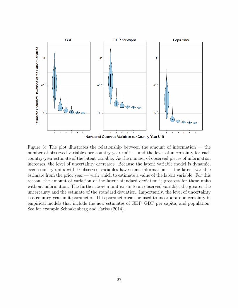
Figure 3: The plot illustrates the relationship between the amount of information — thenumber of observed variables per country-year unit — and the level of uncertainty for eachcountry-year estimate of the latent variable. As the number of observed pieces of informationincreases, the level of uncertainty decreases. Because the latent variable model is dynamic,even country-units with 0 observed variables have some information — the latent variableestimate from the prior year — with which to estimate a value of the latent variable. For thisreason, the amount of variation of the latent standard deviation is greatest for these unitswithout information. The further away a unit exists to an observed variable, the greater theuncertainty and the estimate of the standard deviation. Importantly, the level of uncertaintyis a country-year unit parameter. This parameter can be used to incorporate uncertainty inempirical models that include the new estimates of GDP, GDP per capita, and population.See for example Schnakenberg and Fariss (2014).
27
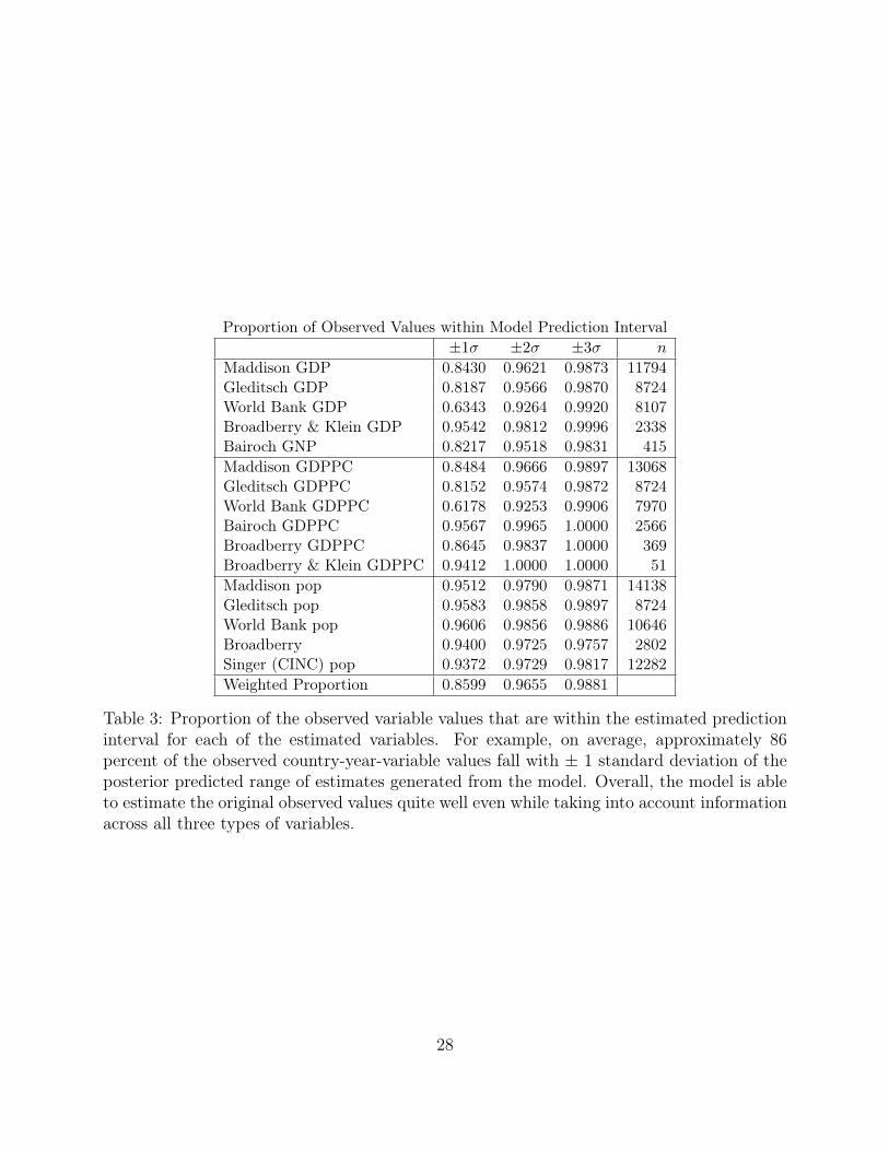
Proportion of Observed Values within Model Prediction Interval±1σ ±2σ ±3σ n
Maddison GDP 0.8430 0.9621 0.9873 11794Gleditsch GDP 0.8187 0.9566 0.9870 8724World Bank GDP 0.6343 0.9264 0.9920 8107Broadberry & Klein GDP 0.9542 0.9812 0.9996 2338Bairoch GNP 0.8217 0.9518 0.9831 415Maddison GDPPC 0.8484 0.9666 0.9897 13068Gleditsch GDPPC 0.8152 0.9574 0.9872 8724World Bank GDPPC 0.6178 0.9253 0.9906 7970Bairoch GDPPC 0.9567 0.9965 1.0000 2566Broadberry GDPPC 0.8645 0.9837 1.0000 369Broadberry & Klein GDPPC 0.9412 1.0000 1.0000 51Maddison pop 0.9512 0.9790 0.9871 14138Gleditsch pop 0.9583 0.9858 0.9897 8724World Bank pop 0.9606 0.9856 0.9886 10646Broadberry 0.9400 0.9725 0.9757 2802Singer (CINC) pop 0.9372 0.9729 0.9817 12282Weighted Proportion 0.8599 0.9655 0.9881
Table 3: Proportion of the observed variable values that are within the estimated predictioninterval for each of the estimated variables. For example, on average, approximately 86percent of the observed country-year-variable values fall with ± 1 standard deviation of theposterior predicted range of estimates generated from the model. Overall, the model is ableto estimate the original observed values quite well even while taking into account informationacross all three types of variables.
28

Figure 4: Gross Domestic Product posterior prediction intervals (grey lines) and observedvariables (orange points). Approximately 86 percent of the observed country-year-variablevalues fall with ± 1 standard deviation of the posterior predicted range of estimates generatedfrom the model.
29

Figure 5: Gross Domestic Product per capita posterior prediction intervals (grey lines) andobserved variables (orange points). Approximately 86 percent of the observed country-year-variable values fall with ± 1 standard deviation of the posterior predicted range of estimatesgenerated from the model.
30
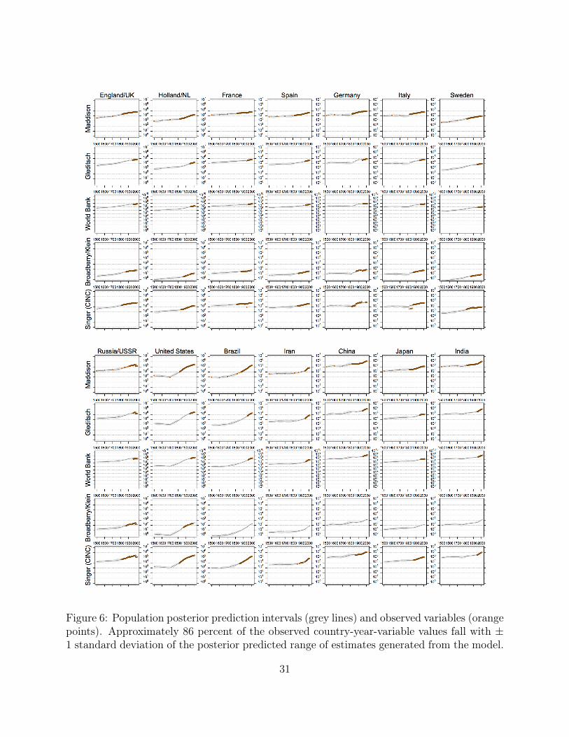
Figure 6: Population posterior prediction intervals (grey lines) and observed variables (orangepoints). Approximately 86 percent of the observed country-year-variable values fall with ±1 standard deviation of the posterior predicted range of estimates generated from the model.
31

Identifying Bias in Component Measures
We have already demonstrated that the number of observed variables is related to the level
of uncertainty for each country-year estimate of the latent variable and the level of uncer-
tainty around the posterior prediction intervals (see Figure 3). We also illustrated how this
manifests using the Z-score estimates zitj to show how closely the prediction interval is to
the observed value for each country-year-variable observation. However, as additional vari-
ables are observed for a given country-year unit we begin to observe bias with respect to the
distance between the observed value of a given variable and the posterior prediction interval
as evidenced by the value of zitj. These statistics allow us to gain insight into how the latent
variable model accounts for disagreement between the observed variables.
Figure 7 illustrates the relationship between the number of observed variables and the
level of agreement between the original country-year variable value and the posterior predicted
intervals for country-year units for which we observed the labeled variable in addition to +0
to +4 of the additional variables. The five rows of panels represent the country-year units
with 1 to 5 observed variables (+0 to +4 additional observed variables). When only one of
the original variables is observed for a given country-year unit, we see that both the level
of uncertainty is relatively high (see Figure 3) and the distance between the observed value
and prediction interval is relatively close (see Figure 7). That is, for country-year units with
only 1 observed variable, the Z-scores are centered over 0 and the standard deviations for
the posterior predicted values are relatively high. These two patterns change as additional
variables are observed for a given country-year unit. For the small number of country-year
units that are covered by 4 or 5 of the available variables, we begin to see some substantial
differentiation between the prediction intervals and the observed values. The values for zitj
are nearly all different than 0 for these country-year units. This is especially apparent for the
observed values from the World Bank variables. According to the model based estimates, the
32

original observed values from the World Bank are systematically higher than the posterior
prediction intervals, though the observed values still tend to fall within 2 standard deviations
of these intervals. The values from the variables from the other datasets tend to fall below
the median prediction but are within 1 standard deviation of the intervals.
Overall, as more information becomes available for a particular country-year unit, the
latent variable model becomes increasingly certain about the value of the estimated posterior
prediction interval (σyitj decreases). However, as the number of observed values increases we
can begin to identify systematic differences between the original data and our new posterior
predicted estimates. These country-year units in particular are useful cases to study because
they may represent places where information is collected in different ways or where other
data production biases might be introduced into some of the constituent datasets we have
brought together. The underlying reasons for these systematic differences are useful starting
points for future scholarship. One advantage of our model, is that it identifies these areas
when there is sufficient coverage across available datasets.
33

Figure 7: This figure illustrates the relationship between the number of observed variablesand the level agreement between the original country-year variable value and the posteriorpredicted intervals for country-year units for which we observed the labeled variable in addi-tion to 0 to 4 of the additional variables. The five rows of panels represent the country-yearunits with 1 to 5 observed variables (0 to 4 additional variables). For a small number ofcountry-year units that are covered by 4 or 5 of the available variables, we begin to see somesubstantial differentiation between the prediction intervals and the observed values.
34

Improving Model Fit with Knowledge of the Original Data
With knowledge about the origin of the original observed data, we can assess the value added
of our model compared to some other methods used to generate estimates for units that are
missing observations. Several of the observed datasets (Gleditsch, 2002; Singer et al., 1972;
World Bank, 2016) provide information about the methods used to infer missing values using
interpolation or extrapolation. In all of the models we have discussed so far, we have removed
these interpolated or extrapolated values in order to let our model predict them. Table 4
displays the difference in root-mean-square error (RMSE) comparing model predictions for
several of these variables between two versions of the latent variable model. The models are
identical except that in the primary model, units with interpolated or extrapolated values
are changed to missing for each variable when those units are identified within the source
material that accompanies the original dataset. Smaller RMSE statistics indicate that, when
the interpolated or extrapolated values are present, that they increase the uncertainty in the
estimates for those units that were observed from primary or secondary sources materials
(i.e., those values that were not interpolated or extrapolated).
Only the five variables included in this table have accompanying information, which
indicates which units are not drawn from primary sources documents and are estimated
instead. Overall, the evidence indicates that for three of these five variables (all of the
population variables), the latent variable model predictions achieve better model fit when
the interpolated and extrapolated values are set to missing. Additional auxiliary information
about the data sources and potential biases of specific country-year units might help to
further improve the model-based estimates. The model we have developed is extendable and
can accommodate such information as it becomes available.
35

Diff 95% Credible Int Pr(Diff)
World Bank pop -0.015 [-0.018, -0.013] 1.000Gleditsch GDP 0.001 [-0.007, 0.009] 0.363Gleditsch GDPPC 0.001 [-0.006, 0.008] 0.374Gleditsch pop -0.013 [-0.016, -0.010] 1.000Singer (CINC) pop -0.006 [-0.009, -0.004] 1.000
Table 4: Difference in root-mean-square error (RMSE) comparing model predictions forseveral variables between two versions of the latent variable model. The models are identicalexcept in one model, units with interpolated values are changed to missing for each variablewhen those units are identified within the source material that accompanies the originaldataset. Smaller RMSE statistics indicate that the interpolated or extrapolated values areincreasing the uncertainty in the estimates of the units without interpolated or extrapolatedvalues. Only the five variables included in this table have accompanying information, whichindicates which units are not drawn from primary sources documents but are estimatedinstead. Overall, the evidence indicates that for three of these five variables (all of thepopulation variables), the latent variable model predictions achieve better model fit whenthe interpolated and extrapolated values are set to missing.
36

Extending the Model with Unit Specific Information: The Case of Ghana
Jerven (2014) provides new estimates of GDP growth in the Gold Coast and Ghana using
sources from the British colonial administration. The information is historically of interest
because of the large number of primary source documents that account for the period before,
during, and after a major cocoa boom, which is not picked up by available data. This
extension illustrates how a country-specific analysis can help to augment the latent variable
model that we described above.
Because the growth rate is a deterministic transformation of GDP, we can include observed
information on this concept in the model developed above. To extend the model we add a
fourth category k : ∆gdp and a new set of observed indicators for this new category such
that π∆gdp = {yit17). yit17 is the growth rate variable for Ghana taken from Jerven (2014).
We set α17 to 0 because the growth rate variable is very close to centered around 0 and
we do not need to scale it. Just like the GDP per capita latent variable, the new growth
rate latent variable is a deterministic transformation of other latent variables in the model.
Specifically, we link these new growth rate data to the latent GDP variable in years t and
t− 1, using the form θit,∆gdp ← θit,gdpθit−1,gdp
− 1. The likelihood equation remains unchanged with
these additions to the latent variable model.17 With this expanded parameterization, we can
now leverage the growth rate data collected by Jerven (2014) to improve the estimation of the
GDP, and GDP per capita latent variables for this country. Figure 8 shows the improvement
in the Ghana specific GDP time series. From 1891 through the 1950s, the economy in Ghana
fluctuated and grew rapidly before eventually slowing after the boom in cocoa production.
These historic changes are now captured in the time series for Ghana and replicate the point
estimates produced by Jerven (2014). We can now illustrate these changes directly and how
they change the GDP trend over time.
17We also estimate an additional τ∆gdp parameter.
37
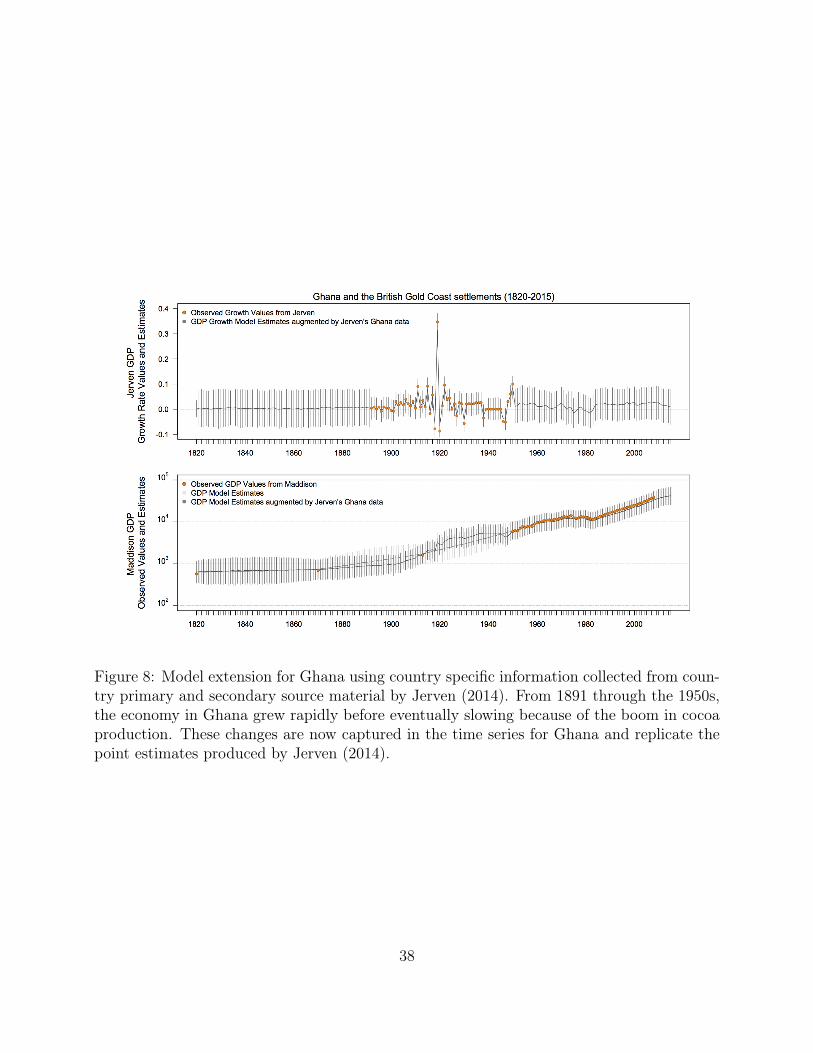
Figure 8: Model extension for Ghana using country specific information collected from coun-try primary and secondary source material by Jerven (2014). From 1891 through the 1950s,the economy in Ghana grew rapidly before eventually slowing because of the boom in cocoaproduction. These changes are now captured in the time series for Ghana and replicate thepoint estimates produced by Jerven (2014).
38

Conclusion
In this paper, we identified and discussed the limitations of existing GDP, GDP per capita,
and population variables. We then introduced and described a new latent variable model
that estimates posterior predictions for these important concepts. These new estimates pro-
vide several primary advantages over existing measures: (1) they extend the temporal and
spatial coverage of existing measures, (2) they include multiple manifest indicators of each
concept, (3) they quantify the uncertainty for each of the country-year estimates. In addi-
tion to the new estimates, the latent variable model itself provides a principled avenue for
exploring the relationship between new data and existing data. To close, we outline several
possible extensions of our latent variable model. To encourage the extension of our model,
we make publicly available the data and code used to construct it. The code in our repli-
cation archive has been carefully annotated to encourage easy replication, modification, and
we hope theoretically informed extensions.
One possible modification of the latent variable is the inclusion of additional manifest
variables. Though we have included many sources of data for GDP, GDP per capita, and
population there are other sources that we have not yet explored. Researchers, could extend
our model by adding alternative population measures, such as those from the World Prospects
Series and the International Programs Center, or alternative GDP measures from regional
organizations, such as the OECD (OECD, 2016). Additional data could also be collected
on when a country’s base year is updated or when a country adheres to the recommended
system of national accounting. Data from country specific studies could also be added to the
model as the case of Ghana illustrates (Jerven, 2014).
Another possible modification is to explore the inclusion of manifest variables plausibly
related to the reliability of state and third-party estimates of GDP, GDP per capita, and
population information. These covariates could include measures of state capacity such
39

as bureaucratic quality or tax capacity (Hendrix, 2010), the size of the informal economy
(World Bank International Finance Corporation, 2015), or even survey-based data such as
the level of perceived corruption (Transparency International, 2015; Kaufmann et al., 2010).
Though each of these sources of data likely have their own measurement issues, leveraging an
understanding of the different biases inherent to different data sources can help improve the
validity of the resulting estimates (e.g., Coppedge et al., 2014; Fariss, 2014, 2015; Pemstein
et al., 2015, 2010, 2015; Schnakenberg and Fariss, 2014). Overall, we believe that the new
latent variables estimates of GDP, GDP per capita, and population, now available for over
500 years of history, will be of use to scholars interested in political and economic theories of
interstate and intrastate behaviors.
40

References
Acemoglu, D. and J. A. Robinson (2012). Why Nations Fail: The Origins of Power, Pros-perity, and Poverty. New York: Crown Publishers.
Atkinson, T. (2005). Atkinson Review: Final Report. Houndsmills, UK and New York:Palgrave MacMillanillan.
Bairoch, P. (1976). Europe’s gross national product, 1800-1975. Journal of European Eco-nomic History 5 (2), 273–340.
Bolt, J. and J. L. van Zanden (2014). The Maddison Project: Collaborative research onhistorical national accounts. The Economic History Review 67 (3), 627–651.
Broadberry, S. (2015, September). Accounting for the great divergence. Online. https://www.nuffield.ox.ac.uk/users/Broadberry/AccountingGreatDivergence6.pdf, ac-cessed 23 November 2016.
Broadberry, S. and A. Klein (2012). Aggregate and per capita GDP in Europe, 1870–2000:Continental, regional and national data with changing boundaries. Scandinavian EconomicHistory Review 60 (1), 79–107.
Burnside, C. and D. Dollar (2000). Aid, policies, and growth. The American EconomicReview 90 (4), 847–868.
Büthe, T., S. Major, and A. de Mello e Souza (2012). The politics of private foreign aid:Humanitarian principles, economic development objectives, and organizational interests inNGO private aid allocation. International Organization 66 (4), 571–607.
Charron, N. and V. Lapuente (2010). Does democracy produce quality of government?European Journal of Political Research 49 (4), 443–470.
Coppedge, M., J. Gerring, S. I. Lindberg, J. Teorell, D. Pemstein, E. Tzelgov, Y. ting Wang,A. Glynn, D. Altman, M. Bernhard, M. S. Fish, A. Hicken, K. McMann, P. Paxton,M. Reif, S.-E. Skaaning, and J. Staton (2014). V-dem: A new way to measure democracy.Journal of Democracy 25 (3), 159–169.
Data Quality Institute, World Economics (2016). Which country’s GDP data you cantrust? (note: most you cannot). Online. http://www.worldeconomics.com/pages/Data-Quality-Index.aspx, accessed 29 December 2016.
Deaton, A. and A. Heston (2010). Understanding PPPs and PPP-based national accounts.American Economic Journal: Macroeconomics 2 (4), 1–35.
Discoll, J. and N. Lidow (2014). Representative surveys in insecure environments: A casestudy of Mogadishu, Somalia. Journal of Survey Statistics and Methodology 2 (1), 78–95.
41

Economist, T. (2014). Step change; Nigeria’s GDP. The Economist 411 (8882), 71.
European Communities, International Monetary Fund, Organisation for Economic Co-operation and Development, United Nations, and World Bank (2009). System of nationalaccounts, 2008. Technical report.
Fariss, C. J. (2014). Respect for human rights has improved over time: Modeling the chang-ing standard of accountability in human rights documents. American Political ScienceReview 108 (2), 297–318.
Fariss, C. J. (2015). Human rights treaty compliance and the changing standard of account-ability. British Journal of Political Science Forthcoming.
Galor, O. (2005). The demographic transition and the emergence of sustained economicgrowth. Journal of the European Economic Association 3 (2/3), pp. 494–504.
Gelman, A. and J. Hill (2007). Data analysis using regression and multilevel/hierarchicalmodels. Cambridge, MA: Cambridge University Press.
Gilpin, R. (1981). War and change in world politics. Cambridge and New York: CambridgeUniversity Press.
Gleditsch, K. S. (2002). Expanded trade and GDP data. Journal of Conflict Resolution 46 (5),712–724.
Gleditsch, K. S. and M. D. Ward (1999). A revised list of independent states since thecongress of Vienna. International Interactions 25 (4), 393–413.
Hendrix, C. S. (2010). Measuring state capacity: Theoretical and empirical implications forthe study of civil conflict. Journal of Peace Research 47 (3), 273–285.
Imai, K., J. Lo, and J. Olmsted (2017). Fast estimation of ideal points with massive data.American Political Science Review forthcoming.
International Labour Office (2013). Women and men in the informal economy: A sta-tistical picture. Online. http://www.ilo.org/wcmsp5/groups/public/---dgreports/---stat/documents/publication/wcms_234413.pdf, accessed 12 December 2016.
Jerven, M. (2010a). African growth recurring: An economic history perspective on Africangrowth episodes, 1690–2010. Economic history of developing regions 25 (2), 127–154.
Jerven, M. (2010b). Random growth in Africa? Lessons from an evaluation of the growthevidence on Botswana, Kenya, Tanzania and Zambia, 1965–1995. The Journal of Devel-opment Studies 46 (2), 274–294.
42

Jerven, M. (2010c). The relativity of poverty and income: How reliable are African economicstatistics? African Affairs 109 (434), 77–96.
Jerven, M. (2013a). For richer, for poorer: GDP revisions and Africs’s statistical tragedy.African Affairs 112 (446), 138–147.
Jerven, M. (2013b). Poor numbers: how we are misled by African development statistics andwhat to do about it. Ithaca: Cornell University Press.
Jerven, M. (2014). A West African experiment: Constructing a GDP series for colonialGhana, 1891–1950. The Economic History Review 67 (4), 964–992.
Kaufmann, D., A. Kraay, and M. Mastruzzi (2010). The Worldwide Governance Indicators:Methodology and analytical issues. Control of corruption. Policy Research Working Paper5430, World Bank, Washington D.C.
Kennedy, P. (1987). The rise and fall of the great powers: Economic change and militaryconflict from 1500 to 2000. New York, NY: Random House.
King, G. (2006). Publication, publication. PS: Political Science and Politics 39 (01), 119–125.
King, G. and L. Zeng (2007). When can history be our guide? The pitfalls of counterfactualinference. International Studies Quarterly 51 (1), 183–210.
Lijphart, A. (1971). Comparative politics and the comparative method. American PoliticalScience Review 65 (3), 682–693.
Maddison, A. (1995). Monitoring the World Economy, 1820-1992. Development CentreStudies. Paris: OECD.
Maddison, A. (2001). The World Economy. A Millenial Perspective. Development CentreStudies. Paris: OECD.
Maddison, A. (2003). The World Economy. Historial Statistics. Development Centre Studies.Paris: OECD.
Maddison, A. (2010). Statistics on world population, GDP and per capita GDP, 1-2008 AD.Online. http://www.ggdc.net/maddison/oriindex.htm, accessed 20 August 2016.
Mankiw, N. G., D. Romer, and D. N. Weil (1992). A Contribution to the Empirics ofEconomic Growth. The Quarterly Journal of Economics 107 (2), 407–437.
Mitchell, B. R. (2003). International Historical Statistics: Europe, 1750 2000 (5 ed.). NewYork: Palgrave Macmillan.
43

Neumayer, E. (2003). The determinants of aid allocation by regional multilateral developmentbanks and United Nations agencies. International Studies Quarterly 47 (1), 101–122.
North, D. C. (1990). Institutions, Institutional Change, and Economic Performance. NewYork: Cambridge University Press.
OECD (2016). Gross domestic product (GDP) (indicator). Online. https://data.oecd.org/gdp/gross-domestic-product-gdp.htm, accessed 9 December 2016.
Pemstein, D., K. L. Marquardt, E. Tzelgov, Y. Wang, and F. Miri (2015). The varietiesof democracy measurement model: Latent variable analysis for cross-national and cross-temporal expert-coded data. Working Paper 21, Varieties of Democacy Institute, Gothen-burg.
Pemstein, D., S. A. Meserve, and J. Melton (2010). Democratic compromise: A latentvariable analysis to ten measure of regime type. Political Analysis 18 (4), 426–449.
Pemstein, D., E. Tzelgov, and Y. Wang (2015). Evaluating and improving item response the-ory models for cross-national expert surveys. Working Paper 1, The Varieties of DemocracyInstitute, Gothenburg.
Plummer, M. (2010). Jags (just another gibbs sampler) 1.0.3 universal. Online. http://www-fis.iarc.fr/~martyn/software/jags/.
Prewitt, K. (2010). The U.S. decennial census: Politics and political science. Annual Reviewof Political Science 13, 237–254.
Przeworski, A. (2009). Is the science of comparative politics possible? In C. Boix and S. C.Stokes (Eds.), The Oxford Handbook of Comparative Politics. New York: Oxford UniversityPress.
Przeworski, A., M. E. Alvarez, J. A. Cheibub, and F. Limongi (2000). Democracy andDevelopment. New York: Cambridge University Press.
Schnakenberg, K. E. and C. J. Fariss (2014). Dynamic patterns of human rights practices.Political Science Research and Methods 2 (1), 1–31.
Schneider, F. and D. Enste (2000). Shadow economies around the world size, causes, andconsequences. International Monetary Foundation. IMF Working Paper.
Scott, J. C. (1998). Seeing Like a State: How Certain Schemes to Improve the HumanCondition Have Failed. New Haven: Yale University Press.
Seawright, J. and J. Gerring (2008). Case selection techniques in case study research: A menuof qualitative and quantitative options. Political Research Quarterly 61 (2), 294–308.
44

Singer, D. J., S. Bremer, and J. Stuckey (1972). Capability distribution, uncertainty, andmajor power war, 1820-1965. In B. Russett (Ed.), Peace, War, and Numbers, pp. 19–48.Beverly Hills: Sage.
Stefanski, L. A. and R. J. Carroll (1985). Covariate measurement error in logistic regression.The Annals of Statistics 13 (4), 1335–1351.
Stiglitz, J., A. K. Sen, and J.-P. Fitoussi (2009). The measurement of economic performanceand social progress revisited: Reflections and overview. Working Paper 33, OFCE. Centrede recherche en économie de Sciences Po, Paris Cedex.
The Maddison-Project (2013). Online. http://www.ggdc.net/maddison/maddison-project/home.htm, retrieved August 2016.
Transparency International (2015). Corruption perceptions index. Online. http://www.transparency.org/cpi2015#downloads, accessed 9 December 2016.
United Nations (1953). A system of national accounts and supporting tables. Studies inMethods 2, Department of Economic Affairs Statistical Office, New York.
UNU-IHDP and UNEP (2014). Inclusive Wealth Report 2014. Measuring progress towardsustainability. Cambridge: Cambridge University Press.
Wallace, J. L. (2016). Juking the stats? Authoritarian information problems in China. BritishJournal of Political Science 46 (01), 11–29.
Wooldridge, J. M. (2010). Econometric Analysis of Cross-Sectional and Panel Data (2ndEdition ed.). Cambridge, Mass.: MIT Press.
World Bank (2016). World development indicators. Online. http://data.worldbank.org/data-catalog/world-development-indicators, accessed 23 November 2016.
World Bank International Finance Corporation (2015). Enterprise surveys: Informal-ity. Online. http://www.enterprisesurveys.org/data/exploretopics/informality,accessed 9 December 2016.
Yeliseyeu, A. (2014). Emigration and diaspora policies in Belarus. Technical report, EuropeanUniversity Institute.
45
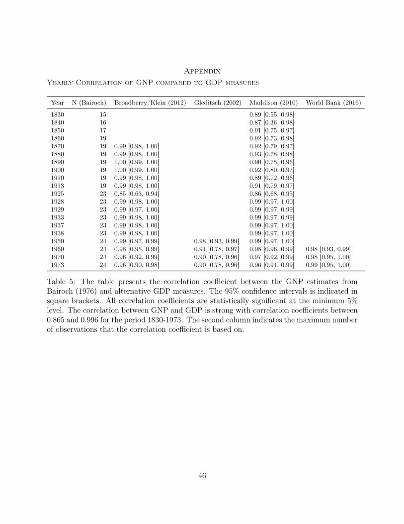
AppendixYearly Correlation of GNP compared to GDP measures
Year N (Bairoch) Broadberry/Klein (2012) Gleditsch (2002) Maddison (2010) World Bank (2016)
1830 15 0.89 [0.55, 0.98]1840 16 0.87 [0.36, 0.98]1850 17 0.91 [0.75, 0.97]1860 19 0.92 [0.73, 0.98]1870 19 0.99 [0.98, 1.00] 0.92 [0.79, 0.97]1880 19 0.99 [0.98, 1.00] 0.93 [0.78, 0.98]1890 19 1.00 [0.99, 1.00] 0.90 [0.75, 0.96]1900 19 1.00 [0.99, 1.00] 0.92 [0.80, 0.97]1910 19 0.99 [0.98, 1.00] 0.89 [0.72, 0.96]1913 19 0.99 [0.98, 1.00] 0.91 [0.79, 0.97]1925 23 0.85 [0.63, 0.94] 0.86 [0.68, 0.95]1928 23 0.99 [0.98, 1.00] 0.99 [0.97, 1.00]1929 23 0.99 [0.97, 1.00] 0.99 [0.97, 0.99]1933 23 0.99 [0.98, 1.00] 0.99 [0.97, 0.99]1937 23 0.99 [0.98, 1.00] 0.99 [0.97, 1.00]1938 23 0.99 [0.98, 1.00] 0.99 [0.97, 1.00]1950 24 0.99 [0.97, 0.99] 0.98 [0.93, 0.99] 0.99 [0.97, 1.00]1960 24 0.98 [0.95, 0.99] 0.91 [0.78, 0.97] 0.98 [0.96, 0.99] 0.98 [0.93, 0.99]1970 24 0.96 [0.92, 0.99] 0.90 [0.78, 0.96] 0.97 [0.92, 0.99] 0.98 [0.95, 1.00]1973 24 0.96 [0.90, 0.98] 0.90 [0.78, 0.96] 0.96 [0.91, 0.99] 0.99 [0.95, 1.00]
Table 5: The table presents the correlation coefficient between the GNP estimates fromBairoch (1976) and alternative GDP measures. The 95% confidence intervals is indicated insquare brackets. All correlation coefficients are statistically significant at the minimum 5%level. The correlation between GNP and GDP is strong with correlation coefficients between0.865 and 0.996 for the period 1830-1973. The second column indicates the maximum numberof observations that the correlation coefficient is based on.
46

Summary Statistics of Observed Variables
Table 6: Summary statistics for components of latent variable models.
Statistic Min Median Mean Max St. Dev. N
GDP Maddison (2010): 1500-2008 1.099 9.647 9.760 16.065 1.950 11,794GDP Gleditsch (2002): 1950-2011 2.944 9.900 9.947 16.395 2.307 8,724GDP World Bank (2016): 1960-2015 16.881 23.405 23.616 30.437 2.427 8,107GDP Broadberry/Klein (2012): 1870-2001 7.114 11.138 11.068 15.574 1.569 2,338GNP Bairoch (1972): 1830-1973 5.298 8.691 8.698 13.063 1.467 415GDP p.c. Maddison (2013): 1500-2000 5.315 7.665 7.762 10.667 1.002 13,068GDP p.c. Gleditsch (2002): 1950-2011 4.889 8.319 8.399 13.357 1.252 8,724GDP p.c. World Bank (2016): 1960-2015 4.749 8.069 8.151 11.886 1.498 7,970GDP p.c. Broadberry/Klein (2012): 1870-2001 6.696 8.390 8.446 10.154 0.793 2,566GNP p.c. Bairoch (1976): 1830-1973 5.136 6.242 6.347 8.159 0.727 369GDP p.c. Broadberry (2015): 1500-1850 6.321 7.012 6.991 8.005 0.474 51Population Maddison (2010): 1500-2010 3.223 8.749 8.872 14.102 1.619 14,138Population Gleditsch (2002): 1950-2011 1.792 8.713 8.455 14.096 2.177 8,724Population World Bank (2016): 1960-2013 8.397 15.390 15.101 21.039 2.230 10,646Population Broadberry/Klein (2012): 1870-2001 0.207 2.288 2.541 5.665 1.219 2,802Population Singer et al. (1972): 1816-2001 2.197 8.761 8.713 14.097 1.801 12,285
The exact measurement of the GDP, per capita GDP, and population variables differs across different sources.See variable description tables for details on the measurement.
47

JAGS Model Codemodel{for(i in 1:n){
# GDP itemsfor(j in 1:5){
xb[i,j] <- b0[j] + b1[j] * x.gdp[i]y[i,j] ~ dnorm(xb[i,j], tau1)y.star[i,j] ~ dnorm(xb[i,j], tau1)
}
# Population itemsfor(j in 6:10){
xb[i,j] <- b0[j] + b1[j] * x.pop[i]y[i,j] ~ dnorm(xb[i,j], tau2)y.star[i,j] ~ dnorm(xb[i,j], tau2)
}
# GDP Per Capita itemsfor(j in 11:16){
xb[i,j] <- b0[j] + b1[j] * x.gdppc[i]y[i,j] ~ dnorm(xb[i,j], tau3)y.star[i,j] ~ dnorm(xb[i,j], tau3)
}
# latent traitsx.gdp[i] <- mu1[country[i], year[i]]x.pop[i] <- mu2[country[i], year[i]]x.gdppc[i] <- log(exp(x.gdp[i]) / exp(x.pop[i]))
}
# priors for the latent traitssigma[1] ~ dunif(0,1)kappa[1] <- pow(sigma[1], -1) # invert to precision
sigma[2] ~ dunif(0,1)kappa[2] <- pow(sigma[2], -1) # invert to precision
for(c in 1:n.country){mu1[c, 1] ~ dnorm(0, 1)mu2[c, 1] ~ dnorm(0, 1)for(t in 2:n.year){ #n.year is number of yearsmu1[c, t] ~ dnorm(mu1[c, t-1], kappa[1])mu2[c, t] ~ dnorm(mu2[c, t-1], kappa[2])
}}
# priors for the model estimatesfor(j in 1:k){b0[j] ~ dnorm(B0[j],4)b1[j] <- 1}
tau1 ~ dgamma(0.001,0.001)tau2 ~ dgamma(0.001,0.001)tau3 ~ dgamma(0.001,0.001)
}
48