Instructions for use

Title Gait posture estimation using wearable acceleration and gyro sensors

Author(s) Takeda, Ryo; Tadano, Shigeru; Natorigawa, Akiko; Todoh, Masahiro; Yoshinari, Satoshi

Citation Journal of Biomechanics, 42(15): 2486-2494

Issue Date 2009-11-13

Doc URL http://hdl.handle.net/2115/42483

Type article (author version)

Additional Information There are other files related to this item in HUSCAP. Check the above URL.

File Information JB42-15_2486-2494.pdf

Hokkaido University Collection of Scholarly and Academic Papers : HUSCAP

- 1 -

Gait Posture Estimation using Wearable Acceleration and

Gyro Sensors

Ryo Takeda a, Shigeru Tadano a*, Akiko Natorigawa a, Masahiro Todoh a

Satoshi Yoshinari b

a Division of Human Mechanical Systems and Design, Graduate School of Engineering,

Hokkaido University, Sapporo, Japan

b Human Engineering Section, Product Technology Department, Hokkaido Industrial

Research Institute, Sapporo, Japan

* Corresponding Author:

Shigeru TADANO, PhD

Professor, Division of Human Mechanical Systems and Design, Graduate School of

Engineering, Hokkaido University

N13 W8, Kita-ku, Sapporo 060-8628, Japan

Tel/Fax: +81-11-706-6405, E-mail: tadano@eng.hokudai.ac.jp

Keywords: Gait Analysis; Acceleration Sensor; Gyro Sensor

Word count: 2982 words (Introduction through Discussion)

Manuscript Type: Original Article

- 2 -

Abstract

A method for gait analysis using wearable acceleration sensors and gyro

sensors is proposed in this work. The volunteers wore sensor units that included a

tri-axis acceleration sensor and three single axis gyro sensors. The angular velocity data

measured by the gyro sensors were used to estimate the translational acceleration in the

gait analysis. The translational acceleration was then subtracted from the acceleration

sensor measurements to obtain the gravitational acceleration, giving the orientation of

the lower limb segments. Segment orientation along with body measurements were used

to obtain the positions of hip, knee, and ankle joints to create stick figure models of the

volunteers. This method can measure the three dimensional positions of joint centers of

the hip, knee, and ankle during movement. Experiments were carried out on the normal

gait of three healthy volunteers. As a result, the flexion-extension (F-E) and the

adduction-abduction (A-A) joint angles of the hips and the flexion-extension (F-E) joint

angles of the knees were calculated and compared with a camera motion capture system.

The correlation coefficients were above 0.88 for the hip F-E, higher than 0.721 for the

hip A-A, better than 0.924 for the knee F-E. A moving stick figure model of each

volunteer was created to visually confirm the walking posture. Further, the knee and

ankle joint trajectories in the horizontal plane showed that the left and right legs were

Response

A-1

- 3 -

bilaterally symmetric.

- 4 -

1. Introduction

Gait analysis is a clinical tool for obtaining quantitive information of the gait of

a person to diagnose walking disabilities. Common methods of gait analysis include

using cameras to track the position of body-mounted reflective markers, from which

information on joint and limb segment motion can be derived. However, such systems

are large, expensive and complex. Therefore, measurements are usually restricted to

indoor laboratories.

An alternative method for measuring human motion is by placing small

acceleration sensors on the body (Morris, 1973). Such inertial sensors allow

measurements to be made outside the laboratory environment (Veltink et al., 1996,

Bouten et al., 1997, Bussmann et al., 1998, Foerster et al., 1999). In contrast to

conventional camera systems, inertial sensor systems do not measure positions.

Therefore, many reports have proposed methods to calculate three dimensional

positions.

A common method to estimate body segment orientation is by integrating

angular velocity data measured by gyro sensors worn on body segments (Tong and

Granat, 1999). However, here small errors in the angular velocity data accumulate with

integration, resulting in errors in the body segment orientation calculations. To reduce

Response

A-1

Response

A-1

- 5 -

the extent of the integration errors, signal filtering based on assumptions of the cyclic

properties of gait has been applied. However this has been restricted to the

measurements of cyclic gait. Further, method is the use of neural networks to predict

joint angles from acceleration and angular velocity data (Findlow et al., 2008). Here

high correlations were reported with the camera analysis, however the creation of such a

prediction system requires much training data for the neural network before accurate

predictions can be made. Other methods have used sophisticated Kalman filters to

eliminate errors included in the sensor data to provide accurate three dimensional

segment calculations (Luinge and Veltink. 2005). In addition, a combination of

acceleration, gyro, and magnetic sensors were used to increase the accuracy (Zhu and

Zhou, 2004, Roetenberg et al., 2007). However, reports showed that there were three

dimensional orientation accuracy errors when compared with the camera analysis even

in static states (Brodie et al., 2008). To avoid such errors, recalibration of the sensors

had to be conducted regularly. Further, magnetic sensors are affected by ferrous

compounds, and careful attention must be given to the magnetic surroundings and even

the storage of the sensors.

Theoretically, it is possible to estimate the orientation of segments by the

gravitational acceleration measured by acceleration sensors. However, in dynamic states

Response

A-1

- 6 -

such as the gait, a translational acceleration component will become included. The

authors (Takeda et al., 2009) have used the cyclic patterns in acceleration data during

gait to create an algorithm to obtain optimal gravitational acceleration patterns. Here, an

optimal three dimensional representation for a person in the base coordinate system was

reported, but there were differences in joint angles established with a camera based

system. In addition, the method was only applicable to cyclic motion such as the gait.

Utilization of signal filters and optimization algorithms for acceleration and

angular velocity data limited measurements to cyclic gait, and the use of magnetic

sensors is not suitable for measurements in home environments. The work reported here

proposes a method for gait analysis using only acceleration and gyro sensors that

measure various kinds of gait in home environments. Here, the angular velocity was

used to calculate the translational acceleration during the gait. The estimated

translational acceleration was then subtracted from the measured acceleration data to

obtain the gravitational acceleration. The gravitational acceleration provided the

orientation angle of the segments and consequently the three dimensional posture of

lower limb segments. To test the method, the gaits of three healthy volunteers were

measured during walking on a flat floor. As a result, the hip flexion-extension (F-E), hip

abduction-adduction (A-A) and knee flexion-extension (F-E) were estimated. The

- 7 -

characteristic three-dimensional walking established by this method could be visualized

in the form of a stick figure model moving in a base coordinate system.

- 8 -

2. Method

2.1 Sensor System

The sensor system used in this investigation consisted of small wearable sensor

units, each containing a data logger and a sensor head. The sensor head has a tri-axial

acceleration sensor (H34C, Hitachi Metals, Ltd.) and three gyro sensors (ENC-03M,

muRata Manufacturing Co., Ltd.), and one sensor unit can measure the acceleration and

the angular velocity along three orthogonal axes simultaneously. The data logger can

record the acceleration and angular velocity data for a maximum of 160 seconds at a

sampling rate of 100Hz. One sensor unit weighs 136 g, including battery (90 g), and the

size is 50mm × 50mm × 15mm for the data logger and 15mm × 15mm × 15mm for the

sensor head. All sensor units were checked on a mechanical turntable to establish the

offset values for acceleration and angular velocity data, in addition to obtaining the

inclination relationships of the measured values. These data were used for the initial

zero offset of the sensors and for converting measured values to acceleration and

angular velocity during the analysis.

- 9 -

2.1 Using acceleration sensors as inclination sensors

Sensor units are placed on the lower limb segments of the volunteers as shown

in Fig. 1. Sensor units are placed on four body segments, on both thighs and both shanks

(RT, LT, RS, and LS). In this report, the length and inclination of each segment was

used to calculate the joint positions of both left and right hips, both knees, and both

ankles (RH, LH, RK, LK, RA, and LA) during walking.

First, a tri-axial acceleration sensor is used as an inclination sensor, as it can

measure the gravitational acceleration, and the output of an acceleration sensor Oi can

be expressed as

),,( zyxigaO iii (1)

Here, ai is the translational acceleration and gi is the gravitational acceleration, both

measured along the i axis of the acceleration sensor. If the acceleration sensor is static

the ai is 0, meaning that the gravitational acceleration is the only output. Therefore, the

angle of inclination for the three axes of an acceleration sensor against the gravitational

acceleration direction can be expressed as

gOcosθ i1

i (2)

and the gravitational acceleration as

222zyx OOOg (3)

- 10 -

2.2 Lower limb posture calculation

The following vectors are used for calculating the hip joint and knee joint

angles.

zyx ,g,gg g g (4)

,a,aa BzByBxBB a a (5)

BzByBx ,O,OO O O BB (6)

BzByBx ,ω,ωω BB ω ω (7)

JBr 0 , 0 , - JBJB r r (8)

The terms used in these equations are detailed in Table 1, and a moving average of 15

data points was used to remove noise in the raw acceleration and angular velocity data.

2.3 Measurements of hip joint angles

The hip joint angle can be calculated with the inclination angle of the thigh

segment, and the acceleration and angular velocity data for the thigh segment, LT and

RT, are used to estimate the segment inclination.

Since gait is a dynamic state, ai in Eq. (1) must be determined before Eq. (2)

can be used to calculate the angles of inclination for the x, y, and z axes of the sensor

- 11 -

unit. A simple model for thigh and shank is shown in Fig. 2(a), here RH, RK, and RA

are the centers of the joints for the hip, knee, and ankle of the right leg, and SRT and SRS

are the centers of the sensor units placed on the thigh and shank respectively. The

calculations for the SRT can be divided into translational motion and rotational motion.

The movement of the hip joint angle is complex, and the thigh and shank was

considered as a double pendulum with the center of the hip joint as the fulcrum. For

simplification, it was assumed that the centripetal and tangential accelerations were

dominant and that there was no translational acceleration, so translational acceleration

becomes 0, and only the rotational motion needs to be calculated. The rotational

acceleration for RH can be expressed as

HTTTHTTHT rωωrω r (9)

with HTr the only acceleration, Eq. 1 is transformed into

THT Org (10)

and now the inclination of the thigh θx, θy, and θz can be calculated by Eq. (2).

In this work, Euler angles are adopted to convert segment inclination angles

into hip joint angles, and the conversions used in Davis et al. (1991) was used. The

Pitch angle will be considered the flexion and extension, the Roll angle the abduction

and adduction, and the Yaw angle the inner and exterior rotation of the hip joint. The

- 12 -

Yaw angle will not be considered in the calculations of this work, and the Pitch and Roll

angles are obtained by the following equations

90xPitch (11)

ycosθsin(Roll)cos(Pitch) (12)

- 13 -

2.4 Measurements of knee joint angles

The acceleration and angular velocity data from the thigh segments, LT and RT,

and the shanks, LS and RS, are used to estimate the knee F-E. The translational

acceleration aT, can be expressed using the following equations

KTKT raa (13)

KTTTKTTKT rωωrω r (14)

Here aK is the acceleration at a joint RK or LK, and the acceleration outputs of SRT or

SLT can be expressed as

gaO TT (15)

If KTr is subtracted from both sides of Eq. (19) it be expanded as

ga g)r(aO KKTHT (16)

Since the ga K measured from SRT (or SLT) and SRS (or SLS) should be the same, the

following equation would hold

KSSKTTK r Or O g a (17)

The method for obtaining knee joint angles is shown in Fig. 2(b1) and 2(b2). Here θ1 is

the angle of inclination of ga K in relation to RT (or LT) segment and θ2 is the angle

of inclination of ga K in relation to RS (or LS) segment. The values of θ1 and θ2 can

be calculated by the following equations

- 14 -

z

x-1 tanKTT

KTT

r O

r O

1 (18)

z

x-1 tanKSS

KSS

r O

r O

2 (19)

Since the knee F-E is equal to the difference between θ2 and θ1, the following holds

2 1 (20)

Though the method shown here is similar to that proposed by Dejnabadi et al.

(2005), the calculations have been simplified by considering the sensor measurements

as the measurements at the center of the link model as shown in Fig.2.

- 15 -

2.5 Creating stick figure model

Stick figure representations of the volunteers were created to be able to

visually confirm the positions of the lower limb segments during walking. The left and

right hip and knee joint angles, and the segment lengths were used to create a relative

coordinate system.

The origin of the relative coordinate system o (0, 0, 0) was at the median point

between the right and left hip joints. The coordinates for RH, LH, RS, LS, RA, and LA

were obtained with the following

),,( 02

0 HHLx,y,zH 　 (21)

T

thighHH L

ed

2

L0

0

x,y,zK 0

0

(22)

T

shankL

0

0

fedKx,y,zA 　 (23)

Here, β is either right or left (R or L), and d, e, and f are rotation matrices.

pitchpitch

pitchpitch

cos0sin

010

sin0cos

d

__

__

(24)

- 16 -

rollroll

rollroll

cossin0

sincos0

001

e

__

__

(25)

cos0sin

010

sin0cos

f (26)

LHH is the distance between the right and left hip joints, Lthigh is the distance between the

hip and knee joints, Lshank is the distance between the knee and ankle joints, and θβ_pitch,

θβ_roll ,and φβ are the pitch, the roll and the F-E angle of the knee.

To convert the position of the joints in the relative coordinate system into the

base coordinate system, the time of heel contact was used. It was reported elsewhere

that a sudden drop in the acceleration data can be used to detect heel contact (Currie et

al., 1992; Auvinet et al., 2002; Mansfield and Lyons, 2003), and this work used the

acceleration at the shank, RS and LS, to determine the time when the leg was set on the

ground. Once the point when the leg is set on the ground is determined, the ankle joint,

RA or LA, is defined as the (X, Y, 0) of the base coordinate system. Since the relative

position of the other joint positions, RK, LK, RH, and LH, are known these positions in

the base coordinate system can be calculated from the ankle joint RA or LA (Fig. 2(c)).

- 17 -

3. Experiment

Three healthy volunteers took part in the experiments and details of the

volunteers are shown in Table 2. For the experiments, four sensor units were placed at

the lower limb (left and right thigh [LT, RT], left and right shank [LS, RS]) of the

volunteers (Fig.3). For comparison, a reference motion analysis system (DIPP-Motion

Pro, Ditect Co., Ltd.) was used to track reflective markers on the volunteers as well. The

volunteers walked for 5 meters on a flat floor inside the laboratory for three trails. The

walking velocity was fixed to a cadence of 88 steps/min using a digital metronome

(TU-80, Roland Corporation). Though the proposed system can measure walking for

longer distances, the measurement was limited to 5m due to the range of the camera

system. Measurements for each volunteer were made to obtain the distances between

each of the lower limb joints.

To prevent sensor attachment errors, measurements of each sensor unit were

made before and after the trials of each volunteer. The measurements of each sensor

were taken in two postures, standing upright and sitting flat with outstretched legs on

the floor. Using the measurements of the two different postures, a calibration of the

three orthogonal axes for the sensor units was conducted. The calibration aligned one

- 18 -

axis to the longitudinal direction of the segment, one axis to the anterior direction, and

one axis to the left lateral direction.

- 19 -

4. Results

Figures 4 and 5 show the results for the measurements of the hip F-E, hip A-A

and knee F-E during gait. The vertical axis represents the angles in degrees and the

horizontal axis the time in seconds. The thick line represents the joint angles measured

for the right leg and the thin line represents the angles of the left leg. The measurements

are of the three volunteers (a), (b), and (c).

A comparison of hip F-E, hip A-A, and knee F-E between this method and the

camera system is possible by looking at Fig. 6 and 7. The vertical axis represents the

angles in degrees and the horizontal axis the percentage of one gait cycle. The joint

angles calculated using this method are shown by the thick lines and the reference

camera system by the thin lines. The phase lag in the peak flexion joint angle, observed

in Fig.7, could be caused by the moving average used to remove noise from the raw

acceleration and angular velocity data. Table 3 shows the RMSE, absolute deviation

(AD) of error, correlation coefficient (CC) and percentage of variance unexplained

(PVU) between the joint angles calculated from this method and that of camera for all

three volunteers.

Figure 8 shows the hip and knee joint trajectories in the horizontal plane. The

vertical and horizontal axes represent the measurements in x and y coordinates

- 20 -

respectively, with (0,0) as the center of the right and left hip joint.

Figure 9 is a stick figure representation of a volunteer using this method and

the reference camera system. Here the abdomen segment for the stick figure is shown

for illustration purposes only. Software developed for this work showed the volunteer’s

gait in the X-Z plane and in the Y-Z plane.

- 21 -

5. Discussion

First, the average of the hip F-E for all the volunteers was: RSME = 8.72 deg,

AD = 6.57 deg, CC = 0.88 and PVU = 20.05%. With the CC and the PVU low, the

results show that this method measures the hip F-E with high consistency to that of the

camera. For the hip A-A the average values were: RSME = 4.96 deg, AD = 3.30 deg,

CC = 0.72 and PVU = 39.29%. The low RSME and AD are caused by the absolute

range of the A-A motions being smaller than to F-E motions of the hip. The low CC and

high PVU may indicate an effect of the internal-external (I-E) rotation during gait

motion. The method here did not consider I-E motion, and including measurements of

this could improve the results, an issue to consider in future work. The average knee

F-E values were: RSME = 6.79 deg, AD = 4.65 deg, CC = 0.92 and PVU = 14.60%. The

knee F-E had higher CC and lower PVU averages than the hip F-E. The CC average of

0.92 for the knee F-E was consistent with the results using wearable sensors provided

by Tong and Granat (1999), and Dejnabadi et al. (2005) where the CC were 0.93 and

0.99 respectively. It may be concluded that the knee F-E can be measured with

significant accuracy using wearable sensors.

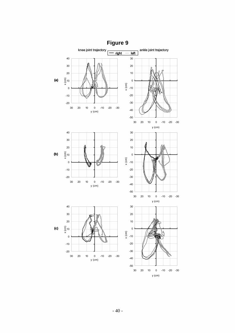
The knee trajectories in Fig. 8 showed that the knee and ankle joint trajectories

were symmetric for both the right and left legs, with the exception of one volunteer (c).

- 22 -

It was not established why the ankle joint trajectories were so different for the right leg,

it is suspected that the sensor sRS could have moved during the trial. This would have

caused errors in the orientation calculations for the right shank.

The method presented here showed a strong correlation with the camera system

data and involved significantly less calculation than reported in previous reports

(Takeda et al., 2009). Further, the method here does not require measurements of the

cyclic gait over long periods of time. One limitation of this work is in the assumption of

constant velocity in the walking direction, and the method introduced here is based on

the assumption that the hip joint movement includes only centripetal and tangential

acceleration. It has been reported that the anterior-posterior acceleration of the trunk

segment increased with walking velocity (Zijlstra and Hof, 2003), and as the current

work conducted experiments at fairly low velocity (88 steps/min), the effect of any

anterior-posterior acceleration may not have been apparent. However, non-constant

motion or gaits at higher velocities may lead to measurement errors and this has to be

controlled for. In addition, errors introduced by the attachment of the sensors is an issue

with any kind of wearable sensor. During movement the attached sensor may move

causing errors in the measurements. This problem can be controlled for by conducting a

predefined motion calibration process before each trial. The work here used the upright

- 23 -

and sitting positions to align the sensor axes in the sagittal plane. Future work will be

needed to develop a more secure method for fixation of the sensors.

With the limitations detailed here, the work here shows that wearable

acceleration and gyro sensors can provide quantitive measurements of human gait

motion with high accuracy as expressed by joint angles, joint trajectories and presented

in stick figures. Future work will be required to develop a method for calculating the

internal-external rotation of the hip joints to provide more accurate results.

- 24 -

Awknowlegement

The authors wish to express thanks to H. Miyagawa of the Laboratory of Biomechanical

Design (Division of Human Mechanical Systems and Design, Hokkaido University), for

support and cooperation in the experiments and computer data analysis of this study.

Conflict of interest’s statement

There are no actual or potential conflicts of interest related to the research reported here.

References

Auvinet, B., Gloria, E., Renault, G., Barrey, E., 2002. Runner’s stride analysis:

comparison of kinematic and kinetic analyses under field conditions. Science &

Sports, 17, 92-94.

Bouten, C.V.C., Koekkoek, K.T.M., Verduin, M., Kodde, R., Janssen, J.D., 1997. A

triaxial accelerometer and portable data processing unit for the assessment of daily

physical activity. IEEE Transactions on Biomedical Engineering, 44, 136-147.

Brodie, M.A., Walmsely, A., Page, W., 2008. The static accuracy and calibration of

inertial measurement units for 3D orientation. Computer Methods in Biomechanics

and Biomedical Engineering, 11, 641-648.

- 25 -

Bussmann, J. B. J., van de Laar, Y. M., Neeleman, M. P., Stam, H. J., 1998. Ambulatory

accelerometry to quantify motor behaviour in patients after failed back surgery: a

validation study. Pain, 74, 153-161.

Currie, G., Rafferty, D., Duncan, G., Bell, F., & Evans, A. L., 1992. Measurement of gait

by accelerometer and walkway: a comparison study. Medical and Biological

Engineering and Computing, 30, 669-670.

Davis, R. B. III, Ounpuu, S., Tyburski, D., Gage, J. R., 1991. A gait analysis data

collection and reduction technique. Human Movement Science, 10, 575-587.

Dejnabadi, H., Jolles, B.M., Aminian, K., 2005. A new approach to accurate

measurement of uniaxial joint angles based on a combination of accelerometers and

gyroscopes. IEEE Transactions on Biomedical Engineering, 52, 1478-1484.

Findlow, A., Goulermas, J.Y., Nester, C., Howard, D., Kenny, L.P.J., 2008. Predicting

lower limb joint kinematics using wearable motion sensors. Gait

Foerster, F., Smeja, M., Fahrenberg, J., 1999. Detection of posture and motion by

accelerometry: a validation study in ambulatory monitoring. Computers in Human

Behavior, 15, 571-583.

Luinge, H. J. and Veltink, P. H., 2005. Measuring orientation of human body segments

using minature gyroscopes and accelerometers. Medical & Biological Engineering &

- 26 -

Computing, 43, 273-282.

Morris, J.R.W., 1973. Accelerometry - A technique for the measurement of human body

movements. Journal of Biomechanics, 6, 729-736.

Mansfield, A., & Lyons, G. M. (2003). The use of accelerometry to detect heel contact

events for use as a sensor in FES assisted walking, Medical Engineering & Physics,

25, 879-885.

Roetenberg, D.; Slycke, P. J.; Veltink, P. H, 2007. Ambulatory position and orientation

tracking fusing magnetic and inertial sensing. IEEE Transactions on Biomedical

Engineering, 54, 883-890.

Takeda, R., Tadano, S., Todoh, M., Morikawa, M., Nakayasu, M., Yoshinari, S., 2009.

Gait analysis using gravitational acceleration measured by wearable sensors. Journal

of Biomechanics, 43, 223-233.

Tong, K. and Granat, M. H., 1999. A practical gait analysis system using gyroscopes.

Medical Engineering and Physics, 21, 87-94.

Veltink, P.H., Bussmann, HansB.J., de Vries, W., Martens, WimL.J., Van Lummel, R.C.,

1996. Detection of static and dynamic activities using uniaxial accelerometers. IEEE

Transactions on Rehabilitation Engineering, 4, 375-385.

Zhu, R. and Zhou, Z., 2004. A real-time articulated human motion tracking using

- 27 -

tri-axis inertial/magnetic sensors package. IEEE Transactions on Neural Systems and

Rehabilitation Engineering, 12, 295-302.

Zijlstra, L. and Hof, A. L., 2003. Assessment of spatio-temporal gait parameters from

trunk accelerations during human walking. Gait and Posture, 18, 1-10.

- 28 -

Figure Legends

Figure 1 Gait model and coordinate systems. The X, Y, Z coordinates represents the base

coordinate system, where the X axis is the walking direction, the Y axis is the left-lateral

direction, and the Z axis is the direction opposite to gravity. The sensors are placed on 4

locations RT, LT, RS and LS.

Figure 2 Measurements for hip and knee joint angles of the right leg. (a) rHT is the

distance from RH to SRT, rKT is the distance from RK to SRT, rKS is the distance from RK

to SRS. (b1) θ1 is the inclination angle of ax-g against RH-RK, θ2 is the inclination

angle of ax-g against RK-RA. (b2) the difference of θ2 and θ1 is equivalent to the knee

joint flexion angle.

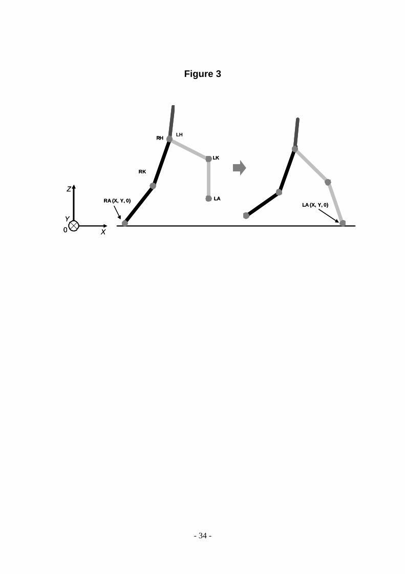
Figure 3 Conversion of relative coordinate joint positions to base coordinate system.

Heel contact is used to determine which foot is set on the ground. The Z coordinate of

the ankle joint set on the ground is considered to be 0.

Figure 4 Sensor attachment locations during experiment. Reflective markers are placed

on the volunteers to track movements using reference camera motion analysis system.

- 29 -

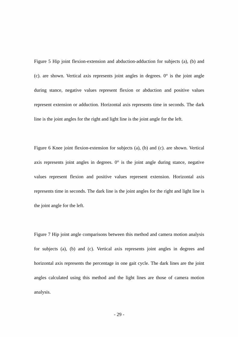
Figure 5 Hip joint flexion-extension and abduction-adduction for subjects (a), (b) and

(c). are shown. Vertical axis represents joint angles in degrees. 0° is the joint angle

during stance, negative values represent flexion or abduction and positive values

represent extension or adduction. Horizontal axis represents time in seconds. The dark

line is the joint angles for the right and light line is the joint angle for the left.

Figure 6 Knee joint flexion-extension for subjects (a), (b) and (c). are shown. Vertical

axis represents joint angles in degrees. 0° is the joint angle during stance, negative

values represent flexion and positive values represent extension. Horizontal axis

represents time in seconds. The dark line is the joint angles for the right and light line is

the joint angle for the left.

Figure 7 Hip joint angle comparisons between this method and camera motion analysis

for subjects (a), (b) and (c). Vertical axis represents joint angles in degrees and

horizontal axis represents the percentage in one gait cycle. The dark lines are the joint

angles calculated using this method and the light lines are those of camera motion

analysis.

- 30 -

Figure 8 Knee joint angle comparisons between this method and camera motion

analysis for subjects (a), (b) and (c). Vertical axis represents joint angles in degrees and

horizontal axis represents the percentage in one gait cycle. The dark lines are the joint

angles calculated using this method and the light lines are those of camera motion

analysis.

Figure 9 Knee and ankle joint trajectories calculated using this method for subjects (a),

(b) and (c). The dark thin line is the trajectory of the left and the light line is that of right

leg. The trajectories are represented in the x-y plane of relative coordinate system o.

Both vertical and horizontal axes are measurements in cm.

Figure 10 Stick figure visualization program. The program shows the stick figure

representations of this method (top) and camera (bottom). This program shows the both

walking in the X-Z base coordinate plane (left) and Y-Z base coordinate plane (right)

simultaneously. The dark heavy line is 0 in the Z coordinate and shown as reference.

- 31 -

Table Legend

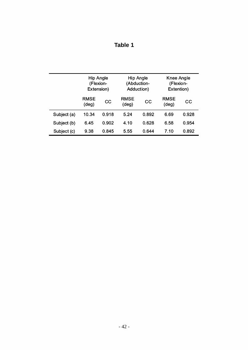
Table 1 The RSME and coefficient correlation of the hip flexion-extension, hip

abduction-adduction and knee flexion-extension. The results are shown separately for

subjects (a), (b) and (c).

- 32 -

Figure 1

Z

X

Y

RH

LH

LK

LA

0

X ,Y, Z : base coordinate systemX : walking direction, Y : lateral direction , Z: opposite direction of gravity

Segment Symbols : RT (right thigh), RS (right shank), LT (left thigh), LS (left shank)

Joint Symbols : RH (right hip), RK (right knee), RA (right ankle), LH (left hip), LK (left knee), LA (left ankle) o (median point of left and right hip)

sensor(sLT)

sLS

sRT

sRS

RK

RA

Walking Direction

o

Z

X

Y

RH

LH

LK

LA

0

X ,Y, Z : base coordinate systemX : walking direction, Y : lateral direction , Z: opposite direction of gravity

Segment Symbols : RT (right thigh), RS (right shank), LT (left thigh), LS (left shank)

Joint Symbols : RH (right hip), RK (right knee), RA (right ankle), LH (left hip), LK (left knee), LA (left ankle) o (median point of left and right hip)

sensor(sLT)

sLS

sRT

sRS

RK

RA

Walking Direction

o

- 33 -

Figure 2

rHT

RK

RA

SRT

XO

Z

Y

rKT

rKSSRS

RH

RA

θ2

θ1

RH

RK

RH

RK

RA

g aK g aK

(a) (b1) (b2)

rHT

RK

RA

SRT

XO

Z

Y

rKT

rKSSRS

RH

RA

θ2

θ1

RH

RK

RH

RK

RA

g aK g aK

(a) (b1) (b2)

- 34 -

Figure 3

Z

X

RHLH

LK

LA

0

RK

RA (X, Y, 0)LA (X, Y, 0)

Y

Z

X

RHLH

LK

LA

0

RK

RA (X, Y, 0)LA (X, Y, 0)

Y

- 35 -

Figure 4

RT(Right Thigh) RT(Right Thigh)

RS(Right Shank) RS(Right Shank)

RT(Right Thigh) RT(Right Thigh)

RS(Right Shank) RS(Right Shank)

- 36 -

Figure 5

-20

0

20

40

60

2 4 6 8 10 120 2 4 6 8 10-20

0

20

2 4 6 8 10 120 2 4 6 8 10

-20

0

20

2 4 6 8 10 120 2 4 6 8 10

-20

0

20

0 2 4 6 8 100 2 4 6 8 10-20

0

20

40

60

0 2 4 6 8 100 2 4 6 8 10

(a)

(b)

(c)

-20

0

20

40

60

2 4 6 8 10 120 2 4 6 8 10

right left

-20

0

20

40

60

-20

0

20

40

60

-20

0

20

40

60

-20

0

20

-20

0

20

-20

0

20

hip

abdu

ctio

n-ad

duct

ion

angl

e (d

egre

e)

hip

flexio

n-ex

tens

ion

angl

e (d

egre

e)hi

p fle

xion-

exte

nsio

nan

gle

(deg

ree)

hip

flexio

n-ex

tens

ion

angl

e (d

egre

e)

hip

abdu

ctio

n-ad

duct

ion

angl

e (d

egre

e)hi

p ab

duct

ion-

addu

ctio

nan

gle

(deg

ree)

time (s) time (s)

-20

0

20

40

60

2 4 6 8 10 120 2 4 6 8 10-20

0

20

40

60

2 4 6 8 10 120 2 4 6 8 10-20

0

20

2 4 6 8 10 120 2 4 6 8 10-20

0

20

2 4 6 8 10 120 2 4 6 8 10

-20

0

20

2 4 6 8 10 120 2 4 6 8 10-20

0

20

2 4 6 8 10 120 2 4 6 8 10

-20

0

20

0 2 4 6 8 100 2 4 6 8 10-20

0

20

0 2 4 6 8 100 2 4 6 8 10-20

0

20

40

60

0 2 4 6 8 100 2 4 6 8 10-20

0

20

40

60

0 2 4 6 8 100 2 4 6 8 10

(a)

(b)

(c)

-20

0

20

40

60

2 4 6 8 10 120 2 4 6 8 10-20

0

20

40

60

2 4 6 8 10 120 2 4 6 8 10

right left

-20

0

20

40

60

-20

0

20

40

60

-20

0

20

40

60

-20

0

20

40

60

-20

0

20

40

60

-20

0

20

40

60

-20

0

20

-20

0

20

-20

0

20

-20

0

20

-20

0

20

-20

0

20

hip

abdu

ctio

n-ad

duct

ion

angl

e (d

egre

e)

hip

flexio

n-ex

tens

ion

angl

e (d

egre

e)hi

p fle

xion-

exte

nsio

nan

gle

(deg

ree)

hip

flexio

n-ex

tens

ion

angl

e (d

egre

e)

hip

abdu

ctio

n-ad

duct

ion

angl

e (d

egre

e)hi

p ab

duct

ion-

addu

ctio

nan

gle

(deg

ree)

time (s) time (s)

- 37 -

Figure 6

0

20

40

60

80

2 4 6 8 10 120 2 4 6 8 10

0

20

40

60

80

2 4 6 8 10 120 2 4 6 8 10

0

20

40

60

80

0 2 4 6 8 100 2 4 6 8 10

knee

flex

ion-

exte

nsio

nan

gle

(deg

ree)

time (s)

(a)

(b)

(c)

knee

flex

ion-

exte

nsio

nan

gle

(deg

ree)

knee

flex

ion-

exte

nsio

nan

gle

(deg

ree)

0

20

40

60

80

0

20

40

60

80

0

20

40

60

80

right left

0

20

40

60

80

2 4 6 8 10 120 2 4 6 8 100

20

40

60

80

2 4 6 8 10 120 2 4 6 8 10

0

20

40

60

80

2 4 6 8 10 120 2 4 6 8 100

20

40

60

80

2 4 6 8 10 120 2 4 6 8 10

0

20

40

60

80

0 2 4 6 8 100 2 4 6 8 10

knee

flex

ion-

exte

nsio

nan

gle

(deg

ree)

time (s)

(a)

(b)

(c)

knee

flex

ion-

exte

nsio

nan

gle

(deg

ree)

knee

flex

ion-

exte

nsio

nan

gle

(deg

ree)

0

20

40

60

80

0

20

40

60

80

0

20

40

60

80

0

20

40

60

80

0

20

40

60

80

0

20

40

60

80

right left

- 38 -

Figure 7

-20

0

20

6.37 7.245 8.120 50 100-60

-40

-20

0

20

6.37 7.245 8.120 50 100

-20

0

20

6.97 7.64 8.310 50 100-60

-40

-20

0

20

6.97 7.64 8.310 50 100

-20

0

20

8.82 9.53 10.240 50 100-60

-40

-20

0

20

8.82 9.53 10.240 50 100gait cycle (%) gait cycle (%)

20

0

-20

-40

-60

20

0

-20

-40

-60

20

0

-20

-40

-60

hip

flexi

on-e

xten

sion

angl

e (d

egre

e)hi

p fle

xion

-ext

ensi

onan

gle

(deg

ree)

hip

flexi

on-e

xten

sion

angl

e (d

egre

e)

20

0

-20

this method camera

hip

abdu

ctio

n-ad

duct

ion

angl

e (d

egre

e)20

0

-20

20

0

-20hip

abdu

ctio

n-ad

duct

ion

angl

e (d

egre

e)hi

p ab

duct

ion-

addu

ctio

nan

gle

(deg

ree)

(a)

(b)

(c)

-20

0

20

6.37 7.245 8.120 50 100-20

0

20

6.37 7.245 8.120 50 100-60

-40

-20

0

20

6.37 7.245 8.120 50 100

-20

0

20

6.97 7.64 8.310 50 100-20

0

20

6.97 7.64 8.310 50 100-60

-40

-20

0

20

6.97 7.64 8.310 50 100

-20

0

20

8.82 9.53 10.240 50 100-20

0

20

8.82 9.53 10.240 50 100-60

-40

-20

0

20

8.82 9.53 10.240 50 100-60

-40

-20

0

20

8.82 9.53 10.240 50 100gait cycle (%) gait cycle (%)

20

0

-20

-40

-60

20

0

-20

-40

-60

20

0

-20

-40

-60

20

0

-20

-40

-60

20

0

-20

-40

-60

20

0

-20

-40

-60

hip

flexi

on-e

xten

sion

angl

e (d

egre

e)hi

p fle

xion

-ext

ensi

onan

gle

(deg

ree)

hip

flexi

on-e

xten

sion

angl

e (d

egre

e)

20

0

-20

20

0

-20

this method camera

hip

abdu

ctio

n-ad

duct

ion

angl

e (d

egre

e)20

0

-20

20

0

-20

20

0

-20

20

0

-20hip

abdu

ctio

n-ad

duct

ion

angl

e (d

egre

e)hi

p ab

duct

ion-

addu

ctio

nan

gle

(deg

ree)

(a)

(b)

(c)

- 39 -

Figure 8

0

20

40

60

80

6.37 7.245 8.120 50 100

0

20

40

60

80

6.97 7.64 8.310 50 100

0

20

40

60

80

8.82 9.53 10.240 50 100

this method camera

gait cycle (%)

80

60

40

20

0

80

60

40

20

0

80

60

40

20

0

knee

flex

ion-

exte

nsio

nan

gle

(deg

ree)

knee

flex

ion-

exte

nsio

nan

gle

(deg

ree)

knee

flex

ion-

exte

nsio

nan

gle

(deg

ree)

(a)

(b)

(c)

0

20

40

60

80

6.37 7.245 8.120 50 100

0

20

40

60

80

6.97 7.64 8.310 50 100

0

20

40

60

80

8.82 9.53 10.240 50 1000

20

40

60

80

8.82 9.53 10.240 50 100

this method camera

gait cycle (%)

80

60

40

20

0

80

60

40

20

0

80

60

40

20

0

80

60

40

20

0

80

60

40

20

0

80

60

40

20

0

knee

flex

ion-

exte

nsio

nan

gle

(deg

ree)

knee

flex

ion-

exte

nsio

nan

gle

(deg

ree)

knee

flex

ion-

exte

nsio

nan

gle

(deg

ree)

(a)

(b)

(c)

- 40 -

Figure 9

-50

-40

-30

-20

-10

0

10

20

30

-30-20-100102030

y (cm)x

(cm

)

-50

-40

-30

-20

-10

0

10

20

30

-30-20-100102030

y (cm)

x (c

m)

-50

-40

-30

-20

-10

0

10

20

30

-30-20-100102030

y (cm)

x (c

m)

-20

-10

0

10

20

30

40

-30-20-100102030y (cm)

x (c

m)

-20

-10

0

10

20

30

40

-30-20-100102030y (cm)

x (c

m)

-20

-10

0

10

20

30

40

-30-20-100102030y (cm)

x (c

m)

(a)

(c)

(b)

ankle joint trajectoryknee joint trajectoryright left

-50

-40

-30

-20

-10

0

10

20

30

-30-20-100102030

y (cm)x

(cm

)

-50

-40

-30

-20

-10

0

10

20

30

-30-20-100102030

y (cm)

x (c

m)

-50

-40

-30

-20

-10

0

10

20

30

-30-20-100102030

y (cm)

x (c

m)

-20

-10

0

10

20

30

40

-30-20-100102030y (cm)

x (c

m)

-20

-10

0

10

20

30

40

-30-20-100102030y (cm)

x (c

m)

-20

-10

0

10

20

30

40

-30-20-100102030y (cm)

x (c

m)

(a)

(c)

(b)

ankle joint trajectoryknee joint trajectoryright leftright left

- 41 -

Figure 10

This Method

Camera

This Method

Camera

- 42 -

Table 1

0.8927.100.6445.550.8459.38Subject (c)

0.9546.580.6284.100.9026.45Subject (b)

0.9286.690.8925.240.91810.34Subject (a)

CCRMSE(deg)CCRMSE

(deg)CCRMSE(deg)

Knee Angle(Flexion-

Extention)

Hip Angle (Abduction-Adduction)

Hip Angle (Flexion-

Extension)

0.8927.100.6445.550.8459.38Subject (c)

0.9546.580.6284.100.9026.45Subject (b)

0.9286.690.8925.240.91810.34Subject (a)

CCRMSE(deg)CCRMSE

(deg)CCRMSE(deg)

Knee Angle(Flexion-

Extention)

Hip Angle (Abduction-Adduction)

Hip Angle (Flexion-

Extension)