Future permafrost conditions along environmental gradients ... · on the future ground thermal...
17
The Cryosphere, 9, 719–735, 2015 www.the-cryosphere.net/9/719/2015/ doi:10.5194/tc-9-719-2015 © Author(s) 2015. CC Attribution 3.0 License. Future permafrost conditions along environmental gradients in Zackenberg, Greenland S. Westermann 1,2 , B. Elberling 1 , S. Højlund Pedersen 3 , M. Stendel 4 , B. U. Hansen 1 , and G. E. Liston 5 1 Center for Permafrost (CENPERM), Department of Geosciences and Natural Resource Management, University of Copenhagen, Øster Voldgade 10, 1350 Copenhagen K., Denmark 2 Department of Geosciences, University of Oslo, P.O. Box 1047, Blindern, 0316 Oslo, Norway 3 Department of Bioscience – Arctic Research Centre, Aarhus University, Frederiksborgvej 399, 4000 Roskilde, Denmark 4 Danish Climate Centre – Danish Meteorological Institute, Lyngbyvej 100, 2100 Copenhagen, Denmark 5 Cooperative Institute for Research in the Atmosphere, Colorado State University, 1375 Campus Delivery, Fort Collins, CO 80523-1375, USA Correspondence to: B. Elberling ([email protected]) Received: 14 May 2014 – Published in The Cryosphere Discuss.: 16 July 2014 Revised: 25 March 2015 – Accepted: 26 March 2015 – Published: 17 April 2015 Abstract. The future development of ground temperatures in permafrost areas is determined by a number of factors vary- ing on different spatial and temporal scales. For sound pro- jections of impacts of permafrost thaw, scaling procedures are of paramount importance. We present numerical simula- tions of present and future ground temperatures at 10 m res- olution for a 4 km long transect across the lower Zackenberg valley in northeast Greenland. The results are based on step- wise downscaling of future projections derived from general circulation model using observational data, snow redistribu- tion modeling, remote sensing data and a ground thermal model. A comparison to in situ measurements of thaw depths at two CALM sites and near-surface ground temperatures at 17 sites suggests agreement within 0.10 m for the maxi- mum thaw depth and 1 ◦ C for annual average ground tem- perature. Until 2100, modeled ground temperatures at 10 m depth warm by about 5 ◦ C and the active layer thickness in- creases by about 30 %, in conjunction with a warming of av- erage near-surface summer soil temperatures by 2 ◦ C. While ground temperatures at 10 m depth remain below 0 ◦ C until 2100 in all model grid cells, positive annual average temper- atures are modeled at 1 m depth for a few years and grid cells at the end of this century. The ensemble of all 10m model grid cells highlights the significant spatial variability of the ground thermal regime which is not accessible in traditional coarse-scale modeling approaches. 1 Introduction The stability and degradation of permafrost areas are exten- sively discussed regarding future climate changes as poten- tially important source of greenhouse gases (Schuur et al., 2008, 2009; Elberling et al., 2010, 2013), infrastructure sta- bility (Wang et al., 2003, 2006) and farming potential (Mick and Johnson, 1954; Merzlaya et al., 2008). Depending on the emission scenario, future projections based on coarse-scale general circulation models (GCMs) suggest a loss of 30 to 70 % of the current permafrost extent by 2100, in conjunction with a significant deepening of the active layer in the remain- ing areas (Lawrence et al., 2012). However, such projections are based on the modeled evolution of coarse-scale grid cells which may not represent significantly smaller variability of environmental factors governing the thermal regime typical for many permafrost landscapes. Hence, a detailed impact as- sessment of the thermal regime remains problematic, which precludes sound projections of future greenhouse gas emis- sions from permafrost areas. Regional climate models (RCMs) facilitate downscaling of GCM output to scales of several kilometers so that, for example, regional precipitation patterns and topography- induced temperature gradients are much better reproduced. Based on RCM output, projections of the future ground thermal regime have been performed for a number of per- mafrost regions, e.g., northeast Siberia (50 km resolution, Published by Copernicus Publications on behalf of the European Geosciences Union.
Transcript of Future permafrost conditions along environmental gradients ... · on the future ground thermal...

The Cryosphere, 9, 719–735, 2015
www.the-cryosphere.net/9/719/2015/
doi:10.5194/tc-9-719-2015
© Author(s) 2015. CC Attribution 3.0 License.
Future permafrost conditions along environmental gradients
in Zackenberg, Greenland
S. Westermann1,2, B. Elberling1, S. Højlund Pedersen3, M. Stendel4, B. U. Hansen1, and G. E. Liston5
1Center for Permafrost (CENPERM), Department of Geosciences and Natural Resource Management,
University of Copenhagen, Øster Voldgade 10, 1350 Copenhagen K., Denmark2Department of Geosciences, University of Oslo, P.O. Box 1047, Blindern, 0316 Oslo, Norway3Department of Bioscience – Arctic Research Centre, Aarhus University, Frederiksborgvej 399, 4000 Roskilde, Denmark4Danish Climate Centre – Danish Meteorological Institute, Lyngbyvej 100, 2100 Copenhagen, Denmark5Cooperative Institute for Research in the Atmosphere, Colorado State University, 1375 Campus Delivery, Fort Collins,
CO 80523-1375, USA
Correspondence to: B. Elberling ([email protected])
Received: 14 May 2014 – Published in The Cryosphere Discuss.: 16 July 2014
Revised: 25 March 2015 – Accepted: 26 March 2015 – Published: 17 April 2015
Abstract. The future development of ground temperatures in
permafrost areas is determined by a number of factors vary-
ing on different spatial and temporal scales. For sound pro-
jections of impacts of permafrost thaw, scaling procedures
are of paramount importance. We present numerical simula-
tions of present and future ground temperatures at 10 m res-
olution for a 4 km long transect across the lower Zackenberg
valley in northeast Greenland. The results are based on step-
wise downscaling of future projections derived from general
circulation model using observational data, snow redistribu-
tion modeling, remote sensing data and a ground thermal
model. A comparison to in situ measurements of thaw depths
at two CALM sites and near-surface ground temperatures
at 17 sites suggests agreement within 0.10 m for the maxi-
mum thaw depth and 1 ◦C for annual average ground tem-
perature. Until 2100, modeled ground temperatures at 10 m
depth warm by about 5 ◦C and the active layer thickness in-
creases by about 30 %, in conjunction with a warming of av-
erage near-surface summer soil temperatures by 2 ◦C. While
ground temperatures at 10 m depth remain below 0 ◦C until
2100 in all model grid cells, positive annual average temper-
atures are modeled at 1 m depth for a few years and grid cells
at the end of this century. The ensemble of all 10 m model
grid cells highlights the significant spatial variability of the
ground thermal regime which is not accessible in traditional
coarse-scale modeling approaches.
1 Introduction
The stability and degradation of permafrost areas are exten-
sively discussed regarding future climate changes as poten-
tially important source of greenhouse gases (Schuur et al.,
2008, 2009; Elberling et al., 2010, 2013), infrastructure sta-
bility (Wang et al., 2003, 2006) and farming potential (Mick
and Johnson, 1954; Merzlaya et al., 2008). Depending on the
emission scenario, future projections based on coarse-scale
general circulation models (GCMs) suggest a loss of 30 to
70 % of the current permafrost extent by 2100, in conjunction
with a significant deepening of the active layer in the remain-
ing areas (Lawrence et al., 2012). However, such projections
are based on the modeled evolution of coarse-scale grid cells
which may not represent significantly smaller variability of
environmental factors governing the thermal regime typical
for many permafrost landscapes. Hence, a detailed impact as-
sessment of the thermal regime remains problematic, which
precludes sound projections of future greenhouse gas emis-
sions from permafrost areas.
Regional climate models (RCMs) facilitate downscaling
of GCM output to scales of several kilometers so that,
for example, regional precipitation patterns and topography-
induced temperature gradients are much better reproduced.
Based on RCM output, projections of the future ground
thermal regime have been performed for a number of per-
mafrost regions, e.g., northeast Siberia (50 km resolution,
Published by Copernicus Publications on behalf of the European Geosciences Union.

720 S. Westermann et al.: Permafrost in northeast Greenland
Stendel et al., 2007), Greenland (25 km resolution, Daanen
et al., 2011) and Alaska (2 km resolution, Jafarov et al.,
2012). While this constitutes a major improvement, many
processes governing the ground thermal regime vary strongly
at even smaller spatial scales so that the connection between
model results and ground observations is questionable. In
high-Arctic and mountain permafrost areas exposed to strong
winds, redistribution of blowing snow can create a pattern of
strongly different snow depths on distances of a few meters.
Since snow is an effective insulator between ground and at-
mosphere (Goodrich, 1982), a distribution of ground temper-
atures with a range between average maximum and minimum
temperatures of 5 ◦C and more is created (e.g., Gisnås et al.,
2014), which is of a similar order of magnitude to the pro-
jected increase of near-surface air temperatures in many po-
lar areas. Consequently, the susceptibility to climate change
can display a dramatic variability on local scales and per-
mafrost degradation can occur significantly earlier in parts of
a landscape than suggested by coarse-scale modeling. Fur-
thermore, the thermal properties and cryostratigraphy of the
ground can be highly variable as a result of geomorphol-
ogy, vegetation and hydrological pathways, with profound
implications for the thermal inertia and thus the dynamics
of permafrost degradation. In a modeling study for south-
ern Norway, Westermann et al. (2013) highlight that near-
surface permafrost in bedrock areas disappears within a few
years after the climatic forcing crosses the thawing threshold,
while near-surface permafrost is conserved for more than 2
decades in areas with high organic and ground ice contents
and/or a dry, insulating surface layer. In addition, the soil
carbon content in Arctic landscapes is unevenly distributed
(Hugelius et al., 2013), and greenhouse gas emissions from
localized carbon-rich hotspots can contribute a significant
part to the landscape signal (e.g., Walter et al., 2006; Mas-
tepanov et al., 2008). Therefore, both the carbon stocks and
the physical processes governing permafrost evolution must
be understood at the appropriate spatial scales to facilitate
improved predictions of the permafrost–carbon feedback.
In recent years, modeling schemes capable of comput-
ing the ground thermal regime at significantly higher spa-
tial resolutions of 10 to 30 m have been developed and ap-
plied in complex permafrost landscapes (e.g., Zhang, 2013;
Zhang et al., 2012, 2013; Fiddes and Gruber, 2012, 2014;
Fiddes et al., 2015). These approaches can capture small-
scale differences in altitude, aspect and exposition, as well
as in surface and subsurface properties, but the redistribution
of snow through wind drift is only included in a simplified
way through precipitation correction factors (Fiddes et al.,
2015; Zhang et al., 2012). On the other hand, dedicated snow
redistribution models of various levels of complexity exist
(e.g., Winstral et al., 2002; Lehning et al., 2006) with which
the pattern and evolution of snow depths can be simulated.
In this study we make use of such an approach, the deter-
ministic snow modeling system MicroMet/SnowModel (Lis-
ton and Elder, 2006a, b), to achieve high-resolution simula-
tions of the ground thermal regime at the Zackenberg per-
mafrost observatory in northeast Greenland (Meltofte et al.,
2008) until 2100. MicroMet/SnowModel is employed as part
of a sequential downscaling procedure, including the RCM
HIRHAM5 (Christensen et al., 1996) and the ground thermal
model CryoGrid 2 (Westermann et al., 2013). With a spatial
resolution of 10 m, the effect of snow distribution patterns
and different subsurface and surface properties on ground
temperatures can be accounted for. The study aims to fill the
gap between the coarse- and the point-scale modeling studies
on the future ground thermal regime which are available for
the Zackenberg valley so far. The 25 km scale, Greenland-
wide assessment of Daanen et al. (2011) puts Zackenberg
in the zone of “high thaw potential” until the end century,
with modeled ground temperatures of −5 to −2.5 ◦C and an
active layer thickness of 0.5 to 0.75 m for the period 2065–
2075. However, the detailed point-scale study by Hollesen
et al. (2011) suggests a future active layer thickness of 0.8 to
1.05 m for a site with average soil moisture conditions which
are not representative of many other sites found in the Za-
ckenberg valley, such as the wetlands. Extending this ear-
lier work, we present simulations for a 4 km transect cutting
across typical vegetation zones in the lower parts of Zack-
enberg valley which allow estimating the range of ground
thermal conditions that could be encountered until the end of
the century.
2 The Zackenberg site
Zackenberg is located in northeast Greenland at 74◦30′ N,
20◦30′W (Fig. 1). Zackenberg valley is a wide lowland val-
ley dominated by Quaternary non-calcareous sediments with
significant periglacial activity and continuous permafrost
(Elberling et al., 2004, 2008), with a mean annual air temper-
ature of −9.5 ◦C (1996–2007) according to Elberling et al.
(2010). Maximum active layer thickness varies from 40 cm
to more than 2 m and has increased significantly by 0.8 cm
to 1.5 cm per year between 1996 and 2012 (Elberling et al.,
2013), which has been determined at two sites (denoted Zero-
Calm 1 and 2, Fig. 1) of the Circumpolar Active Layer Mon-
itoring (CALM) program (Brown et al., 2000).
From the hilltops towards the depressions, an increase in
soil water content is seen from dry to wet conditions at the
foot of the slopes due to snowmelt water being released dur-
ing large parts of the summer. Roughly one-third of the low-
land area in Zackenberg is poorly drained. Given the low
summer precipitation, water availability during the growing
season is mainly controlled by the location of large snow
patches melting during the growing season, resulting in the
distinct vegetation zonation around these.
The topography, landscape forms and wind direction are
the main factors controlling both water drainage and snow
distribution. These patterns are found on both a landscape
scale and a small scale (100–200 m) and can therefore be il-
The Cryosphere, 9, 719–735, 2015 www.the-cryosphere.net/9/719/2015/
S. Westermann et al.: Permafrost in northeast Greenland 721
Figure 1. Left: location of the Zackenberg site and ZERO-line in Greenland. Right: NDVI image (derived from a multi-spectral Quickbird
2 image from 7 July 2011) of the modeled part of ZERO-line, with the CALM sites ZeroCalm (ZC) 1 and 2 and the locations of in situ
measurements of ground temperatures Tground at different depths, as employed in Sect. 4.1. Two additional in situ measurements of ground
temperatures at shallow depths are located approx. 0.5 km NE and SW of the displayed scene. Coordinates are in UTM zone 27; note that
ZERO-line continues further NE to the top of Aucellabjerg.
lustrated conceptually as a transect across typical landscape
forms in the valley from hilltops to depressions. The top of
the hills are windblown and exposed throughout the year with
little or no accumulation of snow. From the hilltops towards
the depressions there is an increase in soil water content from
dry conditions (even arid conditions and salt accumulation at
the soil surface) at the hilltops to wet conditions in the bottom
of the depression. The dominant wind pattern during winter
leaves large snow patches on the south-facing slopes ensur-
ing high surface and soil water contents during a large part
of the growing season.
Bay (1998) described and classified the plant communi-
ties in the central part of the Zackenberg valley and mapped
their distribution. The vegetation zones range from fens in the
depressions to fell-fields and boulder areas towards the hill
tops. East of the river Zackenbergelven the lowland is domi-
nated by Cassiope tetragona heaths mixed with Salix arctica
snow beds, grasslands and fens; the latter occurring in the
wet, low-lying depressions, often surrounded by grassland.
On the transition from the lowland to the slopes of Aucellab-
jerg (50–100 m a.s.l.), the vegetation is dominated by grass-
land. Between 150 and 300 m a.s.l., open heaths of mountain
avens, Dryas sp., dominate and gradually the vegetation be-
comes more open with increasing altitude towards the fell-
fields with a sparse plant cover of Salix arctica and Dryas sp.
Grassland, rich in vascular plant species and mosses, occurs
along the wet stripes from the snow patches in the highland
(250–600 m a.s.l.).
For monitoring purposes, an 8km transect cutting across
the main ecological zones of the Zackenberg valley from
sea level to 1040 m a.s.l. at the summit of Aucellabjerg has
been established, which is considered representative of the
Zackenberg valley (Fredskild and Mogensen, 1997; Meltofte
et al., 2008). Along this so-called ZERO (“Zackenberg eco-
logical research operations”) line (Fig. 1), changes in species
composition and distribution of plant communities are in-
vestigated regularly. In this study, we focus on lower 4 km
of ZERO-line from the coast to an elevation of 200 m a.s.l.,
which is characterized by a strong variability as exemplified
by the normalized difference vegetation index (NDVI) values
(Fig. 1).
3 Modeling tools
In order to determine the spatial variability of ground tem-
peratures in the Zackenberg valley, simulations from 1960 to
2100 are performed for grid cells of 10 m resolution for the
lower 4 km of ZERO-line (in total 437 grid cells). In addition,
the 100m× 100m large CALM sites ZeroCalm 1 and 2 are
simulated (Fig. 1, in total 200 grid cells). To compile forcing
data sets at such high resolution, a multi-step downscaling
procedure is employed which is schematically depicted in
Fig. 2. It is designed to account for the spatial variability of
snow depths, differences in summer surface temperature (due
to, e.g., different evapotranspiration rates caused by surface
soil moisture and land cover) and spatially variable ground
www.the-cryosphere.net/9/719/2015/ The Cryosphere, 9, 719–735, 2015

722 S. Westermann et al.: Permafrost in northeast Greenland
Figure 2. Schematic workflow of the modeling scheme depicting
field data (green), remote sensing data (red), models (blue) and the
principal forcing data (yellow) for the thermal model CryoGrid 2,
delivering spatially resolved fields of ground temperatures. See text.
thermal properties and water/ice contents. Differences in in-
solation due to exposition and aspect are not accounted for,
which is acceptable for the gentle topography (average slope
2.8◦) in the modeled part of ZERO-line. The different parts
of the scheme and their interplay are described as follows.
3.1 The permafrost model CryoGrid 2
CryoGrid 2 is a one-dimensional, physically based thermal
subsurface model driven by time series of near-surface air
temperature and snow depth and has been recently employed
to assess the evolution of permafrost extent and temperatures
in southern Norway (Westermann et al., 2013). The physical
basis and operational details of CryoGrid 2 are documented
in Westermann et al. (2013), and only a brief overview over
the model properties is given here. CryoGrid 2 numerically
solves Fourier’s law of conductive heat transfer in the ground
to determine the evolution of ground temperature T [K] over
time t ,
ceff(z,T )∂T
∂t−
∂
∂z
(k(z,T )
∂T
∂z
)= 0, (1)
with the thermal conductivity k [Wm−1 K−1] being a func-
tion of the volumetric fractions and thermal conductivities of
the constituents water, ice, air, mineral and organic (West-
ermann et al., 2013) following the formulation of Cosenza
et al. (2003). For the thermal conductivity of the mineral frac-
tion of the soil, we assume 3.0 Wm−1 K−1, which is a typ-
ical value for sedimentary and metamorphic rock with low
quartz content (Clauser and Huenges, 1995), as dominant
in most parts of the Zackenberg valley (Koch and Haller,
1965). For the organic soil fraction, the standard value of
0.25 Wm−1 K−1 (e.g., Côté and Konrad, 2005) for peat is
employed.
The latent heat from freezing soil water or melting ice
is accounted for in terms of an effective heat capacity ceff
[Jm−3 K−1], which increases strongly in the temperature
range in which latent heat effects occur. This curve is de-
termined by the soil freezing characteristic, i.e., the function
linking the soil water content to temperature, which is re-
lated to the hydraulic properties of the soil in CryoGrid 2
(Dall’Amico et al., 2011) for three soil classes: sand, silt and
clay. To account for the buildup and disappearance of the
snow cover, the position of the upper boundary is allowed to
change dynamically by adding or removing grid cells. Move-
ment of soil water is not accounted for so that the sum of the
soil water and ice contents are constant in CryoGrid 2. For
spatially distributed modeling, the target domain is decom-
posed in independent grid cells, each featuring a set of model
parameters.
3.1.1 Model initialization
The initial temperature profile for each grid cell is obtained
by a multi-step initialization procedure which allows us to
approximate steady-state conditions in equilibrium with the
climate forcing for the first model decade (September 1958–
August 1968) in a computationally efficient way. The method
which is described in more detail in Westermann et al. (2013)
accounts for the insulating effect of the seasonal snow cover
as well as the thermal offset (Osterkamp and Romanovsky,
1999).
3.1.2 Driving data sets
As driving data sets for CryoGrid 2 we use gridded data sets
of daily average air temperature and snow depth obtained
from a downscaling scheme and a snow redistribution model
(Sects. 3.3, 3.4). To account for differences in surface soil
moisture between grid cells, which give rise to spatially dif-
ferent surface temperatures, we employ the empirical con-
cept of n factors which relate average air temperature Tair to
surface temperature Ts by Ts = nt Tair:
Ts =
{Tair for Tair ≤ 0 ◦C
nt Tair for Tair > 0 ◦C.(2)
This rough treatment of summer surface temperatures (which
has been applied in previous modeling studies, e.g., Hipp
et al., 2012) is focused on seasonal averages and can not re-
produce surface temperatures on shorter timescales, e.g., the
daily cycle. As a result, a comparison of temperatures in
upper soil layers is less meaningful than for deeper layers,
which are only influenced by seasonal or even multi-annual
average temperatures. However, the n factor-based approach
precludes the need to compute the surface energy balance
and allows employing measured historic time series of air
temperatures (such as the one from Daneborg, Sect. 3.4) for
ground thermal modeling.
The Cryosphere, 9, 719–735, 2015 www.the-cryosphere.net/9/719/2015/

S. Westermann et al.: Permafrost in northeast Greenland 723
Figure 3. Summer nt factor vs. NDVI based on in situ measure-
ments from Zackenberg and Kobbefjord in Greenland and from
northern Alaska (Klene et al., 2001; Walker et al., 2003). The black
line represents the fit following Eq. (3), R2 = 0.97.
The summertime n factor nt is computed according to the
NDVI of each grid cell (at the maximum of the growing sea-
son) using
nt = 2.42NDVI2− 3.01NDVI+ 1.54. (3)
The relationship is compiled with nt as the ratio of degree-
day sums at the soil surface to those in the air over the sum-
mer season at both Zackenberg (74.5◦ N) and Kobbefjord
(65.6◦ N), close to Nuuk in western Greenland. Figure 3 also
shows a strong correlation between nt values (Klene et al.,
2001) and NDVI values (Walker et al., 2003) from the Ku-
paruk River basin, Alaska, USA, with an R2 value of 0.97 for
the combined data set. Summer nt factors above 1 indicate
that the soil-surface temperatures are warmer than air tem-
peratures; this mostly occurs on nearly barren mineral soils.
The minimum nt values of approx. 0.65 are found in moist
fen areas, indicating a strong cooling effect during the sum-
mer on the mineral soils of these sites.
For each 10 m model grid cell, an NDVI value was de-
termined from a 2.5 m multi-spectral Quickbird 2 image of
the Zackenberg area acquired around noon local time on 7
July 2011 (Fig. 1). Whereas the acquisition date is close to
the annual maximum NDVI values, it represents a single
point in the time, and there is strong seasonal and interan-
nual variability in plant growth and consequent evolution of
NDVI values (Tamstorf et al., 2007). While this error source
is hard to quantify, the general agreement in the coverage of
the different vegetation classes (see next section) with field
observations suggests that the satellite image is an adequate
basis to capture the pattern of surface soil moisture and sum-
mer surface temperatures along ZERO-line.
3.1.3 Ground properties
Based on a NDVI-classification, six ecosystems were identi-
fied in Zackenberg valley (Bay, 1998; Tamstorf et al., 2007;
Ellebjerg et al., 2008). Areas with NVDI < 0.2 are domi-
nated by fell-field with a sparse vegetation. In the high moun-
tains such areas are found on solifluction soils, patterned
ground and rocky ravines. Dryas heath dominates areas with
NDVI between 0.2 and 0.3. Fell-field and Dryas heath are
both situated at exposed plateaus, where snow often blows
off during the winter months causing thinner snow cover.
Here, plant species experience an early snowmelt and hence
an early start of the growing season. Cassiope heath (NDVI
between 0.3 and 0.4) depends on a protective snow cover dur-
ing winter and occurs mainly in the lowland on gentle slopes
facing south and leeward from the northerly winds which
dominate the winter period (Hansen et al., 2008). Salix snow
beds feature NDVI values between 0.4 and 0.5. This ecosys-
tem, which is unique to eastern Greenland, occurs mostly on
sloping terrain, often below the Cassiope heath belt on the
slopes, where the snow cover is long lasting so that the soil
moisture in the Salix snow-bed areas are higher. In the wet-
land areas with NDVI higher than 0.5, grassland and fen ar-
eas are distinguished. Grassland occurs mostly on slightly
sloping terrain with an adequate supply of water early in the
season, while the soil water regime can change from wet to
moist later in the season. The fen areas occur on flat terrain
in the lowland, where the soil is permanently water-saturated
throughout the growing season. In August 2013, a classifica-
tion of ecosystem classes according to the dominating plant
species and qualitative surface moisture conditions was con-
ducted along the modeled part of ZERO-line at spatial reso-
lution of 10 m, which resulted in 5 % fell, 20 % Dryas, 35 %
Cassiope, 15 % Salix snow bed and 25 % wetland (fen and
grassland areas were not distinguished).
Using satellite-derived NDVI values (see previous sec-
tion), these ecosystem fractions could be well reproduced
for fell (9 %), Dryas (22 %) and Cassiope (39 %), while a
strong discrepancy was encountered for the Salix and wet-
land classes. Therefore, Salix snow bed was merged with
wetland, yielding a wetland fraction of 30 %. The “true”
Salix class is hereby split between Cassiope and wetland,
which is reflected in the strong concentration of grid cells
with NDVI values around 0.4. This suggests a significant
overlap of the NDVI values from the different classes in this
region for the particular satellite acquisition date, so that the
classes can not be separated by their NDVI value. While the
NDVI-derived ecosystem classification constitutes a poten-
tially important source of uncertainty in the modeling chain,
it provides the possibility to use satellite images and thus ap-
ply the classification procedure for larger regions, e.g., the
entire Zackenberg valley, at high spatial resolutions, which
can hardly be achieved by manual mapping.
For the remaining four classes fell, Dryas, Cassiope and
wetland, typical soil stratigraphies were assigned based on
www.the-cryosphere.net/9/719/2015/ The Cryosphere, 9, 719–735, 2015

724 S. Westermann et al.: Permafrost in northeast Greenland
Table 1. Sediment stratigraphies in CryoGrid 2 with volumetric
fractions of the soil constituents and soil type for each layer given.
Depth (m) Water/ice Mineral Organic Air Type
Fell
0–3 0.05 0.6 0.0 0.35 sand
3–10 0.4 0.6 0.0 0.0 sand
> 10 0.03 0.97 0.0 0.0 sand
Dryas
0–1 0.15 0.55 0.0 0.3 sand
1–10 0.4 0.6 0.0 0.0 sand
> 10 0.03 0.97 0.0 0.0 sand
Cassiope heath
0–0.8 0.25 0.55 0.0 0.2 sand
0.8–10 0.4 0.6 0.0 0.0 sand
> 10 0.03 0.97 0.0 0.0 sand
Wetland
0–0.6 0.5 0.45 0.05 0.0 silt
0.6–10 0.4 0.6 0.0 0.0 silt
> 10 0.03 0.97 0.0 0.0 sand
and guided by in situ measurements in soil samples (Ta-
ble 1). The stratigraphies are designed to represent the char-
acteristics of the different ecosystem classes at least in a
semi-quantitative way: from fell to wetland, the water con-
tents in the active layer increase from dry to saturated con-
ditions, while the soil texture changes from coarse to more
fine-grained in conjunction with increasing porosity. The ab-
solute values are derived from soil samples taken at depths
between 0 and 0.5 m in the different classes mainly in July
2006 and 2007. For wetland and Cassiope, the average of all
values yielded volumetric water contents of 0.52 and 0.28,
respectively. Furthermore, transient simulations of the one-
dimensional water balance and ground thermal regime with
the COUP model suggest average soil water contents be-
tween 0.2 and 0.3 for the active layer at a Cassiope site
(Hollesen et al., 2011). For the Dryas and fell classes, large
changes in soil moisture were encountered after rain falls
which made the values strongly dependent on the timing of
the sampling. The volumetric organic material contents are
low in all classes (5 % or less) and have negligible influence
on the thermal properties of the soil. Following measure-
ments of soil cores to 2 m depth (Elberling et al., 2010), sat-
urated conditions are assumed below the current active layer
for all classes (Table 1), except for fell for which no in situ
data are available and saturated conditions are assumed be-
low a depth of 3m. Furthermore, bedrock is assumed below
10 m, which is a pure estimate but has limited influence on
the outcome of the simulations.
Snow properties: in CryoGrid 2, constant thermal prop-
erties in space and time are assumed for the snow cover
(see Westermann et al., 2013, for details). Following in
situ measurements, a snow density of 300 kgm−3 is em-
ployed, which results in a volumetric heat capacity of csnow =
0.65MJm−3 K−1. In the absence of in situ measurements of
the thermal conductivity of the snow cover, we use the em-
pirical relationship between density and thermal conductiv-
ity from Yen (1981), which is also employed in the detailed
snowpack scheme CROCUS (Vionnet et al., 2012). The re-
sulting value is ksnow = 0.25Wm−1 K−1, slightly lower than
those employed in CryoGrid 2 simulations for the mountain
environments of southern Norway where average winter tem-
peratures are higher than in Zackenberg, but predominantly
wind-packed snow is encountered as well.
3.2 Future climate scenario with HIRHAM
There are several types of uncertainties related to climate
projections. Apart from “external” uncertainties such as the
future evolution of greenhouse gas emissions, there are also
“internal” uncertainties related to different parameterizations
of subgrid-scale processes. Even though it is possible to
model the distribution of permafrost on rather coarse scales
(Stendel and Christensen, 2002), it is desirable to use a GCM
with as high resolution as possible, which serves as the basis
for downscaling to the target grid of a RCM driven with these
fields.
The climate model EC-EARTH (v2.3) is such a GCM. It
consists of the Integrated Forecast System (IFS) developed at
the European Centre for Medium-Range Weather Forecasts
(ECMWF) as the atmospheric component, the Nucleus for
European Modelling of the Ocean (NEMO) version 2 as the
ocean component and the Louvain-la-Neuve sea ice model
(LIM2). These components are coupled using the OASIS3
coupler (Hazeleger et al., 2010, 2012). The IFS in the cur-
rent EC-EARTH model is based on ECMWF cycle 31r1 with
some improvements from later cycles implemented, includ-
ing a new convection scheme and a new land surface scheme
(H-TESSEL) as well as a new snow scheme (Hazeleger et al.,
2012). The atmospheric part of EC-EARTH is configured
with a horizontal spectral truncation of T159, which is ap-
proximately 125km× 125km in latitude and longitude. The
vertical resolution is 62 layers. The ocean and sea ice com-
ponents have 42 vertical layers and a roughly 1 ◦ horizontal
resolution with refinement to 1/3◦ around the equator. EC-
Earth is one of the models of CMIP5 (Coupled Model Inter-
comparison Project) and has been used for the experiments
for the IPCC AR5 report.
To resolve the topography of Greenland adequately, a hor-
izontal resolution of 5 km or finer is required (Lucas-Picher
et al., 2012). The output of EC-Earth is therefore downscaled
to the RCM grid. The RCM used here is HIRHAM5 in its
newest version, which includes calculation of the surface
mass balance of the Greenland Ice Sheet. A surface snow
scheme has been implemented over glaciers. The model
setup is described in Rae et al. (2012) except that the res-
olution here is 0.05◦ (5.5 km) instead of 0.25◦ (27 km), as in
The Cryosphere, 9, 719–735, 2015 www.the-cryosphere.net/9/719/2015/

S. Westermann et al.: Permafrost in northeast Greenland 725
Langen et al. (2015). EC-Earth has a slight cold bias, prob-
ably caused by albedo values that are too high, so that the
estimates of surface mass balance under climate change con-
ditions are slightly higher than observed.
EC-Earth and HIRHAM have been run for three time
slices, namely 1991–2010, 2031–2050 and 2081–2100. The
scenario used was RCP 4.5 (Thomson et al., 2011; Clarke
et al., 2007; Smith and Wigley, 2006; Wise et al., 2009),
which gives an additional radiative forcing in 2100 with re-
spect to preindustrial values of 4.5 Wm−2. In this rather con-
servative scenario, CO2 emissions peak around 2040 and de-
cline thereafter, resulting in a CO2 concentration of 550 ppm
in 2100, which is just below a doubling with respect to prein-
dustrial values.
3.3 Modeling snow distribution by
MicroMet/SnowModel
SnowModel is a spatially distributed snow-evolution mod-
eling system (Liston and Elder, 2006a) which was ap-
plied in the Zackenberg study area (14km× 12km) to de-
scribe the snow distribution through a 7-year period cover-
ing August 2003 to September 2010. SnowModel consists
of three interconnected submodels: Enbal, SnowPack and
SnowTran-3D. Enbal calculates surface energy exchanges
and snowmelt (Liston, 1995, 1999), SnowPack models the
evolution of the snow depth and snow-water equivalent in
time and space (Liston and Hall, 1995; Liston and Mernild,
2012) and SnowTran-3D generates the transport of blow-
ing snow (Liston and Sturm, 1998; Liston et al., 2007).
SnowModel was coupled with a high-resolution atmospheric
model, MicroMet (Liston and Elder, 2006b), which spatially
distributed the micrometeorological input parameters over
the simulation domain. MicroMet requires meteorological
station and/or atmospheric (re)analysis inputs of air temper-
ature, relative humidity, precipitation, wind speed, and wind
direction. Furthermore, available observed incoming short-
wave and long-wave radiation were included. All meteoro-
logical parameters except precipitation were measured by
five automatic weather stations distributed in the valley and
on mountains contained within the simulation domain (Ta-
ble 2).
Because of missing data and uncertainties associated with
in situ winter precipitation measurements, MicroMet pre-
cipitation inputs were provided by the North American Re-
gional Reanalysis (NARR) (Mesinger et al., 2006). These
NARR precipitation fluxes were adjusted using the SnowAs-
sim (Liston and Hiemstra, 2008) data assimilation scheme
under the constraint that modeled snow-water-equivalent
depth matched observed pre-melt snow depth and snow den-
sity at locations where those observations were made. Addi-
tionally, a digital elevation model (DEM) and a land-cover
map were required for the MicroMet/SnowModel simula-
tions. These distributions were provided over the simula-
tion domain at a 10m× 10m spatial resolution. The DEM
was based on an August 2000 aerial survey, and the land-
cover map was based on the Elberling et al. (2008) vegeta-
tion classification (see Sect. 3.1 – Ground properties). From
the land-cover map, a snow-holding depth (shd) was assigned
to each class, i.e., the depth to which the vegetation is able to
hold the snow and prevent snow transport by wind (snow ex-
ceeding this depth is available for wind redistribution). This
snow-holding depth was set according to vegetation/canopy
height but also included the micro-topographic relief within
a 10m× 10m grid cell. The classes “fell”, “Dryas”, “Cas-
siope heath” and “Wetland” were assigned a shd of 0.01,
0.05, 0.20 and 0.20m, respectively. The modeled mean snow
depth along ZERO-line was on the order of tens of cm, while
the modeled maximum snow depth was several meters in the
winters 2003/2004–2009/2010. Both the annual mean and
maximum snow depth varied by a factor 1.5 from year to
year. The modeled mean snow depth exceeded the snow-
holding depth in all vegetation classes, so that the parame-
ter shd had minor influence on snow distributions and win-
ter accumulation. The modeled snow depths were validated
against automated and manual measurements conducted at
the ZeroCalm sites close to the ZERO-line. Automated mea-
surements of snow depth acquired at a point near ZeroCalm
1 were compared to the model results at the closest grid
cell. Linear regression analyses showed that the modeled
snow depth represented 77–97 % of the variability in the ob-
served snow depth in 5 of the 7 hydrological years and ap-
proximately 47 % in 2 years (2004/2005 and 2008/2009).
However, MicroMet/SnowModel results showed an earlier
snowfall than in reality, most likely due to the monthly ap-
plied lapse rates which caused snowfall instead of rain in the
simulations. As a result, the modeled snow depths featured
a positive bias of on average of 0.16m (2005–2010) com-
pared to the observed snow depths. The performance of Mi-
croMet/SnowModel in reproducing the spatial distribution of
snow depths was investigated by comparing to snow depths
measured manually at one date between mid-May and mid-
June for the years 2005–2008 and 2010 at >150 sites within
ZeroCalm 1 and 2. Figure 4a displays the comparison of
the cumulative distributions of all measurements to the mod-
eled snow depths for the corresponding dates using all grid
cells within ZeroCalm 1 and 2. The results suggest that Mi-
croMet/SnowModel can generally reproduce the range and
distribution of snow depths to a satisfactory extent, but some
deviations occur in particular for low and high snow depths.
Note that the measurements were conducted at the end of the
snow season and in some years are heavily influenced by on-
going snowmelt.
In addition, the timing of the snowmelt was compared to
in situ measurements similar as in Pedersen et al. (2015). At
the automated station near ZeroCalm 1 (see above), Snow-
Model/MicroMet represented the timing of snowmelt with
on average ±4 days, while the maximum deviation was 8
days (Fig. 4b). For ZERO-line, the modeled melt-out dates
were validated by comparing them to orthorectified images
www.the-cryosphere.net/9/719/2015/ The Cryosphere, 9, 719–735, 2015
726 S. Westermann et al.: Permafrost in northeast Greenland
Table 2. The five climate stations in Zackenberg used to provide MicroMet/SnowModel meteorological inputs.
Station Altitude Time series UTM UTM
(ma.s.l.) Easting Northing
Main climate station 38 1996–present 513 382 8 264 743
M2 17 2003–present 513 058 8 264 019
M3 (Aucella) 410 2003–present 516 126 8 268 250
M6 (Dome) 1283 2006–2012 507 453 8 269 905
M7 (Stor Sødal) 145 2008–present 496 815 8 269 905
8 S. Westermann et al.: Permafrost in NE Greenland
Table 2.The five climate stations in Zackenberg used to provide MicroMet/SnowModel meteorological inputs.
station altitude Time series UTM UTM[m a.s.l.] Easting Northing
Main climate station 38 1996–present 513 382 8 264 743M2 17 2003–present 513 058 8 264 019M3 (Aucella) 410 2003–present 516 126 8 268 250M6 (Dome) 1283 2006–2012 507 453 8 269 905M7 (Stor Sødal) 145 2008–present 496 815 8 269 905
Figure 4. a) Cumulative histogram of measured and modeled snowdepths at ZeroCalm 1 and 2 for May 20, 2005, June 7, 2006, May26, 2007, June 2, 2008, and May 16, 2010. The measurements weretaken along transects across ZeroCalm 1 and 2, and do not representthe locations of the model grid cells. The five modeled grid cellswith snow depths >3.0m feature snow depths of 3.2m (2x), 4.0m,4.5m, and 5.4m. b) Modeled vs. measured day of year (DOY) ofthe termination of snowmelt at the automated snow depth monitor-ing station next to ZeroCalm 1 for the years 2004-2009. The dashedline represents the 1:1 line.
on a mountain slope at 400ma.s.l. overlooking ZERO-570
line (Hinkler et al., 2002) for the years 2006 to 2009. Fromgrayscale images, the presence or absence of snow was deter-mined using a simple threshold filter, which was adapted foreach year. In case of missing images due to clouds in front ofthe camera, the date of the snowmelt was set to the midpoint575
between the last snow-covered and the first snow-free date.The results confirm the results from the comparison to pointobservations: in 2006, the deviation of the melt-out datesbetween measurements and SnowModel/MicroMet resultswas 0.0±8.6days, -1.8±5.6days in 2007, 0.7±8.2days in580
2008 and 5.4±6.0days in 2009. The melt-out date is, there-fore, represented within one week for most grid cells, butlarger deviations can occur for a number of grid cells. Notethat cloudy periods with no images of up to four days leadto an uncertainty of several days in the determination of585
the snowmelt date for some years and pixels. Furthermore,Hinkler et al. (2002) suggest an absolute referencing errorofabout 10m for each pixel, which also contributes to a re-duced match between images and model results.
3.4 Downscaling scheme from GCM to plot scale590
To run simulations of permafrost temperatures from 1958 to2100, a continuous record of the driving data air tempera-ture and snow depth was compiled from various sources. Themethod assumes that trends in air temperature and precipita-tion measured at one point or modeled by a medium-scale595
atmospheric scheme are representative for the trends alongZERO-Line.
– For the period from 2003 to 2010, a continuous recordof forcing data is derived for all 10m-grid cells fromthe output of MicroMet/SnowModel (Sect. 3.3). This600
data set constitutes the basis upon which statisticaldownscaling of point measurements and RCM output(Sect. 3.2) is performed for the remaining time periods.
– To synthesize past air temperature, we employ the long-term air temperature record from Daneborg (74◦18′ N,605
20◦13′ E), located about 25km W of Zackenberg, forwhich an hourly record is available for the periods1958–1975 and 1979–2011. For these periods, dailymeans were calculated for each year. The gap was filled
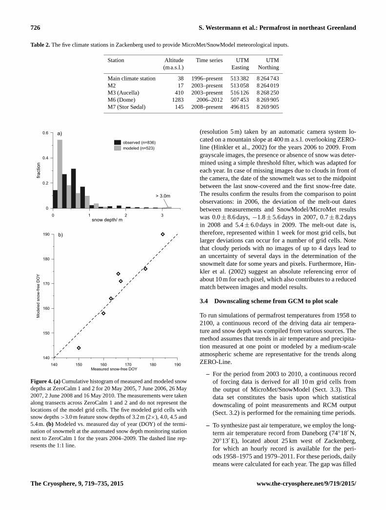
Figure 4. (a) Cumulative histogram of measured and modeled snow
depths at ZeroCalm 1 and 2 for 20 May 2005, 7 June 2006, 26 May
2007, 2 June 2008 and 16 May 2010. The measurements were taken
along transects across ZeroCalm 1 and 2 and do not represent the
locations of the model grid cells. The five modeled grid cells with
snow depths >3.0m feature snow depths of 3.2m (2×), 4.0, 4.5 and
5.4m. (b) Modeled vs. measured day of year (DOY) of the termi-
nation of snowmelt at the automated snow depth monitoring station
next to ZeroCalm 1 for the years 2004–2009. The dashed line rep-
resents the 1:1 line.
(resolution 5m) taken by an automatic camera system lo-
cated on a mountain slope at 400 m a.s.l. overlooking ZERO-
line (Hinkler et al., 2002) for the years 2006 to 2009. From
grayscale images, the presence or absence of snow was deter-
mined using a simple threshold filter, which was adapted for
each year. In case of missing images due to clouds in front of
the camera, the date of the snowmelt was set to the midpoint
between the last snow-covered and the first snow-free date.
The results confirm the results from the comparison to point
observations: in 2006, the deviation of the melt-out dates
between measurements and SnowModel/MicroMet results
was 0.0± 8.6days, −1.8± 5.6days in 2007, 0.7± 8.2days
in 2008 and 5.4± 6.0days in 2009. The melt-out date is,
therefore, represented within 1 week for most grid cells, but
larger deviations can occur for a number of grid cells. Note
that cloudy periods with no images of up to 4 days lead to
an uncertainty of several days in the determination of the
snowmelt date for some years and pixels. Furthermore, Hin-
kler et al. (2002) suggest an absolute referencing error of
about 10m for each pixel, which also contributes to a reduced
match between images and model results.
3.4 Downscaling scheme from GCM to plot scale
To run simulations of permafrost temperatures from 1958 to
2100, a continuous record of the driving data air tempera-
ture and snow depth was compiled from various sources. The
method assumes that trends in air temperature and precipita-
tion measured at one point or modeled by a medium-scale
atmospheric scheme are representative for the trends along
ZERO-Line.
– For the period from 2003 to 2010, a continuous record
of forcing data is derived for all 10 m grid cells from
the output of MicroMet/SnowModel (Sect. 3.3). This
data set constitutes the basis upon which statistical
downscaling of point measurements and RCM output
(Sect. 3.2) is performed for the remaining time periods.
– To synthesize past air temperature, we employ the long-
term air temperature record from Daneborg (74◦18′ N,
20◦13′ E), located about 25 km west of Zackenberg,
for which an hourly record is available for the peri-
ods 1958–1975 and 1979–2011. For these periods, daily
means were calculated for each year. The gap was filled
The Cryosphere, 9, 719–735, 2015 www.the-cryosphere.net/9/719/2015/

S. Westermann et al.: Permafrost in northeast Greenland 727
using random years selected from the 5 years before the
gap for the first half and the first 5 years after the gap
for its second half. In addition, a monthly trend was su-
perimposed on the randomly selected data, obtained by
linear interpolation between the monthly averages from
5 years before and 5 years after the gap. With this pro-
cedure, both a smooth transition between the time slices
and a simulated natural variability was achieved.
– For present-day and future air temperatures, the near-
surface air temperature from the HIRHAM5 5 km grid
cell closest to the study area, which are available for
three time slices, 1991–2010, 2031–2050 and 2081–
2100. The gaps in between the time slices were filled
similar to the gap in the Daneborg record.
– To account for differences in the climate setting be-
tween the study area and Daneborg/the HIRHAM grid
cell, we calculate the offset of the average air tem-
peratures between the Daneborg/HIRHAM records and
the MicroMet/SnowModel output for the period 2003–
2010, for which all time series are available simultane-
ously. A specific offset is calculated for each grid cell
and for each month of the year, thus accounting for both
the spatial gradients along Zero Line and the average
seasonal differences between the two sites.
– For both the past Daneborg and the future HIRHAM
time series, the difference to the monthly average of
the 2003–2010 reference period (i.e., a monthly time
series of offsets) was calculated. The final time se-
ries was synthesized by selecting air temperatures from
MicroMet/SnowModel for random years from 2003 to
2010 and subtracting the spatial and temporal offsets for
each grid cell and each month, respectively.
– Snow depths were obtained by a similar procedure.
Since a past record was not available and neither
snow depth nor winter snowfall modeled by HIRHAM
showed a significant trend, the snow depth was taken
from random years of the MicroMet/SnowModel pe-
riod (the same year as used for air temperatures) during
the buildup period. To model past and future snowmelt
in climate conditions different from the 2003–2010 Mi-
croMet/SnowModel period, a simple degree-day model
linking melt rates to air temperature (e.g., Hock, 2003)
was applied. We assumed a constant melt factor of
2.5 mm snow water equivalent per degree day for tem-
peratures exceeding −2 ◦C. The numbers were ob-
tained by fitting the snowmelt dates delivered by Mi-
croMet/SnowModel for the 437 10 m grid cells along
ZERO-line for the years 2003–2010. The average bias
in the snowmelt date of the degree-day melt model is
1.2 day compared to MicroMet/SnowModel. The abla-
tion of the snow cover was subsequently calculated us-
ing the downscaled air temperatures for each day. For air
temperatures colder than the MicroMet/SnowModel pe-
riod, this yields a later snowmelt, while the snow melts
earlier for warmer conditions.
4 Model results
4.1 Comparison to field data
To build confidence that the modeling is a satisfactory rep-
resentation for the true ground thermal conditions, the model
results are compared to available in situ data sets. These com-
prise in particular thaw depth measurements at ZeroCalm 1
and 2 since 1996, measurements of thaw depth along ZERO-
line in 2013 and measurements of ground temperatures con-
ducted in the active layer and the permafrost between 1996
and 2014 at 17 sites.
4.1.1 Active layer thickness
The modeled and measured maximum thaw depths for 7
years for which MicroMet/SnowModel was run are shown in
Fig. 5, with the areas selected for comparison equal to Elber-
ling et al. (2013). Most importantly, CryoGrid 2 can capture
the significant differences between the three sediment classes
Dryas, Cassiope and wetland caused by different ground and
surface properties. With a few exceptions, CryoGrid 2 can
reproduce the measured thaw depth within the spatial vari-
ability in the validation areas (indicated by the error bars
in Fig. 5), with the exception of the year 2006 which fea-
tures stronger deviations from the measurements. The spa-
tial variability within the target areas is significantly smaller
in the model runs than in nature, most likely since the sed-
iment classification assumes constant soil properties within
each class, while the soil composition can vary significantly
within a class in reality.
On 26 August 2013, thaw depths were measured manually
along the modeled part of ZERO-line at intervals of 30–40m.
Although MicroMet/SnowModel data were not employed in
the modeling of this year, a comparison to modeled data is
meaningful to assess the general range and distribution of
thaw depths along ZERO-line. The measured and modeled
distributions of thaw depths are displayed in Fig. 6. Although
thaw depths deeper than 1.0m could not be measured in the
field, the comparison shows that the modeling can generally
reproduce the range of thaw depths. Furthermore, the mod-
eled and measured fractions of thaw depths larger than 1.0m
are approximately equal. All model grid cells with such large
thaw depths belong to the class fell, which is an indication
that the modeling procedure is adequate also for fell. For
thaw depths between 0.4 and 0.7m, differences in the mod-
eled fractions occur (Fig. 6). However, this can be explained
by deviations between measured and modeled thaw depth on
the order of 0.1 to 0.2m, which is in agreement with the com-
parison of Fig. 5.
www.the-cryosphere.net/9/719/2015/ The Cryosphere, 9, 719–735, 2015
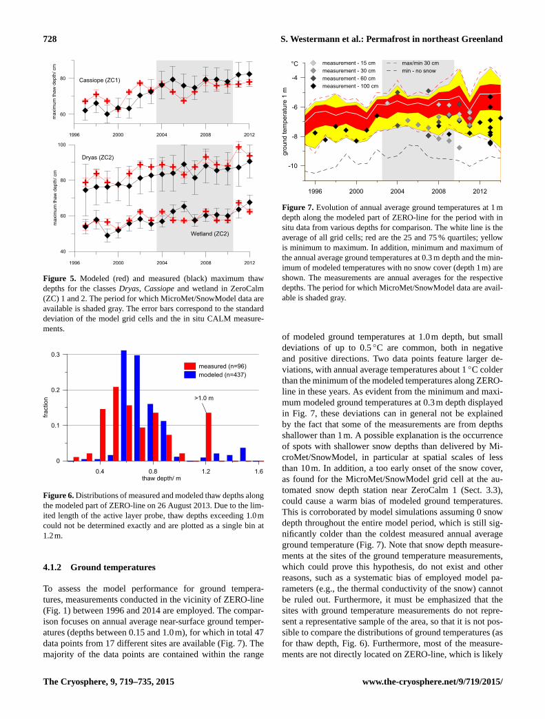
728 S. Westermann et al.: Permafrost in northeast Greenland
Figure 5. Modeled (red) and measured (black) maximum thaw
depths for the classes Dryas, Cassiope and wetland in ZeroCalm
(ZC) 1 and 2. The period for which MicroMet/SnowModel data are
available is shaded gray. The error bars correspond to the standard
deviation of the model grid cells and the in situ CALM measure-
ments.
Figure 6. Distributions of measured and modeled thaw depths along
the modeled part of ZERO-line on 26 August 2013. Due to the lim-
ited length of the active layer probe, thaw depths exceeding 1.0m
could not be determined exactly and are plotted as a single bin at
1.2m.
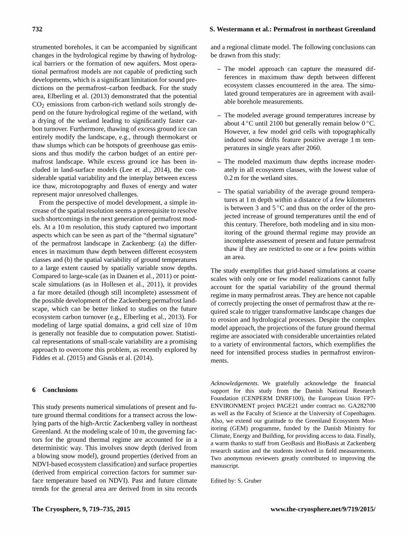
4.1.2 Ground temperatures
To assess the model performance for ground tempera-
tures, measurements conducted in the vicinity of ZERO-line
(Fig. 1) between 1996 and 2014 are employed. The compar-
ison focuses on annual average near-surface ground temper-
atures (depths between 0.15 and 1.0m), for which in total 47
data points from 17 different sites are available (Fig. 7). The
majority of the data points are contained within the range
Figure 7. Evolution of annual average ground temperatures at 1 m
depth along the modeled part of ZERO-line for the period with in
situ data from various depths for comparison. The white line is the
average of all grid cells; red are the 25 and 75 % quartiles; yellow
is minimum to maximum. In addition, minimum and maximum of
the annual average ground temperatures at 0.3 m depth and the min-
imum of modeled temperatures with no snow cover (depth 1m) are
shown. The measurements are annual averages for the respective
depths. The period for which MicroMet/SnowModel data are avail-
able is shaded gray.
of modeled ground temperatures at 1.0m depth, but small
deviations of up to 0.5 ◦C are common, both in negative
and positive directions. Two data points feature larger de-
viations, with annual average temperatures about 1 ◦C colder
than the minimum of the modeled temperatures along ZERO-
line in these years. As evident from the minimum and maxi-
mum modeled ground temperatures at 0.3m depth displayed
in Fig. 7, these deviations can in general not be explained
by the fact that some of the measurements are from depths
shallower than 1m. A possible explanation is the occurrence
of spots with shallower snow depths than delivered by Mi-
croMet/SnowModel, in particular at spatial scales of less
than 10m. In addition, a too early onset of the snow cover,
as found for the MicroMet/SnowModel grid cell at the au-
tomated snow depth station near ZeroCalm 1 (Sect. 3.3),
could cause a warm bias of modeled ground temperatures.
This is corroborated by model simulations assuming 0 snow
depth throughout the entire model period, which is still sig-
nificantly colder than the coldest measured annual average
ground temperature (Fig. 7). Note that snow depth measure-
ments at the sites of the ground temperature measurements,
which could prove this hypothesis, do not exist and other
reasons, such as a systematic bias of employed model pa-
rameters (e.g., the thermal conductivity of the snow) cannot
be ruled out. Furthermore, it must be emphasized that the
sites with ground temperature measurements do not repre-
sent a representative sample of the area, so that it is not pos-
sible to compare the distributions of ground temperatures (as
for thaw depth, Fig. 6). Furthermore, most of the measure-
ments are not directly located on ZERO-line, which is likely
The Cryosphere, 9, 719–735, 2015 www.the-cryosphere.net/9/719/2015/

S. Westermann et al.: Permafrost in northeast Greenland 729
S. Westermann et al.: Permafrost in NE Greenland 13
Figure 8. Evolution of annual average ground temperatures at 1m (top) and 10m (bottom) depth along the modeled part of ZERO-line until2100. White line: average of all grid cells; Red: 25 and 75 % quartiles; yellow: minimum to maximum.Figure 8. Evolution of annual average ground temperatures at 1 m
(top) and 10 m (bottom) depth along the modeled part of ZERO-line
until 2100. The white line is the average of all grid cells; red are the
25 and 75 % quartiles; yellow is minimum to maximum.
to cause additional deviations between measurements and
model results. Nevertheless, the comparison suggests that the
modeling approach is able to capture the spatial variability of
near-surface ground temperatures along and in the vicinity of
ZERO-line.
In deeper layers, ground temperatures are influenced by
the temperature forcing of an extended period prior to the
measurement. Therefore, measurements in deep boreholes
are especially well suited to check the long-term performance
of a ground thermal model (in this case the model spin-up
produced by statistical downscaling). In 2012, the two deep
boreholes in the Zackenberg area featured temperatures at
10 m depth of −5.2 ◦C at a site with a snowdrift and −6.7 ◦C
at the meteorological station with more regular snow con-
ditions. These point measurements are well in the range of
10 m temperatures delivered by CryoGrid 2 along ZERO-line
in 2012, (−6.0± 0.6) ◦C, and maximum and minimum tem-
peratures of −5.1 and −8.0 ◦C. The satisfactory agreement
suggests that the statistical downscaling procedure (Sect. 3.4)
employed to produce the forcing data for the model spin-up
is adequate for the area.
Figure 9. Evolution of annual maximum thaw depth until 2100 for
the ecosystem classes Cassiope (ZeroCalm 1), Dryas and wetland
(ZeroCalm 2). The yellow areas indicate the range of modeled max-
imum thaw depths.
4.2 Evolution of active layer thickness and ground
temperatures
The modeled evolution of the temperature distribution at 1 m
depth along ZERO-line is shown in Fig. 8. The modeled tem-
peratures extend over a range of 2 to 5 ◦C from minimum to
maximum which is evidence of the significant spatial vari-
ability of the ground thermal regime in this landscape. In
order to investigate the sources for this spatial variability, a
sensitivity analysis was performed by running CryoGrid 2
for ZERO-line with a uniform ground stratigraphy and asso-
ciated characteristic NDVI values (Sect. 3.1) for each of the
four stratigraphic classes: fell, Dryas, Cassiope and wetland.
This analysis suggests that snow depth has the largest ef-
fect on 1m ground temperatures, with a variability 3–5 times
larger than that caused by ground and surface properties.
However, modeled maximum thaw depths are much more
influenced by ground and surface properties than by snow
depths, which only lead to differences on the order of 0.1 to
0.2m compared to differences of more than 0.5m for differ-
ent stratigraphic classes/NDVI values. A statistically signifi-
cant correlation between NDVI values (and thus stratigraphic
classes) and snow depths modeled by SnowModel/MicroMet
does not exist in the employed data set.
According to the climate change scenario of the future
projections (Sect. 3.2), ground temperatures will warm by
about 4 ◦C until 2100, but permafrost will largely remain
thermally sustainable along ZERO-line. However, the high-
resolution simulations suggest a few sites where the yearly
average 1m ground temperatures become positive in some
years at the end of this century (Fig. 8). These sites are char-
acterized by above-average snow depths in the long-term av-
erage, which suggests that talik formation may be initiated
www.the-cryosphere.net/9/719/2015/ The Cryosphere, 9, 719–735, 2015

730 S. Westermann et al.: Permafrost in northeast Greenland
at sites with topographically induced snowdrifts. The future
warming of air temperatures predicted by HIRHAM is not
constant over the year, with the most pronounced warming
of 0.4–0.6 ◦C per decade occurring in fall, winter and spring,
while summer (June to August) temperatures increase by less
than 0.2 ◦C per decade. As a consequence, the annual maxi-
mum thaw depths increase only moderately until 2100, from
0.8–1.0 to 1.1–1.4 m for Dryas, from 0.65–0.85 to 0.8–1.1 m
for Cassiope and from 0.5–0.65 to 0.6–0.8 m for the wet-
land class (Fig. 9). The climate sensitivity of thaw depths is
different between the classes, with a stronger increase for the
classes with dryer soils than for the wetlands. It is remarkable
that the projected increase is only 0.1–0.2 m in the wetlands,
which can be related to the high ice content in the frozen
active layer and to relatively smaller increase in summer sur-
face temperatures due to the low summer nt factors assigned
to the wetland class (Fig. 3).
The biological activity in this high-Arctic ecosystem is
strongly related to summer conditions. The simulations sug-
gest a significant increase in average summer temperatures
and thawing degree days (Fig. 10) within the effective root
depth. The combination of deeper active layer (Fig. 9) and
warmer near-surface (Fig. 10) summer conditions is an im-
portant control for plant growth. Water and nutrients (mainly
nitrogen) are being released from the thawing permafrost,
and the longer growing season and warmer top soil condi-
tions allow plants to benefit from the additional nutrient and
result in changes in the competition among plant species for
light. This may lead to marked changes in vegetation over
time, but this is beyond the scope of this study.
5 Discussion
5.1 Scaling strategies from GCM to plot scale
The presented simulations of ground temperatures and per-
mafrost state variables are derived from a multi-step down-
scaling approach (Sect. 3.4) which bridges the coarse spa-
tial resolution of a GCM (hundreds of km) and the impact
scale on the ground (set to 10 m for this study). As such,
the scheme is technically capable of bridging 5 to 6 orders
of magnitude in space. The two main driving environmen-
tal variables for the thermal model CryoGrid 2 are surface
temperature and snow depth.
The snow depth is assumed to be controlled by wind
drift of snow at the target scale of 10 m which is modeled
by the snow redistribution scheme MicroMet/SnowModel.
MicroMet/SnowModel is a deterministic scheme capable of
predicting the snow depth for each model grid cell, thus re-
producing the location of snow drifts and bare-blown spots.
Such deterministic high-resolution modeling facilitates a bet-
ter comparison and validation with ground observations but
is restricted to small model domains for computational rea-
sons. However, SnowModel also includes the ability to sim-
S. Westermann et al.: Permafrost in NE Greenland 15
Figure 10. The distribution of thawing degree days (top) and average summer (June–August) temperatures (bottom) at 0.1m depth alongZERO-line until 2100.
Figure 10. The distribution of thawing degree days (top) and av-
erage summer (June–August) temperatures (bottom) at 0.1 m depth
along ZERO-line until 2100.
ulate snow distributions over large areas (e.g., the ice-free
parts of Greenland, several 100 000 km2) using, for example,
subgrid snow distribution representations (e.g., Liston et al.,
1999; Liston, 2004; Liston and Hiemstra, 2011). Gisnås et al.
(2014) recently presented a statistical approach to account
for the impact of the small-scale variability of snow depths
on ground temperatures that is applicable on large spatial do-
mains.
The surface temperature is derived from air temperature
for which the regional gradients are based on the RCM at
a scale of 5 km. Within the target area along ZERO-line (a
distance of 4 km), variations in air temperature are generally
small. Further downscaling to 10 m is accomplished by us-
ing a high-resolution NDVI satellite image and the NDVI
vs. n factor relationship (Sect. 3.1) which is used to con-
vert air to surface temperatures during the snow-free season.
By this scheme, a high-resolution data set of surface tem-
peratures is generated from comparatively low-resolution air
temperature data. More physically based approaches make
use of the surface energy balance (SEB) to compute surface
temperatures from air temperature, wind speed, humidity and
The Cryosphere, 9, 719–735, 2015 www.the-cryosphere.net/9/719/2015/

S. Westermann et al.: Permafrost in northeast Greenland 731
incoming radiation (e.g., Zhang et al., 2013; Fiddes et al.,
2015). In addition to accounting for more complex topog-
raphy through spatially distributed fields of incoming radi-
ation, the surface energy balance and thus the surface tem-
perature can directly be connected to surface soil moisture
and land cover/vegetation type, which circumvents the use of
n factors. Nonetheless, SEB models require additional driv-
ing data sets, in particular incoming radiation, which must be
compiled, e.g., from large-scale atmospheric modeling (Fid-
des and Gruber, 2014) and/or from sparse in situ measure-
ments (Zhang et al., 2012). Due to the potential for serious
biases in such driving data sets in remote locations (such as
Zackenberg), it remains unclear whether the capacity of SEB
models in reproducing the true surface temperature is supe-
rior to the simple empirical concept employed in this study.
5.2 Model uncertainty
The presented model results must be considered a first-order
approximation of the future thermal state of the permafrost,
which is subject to considerable uncertainty due to a variety
of factors. Firstly, only one climate change scenario is con-
sidered, which does not account for the considerable spread
in climate predictions. With permafrost approaching the thaw
threshold at the end of this century for RCP 4.5 forcing,
wide-spread permafrost degradation is e.g., likely for more
aggressive climate change scenarios.
Secondly, the downscaling procedure from large-scale
model data to high-resolution fields of temperature and snow
depth is susceptible to uncertainties, since it assumes con-
stant offsets between the two data sets based on the climate
conditions of a 7-year reference period, which may not be
justified for a 100-year period. This is particularly critical
since the temperature regime in the study area is character-
ized by strong inversion settings during a large part of the
year (Meltofte et al., 2008). A modification of such inver-
sions could lead to a different climate susceptibility of the
study area compared to the large-scale trend, which cannot
be captured during the reference period. Furthermore, the fu-
ture snow distribution patterns are based on random years
from the 7-year reference period, implying that the patterns
are unchanged in a warmer future climate and that the ref-
erence period allows a representative sample of the interan-
nual variability within the rest of the century. It is not un-
likely that both assumptions are violated at least to a cer-
tain degree. In addition, new processes not accounted for by
the modeling scheme might become relevant in the course
of climate warming, e.g., the occurrence of wintertime rain
events, which can lead to significant additional ground warm-
ing (Westermann et al., 2011).
The CryoGrid 2 permafrost model assumes properties and
relationships compiled and adjusted for the present state to
be valid in the future. This concerns in particular the NDVI-
based summer n-factor relationship employed to derive sur-
face from air temperatures (Sect. 3.1), as well the thermal
properties of the snow and the ground stratigraphy. As an ex-
ample, the snow density and thermal conductivity are likely
to increase in a warmer climate, which would decrease the
insulation of the winter snow cover and thus lead to colder
temperatures, as suggested by the model. A sensitivity study
for a transient thermal model similar to CryoGrid 2 in Siberia
showed that the thermal properties of the snow cover are
the critical source of uncertainty for successfully reproduc-
ing ground temperatures (Langer et al., 2013). A similar re-
sult was found in a sensitivity study with GEOtop (Endrizzi
et al., 2014) for a site in the European Alps for which the
assumed snow conditions crucially influenced the uncertain-
ties of modeled ground temperatures (Gubler et al., 2013).
Most likely, these findings are also applicable to this study
and the representation of the snow cover (including snow
water equivalent, density and thermal conductivity) deserves
increased attention in future modeling approaches. However,
the ground thermal properties related to the ground stratigra-
phy proved to be the crucial source of uncertainty regarding
modeled thaw depths (Langer et al., 2013). In this study, con-
stant soil water and ice contents are assumed in our model-
ing, thus neglecting both seasonal and long-term changes in
the water cycle. However, at least for the Cassiope class, our
results for the future increase in maximum thaw depth are
in good agreement with the study of Hollesen et al. (2011)
who used the coupled heat and water transfer model COUP
(Jansson and Karlberg, 2004) to simulate the ground thermal
and moisture regimes in this century. While a coupled energy
and water cycle is implemented in a number of modeling
schemes, such as GEOtop (Endrizzi et al., 2014) or Surfex
(Masson et al., 2013), a major challenge is modeling lateral
water fluxes, which create spatially different soil moisture
conditions (as at the Zackenberg site) that subsequently can
have a pronounced impact on the ground thermal regime.
As pointed out by Gubler et al. (2011), spatially distributed
in situ data sets are required to calibrate and validate spatially
distributed modeling schemes in heterogeneous permafrost
landscapes. These should capture the variability of the dif-
ferent environmental factors governing the ground thermal
regime, which in many permafrost landscapes will require a
significant effort with potentially dozens of measurement lo-
cations. However, such work is a crucial prerequisite to im-
prove the ability of modeling schemes to simulate the dis-
tribution of the ground thermal regime and its response to
present and future changes.
5.3 From model results to permafrost landscape
development
Most real-world applications of permafrost models assume
non-interacting grid cells with spatially constant soil proper-
ties. Consequently, permafrost degradation in model studies
(e.g., Westermann et al., 2013) is generally described as talik
formation manifested in the temperature profile of a one-
dimensional grid cell. While this is indeed observed in in-
www.the-cryosphere.net/9/719/2015/ The Cryosphere, 9, 719–735, 2015
732 S. Westermann et al.: Permafrost in northeast Greenland
strumented boreholes, it can be accompanied by significant
changes in the hydrological regime by thawing of hydrolog-
ical barriers or the formation of new aquifers. Most opera-
tional permafrost models are not capable of predicting such
developments, which is a significant limitation for sound pre-
dictions on the permafrost–carbon feedback. For the study
area, Elberling et al. (2013) demonstrated that the potential
CO2 emissions from carbon-rich wetland soils strongly de-
pend on the future hydrological regime of the wetland, with
a drying of the wetland leading to significantly faster car-
bon turnover. Furthermore, thawing of excess ground ice can
entirely modify the landscape, e.g., through thermokarst or
thaw slumps which can be hotspots of greenhouse gas emis-
sions and thus modify the carbon budget of an entire per-
mafrost landscape. While excess ground ice has been in-
cluded in land-surface models (Lee et al., 2014), the con-
siderable spatial variability and the interplay between excess
ice thaw, microtopography and fluxes of energy and water
represent major unresolved challenges.
From the perspective of model development, a simple in-
crease of the spatial resolution seems a prerequisite to resolve
such shortcomings in the next generation of permafrost mod-
els. At a 10 m resolution, this study captured two important
aspects which can be seen as part of the “thermal signature”
of the permafrost landscape in Zackenberg: (a) the differ-
ences in maximum thaw depth between different ecosystem
classes and (b) the spatial variability of ground temperatures
to a large extent caused by spatially variable snow depths.
Compared to large-scale (as in Daanen et al., 2011) or point-
scale simulations (as in Hollesen et al., 2011), it provides
a far more detailed (though still incomplete) assessment of
the possible development of the Zackenberg permafrost land-
scape, which can be better linked to studies on the future
ecosystem carbon turnover (e.g., Elberling et al., 2013). For
modeling of large spatial domains, a grid cell size of 10m
is generally not feasible due to computation power. Statisti-
cal representations of small-scale variability are a promising
approach to overcome this problem, as recently explored by
Fiddes et al. (2015) and Gisnås et al. (2014).
6 Conclusions
This study presents numerical simulations of present and fu-
ture ground thermal conditions for a transect across the low-
lying parts of the high-Arctic Zackenberg valley in northeast
Greenland. At the modeling scale of 10 m, the governing fac-
tors for the ground thermal regime are accounted for in a
deterministic way. This involves snow depth (derived from
a blowing snow model), ground properties (derived from an
NDVI-based ecosystem classification) and surface properties
(derived from empirical correction factors for summer sur-
face temperature based on NDVI). Past and future climate
trends for the general area are derived from in situ records
and a regional climate model. The following conclusions can
be drawn from this study:
– The model approach can capture the measured dif-
ferences in maximum thaw depth between different
ecosystem classes encountered in the area. The simu-
lated ground temperatures are in agreement with avail-
able borehole measurements.
– The modeled average ground temperatures increase by
about 4 ◦C until 2100 but generally remain below 0 ◦C.
However, a few model grid cells with topographically
induced snow drifts feature positive average 1 m tem-
peratures in single years after 2060.
– The modeled maximum thaw depths increase moder-
ately in all ecosystem classes, with the lowest value of
0.2 m for the wetland sites.
– The spatial variability of the average ground tempera-
tures at 1 m depth within a distance of a few kilometers
is between 3 and 5 ◦C and thus on the order of the pro-
jected increase of ground temperatures until the end of
this century. Therefore, both modeling and in situ mon-
itoring of the ground thermal regime may provide an
incomplete assessment of present and future permafrost
thaw if they are restricted to one or a few points within
an area.
The study exemplifies that grid-based simulations at coarse
scales with only one or few model realizations cannot fully
account for the spatial variability of the ground thermal
regime in many permafrost areas. They are hence not capable
of correctly projecting the onset of permafrost thaw at the re-
quired scale to trigger transformative landscape changes due
to erosion and hydrological processes. Despite the complex
model approach, the projections of the future ground thermal
regime are associated with considerable uncertainties related
to a variety of environmental factors, which exemplifies the
need for intensified process studies in permafrost environ-
ments.
Acknowledgements. We gratefully acknowledge the financial
support for this study from the Danish National Research
Foundation (CENPERM DNRF100), the European Union FP7-
ENVIRONMENT project PAGE21 under contract no. GA282700
as well as the Faculty of Science at the University of Copenhagen.
Also, we extend our gratitude to the Greenland Ecosystem Mon-
itoring (GEM) programme, funded by the Danish Ministry for
Climate, Energy and Building, for providing access to data. Finally,
a warm thanks to staff from GeoBasis and BioBasis at Zackenberg
research station and the students involved in field measurements.
Two anonymous reviewers greatly contributed to improving the
manuscript.
Edited by: S. Gruber
The Cryosphere, 9, 719–735, 2015 www.the-cryosphere.net/9/719/2015/

S. Westermann et al.: Permafrost in northeast Greenland 733
References
Bay, C.: Vegetation mapping of Zackenberg valley, Northeast
Greenland, Danish Polar Center and Botanical Museum, Univer-
sity of Copenhagen, 75 pp., 1998.
Brown, J., Hinkel, K., and Nelson, F.: The circumpolar active layer
monitoring (CALM) program: research designs and initial re-
sults, Polar Geogr., 24, 166–258, 2000.
Christensen, J. H., Christensen, O. B., Lopez, P., van Meijgaard, E.,
and Botzet, M.: The HIRHAM 4 regional atmospheric climate
model, Scientific Report 96-4, Danish Meteorological Institute,
51 pp., 1996.
Clarke, L., Edmonds, J., Jacoby, H., Pitcher, H., Reilly, J., and
Richels, R.: Scenarios of greenhouse gas emissions and atmo-
spheric concentrations, Sub-report of Synthesis and Assessment
Product – 2.1. Climate Change Science Program and the Sub-
committee on Global Change Research, Washington DC, 2007.
Clauser, C. and Huenges, E.: Thermal conductivity of rocks and
minerals, AGU Reference Shelf, 3, 105–126, 1995.
Cosenza, P., Guerin, R., and Tabbagh, A.: Relationship between
thermal conductivity and water content of soils using numerical
modelling, European J. Soil Sci., 54, 581–588, 2003.
Côté, J. and Konrad, J.-M.: A generalized thermal conductivity
model for soils and construction materials, Canad. Geotechn. J.,
42, 443–458, 2005.
Daanen, R. P., Ingeman-Nielsen, T., Marchenko, S. S., Ro-
manovsky, V. E., Foged, N., Stendel, M., Christensen, J. H.,
and Hornbech Svendsen, K.: Permafrost degradation risk zone
assessment using simulation models, The Cryosphere, 5, 1043–
1056, doi:10.5194/tc-5-1043-2011, 2011.
Dall’Amico, M., Endrizzi, S., Gruber, S., and Rigon, R.: A robust
and energy-conserving model of freezing variably-saturated soil,
The Cryosphere, 5, 469–484, doi:10.5194/tc-5-469-2011,2011.
Elberling, B., Jakobsen, B. H., Berg, P., Søndergaard, J., and Sigs-
gaard, C.: Influence of vegetation, temperature, and water content
on soil carbon distribution and mineralization in four High Arctic
soils, Arct. Antarct. Alp. Res., 36, 528–538, 2004.
Elberling, B., Tamstorf, M. P., Michelsen, A., Arndal, M. F., Sigs-
gaard, C., Illeris, L., Bay, C., Hansen, B. U., Christensen, T. R.,
Hansen, E. S., Jakobsen, B. H., and Beyens, L.: Soil and plant
community-characteristics and dynamics at Zackenberg, Adv.
Ecol. Res., 40, 223–248, 2008.
Elberling, B., Christiansen, H. H., and Hansen, B. U.: High nitrous
oxide production from thawing permafrost, Nature Geosci., 3,
332–335, 2010.
Elberling, B., Michelsen, A., Schädel, C., Schuur, E. A., Chris-
tiansen, H. H., Berg, L., Tamstorf, M. P., and Sigsgaard, C.:
Long-term CO2 production following permafrost thaw, Nature
Clim. Change, 3, 890–894, 2013.
Ellebjerg, S. M., Tamstorf, M. P., Illeris, L., Michelsen, A., and
Hansen, B. U.: Inter-annual variability and controls of plant phe-
nology and productivity at Zackenberg, Adv. Ecol. Res., 40, 249–
273, 2008.
Endrizzi, S., Gruber, S., Dall’Amico, M., and Rigon, R.: GEOtop
2.0: simulating the combined energy and water balance at
and below the land surface accounting for soil freezing, snow
cover and terrain effects, Geosci. Model Dev., 7, 2831–2857,
doi:10.5194/gmd-7-2831-2014, 2014.
Fiddes, J. and Gruber, S.: TopoSUB: a tool for efficient large area
numerical modelling in complex topography at sub-grid scales,
Geosci. Model Dev., 5, 1245–1257, doi:10.5194/gmd-5-1245-
2012, 2012.
Fiddes, J. and Gruber, S.: TopoSCALE v.1.0: downscaling gridded
climate data in complex terrain, Geosci. Model Dev., 7, 387–405,
doi:10.5194/gmd-7-387-2014, 2014.
Fiddes, J., Endrizzi, S., and Gruber, S.: Large-area land surface sim-
ulations in heterogeneous terrain driven by global data sets: ap-
plication to mountain permafrost, The Cryosphere, 9, 411–426,
doi:10.5194/tc-9-411-2015, 2015.
Fredskild, B. and Mogensen, G. S.: Zero Line: Final Report 1997:
a Description of the Plant Communities Along the ZERO Line
from Young Sund to the Top of Aucellabjerg and the Common
Plant Communities in the Zackenberg Valley, Northeast Green-
land, Greenland Botanical Survey & Botanical Museum, Univer-
sity of Copenhagen, 1997.
Gisnås, K., Westermann, S., Schuler, T. V., Litherland, T., Isaksen,
K., Boike, J., and Etzelmüller, B.: A statistical approach to rep-
resent small-scale variability of permafrost temperatures due to
snow cover, The Cryosphere, 8, 2063–2074, doi:10.5194/tc-8-
2063-2014, 2014.
Goodrich, L.: The influence of snow cover on the ground thermal
regime, Canad. Geotech. J., 19, 421–432, 1982.
Gubler, S., Fiddes, J., Keller, M., and Gruber, S.: Scale-
dependent measurement and analysis of ground surface temper-
ature variability in alpine terrain, The Cryosphere, 5, 431–443,
doi:10.5194/tc-5-431-2011, 2011.
Gubler, S., Endrizzi, S., Gruber, S., and Purves, R. S.: Sensi-
tivities and uncertainties of modeled ground temperatures in
mountain environments, Geosci. Model Dev., 6, 1319–1336,
doi:10.5194/gmd-6-1319-2013, 2013.
Hansen, B. U., Sigsgaard, C., Rasmussen, L., Cappelen, J., Hinkler,
J., Mernild, S. H., Petersen, D., Tamstorf, M. P., Rasch, M., and
Hasholt, B.: Present-day climate at Zackenberg, Adv. Ecol. Res.,
40, 111–149, 2008.
Hazeleger, W., Severijns, C., Semmler, T., Stefanescu, S., Yang,
S., Wang, X., Wyser, K., Dutra, E., Baldasano, J. M., Bin-
tanja, R., Caballero, R., Dutra, E., Ekman, A., Christensen, J.,
van den Hurk, B., Jimenez, P., Jones, C., Kallberg, P., McGrath,
R., de Miranda, P., Molteni, F., van Noije, T., Palmer, T., Ro-
driguez Camino, E., Schmith, T., Selten, T., Sterl, A., Tapamo,
H., and Viterbo, P.: EC-earth: a seamless earth-system prediction
approach in action, B. Am. Meteor. Soc., 91, 1357–1363, 2010.
Hazeleger, W., Wang, X., Severijns, C., Stefanescu, S., Bintanja,
R., Sterl, A., Wyser, K., Semmler, T., Yang, S., Van den Hurk,
B., van Noije, T., van der Linden, E., and van der Wiel, K.: EC-
Earth V2. 2: description and validation of a new seamless earth
system prediction model, Clim. Dynam., 39, 2611–2629, 2012.
Hinkler, J., Pedersen, S. B., Rasch, M., and Hansen, B. U.: Auto-
matic snow cover monitoring at high temporal and spatial reso-
lution, using images taken by a standard digital camera, Int. J.
Remote Sens., 23, 4669–4682, 2002.
Hipp, T., Etzelmüller, B., Farbrot, H., Schuler, T., and Westermann,
S.: Modelling borehole temperatures in Southern Norway – in-
sights into permafrost dynamics during the 20th and 21st century,
The Cryosphere, 6, 553–571, doi:10.5194/tc-6-553-2012, 2012.
Hock, R.: Temperature index melt modelling in mountain areas, J.
Hydrol., 282, 104–115, 2003.
Hollesen, J., Elberling, B., and Jansson, P. E.: Future active layer dy-
namics and carbon dioxide production from thawing permafrost
www.the-cryosphere.net/9/719/2015/ The Cryosphere, 9, 719–735, 2015
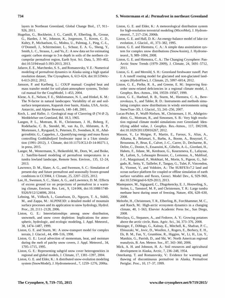
734 S. Westermann et al.: Permafrost in northeast Greenland
layers in Northeast Greenland, Global Change Biol., 17, 911–
926, 2011.
Hugelius, G., Bockheim, J. G., Camill, P., Elberling, B., Grosse,
G., Harden, J. W., Johnson, K., Jorgenson, T., Koven, C. D.,
Kuhry, P., Michaelson, G., Mishra, U., Palmtag, J., Ping, C.-L.,
O’Donnell, J., Schirrmeister, L., Schuur, E. A. G., Sheng, Y.,
Smith, L. C., Strauss, J., and Yu, Z.: A new data set for estimating
organic carbon storage to 3 m depth in soils of the northern cir-
cumpolar permafrost region, Earth Syst. Sci. Data, 5, 393–402,
doi:10.5194/essd-5-393-2013, 2013.
Jafarov, E. E., Marchenko, S. S., and Romanovsky, V. E.: Numerical
modeling of permafrost dynamics in Alaska using a high spatial
resolution dataset, The Cryosphere, 6, 613–624, doi:10.5194/tc-
6-613-2012, 2012.
Jansson, P. and Karlberg, L.: COUP manual: Coupled heat and
mass transfer model for soil-plant-atmosphere systems, Techni-
cal manual for the CoupModel, 1–453, 2004.
Klene, A. E., Nelson, F. E., Shiklomanov, N. I., and Hinkel, K. M.:
The N-factor in natural landscapes: Variability of air and soil-
surface temperatures, Kuparuk river basin, Alaska, USA, Arctic,
Antarctic, and Alpine Research, 140–148, 2001.
Koch, L. and Haller, J.: Geological map of Clavering Ø (74 Ø 2),
Meddelelser om Grønland, Bd. 18.3, 1965.
Langen, P. L., Mottram, R. H., Christensen, J. H., Boberg, F.,
Rodehacke, C. B., Stendel, M., van As, D., Ahlstrøm, A. P.,
Mortensen, J., Rysgaard, S., Petersen, D., Svendsen, K. H., Aðal-
geirsdóttir, G., Cappelen, J., Quantifying energy and mass fluxes
controlling Godthåbsfjord freshwater input in a 5 km simula-
tion (1991–2012), J. Climate, doi:10.1175/JCLI-D-14-00271.1,
in press, 2015.
Langer, M., Westermann, S., Heikenfeld, M., Dorn, W., and Boike,
J.: Satellite-based modeling of permafrost temperatures in a
tundra lowland landscape, Remote Sens. Environ., 135, 12–24,
2013.
Lawrence, D. M., Slater, A. G., and Swenson, S. C.: Simulation of
present-day and future permafrost and seasonally frozen ground
conditions in CCSM4, J. Climate, 25, 2207–2225, 2012.
Lee, H., Swenson, S. C., Slater, A. G., and Lawrence, D. M.: Effects
of excess ground ice on projections of permafrost in a warm-
ing climate, Environ. Res. Lett., 9, 124 006, doi:10.1088/1748-
9326/9/12/124006, 2014.
Lehning, M., Völksch, I., Gustafsson, D., Nguyen, T. A., Stähli,
M., and Zappa, M.: ALPINE3D: a detailed model of mountain
surface processes and its application to snow hydrology, Hydrol.
Proc., 20, 2111–2128, 2006.
Liston, G. E.: Interrelationships among snow distribution,
snowmelt, and snow cover depletion: Implications for atmo-
spheric, hydrologic, and ecologic modeling, J. Appl. Meteorol.,
38, 1474–1487, 1999.
Liston, G. E. and Sturm, M.: A snow-transport model for complex
terrain, J. Glaciol., 44, 498–516, 1998.
Liston, G. E.: Local advection of momentum, heat, and moisture
during the melt of patchy snow covers, J. Appl. Meteorol., 34,
1705–1715, 1995.
Liston, G. E.: Representing subgrid snow cover heterogeneities in
regional and global models, J. Climate, 17, 1381–1397, 2004.
Liston, G. E. and Elder, K.: A distributed snow-evolution modeling
system (SnowModel), J. Hydrometeorol., 7, 1259–1276, 2006a.
Liston, G. E. and Elder, K.: A meteorological distribution system
for high-resolution terrestrial modeling (MicroMet), J. Hydrom-
eteorol., 7, 217–234, 2006b.
Liston, G. E. and Hall, D. K.: An energy-balance model of lake-ice
evolution, J. Glaciol., 41, 373–382, 1995.
Liston, G. E. and Hiemstra, C. A.: A simple data assimilation sys-
tem for complex snow distributions (SnowAssim), J. Hydrome-
teorol., 9, 989–1004, 2008.
Liston, G. E. and Hiemstra, C. A.: The Changing Cryosphere: Pan-
Arctic Snow Trends (1979–2009), J. Climate, 24, 5691–5712,
2011.
Liston, G. E. and Mernild, S. H.: Greenland freshwater runoff. Part
I: A runoff routing model for glaciated and non-glaciated land-
scapes (HydroFlow), J. Climate, 25, 5997–6014, 2012.
Liston, G. E., Pielke, R. A., and Greene, E. M.: Improving first-
order snow-related deficiencies in a regional climate model, J.
Geophys. Res.-Atmos., 104, 19559–19567, 1999.
Liston, G. E., Haehnel, R. B., Sturm, M., Hiemstra, C. A., Bere-
zovskaya, S., and Tabler, R. D.: Instruments and methods simu-
lating complex snow distributions in windy environments using
SnowTran–3D, J. Glaciol., 53, 241–256, 2007.
Lucas-Picher, P., Wulff-Nielsen, M., Christensen, J. H., Aðalgeirs-
dóttir, G., Mottram, R., and Simonsen, S. B.: Very high resolu-
tion regional climate model simulations over Greenland: Iden-
tifying added value, J. Geophys. Res.-Atmos., 117, D02108,
doi:10.1029/2011JD016267, 2012.
Masson, V., Le Moigne, P., Martin, E., Faroux, S., Alias, A.,
Alkama, R., Belamari, S., Barbu, A., Boone, A., Bouyssel, F.,
Brousseau, P., Brun, E., Calvet, J.-C., Carrer, D., Decharme, B.,
Delire, C., Donier, S., Essaouini, K., Gibelin, A.-L., Giordani, H.,
Habets, F., Jidane, M., Kerdraon, G., Kourzeneva, E., Lafaysse,
M., Lafont, S., Lebeaupin Brossier, C., Lemonsu, A., Mahfouf,
J.-F., Marguinaud, P., Mokhtari, M., Morin, S., Pigeon, G., Sal-
gado, R., Seity, Y., Taillefer, F., Tanguy, G., Tulet, P., Vincendon,
B., Vionnet, V., and Voldoire, A.: The SURFEXv7.2 land and
ocean surface platform for coupled or offline simulation of earth
surface variables and fluxes, Geosci. Model Dev., 6, 929–960,
doi:10.5194/gmd-6-929-2013, 2013.
Mastepanov, M., Sigsgaard, C., Dlugokencky, E. J., Houweling, S.,
Ström, L., Tamstorf, M. P., and Christensen, T. R.: Large tundra
methane burst during onset of freezing, Nature, 456, 628–630,
2008.
Meltofte, H., Christensen, T. R., Elberling, B., Forchhammer, M. C.,
and Rasch, M.: High-arctic ecosystem dynamics in a changing
climate, 40, 1–563, Elsevier Academic Press Inc., San Diego,
2008.
Merzlaya, G., Stepanov, A., and Fedorov, A. Y.: Growing potatoes
above the arctic circle, Russ. Agric. Sci., 34, 373–376, 2008.
Mesinger, F., DiMego, G., Kalnay, E., Mitchell, K., Shafran, P. C.,
Ebisuzaki, W., Jovic, D., Woollen, J., Rogers, E., Berbery, E. H.,
Ek, B. M., Fan, Y., Grumbine, R., Higgins, W., Li, H., Lin, Y.,
Manikin, G., Parrish, D., and Shi, W.: North American regional
reanalysis, B. Am. Meteor. Soc., 87, 343–360, 2006.
Mick, A. H. and Johnson, H. A.: Soil resources and agricultural
development in Alaska, Arctic, 7, 236–248, 1954.
Osterkamp, T. and Romanovsky, V.: Evidence for warming and
thawing of discontinuous permafrost in Alaska, Permafrost
Periglac. Proc., 10, 17–37, 1999.
The Cryosphere, 9, 719–735, 2015 www.the-cryosphere.net/9/719/2015/
S. Westermann et al.: Permafrost in northeast Greenland 735
Pedersen, S. H., Liston, G. E., Tamstorf, M. P., Westergaard-
Nielsen, A., and Schmidt, N. M.: Quantifying episodic snowmelt
events in Arctic ecosystems, Ecosystems, doi:10.1007/s10021-
015-9867-8, 2015.
Rae, J. G. L., Aðalgeirsdóttir, G., Edwards, T. L., Fettweis, X., Gre-
gory, J. M., Hewitt, H. T., Lowe, J. A., Lucas-Picher, P., Mot-
tram, R. H., Payne, A. J., Ridley, J. K., Shannon, S. R., van de
Berg, W. J., van de Wal, R. S. W., and van den Broeke, M. R.:
Greenland ice sheet surface mass balance: evaluating simula-
tions and making projections with regional climate models, The
Cryosphere, 6, 1275–1294, doi:10.5194/tc-6-1275-2012, 2012.
Schuur, E. A. G., Bockheim, J., Canadell, J. G., Euskirchen, E.,
Field, C. B., Goryachkin, S. V., Hagemann, S., Kuhry, P., Lafleur,
P. M., Lee, H., Mazhitova, G., Nelson, F. E., Rinke, A., Ro-
manovsky, V. E., Shiklomanov, N., Tarnocai, C., Venevsky, S.,
Vogel, J. G., and Zimov, S. A.: Vulnerability of permafrost car-
bon to climate change: Implications for the global carbon cycle,
Bioscience, 58, 701–714, 2008.
Schuur, E. A., Vogel, J. G., Crummer, K. G., Lee, H., Sickman,
J. O., and Osterkamp, T. E.: The effect of permafrost thaw on
old carbon release and net carbon exchange from tundra, Nature,
459, 556–559, 2009.
Smith, S. J. and Wigley, T.: Multi-gas forcing stabilization with
MiniCAM, The Energy Journal, 373–392, 2006.
Stendel, M. and Christensen, J.: Impact of global warming on per-
mafrost conditions in a coupled GCM, Geophys. Res. Lett., 29,
10-1–10-4, doi:10.1029/2001GL014345, 2002.
Stendel, M., Romanovsky, V. E., Christensen, J. H., and Sazonova,
T.: Using dynamical downscaling to close the gap between global
change scenarios and local permafrost dynamics, Global Planet.
Change, 56, 203–214, 2007.
Tamstorf, M., Illeris, L., Hansen, B., and Wisz, M.: Spectral mea-
sures and mixed models as valuable tools for investigating con-
trols on land surface phenology in high arctic Greenland, BMC
Ecology, 7, p. 9, doi:10.1186/1472-6785-7-9, 2007.
Thomson, A. M., Calvin, K. V., Smith, S. J., Kyle, G. P., Volke, A.,
Patel, P., Delgado-Arias, S., Bond-Lamberty, B., Wise, M. A.,
Clarke, L. E., et al.: RCP4.5: a pathway for stabilization of radia-
tive forcing by 2100, Clim. Change, 109, 77–94, 2011.
Vionnet, V., Brun, E., Morin, S., Boone, A., Faroux, S., Le Moigne,
P., Martin, E., and Willemet, J.-M.: The detailed snowpack
scheme Crocus and its implementation in SURFEX v7.2, Geosci.
Model Dev., 5, 773–791, doi:10.5194/gmd-5-773-2012, 2012.
Walker, D., Jia, G., Epstein, H., Raynolds, M., Chapin Iii, F.,
Copass, C., Hinzman, L., Knudson, J., Maier, H., Michaelson,
G., et al.: Vegetation-soil-thaw-depth relationships along a low-
arctic bioclimate gradient, Alaska: synthesis of information from
the ATLAS studies, Permafrost Periglac. Proc., 14, 103–123,
2003.
Walter, K., Zimov, S., Chanton, J., Verbyla, D., and Chapin III, F.:
Methane bubbling from Siberian thaw lakes as a positive feed-
back to climate warming, Nature, 443, 71–75, 2006.
Wang, S., Li, Z., and Wu, J.: The state of the art and new subjects
of highway research in permafrost regions of China, J. Glaciol.
Geocryol., 25, 471–476, 2003.
Wang, S., Huang, X., and Hou, S.: Numerical analyses of pave-
ment deformation and stress in permafrost regions, J. Glaciol.
Geocryol., 28, 217–222, 2006.
Westermann, S., Boike, J., Langer, M., Schuler, T. V., and Et-
zelmüller, B.: Modeling the impact of wintertime rain events on
the thermal regime of permafrost, The Cryosphere, 5, 945–959,
doi:10.5194/tc-5-945-2011, 2011.
Westermann, S., Schuler, T., Gisnås, K., and Etzelmüller, B.: Tran-
sient thermal modeling of permafrost conditions in Southern
Norway, The Cryosphere, 7, 719–739, doi:10.5194/tc-7-719-
2013, 2013.
Winstral, A., Elder, K., and Davis, R. E.: Spatial snow modeling of
wind-redistributed snow using terrain-based parameters, J. Hy-
drometeorol., 3, 524–538, 2002.
Wise, M., Calvin, K., Thomson, A., Clarke, L., Bond-Lamberty, B.,
Sands, R., Smith, S. J., Janetos, A., and Edmonds, J.: Implica-
tions of limiting CO2 concentrations for land use and energy,
Science, 324, 1183–1186, 2009.
Yen, Y.-C.: Review of thermal properties of snow, ice and sea ice,
CRREL Rep., 81–10, 1981.
Zhang, Y.: Spatio-temporal features of permafrost thaw projected
from long-term high-resolution modeling for a region in the Hud-
son Bay Lowlands in Canada, J. Geophys. Res.-Earth Surf., 118,
542–552, 2013.
Zhang, Y., Li, J., Wang, X., Chen, W., Sladen, W., Dyke, L., Dredge,
L., Poitevin, J., McLennan, D., Stewart, H., Kowalchuk, S., Wu,
W., Kershaw, P., and Brook, R. K.: Modelling and mapping per-
mafrost at high spatial resolution in Wapusk National Park, Hud-
son Bay Lowlands, Canad. J. Earth Sci., 49, 925–937, 2012.
Zhang, Y., Wang, X., Fraser, R., Olthof, I., Chen, W., Mclennan, D.,
Ponomarenko, S., and Wu, W.: Modelling and mapping climate
change impacts on permafrost at high spatial resolution for an
Arctic region with complex terrain, The Cryosphere, 7, 1121–
1137, doi:10.5194/tc-7-1121-2013, 2013.
www.the-cryosphere.net/9/719/2015/ The Cryosphere, 9, 719–735, 2015