Freeform reflector design

IntroductionFreeform reflectors

Relation to mass transportNumerical methods

Freeform reflector design

Corien Prins

April 11, 2012

Corien Prins Freeform reflector design



Table of contents

1 Introduction

2 Freeform reflectors

3 Relation to mass transport

4 Numerical methods




1 Introduction



4 Numerical methods




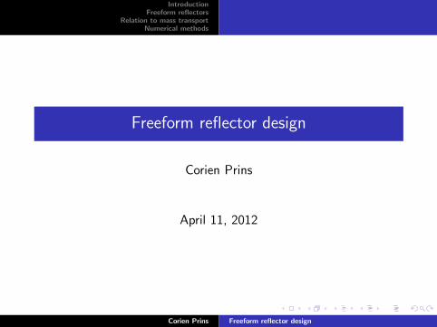
Example: car headlamp low beam




Example: car headlamp low beam

Intensity pattern of a Mercedes Low Beam




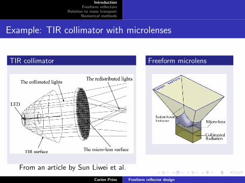
Example: TIR collimator with microlenses

TIR collimator Freeform microlens

From an article by Sun Liwei et al.




Possible applications

Square spots

Efficient car headlights

Efficient road lighting

Fancy gadgets




1 Introduction



4 Numerical methods




Inverse reflector problem

∫M(x , y) dx dy =

∫G (θ, φ) sin(θ) dθ dφ




Law of reflection

s2 = s1 − 2(s1 · n)n




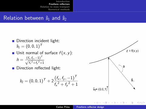
Relation between s1 and s2

Direction incident light:s1 = (0, 0, 1)T

Unit normal of surface f (x , y):

n =(fx ,fy ,−1)T√fx

2+fy2+1

Direction reflected light:

s2 = (0, 0, 1)T + 2(fx , fy ,−1)T

fx2 + fy

2 + 1




Monge-Ampere equation

Square dx dy reflected to parallellogram∣∣∣∣∣∣∂s2∂x dx × ∂s2

∂y dy∣∣∣∣∣∣

Conservation of luminous flux:

M(x , y) dx dy = G (θ, φ)

∣∣∣∣∣∣∣∣∂s2∂x dx × ∂s2∂y

dy

∣∣∣∣∣∣∣∣Basic algebra yields

∣∣∣∣∣∣∂s2∂x × ∂s2∂y

∣∣∣∣∣∣ = 4|fxy 2−fxx fyy |(fx 2+fy

2+1)2

Monge-Ampere equation: M(x ,y)G(θ,φ) = 4

|fxy 2−fxx fyy |(fx 2+fy

2+1)2




Monge-Ampere equation

Reflected angles:

θ = arccos((s2)z) = arccos

(1− 2

fx2 + fy

2 + 1

)

φ = arctan

((s2)y(s2)x

)= arctan

(fyfx

)Define: H(fx , fy ) = G

(arccos

(1− 2

fx2+fy

2+1

), arctan

(fyfx

))Finally:

∣∣fxy 2 − fxx fyy∣∣ =

(fx 2+fy2+1)

2

4M(x ,y)H(fx ,fy )




1 Introduction



4 Numerical methods




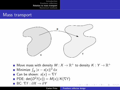
Mass transport

Move mass with density M : X → R+ to density K : Y → R+

Minimize∫X |x − s(x)|2 dx

Can be shown: s(x) = ∇fPDE: det(D2f (x)) = M(x)/K (∇f )BC: ∇f : ∂X → ∂Y




Mass transport and freeform reflector

Mass transport

Move mass from density Mto density K

PDE: det(D2f (x)) =M(x)/K (∇f )

BC: ∇f : ∂X → ∂Y

Freeform reflector

Move luminous flux fromemittance M to intensity Gor H

PDE:∣∣fxy 2 − fxx fyy

∣∣ =

(fx 2+fy2+1)

2

4M(x ,y)H(fx ,fy )

BC: ...

Remark: difficult boundary condition




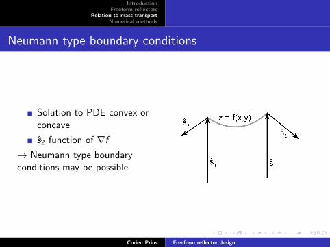
Neumann type boundary conditions

Solution to PDE convex orconcave

s2 function of ∇f→ Neumann type boundaryconditions may be possible




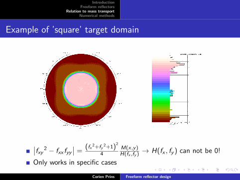
Example of ’square’ target domain

∣∣fxy 2 − fxx fyy∣∣ =

(fx 2+fy2+1)

2

4M(x ,y)H(fx ,fy )

→ H(fx , fy ) can not be 0!

Only works in specific cases




1 Introduction



4 Numerical methods




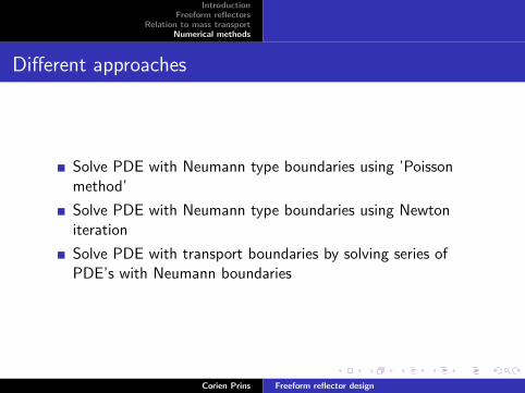
Different approaches

Solve PDE with Neumann type boundaries using ’Poissonmethod’

Solve PDE with Neumann type boundaries using Newtoniteration

Solve PDE with transport boundaries by solving series ofPDE’s with Neumann boundaries




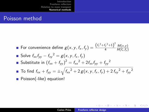
Poisson method

For convenience define g(x , y , fx , fy ) =(fx 2+fy

2+1)2

4M(x ,y)H(fx ,fy )

Solve fxx fyy − fxy2 = g(x , y , fx , fy )

Substitute in (fxx + fyy )2 = fxx2 + 2fxx fyy + fyy

2

To find fxx + fyy = ±√fxx

2 + 2 g(x , y , fx , fy ) + 2 fxy2 + fyy

2

Poisson(-like) equation!




Poisson method - example problem

Square domain: (x , y) ∈ [0, 1]× [0, 1]

M(x , y) = 1

G (θ, φ) = C ((π − θ < π/6) + 0.1)

H(fx , fy ) = G(

arccos(

1− 2fx

2+fy2+1

), arctan

(fyfx

))(fx(0, y), fx(1, y), fy (x , 0), fy (x , 1)) = (−1, 1,−1, 1)/2

Looking for convex solution

Solve on 100x100 grid




Poisson method - discretization and iteration

Standard centered differences

Square grid: fi ,j = f (xi , yj)

x-derivative: Dx f + bx → fx

y-derivative: Dy f + by → fy

xx-derivative: Dxx f + bxx → fxx

yy-derivative: Dyy f + byy → fyy

xy-derivative: Dxy f → fxy

fn+1 =fxx+fyy−f

4 − h2

4

√f2xx + f2yy + 2 f2xy + 2 g (x, y, fx , fy )

set f ← f −min(f) every iteration




Poisson method - result

After 10000 iterations, 55 secondson my laptop, max differencebetween successive iterations7 · 10−7

Result verified with Monte-Carloraytracing software




Newton iteration

Write as set of nonlinear equations N(f) = 0

Calculate Jacobi matrix J(f) = ∂N(f)∂f

The Newton method consists of the steps:

given f0

solve J(fn) sn = −N(fn)

fn+1 = fn + sn




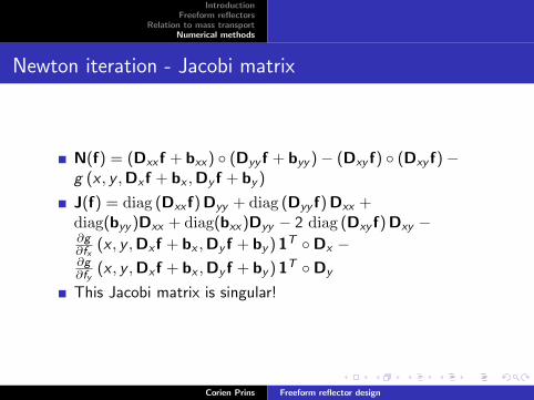
Newton iteration - Jacobi matrix

N(f) = (Dxx f + bxx) ◦ (Dyy f + byy )− (Dxy f) ◦ (Dxy f)−g (x , y ,Dx f + bx ,Dy f + by )

J(f) = diag (Dxx f) Dyy + diag (Dyy f) Dxx +diag(byy )Dxx + diag(bxx)Dyy − 2 diag (Dxy f) Dxy −∂g∂fx

(x , y ,Dx f + bx ,Dy f + by ) 1T ◦Dx −∂g∂fy

(x , y ,Dx f + bx ,Dy f + by ) 1T ◦Dy

This Jacobi matrix is singular!




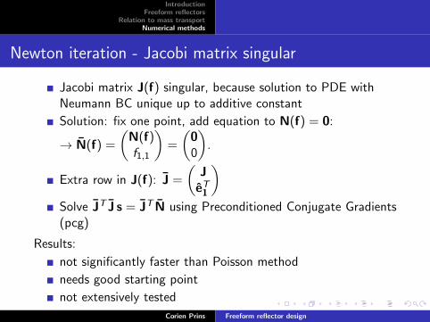
Newton iteration - Jacobi matrix singular

Jacobi matrix J(f) singular, because solution to PDE withNeumann BC unique up to additive constant

Solution: fix one point, add equation to N(f) = 0:

→ N(f) =

(N(f)f1,1

)=

(00

).

Extra row in J(f): J =

(J

eT1

)Solve JT J s = JT N using Preconditioned Conjugate Gradients(pcg)

Results:

not significantly faster than Poisson method

needs good starting point

not extensively tested




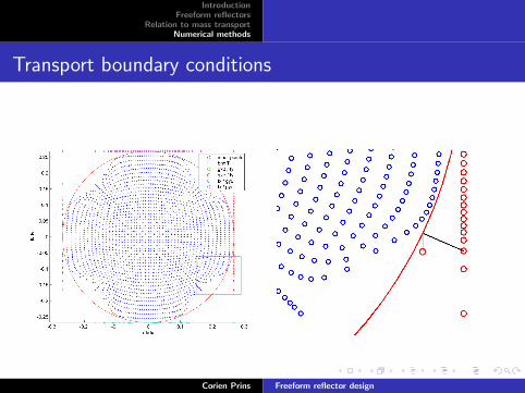
Transport boundary conditions

New method by Froese et al.

solve PDE with Neumann BC

adapt Neumann BC to real boundary

repeat procedure

complication: compatibility condition for Neumann boundaries

Method implemented but highly unstable




Transport boundary conditions




Transport boundary conditions - results




Questions?


Freeform reflector design

Documents

Transcript of Freeform reflector design