FreeFem++, 2d, 3d tools for PDE simulation - UPMC+-ANEDP.pdf · FreeFem++, 2d, 3d tools for PDE...
104
FreeFem++, 2d, 3d tools for PDE simulation F. Hecht Laboratoire Jacques-Louis Lions Universit´ e Pierre et Marie Curie Paris, France with O. Pironneau, J. Morice http://www.freefem.org mailto:[email protected] With the support of ANR (French gov.) ANR-07-CIS7-002-01 http://www.freefem.org/ff2a3/ http://www-anr-ci.cea.fr/ FreeFem++ Cours ANEDP, nov. 2010 1
Transcript of FreeFem++, 2d, 3d tools for PDE simulation - UPMC+-ANEDP.pdf · FreeFem++, 2d, 3d tools for PDE...

FreeFem++, 2d, 3d tools forPDE simulation
F. HechtLaboratoire Jacques-Louis Lions
Universite Pierre et Marie Curie
Paris, France
with O. Pironneau, J. Morice
http://www.freefem.org mailto:[email protected]
With the support of ANR (French gov.) ANR-07-CIS7-002-01
http://www.freefem.org/ff2a3/ http://www-anr-ci.cea.fr/
FreeFem++ Cours ANEDP, nov. 2010 1

PLAN
– Introduction Freefem++
– some syntaxe
– Mesh generation
– Variationnal formulation
– Poisson equation (3 formula-
tions)
– Poisson equation with matrix
– Time dependent problem
– Mesh adaptation and error indi-
cator
– Examples
– Scharwz algorithms
– Variational/Weak form (Matrix and
vector )
– mesh generation in 3d
– Coupling BEM/FEM
– Stokes variational Problem
– Navier-Stokes
– Dynamic Link example (hard)
– Conclusion / Future
http://www.freefem.org/
FreeFem++ Cours ANEDP, nov. 2010 2
Introduction
FreeFem++ is a software to solve numerically partial differential equations
(PDE) in IR2) and in IR3) with finite elements methods. We used a user
language to set and control the problem. The FreeFem++ language allows for
a quick specification of linear PDE’s, with the variational formulation of a
linear steady state problem and the user can write they own script to solve
no linear problem and time depend problem. You can solve coupled problem
or problem with moving domain or eigenvalue problem, do mesh adaptation ,
compute error indicator, etc ...
FreeFem++ is a freeware and this run on Mac, Unix and Window
architecture, in parallele with MPI.
FreeFem++ Cours ANEDP, nov. 2010 3

The main characteristics of FreeFem++ I/II (2D)
– Wide range of finite elements : linear (2d,3d) and quadratic Lagrangian
(2d,3d) elements, discontinuous P1 and Raviart-Thomas elements (2d,3d),
3d Edge element , vectorial element , mini-element( 2d, 3d), ...
– Automatic interpolation of data from a mesh to an other one, so a finite
element function is view as a function of (x, y, z) or as an array.
– Definition of the problem (complex or real value) with the variational form
with access to the vectors and the matrix if needed
– Discontinuous Galerkin formulation (only 2d to day).
FreeFem++ Cours ANEDP, nov. 2010 4

The main characteristics of FreeFem++ II/II (2D)
– Analytic description of boundaries, with specification by the user of the
intersection of boundaries in 2d.
– Automatic mesh generator, based on the Delaunay-Voronoi algorithm. (2d,3d)
– load and save Mesh, solution
– Mesh adaptation based on metric, possibly anisotropic, with optional auto-
matic computation of the metric from the Hessian of a solution.
– LU, Cholesky, Crout, CG, GMRES, UMFPack, SuperLU, MUMPS, ... sparse
linear solver ; eigenvalue and eigenvector computation with ARPACK.
– Online graphics, C++ like syntax.
– Link with other soft : modulef, emc2, medit, gnuplot, tetgen, superlu,
mumps ...
– Dynamic linking to add functonality.
– Wide range of of examples : Navier-Stokes 3d, elasticity 3d, fluid structure,
eigenvalue problem, Schwarz’ domain decomposition algorithm, residual er-
ror indicator, ...
FreeFem++ Cours ANEDP, nov. 2010 5

Element of syntaxe : Like in C++ 1/3
The key words are reserved, The basic numerical type are : int,real,complex,bool
The operator like in C exempt: ^ & |+ - * / ^ // where a^b= ab
== != < > <= >= & | // where a|b= a or b, a&b= a and b= += -= /= *=
bool: 0 <=> false , 6= 0 <=> true
// Automatic cast for numerical value : bool, int, reel, complex , sofunc heavyside = real(x>0.);
for (int i=0;i<n;i++) ... ;if ( <bool exp> ) ... ; else ...;;while ( <bool exp> ) ... ;break continue key words
// The scoop of a variable the current block : int a=1; // a blockcout << a << endl; // error the variable a not existe here.
lots of math function : exp,log, tan, ...
FreeFem++ Cours ANEDP, nov. 2010 6

Element of syntaxe 2/3
x,y,z, label, region, N.x, N.y, N.z // current coordinate, normal
int i = 0; // an integer
real a=2.5; // a reel
bool b=(a<3.);
real[int] array(10) ; // a real array of 10 value
mesh Th; mesh3 Th3; // a 2d mesh and a 3d mesh
fespace Vh(Th,P2); // a 2d finite element space;
fespace Vh3(Th3,P1); // a 3d finite element space;
Vh3 u=x; // a finite element function or array
Vh3<complex> uc = x+ 1.i *y; // complex valued FE function or array
u(.5,.6,.7); // value of FE function u at point (.5, .6, .7)
u[]; // the array associated to FE function u
u[][5]; // 6th value of the array ( numbering begin at 0 like in C)
FreeFem++ Cours ANEDP, nov. 2010 7

Element of syntaxe 3/3
fespace V3h(Th,[P2,P2,P1]);
Vh [u1,u2,p]=[x,y,z]; // a vectorial finite element function or array
// remark u1[] <==> u2[] <==> p[] same array of degree of freedom.
macro div(u,v) (dx(u)+dy(v))// EOM
macro Grad(u) [dx(u),dy(u)]// EOM
varf a([u1,u2,p],[v1,v2,q])=
int2d(Th)( Grad(u1)’*Grad(v1) +Grad(u2)’*Grad(v2)
-div(u1,u1)*q -div(v1,v2)*p)
+on(1,2)(u1=g1,u2=g2);
matrix A=a(V3h,V3h,solver=UMFPACK);
real[int] b=a(0,V3h);
p[] =A^-1*b; /* or: u1[] =A^-1*b; u2[] =A^-1*b;*/
func f=x+y; // a formal line function
func real g(int i, real a) .....; return i+a;
A = A + A’; A = A’*A // matrix operation (only one by one operation)
A = [ A,0],[0,A’]]; // Block matrix.
FreeFem++ Cours ANEDP, nov. 2010 8

Build Mesh
First a 10× 10 grid mesh of unit square ]0,1[2mesh Th1 = square(10,10); // boundary label:int[int] re=[1,1, 2,1, 3,1, 4,1] // 1 -> 1 bottom, 2 -> 1 right,
// 3->1 top, 4->1 leftTh1=change(Th1,refe=re); // boundary label is 1plot(Th1,wait=1);
second a L shape domain ]0,1[2\[12,1[2
border a(t=0,1.0)x=t; y=0; label=1;;border b(t=0,0.5)x=1; y=t; label=2;;border c(t=0,0.5)x=1-t; y=0.5;label=3;;border d(t=0.5,1)x=0.5; y=t; label=4;;border e(t=0.5,1)x=1-t; y=1; label=5;;border f(t=0.0,1)x=0; y=1-t;label=6;;plot(a(6) + b(4) + c(4) +d(4) + e(4) + f(6),wait=1); // to see the 6 bordersmesh Th2 = buildmesh (a(6) + b(4) + c(4) +d(4) + e(4) + f(6));
Get a extern meshmesh Th2("april-fish.msh");
build with emc2, bamg, modulef, etc...
FreeFem++ Cours ANEDP, nov. 2010 9

Laplace equation, weak form
Let a domain Ω with a partition of ∂Ω in Γ2,Γe.
Find u a solution in such that :
−∆u = 1 in Ω, u = 2 on Γ2,∂u
∂~n= 0 on Γe (1)
Denote Vg = v ∈ H1(Ω)/v|Γ2= g .
The Basic variationnal formulation with is : find u ∈ V2(Ω) , such that∫Ω∇u.∇v =
∫Ω
1v+∫
Γ
∂u
∂nv, ∀v ∈ V0(Ω) (2)
FreeFem++ Cours ANEDP, nov. 2010 10
Laplace equation in FreeFem++
The finite element method is just : replace Vg with a finite element space,
and the FreeFem++ code :
mesh Th("Th-hex-sph.msh");
fespace Vh(Th,P1); // define the P1 EF space
Vh u,v;
macro Grad(u) [dx(u),dy(u),dz(u)] // EOM
solve laplace(u,v,solver=CG) =
int3d(Th)( Grad(u)’*Grad(v) ) - int3d(Th) ( 1*v)
+ on(2,u=2); // int on γ2
plot(u,fill=1,wait=1,value=0,wait=1);
FreeFem++ Cours ANEDP, nov. 2010 11
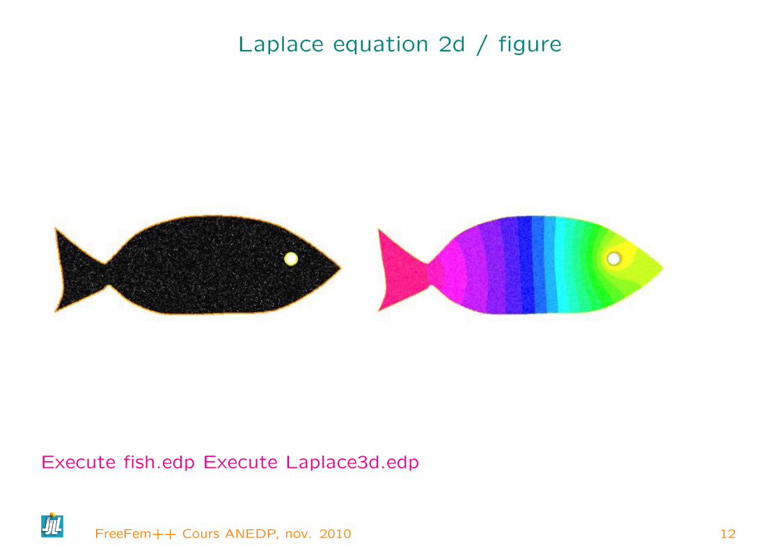
Laplace equation 2d / figure
Execute fish.edp Execute Laplace3d.edp
FreeFem++ Cours ANEDP, nov. 2010 12
The plot of the Finite Basis Function (3d plot)
load "Element_P3" // load P3 finite element
mesh Th=square(3,3); // a mesh with 2 elements
fespace Vh(Th,P3);
Vh vi=0;
for (int i=0;i<vi[].n;++i)
vi[][i]=1; // def the i+ 1th basis function
plot(vi,wait=0,cmm=" v"+i,dim=3);
vi[]=0; // undef i+ 1th basis function
Execute plot-fb.edp
FreeFem++ Cours ANEDP, nov. 2010 13

Laplace equation (mixted formulation) II/III
Now we solve −∆p = f on Ω and p = g on ∂Ω, with ~u = ∇p
so the problem becomes :
Find ~u, p a solution in a domain Ω such that :
−∇.~u = f, ~u−∇p = 0 in Ω, p = g on Γ = ∂Ω (3)
Mixted variationnal formulation
find ~u ∈ Hdiv(Ω), p ∈ L2(Ω) , such that
∫Ωq∇.~u+
∫Ωp∇.~v + ~u.~v =
∫Ω−fq +
∫Γg~v.~n, ∀(~v, q) ∈ Hdiv × L2
FreeFem++ Cours ANEDP, nov. 2010 14
Laplace equation (mixted formulation) II/III
mesh Th=square(10,10);
fespace Vh(Th,RT0); fespace Ph(Th,P0);
Vh [u1,u2],[v1,v2]; Ph p,q;
func f=1.;
func g=1;
problem laplaceMixte([u1,u2,p],[v1,v2,q],solver=LU) = //
int2d(Th)( p*q*1e-10 + u1*v1 + u2*v2
+ p*(dx(v1)+dy(v2)) + (dx(u1)+dy(u2))*q )
- int2d(Th) ( -f*q)
- int1d(Th)( (v1*N.x +v2*N.y)*g); // int on gamma
laplaceMixte; // the problem is now solved
plot([u1,u2],coef=0.1,wait=1,ps="lapRTuv.eps",value=true);
plot(p,fill=1,wait=1,ps="laRTp.eps",value=true);
Execute LaplaceRT.edp
FreeFem++ Cours ANEDP, nov. 2010 15

Laplace equation (Garlerking discutinous formulation) III/III
// solve −∆u = f on Ω and u = g on Γmacro dn(u) (N.x*dx(u)+N.y*dy(u) ) // def the normal derivative
mesh Th = square(10,10); // unite square
fespace Vh(Th,P2dc); // Discontinous P2 finite element
// if pena = 0 => Vh must be P2 otherwise we need some penalisation
real pena=0; // a parameter to add penalisation
func f=1; func g=0;
Vh u,v;
problem A(u,v,solver=UMFPACK) = //
int2d(Th)(dx(u)*dx(v)+dy(u)*dy(v) )
+ intalledges(Th)( // loop on all edge of all triangle
( jump(v)*average(dn(u)) - jump(u)*average(dn(v))
+ pena*jump(u)*jump(v) ) / nTonEdge )
- int2d(Th)(f*v)
- int1d(Th)(g*dn(v) + pena*g*v) ;
A; // solve DG
Execute LapDG2.edp
FreeFem++ Cours ANEDP, nov. 2010 16
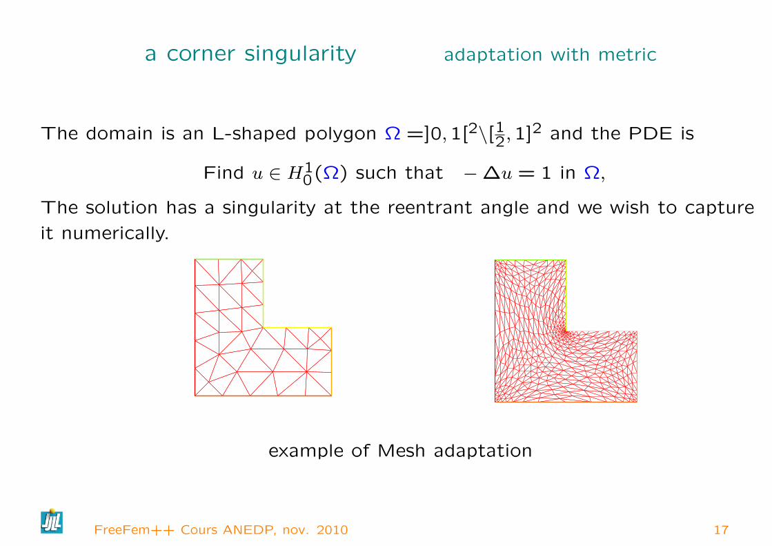
a corner singularity adaptation with metric
The domain is an L-shaped polygon Ω =]0,1[2\[12,1]2 and the PDE is
Find u ∈ H10(Ω) such that −∆u = 1 in Ω,
The solution has a singularity at the reentrant angle and we wish to capture
it numerically.
example of Mesh adaptation
FreeFem++ Cours ANEDP, nov. 2010 17

FreeFem++ corner singularity program
border a(t=0,1.0)x=t; y=0; label=1;;border b(t=0,0.5)x=1; y=t; label=2;;border c(t=0,0.5)x=1-t; y=0.5;label=3;;border d(t=0.5,1)x=0.5; y=t; label=4;;border e(t=0.5,1)x=1-t; y=1; label=5;;border f(t=0.0,1)x=0; y=1-t;label=6;;
mesh Th = buildmesh (a(6) + b(4) + c(4) +d(4) + e(4) + f(6));fespace Vh(Th,P1); Vh u,v; real error=0.01;problem Probem1(u,v,solver=CG,eps=1.0e-6) =
int2d(Th)( dx(u)*dx(v) + dy(u)*dy(v)) - int2d(Th)( v)+ on(1,2,3,4,5,6,u=0);
int i;for (i=0;i< 7;i++) Probem1; // solving the pde problem
Th=adaptmesh(Th,u,err=error); // the adaptation with Hessian of uplot(Th,wait=1); u=u; error = error/ (1000^(1./7.)) ; ;
FreeFem++ Cours ANEDP, nov. 2010 18

Matrix and vector
The 3d FreeFem++ code :
mesh3 Th("dodecaedre.mesh");
fespace Vh(Th,P13d); // define the P1 EF space
Vh u,v;
macro Grad(u) [dx(u),dy(u),dz(u)] // EOM
varf vlaplace(u,v,solver=CG) =
int3d(Th)( Grad(u)’*Grad(v) ) + int3d(Th) ( 1*v)
+ on(2,u=2); // on γ2
matrix A= vlaplace(Vh,Vh,solver=CG); // bilinear part
real[int] b=vlaplace(0,Vh); // // linear part
u[] = A^-1*b;
Execute Poisson3d.edp
FreeFem++ Cours ANEDP, nov. 2010 19
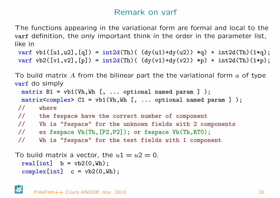
Remark on varf
The functions appearing in the variational form are formal and local to thevarf definition, the only important think in the order in the parameter list,like invarf vb1([u1,u2],[q]) = int2d(Th)( (dy(u1)+dy(u2)) *q) + int2d(Th)(1*q);
varf vb2([v1,v2],[p]) = int2d(Th)( (dy(v1)+dy(v2)) *p) + int2d(Th)(1*p);
To build matrix A from the bilinear part the the variational form a of typevarf do simplymatrix B1 = vb1(Vh,Wh [, ... optional named param ] );
matrix<complex> C1 = vb1(Vh,Wh [, ... optional named param ] );
// where
// the fespace have the correct number of component
// Vh is "fespace" for the unknown fields with 2 components
// ex fespace Vh(Th,[P2,P2]); or fespace Vh(Th,RT0);
// Wh is "fespace" for the test fields with 1 component
To build matrix a vector, the u1 = u2 = 0.real[int] b = vb2(0,Wh);
complex[int] c = vb2(0,Wh);
FreeFem++ Cours ANEDP, nov. 2010 20

The boundary condition terms
– An ”on” scalar form (for Dirichlet ) : on(1, u = g )
The meaning is for all degree of freedom i of this associated boundary,the diagonal term of the matrix aii = tgv with the terrible giant value tgv
(=1030 by default) and the right hand side b[i] = ”(Πhg)[i]” × tgv, wherethe ”(Πhg)g[i]” is the boundary node value given by the interpolation of g.
– An ”on” vectorial form (for Dirichlet ) : on(1,u1=g1,u2=g2) If you havevectorial finite element like RT0, the 2 components are coupled, and so youhave : b[i] = ”(Πh(g1, g2))[i]”× tgv, where Πh is the vectorial finite elementinterpolant.
– a linear form on Γ (for Neumann in 2d )-int1d(Th)( f*w) or -int1d(Th,3))( f*w)
– a bilinear form on Γ or Γ2 (for Robin in 2d)int1d(Th)( K*v*w) or int1d(Th,2)( K*v*w).
– a linear form on Γ (for Neumann in 3d )-int2d(Th)( f*w) or -int2d(Th,3))( f*w)
– a bilinear form on Γ or Γ2 (for Robin in 3d)int2d(Th)( K*v*w) or int2d(Th,2)( K*v*w).
FreeFem++ Cours ANEDP, nov. 2010 21

a Neumann Poisson Problem with 1D lagrange multiplier
The variationnal form is find (u, λ) ∈ Vh × R such that
∀(v, µ) ∈ Vh × R a(u, v) + b(u, µ) + b(v, λ) = l(v), where b(u, µ) =∫µudx
mesh Th=square(10,10); fespace Vh(Th,P1); // P1 FE space
int n = Vh.ndof, n1 = n+1;
func f=1+x-y; macro Grad(u) [dx(u),dy(u)] // EOM
varf va(uh,vh) = int2d(Th)( Grad(uh)’*Grad(vh) ) ;
varf vL(uh,vh) = int2d(Th)( f*vh ) ; varf vb(uh,vh)= int2d(Th)(1.*vh);
matrix A=va(Vh,Vh);
real[int] b=vL(0,Vh), B = vb(0,Vh);
real[int] bb(n1),x(n1),b1(1),l(1); b1=0;
matrix AA = [ [ A , B ] , [ B’, 0 ] ] ; bb = [ b, b1]; // blocks
set(AA,solver=UMFPACK); // set the type of linear solver.
x = AA^-1*bb; [uh[],l] = x; // solve the linear systeme
plot(uh,wait=1); // set the value
Execute Laplace-lagrange-mult.edp
FreeFem++ Cours ANEDP, nov. 2010 22

a Time depend Problem/ formulation
First, it is possible to define variational forms, and use this forms to build
matrix and vector to make very fast script (4 times faster here).
For example solve the Thermal Conduction problem of section 3.4.
The variational formulation is in L2(0, T ;H1(Ω)) ; we shall seek un satisfying
∀w ∈ V0;∫
Ω
un − un−1
δtw + κ∇un∇w) +
∫Γα(un − uue)w = 0
where V0 = w ∈ H1(Ω)/w|Γ24= 0.
FreeFem++ Cours ANEDP, nov. 2010 23
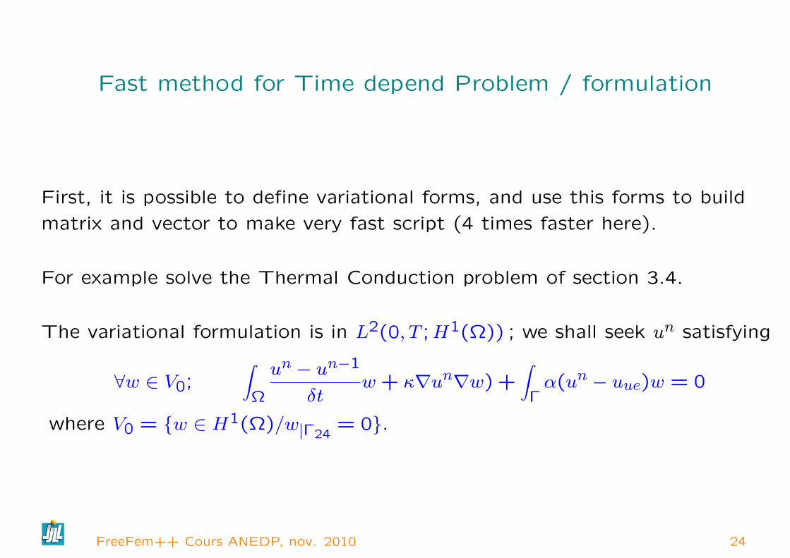
Fast method for Time depend Problem / formulation
First, it is possible to define variational forms, and use this forms to build
matrix and vector to make very fast script (4 times faster here).
For example solve the Thermal Conduction problem of section 3.4.
The variational formulation is in L2(0, T ;H1(Ω)) ; we shall seek un satisfying
∀w ∈ V0;∫
Ω
un − un−1
δtw + κ∇un∇w) +
∫Γα(un − uue)w = 0
where V0 = w ∈ H1(Ω)/w|Γ24= 0.
FreeFem++ Cours ANEDP, nov. 2010 24

Fast method for Time depend Problem algorithm
So the to code the method with the matrices A = (Aij), M = (Mij), and the
vectors un, bn, b′, b”, bcl ( notation if w is a vector then wi is a component of
the vector).
un = A−1bn, b′ = b0 +Mun−1, b” =1
εbcl, bni =
b”i if i ∈ Γ24b′i else
Where with 1ε = tgv = 1030 :
Aij =
1ε if i ∈ Γ24, and j = i∫
Ωwjwi/dt+ k(∇wj.∇wi) +
∫Γ13
αwjwi else
Mij =
1ε if i ∈ Γ24, and j = i∫
Ωwjwi/dt else
b0,i =∫
Γ13
αuuewi
bcl = u0 the initial data
FreeFem++ Cours ANEDP, nov. 2010 25

Fast The Time depend Problem/ edp
...
Vh u0=fu0,u=u0;
Create three variational formulation, and build the matrices A,M .
varf vthermic (u,v)= int2d(Th)(u*v/dt + k*(dx(u) * dx(v) + dy(u) * dy(v)))
+ int1d(Th,1,3)(alpha*u*v) + on(2,4,u=1);
varf vthermic0(u,v) = int1d(Th,1,3)(alpha*ue*v);
varf vMass (u,v)= int2d(Th)( u*v/dt) + on(2,4,u=1);
real tgv = 1e30;
A= vthermic(Vh,Vh,tgv=tgv,solver=CG);
matrix M= vMass(Vh,Vh);
FreeFem++ Cours ANEDP, nov. 2010 26

Fast The Time depend Problem/ edp
Now, to build the right hand size we need 4 vectors.
real[int] b0 = vthermic0(0,Vh); // constant part of the RHS
real[int] bcn = vthermic(0,Vh); // tgv on Dirichlet boundary node(!=0)
// we have for the node i : i ∈ Γ24 ⇔ bcn[i] 6= 0
real[int] bcl=tgv*u0[]; // the Dirichlet boundary condition part
The Fast algorithm :
for(real t=0;t<T;t+=dt)
real[int] b = b0 ; // for the RHS
b += M*u[]; // add the the time dependent part
b = bcn ? bcl : b ; // do ∀i: b[i] = bcn[i] ? bcl[i] : b[i] ;
u[] = A^-1*b;
plot(u);
FreeFem++ Cours ANEDP, nov. 2010 27

Some Idea to build meshes
The problem is to compute eigen value of a potential flow on theChesapeake bay (Thank to Mme. Sonia Garcia, smg @ usna.edu).
– Read the image in freefem, adaptmesh , trunc to
build a first mesh of the bay and finaly remove no
connected componant. We use : ξ > 0.9||ξ||∞ where
ξ is solution of
10−10ξ −∆ξ = 0 in Ω;∂ξ
∂n= 1 on Γ.
Remark, on each connect componante ω of Ω, we
have
ξ|ω ' 1010∫∂ω 1∫ω 1
.
Execute Chesapeake/Chesapeake-mesh.edp
– Solve the eigen value, on this mesh.
– Execute Chesapeake/Chesapeake-flow.edp
FreeFem++ Cours ANEDP, nov. 2010 28
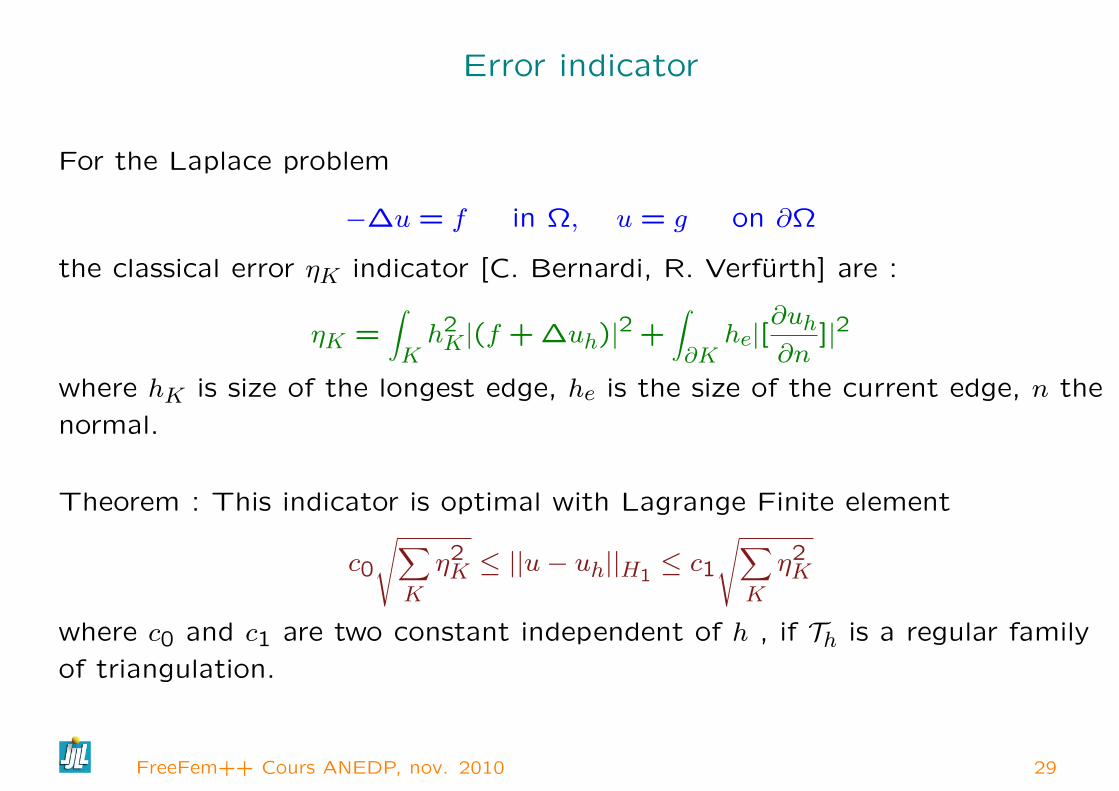
Error indicator
For the Laplace problem
−∆u = f in Ω, u = g on ∂Ω
the classical error ηK indicator [C. Bernardi, R. Verfurth] are :
ηK =∫Kh2K|(f + ∆uh)|2 +
∫∂K
he|[∂uh∂n
]|2
where hK is size of the longest edge, he is the size of the current edge, n the
normal.
Theorem : This indicator is optimal with Lagrange Finite element
c0
√∑K
η2K ≤ ||u− uh||H1
≤ c1√∑K
η2K
where c0 and c1 are two constant independent of h , if Th is a regular family
of triangulation.
FreeFem++ Cours ANEDP, nov. 2010 29

Error indicator in FreeFem++
Test on an other problem :
10−10u−∆u = x− y in Ω,∂u
∂n= 0 onΓ
remark, the 10−10u term is just to fix the constant.
We plot the density of error indicator :
ρK =ηK|K|
fespace Nh(Th,P0);
varf indicator2(uu,eta) =
intalledges(Th)( eta/lenEdge*square( jump( N.x*dx(u)+N.y*dy(u) ) ) )
+ int2d(Th)( eta*square( f+dxx(u)+dyy(u) ) );
eta[] = indicator2(0,Nh);
Execute adaptindicatorP1.edp
FreeFem++ Cours ANEDP, nov. 2010 30
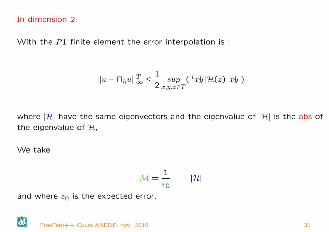
In dimension 2
With the P1 finite element the error interpolation is :
||u−Πhu||T∞ ≤1
2sup
x,y,z∈T( t ~xy |H(z)| ~xy )
where |H| have the same eigenvectors and the eigenvalue of |H| is the abs of
the eigenvalue of H,
We take
M =1
ε0|H|
and where ε0 is the expected error.
FreeFem++ Cours ANEDP, nov. 2010 31
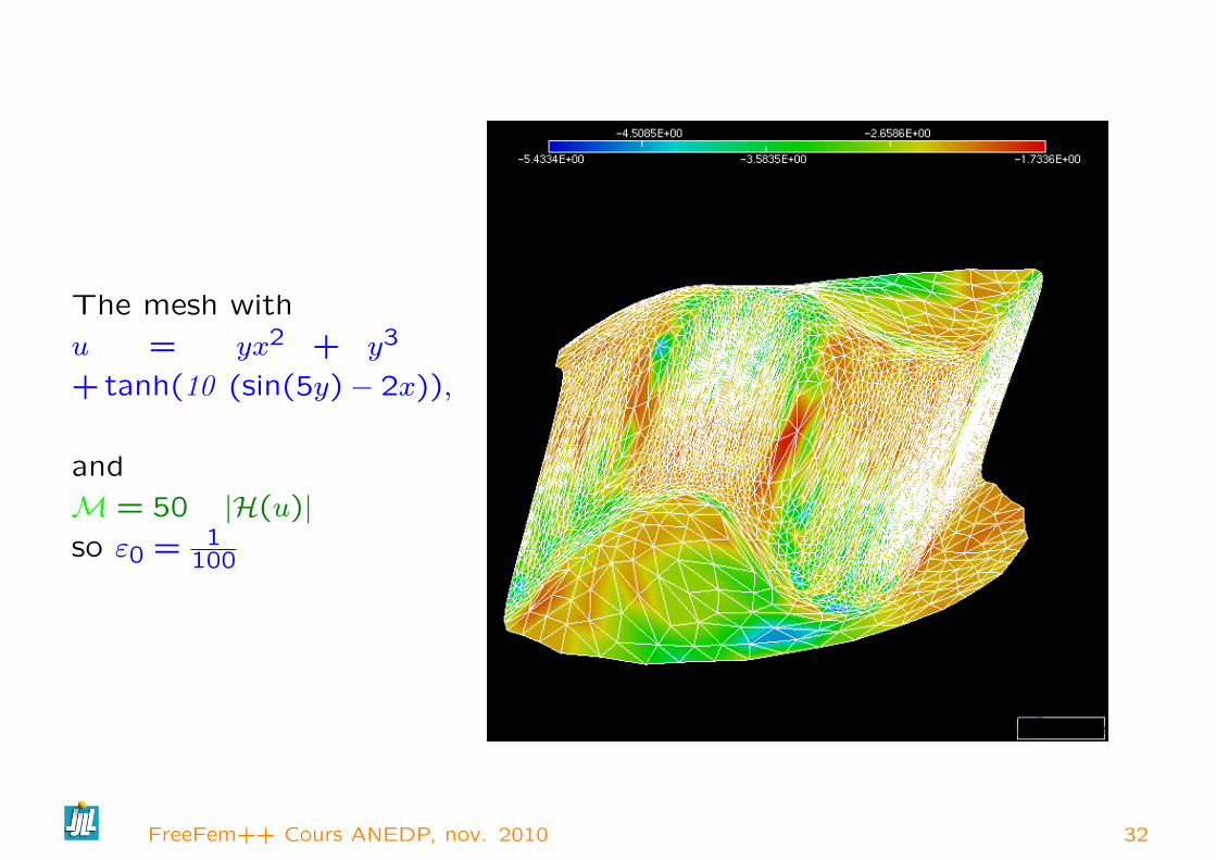
The mesh with
u = yx2 + y3
+ tanh(10 (sin(5y)− 2x)),
and
M = 50 |H(u)|so ε0 = 1
100
FreeFem++ Cours ANEDP, nov. 2010 32

Comparison : Metric and error indicator :
example of metric mesh : u = yx2 + y3 + tanh(10 (sin(5y)− 2x)) and
M = 50 |H(u)|DEMO I
Execute aaa-adp.edp
FreeFem++ Cours ANEDP, nov. 2010 33
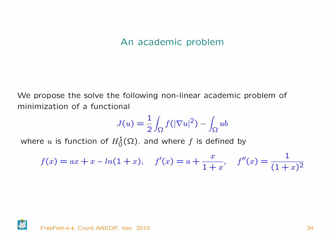
An academic problem
We propose the solve the following non-linear academic problem of
minimization of a functional
J(u) =1
2
∫Ωf(|∇u|2)−
∫Ωub
where u is function of H10(Ω). and where f is defined by
f(x) = ax+ x− ln(1 + x), f ′(x) = a+x
1 + x, f ′′(x) =
1
(1 + x)2
FreeFem++ Cours ANEDP, nov. 2010 34
FreeFem++ definition
mesh Th=square(10,10); // mesh definition of Ω
fespace Vh(Th,P1); // finite element space
fespace Ph(Th,P0); // make optimization
the definition of f , f ′, f ′′ and b
real a=0.001;
func real f(real u) return u*a+u-log(1+u);
func real df(real u) return a+u/(1+u);
func real ddf(real u) return 1/((1+u)*(1+u));
Vh b=1; // to defined b
FreeFem++ Cours ANEDP, nov. 2010 35
Newton Ralphson algorithm
Now, we solve the problem with Newton Ralphson algorithm, to solve the
Euler problem ∇J(u) = 0 the algorithm is
un+1 = un −(∇2J(un)
)−1∇J(un)
First we introduce the two variational form vdJ and vhJ to compute
respectively ∇J and ∇2J
FreeFem++ Cours ANEDP, nov. 2010 36

The variational form
Ph ddfu,dfu ; // to store f ′(|∇u|2) and 2f ′′(|∇u|2) optimization
// the variational form of evaluate dJ = ∇J// --------------------------------------
// dJ = f’()*( dx(u)*dx(vh) + dy(u)*dy(vh)
varf vdJ(uh,vh) = int2d(Th)( dfu *( dx(u)*dx(vh) + dy(u)*dy(vh) ) - b*vh)
+ on(1,2,3,4, uh=0);
// the variational form of evaluate ddJ = ∇2J
// hJ(uh,vh) = f’()*( dx(uh)*dx(vh) + dy(uh)*dy(vh)
// + f’’()( dx(u)*dx(uh) + dy(u)*dy(uh) )
// * (dx(u)*dx(vh) + dy(u)*dy(vh))
varf vhJ(uh,vh) = int2d(Th)( dfu *( dx(uh)*dx(vh) + dy(uh)*dy(vh) )
+ ddfu *(dx(u)*dx(vh) + dy(u)*dy(vh) )*(dx(u)*dx(uh) + dy(u)*dy(uh)))
+ on(1,2,3,4, uh=0);
FreeFem++ Cours ANEDP, nov. 2010 37

Newton Ralphson algorithm, next
// the Newton algorithm
Vh v,w;
u=0;
for (int i=0;i<100;i++)
dfu = df( dx(u)*dx(u) + dy(u)*dy(u) ) ; // optimization
ddfu = 2.*ddf( dx(u)*dx(u) + dy(u)*dy(u) ) ; // optimization
v[]= vdJ(0,Vh); // v = ∇J(u), v[] is the array of v
real res= v[]’*v[]; // the dot product
cout << i << " residu^2 = " << res << endl;
if( res< 1e-12) break;
matrix H= vhJ(Vh,Vh,factorize=1,solver=LU); // build and factorize
w[]=H^-1*v[]; // solve the linear system
u[] -= w[];
plot (u,wait=1,cmm="solution with Newton Ralphson");
Execute Newton.edp
FreeFem++ Cours ANEDP, nov. 2010 38

A Free Boundary problem , (phreatic water)
Let a trapezoidal domain Ω defined in FreeFem++ :
real L=10; // Width
real h=2.1; // Left height
real h1=0.35; // Right height
border a(t=0,L)x=t;y=0;label=1;; // bottom impermeable Γaborder b(t=0,h1)x=L;y=t;label=2;; // right, the source Γbborder f(t=L,0)x=t;y=t*(h1-h)/L+h;label=3;; // the free surface Γfborder d(t=h,0)x=0;y=t;label=4;; // Left impermeable Γd
int n=10;
mesh Th=buildmesh (a(L*n)+b(h1*n)+f(sqrt(L^2+(h-h1)^2)*n)+d(h*n));
plot(Th,ps="dTh.eps");
FreeFem++ Cours ANEDP, nov. 2010 39
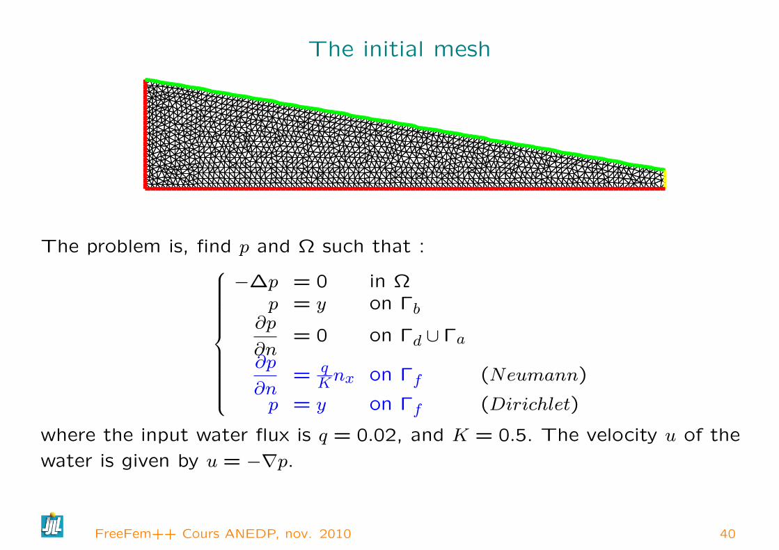
The initial mesh
The problem is, find p and Ω such that :
−∆p = 0 in Ωp = y on Γb
∂p
∂n= 0 on Γd ∪ Γa
∂p
∂n= q
Knx on Γf (Neumann)
p = y on Γf (Dirichlet)
where the input water flux is q = 0.02, and K = 0.5. The velocity u of the
water is given by u = −∇p.
FreeFem++ Cours ANEDP, nov. 2010 40

algorithm
We use the following fix point method : let be, k = 0, Ωk = Ω.
First step, we forgot the Neumann BC and we solve the problem : Find p inV = H1(Ωk), such p = y onon Γkb et on Γkf∫
Ωk∇p∇p′ = 0, ∀p′ ∈ V with p′ = 0 on Γkb ∪ Γkf
With the residual of the Neumann boundary condition we build a domaintransformation F(x, y) = [x, y − v(x)] where v is solution of : v ∈ V , such thanv = 0 on Γka (bottom)∫
Ωk∇v∇v′ =
∫Γkf
(∂p
∂n−q
Knx)v′, ∀v′ ∈ V with v′ = 0 sur Γka
remark : we can use the previous equation to evaluate∫Γk
∂p
∂nv′ = −
∫Ωk∇p∇v′
FreeFem++ Cours ANEDP, nov. 2010 41

The new domain is : Ωk+1 = F(Ωk)
Warning if is the movement is too large we can have triangle overlapping.
problem Pp(p,pp,solver=CG) = int2d(Th)( dx(p)*dx(pp)+dy(p)*dy(pp))
+ on(b,f,p=y) ;
problem Pv(v,vv,solver=CG) = int2d(Th)( dx(v)*dx(vv)+dy(v)*dy(vv))
+ on (a, v=0) + int1d(Th,f)(vv*((Q/K)*N.y- (dx(p)*N.x+dy(p)*N.y)));
while(errv>1e-6)
j++; Pp; Pv; errv=int1d(Th,f)(v*v);
coef = 1;
// Here french cooking if overlapping see the example
Th=movemesh(Th,[x,y-coef*v]); // deformation
Execute freeboundary.edp
FreeFem++ Cours ANEDP, nov. 2010 42

Eigenvalue/ Eigenvector example
The problem, Find the first λ, uλ such that :
a(uλ, v) =∫
Ω∇uλ∇v = λ
∫Ωuλv = λb(uλ, v)
the boundary condition is make with exact penalization : we put 1e30 = tgv
on the diagonal term of the lock degree of freedom. So take Dirichlet
boundary condition only with a variational form and not on b variational form
, because we compute eigenvalue of
w = A−1Bv
FreeFem++ Cours ANEDP, nov. 2010 43

Eigenvalue/ Eigenvector example code
...
fespace Vh(Th,P1);
macro Grad(u) [dx(u),dy(u),dz(u)] // EOM
varf a(u1,u2)= int3d(Th)( Grad(u1)’*Grad(u2) - sigma* u1*u2 ) +
on(1,u1=0) ;
varf b([u1],[u2]) = int3d(Th)( u1*u2 ) ; // no Boundary condition
matrix A= a(Vh,Vh,solver=UMFPACK), B= b(Vh,Vh,solver=CG,eps=1e-20);
int nev=40; // number of computed eigenvalue close to 0
real[int] ev(nev); // to store nev eigenvalue
Vh[int] eV(nev); // to store nev eigenvector
int k=EigenValue(A,B,sym=true,value=ev,vector=eV,tol=1e-10);
k=min(k,nev);
for (int i=0;i<k;i++)
plot(eV[i],cmm="Eigen 3d Vector "+i+" valeur =" +
ev[i],wait=1,value=1);
Execute Lap3dEigenValue.edp.edp
FreeFem++ Cours ANEDP, nov. 2010 44
Domain decomposition Problem
We present, three classique exemples, of domain decomposition technique :
first, Schwarz algorithm with overlapping, second Schwarz algorithm without
overlapping (also call Shur complement), and last we show to use the
conjugate gradient to solve the boundary problem of the Shur complement.
FreeFem++ Cours ANEDP, nov. 2010 45

Schwarz-overlap.edp
To solve
−∆u = f, in Ω = Ω1 ∪Ω2 u|Γ = 0
the Schwarz algorithm runs like this
−∆um+11 = f in Ω1 um+1
1 |Γ1= um2
−∆um+12 = f in Ω2 um+1
2 |Γ2= um1
where Γi is the boundary of Ωi and on the condition that Ω1 ∩Ω2 6= ∅ and
that ui are zero at iteration 1.
Here we take Ω1 to be a quadrangle, Ω2 a disk and we apply the algorithm
starting from zero.
FreeFem++ Cours ANEDP, nov. 2010 46

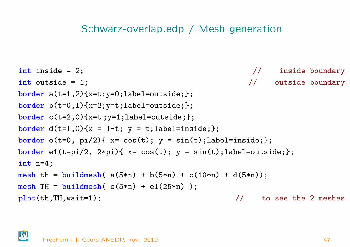
Schwarz-overlap.edp / Mesh generation
int inside = 2; // inside boundary
int outside = 1; // outside boundary
border a(t=1,2)x=t;y=0;label=outside;;
border b(t=0,1)x=2;y=t;label=outside;;
border c(t=2,0)x=t ;y=1;label=outside;;
border d(t=1,0)x = 1-t; y = t;label=inside;;
border e(t=0, pi/2) x= cos(t); y = sin(t);label=inside;;
border e1(t=pi/2, 2*pi) x= cos(t); y = sin(t);label=outside;;
int n=4;
mesh th = buildmesh( a(5*n) + b(5*n) + c(10*n) + d(5*n));
mesh TH = buildmesh( e(5*n) + e1(25*n) );
plot(th,TH,wait=1); // to see the 2 meshes
FreeFem++ Cours ANEDP, nov. 2010 47
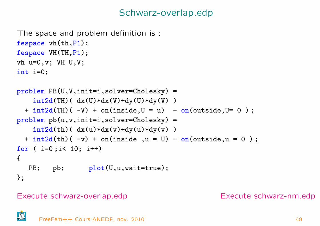
Schwarz-overlap.edp
The space and problem definition is :fespace vh(th,P1);
fespace VH(TH,P1);
vh u=0,v; VH U,V;
int i=0;
problem PB(U,V,init=i,solver=Cholesky) =
int2d(TH)( dx(U)*dx(V)+dy(U)*dy(V) )
+ int2d(TH)( -V) + on(inside,U = u) + on(outside,U= 0 ) ;
problem pb(u,v,init=i,solver=Cholesky) =
int2d(th)( dx(u)*dx(v)+dy(u)*dy(v) )
+ int2d(th)( -v) + on(inside ,u = U) + on(outside,u = 0 ) ;
for ( i=0 ;i< 10; i++)
PB; pb; plot(U,u,wait=true);
;
Execute schwarz-overlap.edp Execute schwarz-nm.edp
FreeFem++ Cours ANEDP, nov. 2010 48
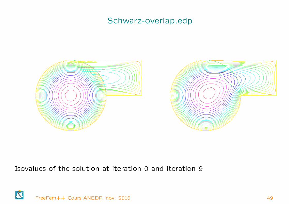
Schwarz-overlap.edp
Isovalues of the solution at iteration 0 and iteration 9
FreeFem++ Cours ANEDP, nov. 2010 49
Schwarz-no-overlap.edp
To solve
−∆u = f in Ω = Ω1 ∪Ω2 u|Γ = 0,
the Schwarz algorithm for domain decomposition without overlapping runs
like this
FreeFem++ Cours ANEDP, nov. 2010 50
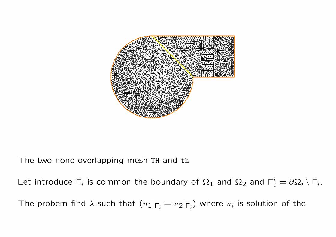
The two none overlapping mesh TH and th
Let introduce Γi is common the boundary of Ω1 and Ω2 and Γie = ∂Ωi \ Γi.
The probem find λ such that (u1|Γi = u2|Γi) where ui is solution of the

following Laplace problem :
−∆ui = f in Ωi ui|Γi = λ ui|Γie = 0
To solve this problem we just make a loop with upgradingλ with
λ = λ±(u1 − u2)
2where the sign + or − of ± is choose to have convergence.
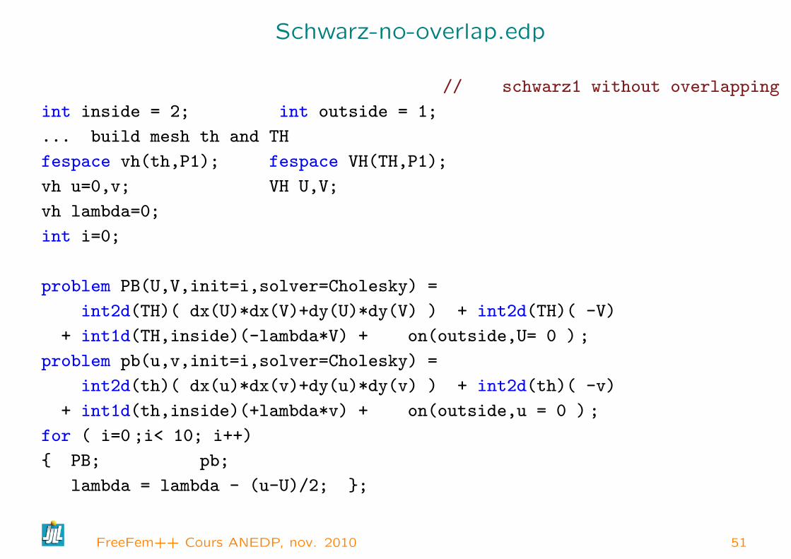
Schwarz-no-overlap.edp
// schwarz1 without overlapping
int inside = 2; int outside = 1;
... build mesh th and TH
fespace vh(th,P1); fespace VH(TH,P1);
vh u=0,v; VH U,V;
vh lambda=0;
int i=0;
problem PB(U,V,init=i,solver=Cholesky) =
int2d(TH)( dx(U)*dx(V)+dy(U)*dy(V) ) + int2d(TH)( -V)
+ int1d(TH,inside)(-lambda*V) + on(outside,U= 0 ) ;
problem pb(u,v,init=i,solver=Cholesky) =
int2d(th)( dx(u)*dx(v)+dy(u)*dy(v) ) + int2d(th)( -v)
+ int1d(th,inside)(+lambda*v) + on(outside,u = 0 ) ;
for ( i=0 ;i< 10; i++)
PB; pb;
lambda = lambda - (u-U)/2; ;
FreeFem++ Cours ANEDP, nov. 2010 51

Schwarz-no-overlap.edp
Isovalues of the solution at iteration 0 and iteration 9 without overlapping
FreeFem++ Cours ANEDP, nov. 2010 52

Schwarz-gc.edp
To solve
−∆u = f in Ω = Ω1 ∪Ω2 u|Γ = 0,
the Schwarz algorithm for domain decomposition without overlapping runs
like this
Let introduce Γi is common the boundary of Ω1 and Ω2 and Γie = ∂Ωi \ Γi.
The probem find λ such that (u1|Γi = u2|Γi) where ui is solution of the
following Laplace problem :
−∆ui = f in Ωi ui|Γi = λ ui|Γie = 0
The version of this example for Shur componant. The border problem is
solve with conjugate gradient.
FreeFem++ Cours ANEDP, nov. 2010 53

First, we construct the two domain// Schwarz without overlapping (Shur complement Neumann -> Dirichet)
real cpu=clock();int inside = 2;int outside = 1;
border Gamma1(t=1,2)x=t;y=0;label=outside;;border Gamma2(t=0,1)x=2;y=t;label=outside;;border Gamma3(t=2,0)x=t ;y=1;label=outside;;
border GammaInside(t=1,0)x = 1-t; y = t;label=inside;;
border GammaArc(t=pi/2, 2*pi) x= cos(t); y = sin(t);label=outside;;int n=4;
// build the mesh of Ω1 and Ω2
mesh Th1 = buildmesh( Gamma1(5*n) + Gamma2(5*n) + GammaInside(5*n) + Gamma3(5*n));mesh Th2 = buildmesh ( GammaInside(-5*n) + GammaArc(25*n) );plot(Th1,Th2);
// defined the 2 FE spacefespace Vh1(Th1,P1), Vh2(Th2,P1);

Schwarz-gc.edp, next
Remark, to day is not possible to defined a function just on a border, so the
λ function is defined on the all domain Ω1 by :
Vh1 lambda=0; // take λ ∈ Vh1
The two Laplace problem :
Vh1 u1,v1; Vh2 u2,v2;
int i=0; // for factorization optimization
problem Pb2(u2,v2,init=i,solver=Cholesky) =
int2d(Th2)( dx(u2)*dx(v2)+dy(u2)*dy(v2) )
+ int2d(Th2)( -v2)
+ int1d(Th2,inside)(-lambda*v2) + on(outside,u2= 0 ) ;
problem Pb1(u1,v1,init=i,solver=Cholesky) =
int2d(Th1)( dx(u1)*dx(v1)+dy(u1)*dy(v1) )
+ int2d(Th1)( -v1)
+ int1d(Th1,inside)(+lambda*v1) + on(outside,u1 = 0 ) ;
FreeFem++ Cours ANEDP, nov. 2010 54

Schwarz-gc.edp, next I
Now, we define a border matrix , because the λ function is none zero insidethe domain Ω1 :varf b(u2,v2,solver=CG) =int1d(Th1,inside)(u2*v2);
matrix B= b(Vh1,Vh1,solver=CG);
The boundary problem function,
λ −→∫
Γi(u1 − u2)v1
func real[int] BoundaryProblem(real[int] &l)
lambda[]=l; // make FE function form l
Pb1; Pb2;
i++; // no refactorization i !=0
v1=-(u1-u2);
lambda[]=B*v1[];
return lambda[] ;
;
FreeFem++ Cours ANEDP, nov. 2010 55

Schwarz-gc.edp, next II
Remark, the difference between the two notations v1 and v1[] is : v1 is the
finite element function and v1[] is the vector in the canonical basis of the
finite element function v1 .
Vh1 p=0,q=0;
// solve the problem with Conjugue Gradient
LinearCG(BoundaryProblem,p[],eps=1.e-6,nbiter=100);
// compute the final solution, because CG works with increment
BoundaryProblem(p[]); // solve again to have right u1,u2
cout << " -- CPU time schwarz-gc:" << clock()-cpu << endl;
plot(u1,u2); // plot
FreeFem++ Cours ANEDP, nov. 2010 56

A cube
load "msh3" // buildlayer
int nn=10;
int[int] rup=[0,2], rdown=[0,1], rmid=[1,1,2,1,3,1,4,1],rtet[0,0];
real zmin=0,zmax=1;
mesh3 Th=buildlayers(square(nn,nn),nn,
zbound=[zmin,zmax],
reftet=rtet,
reffacemid=rmid,
reffaceup = rup,
reffacelow = rdown);
savemesh(Th,"c10x10x10.mesh");
exec("medit c10x10x10;rm c10x10x10.mesh");
Execute Cube.edp
FreeFem++ Cours ANEDP, nov. 2010 57
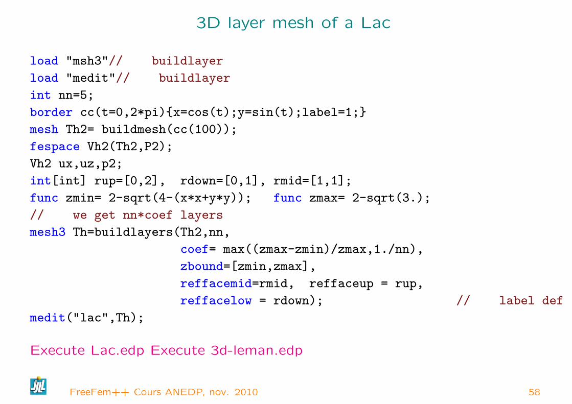
3D layer mesh of a Lac
load "msh3"// buildlayer
load "medit"// buildlayer
int nn=5;
border cc(t=0,2*pi)x=cos(t);y=sin(t);label=1;
mesh Th2= buildmesh(cc(100));
fespace Vh2(Th2,P2);
Vh2 ux,uz,p2;
int[int] rup=[0,2], rdown=[0,1], rmid=[1,1];
func zmin= 2-sqrt(4-(x*x+y*y)); func zmax= 2-sqrt(3.);
// we get nn*coef layers
mesh3 Th=buildlayers(Th2,nn,
coef= max((zmax-zmin)/zmax,1./nn),
zbound=[zmin,zmax],
reffacemid=rmid, reffaceup = rup,
reffacelow = rdown); // label def
medit("lac",Th);
Execute Lac.edp Execute 3d-leman.edp
FreeFem++ Cours ANEDP, nov. 2010 58
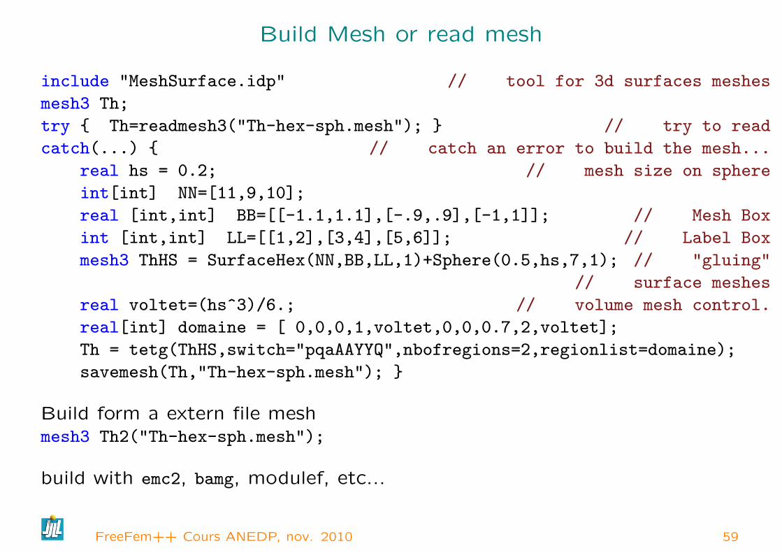
Build Mesh or read mesh
include "MeshSurface.idp" // tool for 3d surfaces meshes
mesh3 Th;
try Th=readmesh3("Th-hex-sph.mesh"); // try to read
catch(...) // catch an error to build the mesh...
real hs = 0.2; // mesh size on sphere
int[int] NN=[11,9,10];
real [int,int] BB=[[-1.1,1.1],[-.9,.9],[-1,1]]; // Mesh Box
int [int,int] LL=[[1,2],[3,4],[5,6]]; // Label Box
mesh3 ThHS = SurfaceHex(NN,BB,LL,1)+Sphere(0.5,hs,7,1); // "gluing"
// surface meshes
real voltet=(hs^3)/6.; // volume mesh control.
real[int] domaine = [ 0,0,0,1,voltet,0,0,0.7,2,voltet];
Th = tetg(ThHS,switch="pqaAAYYQ",nbofregions=2,regionlist=domaine);
savemesh(Th,"Th-hex-sph.mesh");
Build form a extern file meshmesh3 Th2("Th-hex-sph.mesh");
build with emc2, bamg, modulef, etc...
FreeFem++ Cours ANEDP, nov. 2010 59
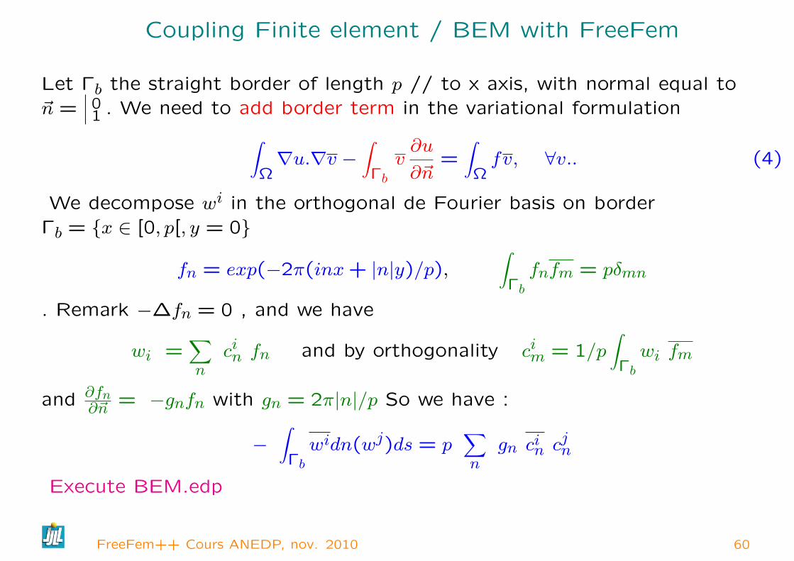
Coupling Finite element / BEM with FreeFem
Let Γb the straight border of length p // to x axis, with normal equal to~n =
∣∣∣ 01 . We need to add border term in the variational formulation∫
Ω∇u.∇v −
∫Γbv∂u
∂~n=∫
Ωfv, ∀v.. (4)
We decompose wi in the orthogonal de Fourier basis on borderΓb = x ∈ [0, p[, y = 0
fn = exp(−2π(inx+ |n|y)/p),∫
Γbfnfm = pδmn
. Remark −∆fn = 0 , and we have
wi =∑n
cin fn and by orthogonality cim = 1/p∫
Γbwi fm
and ∂fn∂~n = −gnfn with gn = 2π|n|/p So we have :
−∫
Γbwidn(wj)ds = p
∑n
gn cin cjn
Execute BEM.edp
FreeFem++ Cours ANEDP, nov. 2010 60
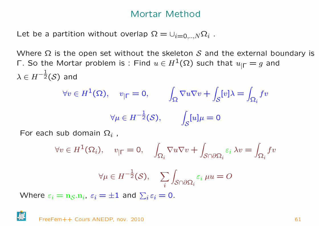
Mortar Method
Let be a partition without overlap Ω = ∪i=0,..,NΩi .
Where Ω is the open set without the skeleton S and the external boundary isΓ. So the Mortar problem is : Find u ∈ H1(Ω) such that u|Γ = g and
λ ∈ H−12(S) and
∀v ∈ H1(Ω), v|Γ = 0,∫
Ω∇u∇v +
∫S
[v]λ =∫
Ωi
fv
∀µ ∈ H−12(S),
∫S
[u]µ = 0
For each sub domain Ωi ,
∀v ∈ H1(Ωi), v|Γ = 0,∫
Ωi
∇u∇v +∫S∩∂Ωi
εi λv =∫
Ωi
fv
∀µ ∈ H−12(S),
∑i
∫S∩∂Ωi
εi µu = O
Where εi = nS.ni, εi = ±1 and∑i εi = 0.
FreeFem++ Cours ANEDP, nov. 2010 61

Mortar Method Precond
J ′(λ)(µ) = −∫S
[uλ]µ = 0 ∀µ
where uλ if solution of
∀v ∈ H1(Ωi), v|Γ = 0,∫
Ωi
∇uλ∇v +∫S∩∂Ωi
εi λv =∫
Ωi
fv
For each sub domain Ωi ,
∀v ∈ H1(Ωi), v|Γ = 0,∫
Ωi
∇u∇v +∫S∩∂Ωi
εi λv =∫
Ωi
fv
∀µ ∈ H−12(S),
∑i
∫S∩∂Ωi
εi µu = O
Where εi = nS.ni, εi = ±1 and∑i εi = 0.
FreeFem++ Cours ANEDP, nov. 2010 62
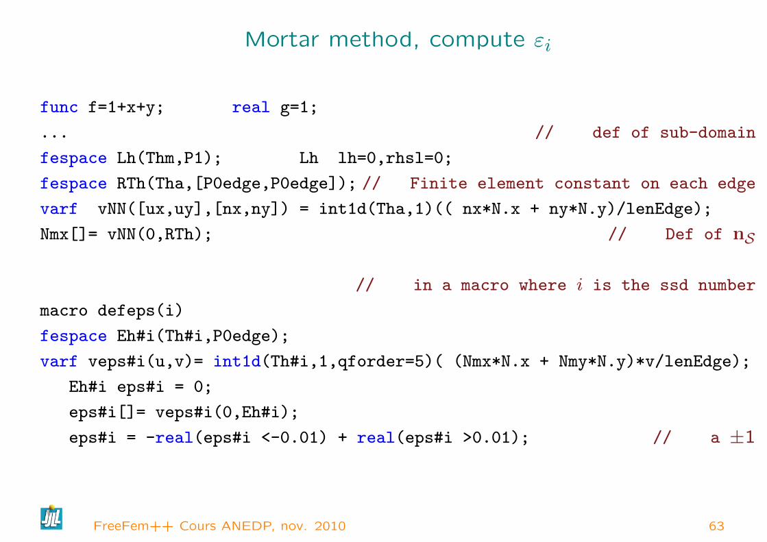
Mortar method, compute εi
func f=1+x+y; real g=1;
... // def of sub-domain
fespace Lh(Thm,P1); Lh lh=0,rhsl=0;
fespace RTh(Tha,[P0edge,P0edge]); // Finite element constant on each edge
varf vNN([ux,uy],[nx,ny]) = int1d(Tha,1)(( nx*N.x + ny*N.y)/lenEdge);
Nmx[]= vNN(0,RTh); // Def of nS
// in a macro where i is the ssd number
macro defeps(i)
fespace Eh#i(Th#i,P0edge);
varf veps#i(u,v)= int1d(Th#i,1,qforder=5)( (Nmx*N.x + Nmy*N.y)*v/lenEdge);
Eh#i eps#i = 0;
eps#i[]= veps#i(0,Eh#i);
eps#i = -real(eps#i <-0.01) + real(eps#i >0.01); // a ±1
FreeFem++ Cours ANEDP, nov. 2010 63

Mortar method
macro defspace(i)
cout << " Domaine " << i<< " --------" << endl;
fespace Vh#i(Th#i,P1);
Vh#i u#i; Vh#i rhs#i;
defeps(i)
varf vLapM#i([u#i],[v#i]) =
int2d(Th#i)( Grad(u#i)’*Grad(v#i) ) + int2d(Th#i) (f*v#i)
+ on(labext,u#i=g) ;
varf cc#i([l],[u]) = int1d( Thmm,1)(l*u*eps#i);
matrix C#i = cc#i(Lh,Vh#i);
matrix A#i = vLapM#i(Vh#i,Vh#i,solver=GMRES);
rhs#i[]=vLapM#i(0,Vh#i); // End of macro defspace(i)
defspace(0) defspace(1) defspace(2) defspace(3)
FreeFem++ Cours ANEDP, nov. 2010 64
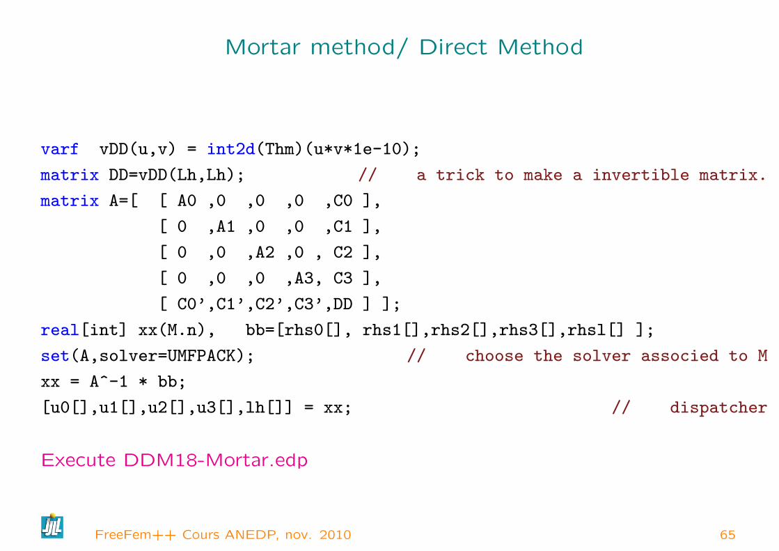
Mortar method/ Direct Method
varf vDD(u,v) = int2d(Thm)(u*v*1e-10);
matrix DD=vDD(Lh,Lh); // a trick to make a invertible matrix.
matrix A=[ [ A0 ,0 ,0 ,0 ,C0 ],
[ 0 ,A1 ,0 ,0 ,C1 ],
[ 0 ,0 ,A2 ,0 , C2 ],
[ 0 ,0 ,0 ,A3, C3 ],
[ C0’,C1’,C2’,C3’,DD ] ];
real[int] xx(M.n), bb=[rhs0[], rhs1[],rhs2[],rhs3[],rhsl[] ];
set(A,solver=UMFPACK); // choose the solver associed to M
xx = A^-1 * bb;
[u0[],u1[],u2[],u3[],lh[]] = xx; // dispatcher
Execute DDM18-Mortar.edp
FreeFem++ Cours ANEDP, nov. 2010 65

Mortar method/ GC method
func real[int] SkPb(real[int] &l)
int verb=verbosity; verbosity=0; itera++;
v0[] = rhs0[]; v0[]+= C0* l; u0[] = A0^-1*v0[];
v1[] = rhs1[]; v1[]+= C1* l; u1[] = A1^-1*v1[];
v2[] = rhs2[]; v2[]+= C2* l; u2[] = A2^-1*v2[];
v3[] = rhs3[]; v3[]+= C3* l; u3[] = A3^-1*v3[];
l = C1’*u1[]; l += C0’*u0[]; l += C2’*u2[];
l += C3’*u3[]; l= lbc ? lbc0: l;
verbosity=verb;
return l ; ;
verbosity=100; lh[]=0;
LinearCG(SkPb,lh[],eps=1.e-2,nbiter=30);
FreeFem++ Cours ANEDP, nov. 2010 66
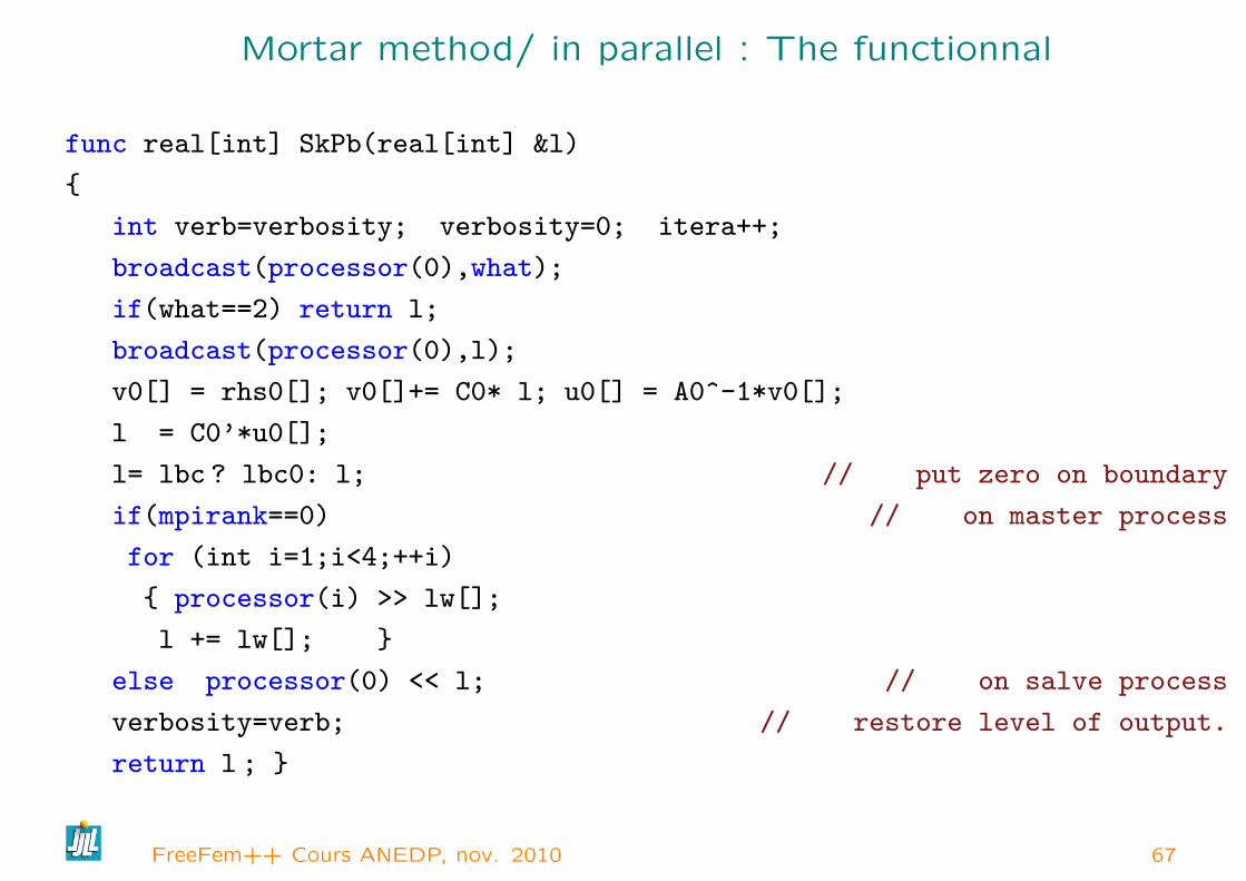
Mortar method/ in parallel : The functionnal
func real[int] SkPb(real[int] &l)
int verb=verbosity; verbosity=0; itera++;
broadcast(processor(0),what);
if(what==2) return l;
broadcast(processor(0),l);
v0[] = rhs0[]; v0[]+= C0* l; u0[] = A0^-1*v0[];
l = C0’*u0[];
l= lbc ? lbc0: l; // put zero on boundary
if(mpirank==0) // on master process
for (int i=1;i<4;++i)
processor(i) >> lw[];
l += lw[];
else processor(0) << l; // on salve process
verbosity=verb; // restore level of output.
return l ;
FreeFem++ Cours ANEDP, nov. 2010 67

Mortar method/ CG in parallel
what=1;verbosity=100;if(mpirank==0) // on master processLinearCG(SkPb,lh[],eps=1.e-3,nbiter=20); // future withprocess=[0,1,2,3]what=2; SkPb(lh[]);else // on slave processwhile(what==1)
SkPb(lh[]);
Execute DDM18-mortar-mpi.edp
FreeFem++ Cours ANEDP, nov. 2010 68

Dynamics Load facility
Or How to add your C++ function in FreeFem++.
First, like in cooking, the first true difficulty is how to use the kitchen.
I suppose you can compile the first example for the examples++-load
numermac11:FH-Seville hecht# ff-c++ myppm2rnm.cppexport MACOSX_DEPLOYMENT_TARGET=10.3g++ -c -DNDEBUG -O3 -O3 -march=pentium4 -DDRAWING -DBAMG_LONG_LONG -DNCHECKPTR-I/usr/X11/include -I/usr/local/lib/ff++/3.4/include ’myppm2rnm.cpp’g++ -bundle -undefined dynamic_lookup -DNDEBUG -O3 -O3 -march=pentium4 -DDRAWING-DBAMG_LONG_LONG -DNCHECKPTR -I/usr/X11/include ’myppm2rnm.o’ -o myppm2rnm.dylib
add tools to read pgm image
FreeFem++ Cours ANEDP, nov. 2010 69

The interesting code
#include "ff++.hpp"typedef KNM<double> * pRnm; // the freefem++ real[int,int] array variable typetypedef KN<double> * pRn; // the freefem++ real[int] array variable typetypedef string ** string; // the freefem++ string variable type
pRnm read_image( pRnm const & a,const pstring & b); // the function to read imagepRn seta( pRn const & a,const pRnm & b) // the function to set 2d array from 1d array *a=*b;KN_<double> aa=*a;return a;
class Init public: Init(); ; // C++ trick to call a method at load timeInit init; // a global variable to inforce the initialisation by c++Init::Init() // the like with FreeFem++ s// add ff++ operator "<-" constructor of real[int,int] form a stringTheOperators->Add("<-",
new OneOperator2_<KNM<double> *,KNM<double> *,string*>(&read_image));// add ff++ an affection "=" of real[int] form a real[int,int]TheOperators->Add("=",
new OneOperator2_<KN<double> *,KN<double> *,KNM<double>* >(seta));
Remark, TheOperators is the ff++ variable to store all world operator, Global
is to store function.
FreeFem++ Cours ANEDP, nov. 2010 70
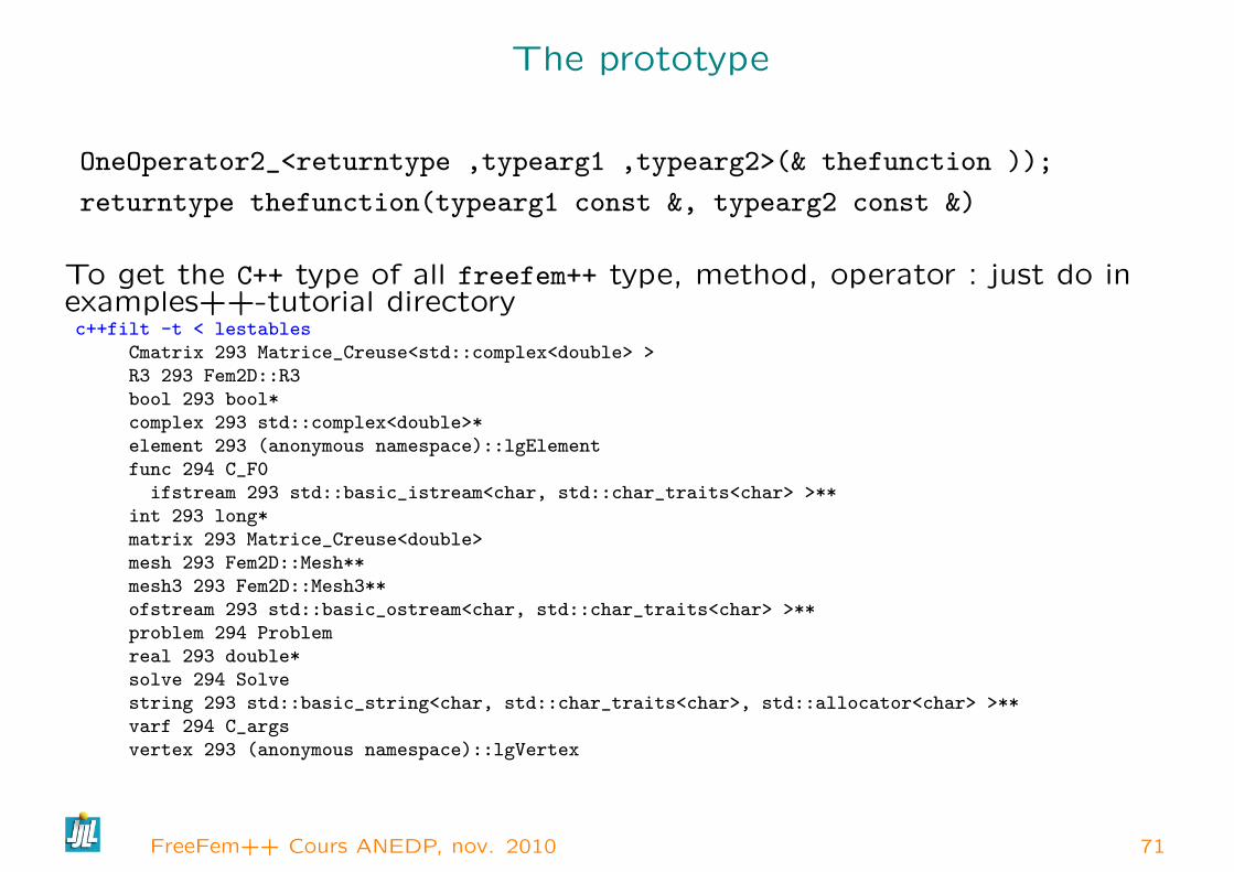
The prototype
OneOperator2_<returntype ,typearg1 ,typearg2>(& thefunction ));
returntype thefunction(typearg1 const &, typearg2 const &)
To get the C++ type of all freefem++ type, method, operator : just do inexamples++-tutorial directoryc++filt -t < lestables
Cmatrix 293 Matrice_Creuse<std::complex<double> >R3 293 Fem2D::R3bool 293 bool*complex 293 std::complex<double>*element 293 (anonymous namespace)::lgElementfunc 294 C_F0ifstream 293 std::basic_istream<char, std::char_traits<char> >**
int 293 long*matrix 293 Matrice_Creuse<double>mesh 293 Fem2D::Mesh**mesh3 293 Fem2D::Mesh3**ofstream 293 std::basic_ostream<char, std::char_traits<char> >**problem 294 Problemreal 293 double*solve 294 Solvestring 293 std::basic_string<char, std::char_traits<char>, std::allocator<char> >**varf 294 C_argsvertex 293 (anonymous namespace)::lgVertex
FreeFem++ Cours ANEDP, nov. 2010 71

FreeFem++ Triangle/Tet capabylity
// soit T un Element de sommets A,B,C ∈ R2
// ------------------------------------Element::nv ; // nombre de sommets d’un triangle (ici 3)const Element::Vertex & V = T[i]; // le sommet i de T (i ∈ 0,1,2double a = T.mesure() ; // mesure de TRd AB = T.Edge(2); // "vecteur arete" de l’areteRd hC = T.H(2) ; // gradient de la fonction de base associe au sommet 2R l = T.lenEdge(i); // longueur de l’arete opposee au sommet i(Label) T ; // la reference du triangle TR2 G(T(R2(1./3,1./3))); // le barycentre de T in 3d
FreeFem++ Cours ANEDP, nov. 2010 72
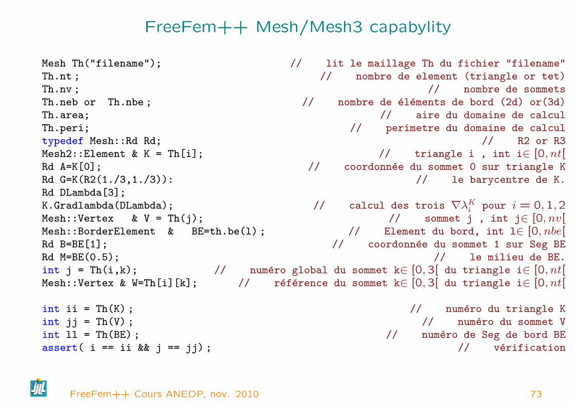
FreeFem++ Mesh/Mesh3 capabylity
Mesh Th("filename"); // lit le maillage Th du fichier "filename"Th.nt ; // nombre de element (triangle or tet)Th.nv ; // nombre de sommetsTh.neb or Th.nbe ; // nombre de elements de bord (2d) or(3d)Th.area; // aire du domaine de calculTh.peri; // perimetre du domaine de calcultypedef Mesh::Rd Rd; // R2 or R3Mesh2::Element & K = Th[i]; // triangle i , int i∈ [0, nt[Rd A=K[0]; // coordonnee du sommet 0 sur triangle KRd G=K(R2(1./3,1./3)): // le barycentre de K.Rd DLambda[3];K.Gradlambda(DLambda); // calcul des trois ∇λKi pour i = 0,1,2Mesh::Vertex & V = Th(j); // sommet j , int j∈ [0, nv[Mesh::BorderElement & BE=th.be(l) ; // Element du bord, int l∈ [0, nbe[Rd B=BE[1]; // coordonnee du sommet 1 sur Seg BERd M=BE(0.5); // le milieu de BE.int j = Th(i,k); // numero global du sommet k∈ [0,3[ du triangle i∈ [0, nt[Mesh::Vertex & W=Th[i][k]; // reference du sommet k∈ [0,3[ du triangle i∈ [0, nt[
int ii = Th(K) ; // numero du triangle Kint jj = Th(V) ; // numero du sommet Vint ll = Th(BE) ; // numero de Seg de bord BEassert( i == ii && j == jj) ; // verification
FreeFem++ Cours ANEDP, nov. 2010 73
Some Example (from the archive)
– Execute BlackScholes2D.edp
– Execute Poisson-mesh-adap.edp
– Execute Micro-wave.edp
– Execute wafer-heating-laser-axi.edp
– Execute nl-elast-neo-Hookean.edp
– Execute Stokes-eigen.edp
– Execute fluid-Struct-with-Adapt.edp
– Execute optim-control.edp
– Execute VI-2-menbrane-adap.edp
FreeFem++ Cours ANEDP, nov. 2010 74

An exercice in FreeFem++
The geometrical problem : Find a function u : C1(Ω) 7→ R where u is given onΓ = ∂Ω, (e.i. u|Γ = g) such that the area of the surface S parametrize by(x, y) ∈ Ω 7→ (x, y, u(x, y)) is minimal.
So the problem is arg minJ(u) where
J(u) =∫∫
Ω
∣∣∣∣∣∣∣∣∣∣∣∣∣∣ 1
0∂xu
× 0
1∂yu
∣∣∣∣∣∣∣∣∣∣∣∣∣∣2
dxdy =∫∫
Ω
√1 +∇u.∇u dxdy
So the Euler equation associated to the minimisaton is :
∀v/v|Γ = 0 : DJ(u)(v) =∫∫
Ω
∇u.∇v√1 +∇u.∇u
= 0
and the gradient associated to the scalar product X is solution of :
∀v/v|Γ = 0 : (∇J(u), v)X = DJ(u)(v)
So find the solution for Ω =]0, π[2[ and g(x, y) = cos(2 ∗ x) ∗ cos(2 ∗ y). byusing the Non Linear Conjugate gradient NLCG like in the example : algo.edp
in examples++-tutorial.
FreeFem++ Cours ANEDP, nov. 2010 75

Tools
Example of use of NLCG function :
Vh u; // the finite to store the current valuefunc real J(real[int] & xx) // the functionnal to mininized real s=0;u[]=xx; // add code to copy xx array of finite element function... // /return s;
Use the varf tools to build the vector DJ(u)(wi)i.func real[int] DJ(real[int] &xx) // the grad of functionnal u[]=xx; // add code to copy xx array of finite element function.... //return xx; ; // return of an existing variable ok
...u=g;NLCG(DJ,u[],eps=1.e-6,nbiter=20);
To see the 3D plot of the surface
plot(u,dim=3,wait=1);
FreeFem++ Cours ANEDP, nov. 2010 76

The C++ kernel / Dehli, (1992 ) (Idea, I)
My early step in C++
typedef double R;class Cvirt public: virtual R operator()(R ) const =0;;
class Cfonc : public Cvirt public:R (*f)(R); // a function CR operator()(R x) const return (*f)(x);Cfonc( R (*ff)(R)) : f(ff) ;
class Coper : public Cvirt public:const Cvirt *g, *d; // the 2 functionsR (*op)(R,R); // l’operationR operator()(R x) const return (*op)((*g)(x),(*d)(x));Coper( R (*opp)(R,R), const Cvirt *gg, const Cvirt *dd): op(opp),g(gg),d(dd)
~Coper()delete g,delete d; ;
static R Add(R a,R b) return a+b; static R Sub(R a,R b) return a-b;static R Mul(R a,R b) return a*b; static R Div(R a,R b) return a/b;static R Pow(R a,R b) return pow(a,b);
FreeFem++ Cours ANEDP, nov. 2010 77
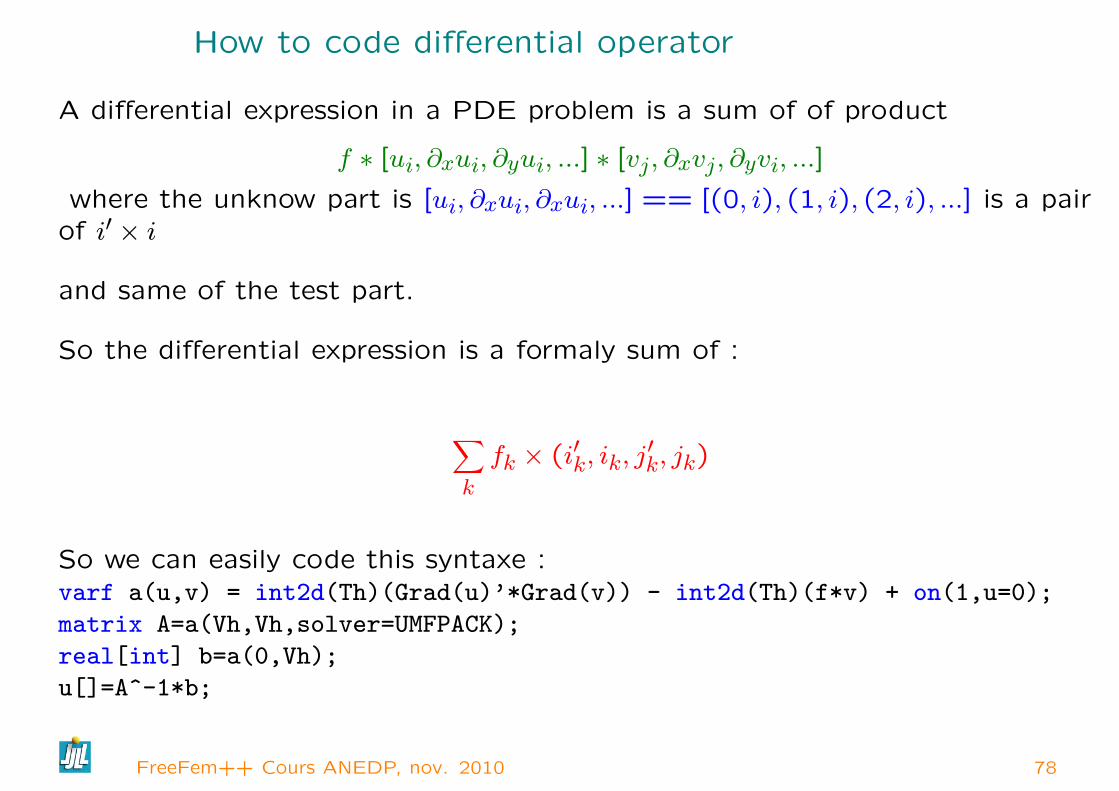
How to code differential operator (Idea, II)
A differential expression in a PDE problem is a sum of of product
f ∗ [ui, ∂xui, ∂yui, ...] ∗ [vj, ∂xvj, ∂yvi, ...]
where the unknow part is [ui, ∂xui, ∂xui, ...] == [(0, i), (1, i), (2, i), ...] is a pairof i′ × i
and same of the test part.
So the differential expression is a formaly sum of :
∑k
fk × (i′k, ik, j′k, jk)
So we can easily code this syntaxe :varf a(u,v) = int2d(Th)(Grad(u)’*Grad(v)) - int2d(Th)(f*v) + on(1,u=0);
matrix A=a(Vh,Vh,solver=UMFPACK);
real[int] b=a(0,Vh);
u[]=A^-1*b;
FreeFem++ Cours ANEDP, nov. 2010 78
Au boulot !
FreeFem++ Cours ANEDP, nov. 2010 79
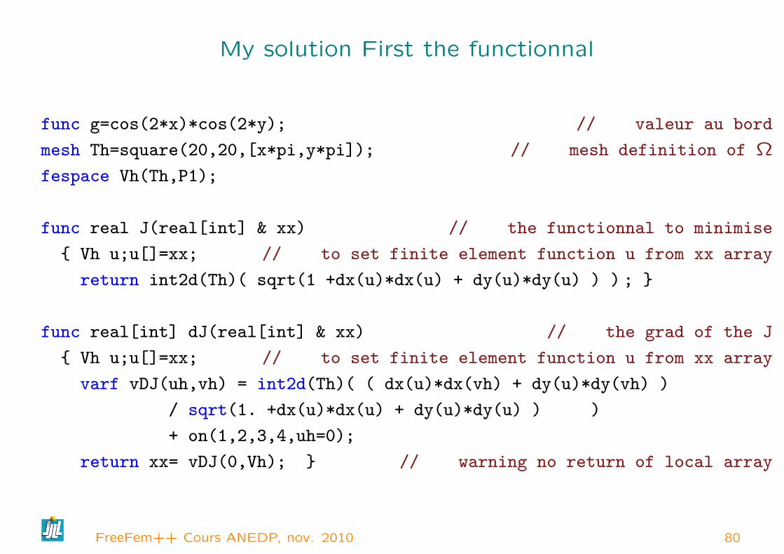
My solution First the functionnal
func g=cos(2*x)*cos(2*y); // valeur au bord
mesh Th=square(20,20,[x*pi,y*pi]); // mesh definition of Ω
fespace Vh(Th,P1);
func real J(real[int] & xx) // the functionnal to minimise
Vh u;u[]=xx; // to set finite element function u from xx array
return int2d(Th)( sqrt(1 +dx(u)*dx(u) + dy(u)*dy(u) ) ) ;
func real[int] dJ(real[int] & xx) // the grad of the J
Vh u;u[]=xx; // to set finite element function u from xx array
varf vDJ(uh,vh) = int2d(Th)( ( dx(u)*dx(vh) + dy(u)*dy(vh) )
/ sqrt(1. +dx(u)*dx(u) + dy(u)*dy(u) ) )
+ on(1,2,3,4,uh=0);
return xx= vDJ(0,Vh); // warning no return of local array
FreeFem++ Cours ANEDP, nov. 2010 80
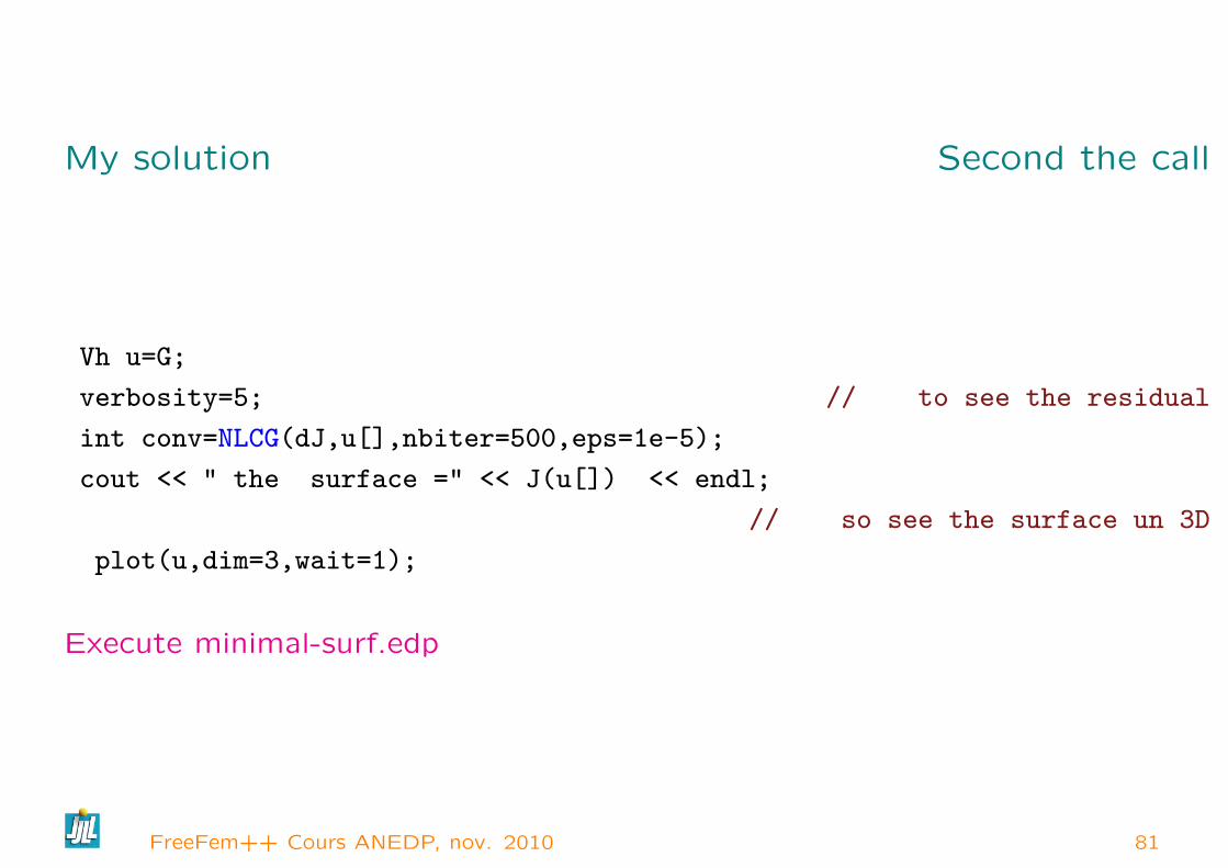
My solution Second the call
Vh u=G;
verbosity=5; // to see the residual
int conv=NLCG(dJ,u[],nbiter=500,eps=1e-5);
cout << " the surface =" << J(u[]) << endl;
// so see the surface un 3D
plot(u,dim=3,wait=1);
Execute minimal-surf.edp
FreeFem++ Cours ANEDP, nov. 2010 81

An exercice in FreeFem++, next
The algorithm is to slow, To speed up the converge after some few iteration
of NLCG, you can use a Newtow method and make also mesh adaptation.
The Newton algorithm to solve F (u) = 0 is make the loop :
un+1 = un − wn; with DF (un)(wn) = F (un)
We have ;
D2J(u)(v, w) =∫ ∇v.∇w√
1 +∇u.∇u−∫ (∇u.∇w)(∇u.∇v)√
1 +∇u.∇u3
So wn ∈ H10 is solution of
∀v ∈ H10 : D2J(u)(v, wn) = DJ(u)(v)
Execute minimal-surf-newton.edp
FreeFem++ Cours ANEDP, nov. 2010 82
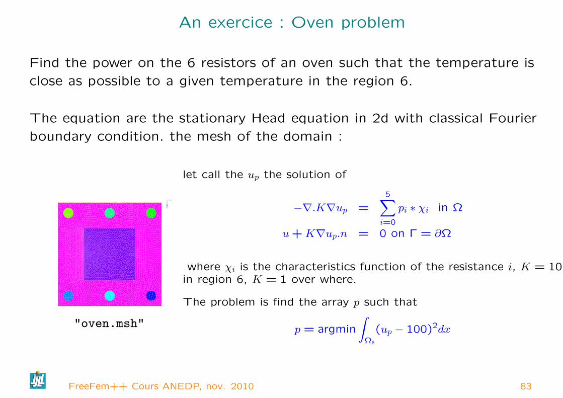
An exercice : Oven problem
Find the power on the 6 resistors of an oven such that the temperature is
close as possible to a given temperature in the region 6.
The equation are the stationary Head equation in 2d with classical Fourier
boundary condition. the mesh of the domain :
IsoValue012345678
"oven.msh"
let call the up the solution of
−∇.K∇up =5∑i=0
pi ∗ χi in Ω
u+K∇up.n = 0 on Γ = ∂Ω
where χi is the characteristics function of the resistance i, K = 10in region 6, K = 1 over where.
The problem is find the array p such that
p = argmin
∫Ω6
(up − 100)2dx
FreeFem++ Cours ANEDP, nov. 2010 83

Some remark
Xh[int] ur(6); // to store the 6 finite element functions Xh
To day, FreeFem++ have only linear solver on sparse matrix. so a way to solve
a full matrix problem is for example :
real[int,int] AP(6,6); // a full matrix
real[int] B(6),PR(6); // to array (vector of size 6)
... bla bla to compute AP and B
matrix A=AP; // build sparse data structure to store the full matrix
set(A,solver=CG); // set linear solver to the Conjuguate Gradient
PR=A^-1*B; // solve the linear system.
The file name of the mesh is oven.msh, and the region numbers are 0 to 5 for
the resitor, 6 for Ω6 and 7 for the rest of Ω and the label of Γ is 1.
FreeFem++ Cours ANEDP, nov. 2010 84
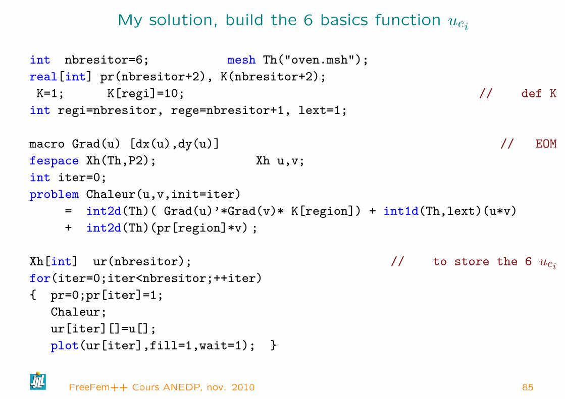
My solution, build the 6 basics function uei
int nbresitor=6; mesh Th("oven.msh");
real[int] pr(nbresitor+2), K(nbresitor+2);
K=1; K[regi]=10; // def K
int regi=nbresitor, rege=nbresitor+1, lext=1;
macro Grad(u) [dx(u),dy(u)] // EOM
fespace Xh(Th,P2); Xh u,v;
int iter=0;
problem Chaleur(u,v,init=iter)
= int2d(Th)( Grad(u)’*Grad(v)* K[region]) + int1d(Th,lext)(u*v)
+ int2d(Th)(pr[region]*v) ;
Xh[int] ur(nbresitor); // to store the 6 ueifor(iter=0;iter<nbresitor;++iter)
pr=0;pr[iter]=1;
Chaleur;
ur[iter][]=u[];
plot(ur[iter],fill=1,wait=1);
FreeFem++ Cours ANEDP, nov. 2010 85
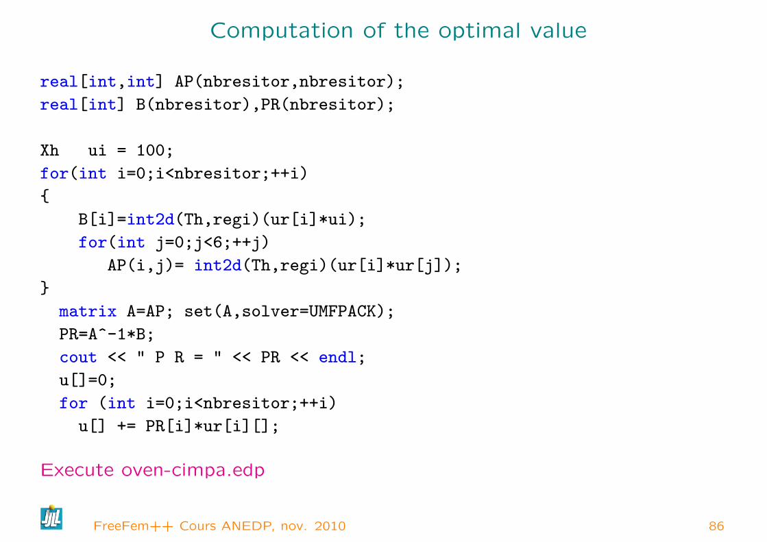
Computation of the optimal value
real[int,int] AP(nbresitor,nbresitor);
real[int] B(nbresitor),PR(nbresitor);
Xh ui = 100;
for(int i=0;i<nbresitor;++i)
B[i]=int2d(Th,regi)(ur[i]*ui);
for(int j=0;j<6;++j)
AP(i,j)= int2d(Th,regi)(ur[i]*ur[j]);
matrix A=AP; set(A,solver=UMFPACK);
PR=A^-1*B;
cout << " P R = " << PR << endl;
u[]=0;
for (int i=0;i<nbresitor;++i)
u[] += PR[i]*ur[i][];
Execute oven-cimpa.edp
FreeFem++ Cours ANEDP, nov. 2010 86

Stokes equation
The Stokes equation is find a velocity field u = (u1, .., ud) and the pressure pon domain Ω of Rd, such that
−∆u +∇p = 0 in Ω∇ · u = 0 in Ω
u = uΓ on Γ
where uΓ is a given velocity on boundary Γ.
The classical variationnal formulation is : Find u ∈ H1(Ω)d with u|Γ = uΓ,and p ∈ L2(Ω)/R = q ∈ L2(Ω)/
∫q = 0 such that
∀v ∈ H10(Ω)d, ∀q ∈ L2(Ω)/R,
∫Ω∇u : ∇v − p∇.v − q∇.u = 0
or now find p ∈ L2(Ω) such than (with ε = 10−10) ( Stabilize problem)
∀v ∈ H10(Ω)d, ∀q ∈ L2(Ω),
∫Ω∇u : ∇v − p∇.v − q∇.u+ εpq = 0
FreeFem++ Cours ANEDP, nov. 2010 87
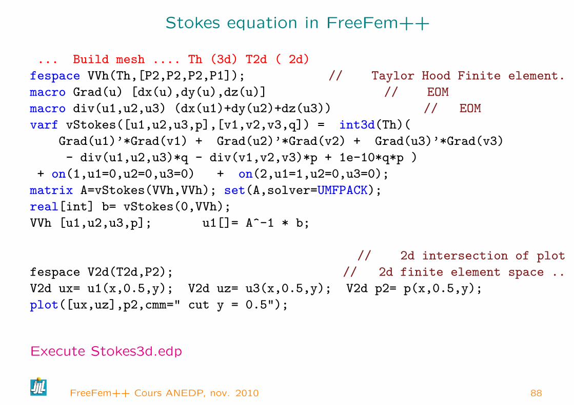
Stokes equation in FreeFem++
... Build mesh .... Th (3d) T2d ( 2d)
fespace VVh(Th,[P2,P2,P2,P1]); // Taylor Hood Finite element.
macro Grad(u) [dx(u),dy(u),dz(u)] // EOM
macro div(u1,u2,u3) (dx(u1)+dy(u2)+dz(u3)) // EOM
varf vStokes([u1,u2,u3,p],[v1,v2,v3,q]) = int3d(Th)(
Grad(u1)’*Grad(v1) + Grad(u2)’*Grad(v2) + Grad(u3)’*Grad(v3)
- div(u1,u2,u3)*q - div(v1,v2,v3)*p + 1e-10*q*p )
+ on(1,u1=0,u2=0,u3=0) + on(2,u1=1,u2=0,u3=0);
matrix A=vStokes(VVh,VVh); set(A,solver=UMFPACK);
real[int] b= vStokes(0,VVh);
VVh [u1,u2,u3,p]; u1[]= A^-1 * b;
// 2d intersection of plot
fespace V2d(T2d,P2); // 2d finite element space ..
V2d ux= u1(x,0.5,y); V2d uz= u3(x,0.5,y); V2d p2= p(x,0.5,y);
plot([ux,uz],p2,cmm=" cut y = 0.5");
Execute Stokes3d.edp
FreeFem++ Cours ANEDP, nov. 2010 88

incompressible Navier-Stokes equation with characteristicsmethods
∂u
∂t+ u · ∇u− ν∆u+∇p = 0, ∇ · u = 0
with the same boundary conditions and with initial conditions u = 0.
This is implemented by using the interpolation operator for the term∂u∂t + u · ∇u, giving a discretization in time
1τ (un+1 − un Xn)− ν∆un+1 +∇pn+1 = 0,
∇ · un+1 = 0(5)
The term Xn(x) ≈ x− un(x)τ will be computed by the interpolation
operator, or with convect operator (work form version 3.3)
FreeFem++ Cours ANEDP, nov. 2010 89
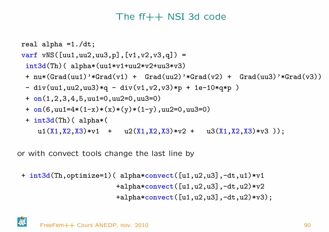
The ff++ NSI 3d code
real alpha =1./dt;
varf vNS([uu1,uu2,uu3,p],[v1,v2,v3,q]) =
int3d(Th)( alpha*(uu1*v1+uu2*v2+uu3*v3)
+ nu*(Grad(uu1)’*Grad(v1) + Grad(uu2)’*Grad(v2) + Grad(uu3)’*Grad(v3))
- div(uu1,uu2,uu3)*q - div(v1,v2,v3)*p + 1e-10*q*p )
+ on(1,2,3,4,5,uu1=0,uu2=0,uu3=0)
+ on(6,uu1=4*(1-x)*(x)*(y)*(1-y),uu2=0,uu3=0)
+ int3d(Th)( alpha*(
u1(X1,X2,X3)*v1 + u2(X1,X2,X3)*v2 + u3(X1,X2,X3)*v3 ));
or with convect tools change the last line by
+ int3d(Th,optimize=1)( alpha*convect([u1,u2,u3],-dt,u1)*v1
+alpha*convect([u1,u2,u3],-dt,u2)*v2
+alpha*convect([u1,u2,u3],-dt,u2)*v3);
FreeFem++ Cours ANEDP, nov. 2010 90

The ff++ NSI 3d code/ the loop in times
A = vNS(VVh,VVh); set(A,solver=UMFPACK); // build and factorize matrix
real t=0;
for(int i=0;i<50;++i)
t += dt; X1[]=XYZ[]-u1[]*dt; // set χ=[X1,X2,X3] vector
b=vNS(0,VVh); // build NS rhs
u1[]= A^-1 * b; // solve the linear systeme
ux= u1(x,0.5,y); uz= u3(x,0.5,y); p2= p(x,0.5,y);
plot([ux,uz],p2,cmm=" cut y = 0.5, time ="+t,wait=0);
Execute NSI3d.edp
FreeFem++ Cours ANEDP, nov. 2010 91

Newton Ralphson algorithm
Now, we solve the problem with Newton Ralphson algorithm, to solve the
problem F (u) = 0 the algorithm is
un+1 = un −(DF (un)
)−1F (un)
So we can rewrite :
un+1 = un − wn; DF (un)wn = F (un)
FreeFem++ Cours ANEDP, nov. 2010 92
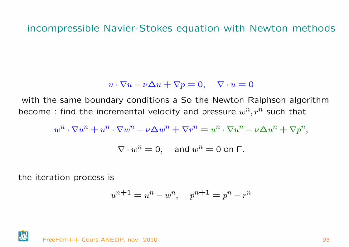
incompressible Navier-Stokes equation with Newton methods
u · ∇u− ν∆u+∇p = 0, ∇ · u = 0
with the same boundary conditions a So the Newton Ralphson algorithm
become : find the incremental velocity and pressure wn, rn such that
wn · ∇un + un · ∇wn − ν∆wn +∇rn = un · ∇un − ν∆un +∇pn,
∇ · wn = 0, and wn = 0 on Γ.
the iteration process is
un+1 = un − wn, pn+1 = pn − rn
FreeFem++ Cours ANEDP, nov. 2010 93

Solve incompressible Navier Stokes flow (3 Slides)
// define finite element space Taylor Hood.fespace XXMh(th,[P2,P2,P1]);XXMh [u1,u2,p], [v1,v2,q];
// macromacro div(u1,u2) (dx(u1)+dy(u2)) //macro grad(u1,u2) [dx(u1),dy(u2)] //macro ugrad(u1,u2,v) (u1*dx(v)+u2*dy(v)) //macro Ugrad(u1,u2,v1,v2) [ugrad(u1,u2,v1),ugrad(u1,u2,v2)] //
// solve the Stokes equationsolve Stokes ([u1,u2,p],[v1,v2,q],solver=UMFPACK) =
int2d(th)( ( dx(u1)*dx(v1) + dy(u1)*dy(v1)+ dx(u2)*dx(v2) + dy(u2)*dy(v2) )+ p*q*(0.000001)- p*div(v1,v2) - q*div(u1,u2) )
+ on(1,u1=u1infty,u2=u2infty)+ on(3,u1=0,u2=0);
real nu=1./100.;
FreeFem++ Cours ANEDP, nov. 2010 94
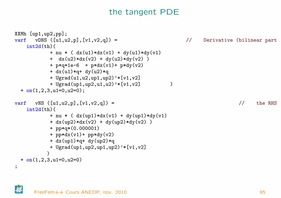
the tangent PDE
XXMh [up1,up2,pp];varf vDNS ([u1,u2,p],[v1,v2,q]) = // Derivative (bilinear part
int2d(th)(+ nu * ( dx(u1)*dx(v1) + dy(u1)*dy(v1)+ dx(u2)*dx(v2) + dy(u2)*dy(v2) )+ p*q*1e-6 + p*dx(v1)+ p*dy(v2)+ dx(u1)*q+ dy(u2)*q+ Ugrad(u1,u2,up1,up2)’*[v1,v2]+ Ugrad(up1,up2,u1,u2)’*[v1,v2] )
+ on(1,2,3,u1=0,u2=0);
varf vNS ([u1,u2,p],[v1,v2,q]) = // the RHSint2d(th)(
+ nu * ( dx(up1)*dx(v1) + dy(up1)*dy(v1)+ dx(up2)*dx(v2) + dy(up2)*dy(v2) )+ pp*q*(0.000001)+ pp*dx(v1)+ pp*dy(v2)+ dx(up1)*q+ dy(up2)*q+ Ugrad(up1,up2,up1,up2)’*[v1,v2])
+ on(1,2,3,u1=0,u2=0);
FreeFem++ Cours ANEDP, nov. 2010 95
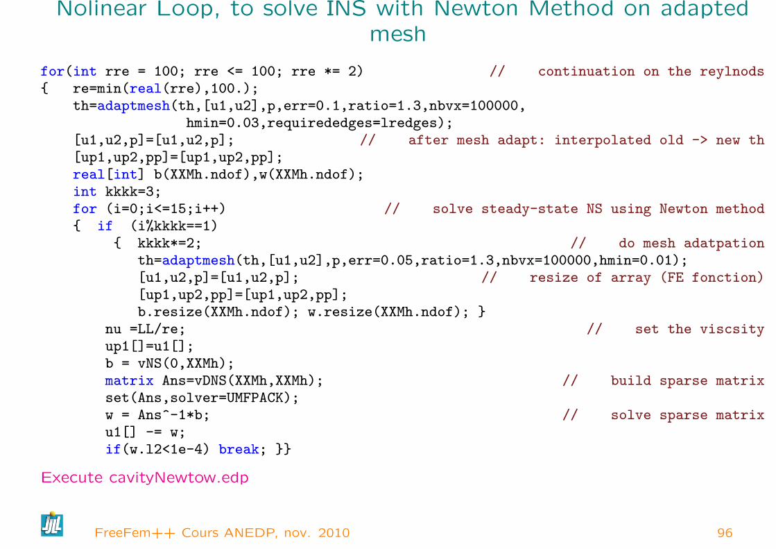
Nolinear Loop, to solve INS with Newton Method on adaptedmesh
for(int rre = 100; rre <= 100; rre *= 2) // continuation on the reylnods re=min(real(rre),100.);
th=adaptmesh(th,[u1,u2],p,err=0.1,ratio=1.3,nbvx=100000,hmin=0.03,requirededges=lredges);
[u1,u2,p]=[u1,u2,p]; // after mesh adapt: interpolated old -> new th[up1,up2,pp]=[up1,up2,pp];real[int] b(XXMh.ndof),w(XXMh.ndof);int kkkk=3;for (i=0;i<=15;i++) // solve steady-state NS using Newton method if (i%kkkk==1)
kkkk*=2; // do mesh adatpationth=adaptmesh(th,[u1,u2],p,err=0.05,ratio=1.3,nbvx=100000,hmin=0.01);[u1,u2,p]=[u1,u2,p]; // resize of array (FE fonction)[up1,up2,pp]=[up1,up2,pp];b.resize(XXMh.ndof); w.resize(XXMh.ndof);
nu =LL/re; // set the viscsityup1[]=u1[];b = vNS(0,XXMh);matrix Ans=vDNS(XXMh,XXMh); // build sparse matrixset(Ans,solver=UMFPACK);w = Ans^-1*b; // solve sparse matrixu1[] -= w;if(w.l2<1e-4) break;
Execute cavityNewtow.edp
FreeFem++ Cours ANEDP, nov. 2010 96
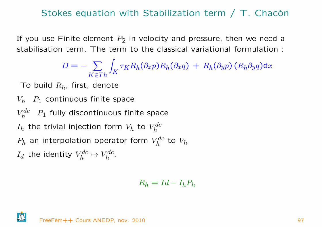
Stokes equation with Stabilization term / T. Chacon
If you use Finite element P2 in velocity and pressure, then we need a
stabilisation term. The term to the classical variational formulation :
D = −∑
K∈Th
∫KτKRh(∂xp)Rh(∂xq) + Rh(∂yp) (Rh∂yq)dx
To build Rh, first, denote
Vh P1 continuous finite space
V dch P1 fully discontinuous finite space
Ih the trivial injection form Vh to V dch
Ph an interpolation operator form V dch to Vh
Id the identity V dch 7→ V dch .
Rh = Id− IhPh
FreeFem++ Cours ANEDP, nov. 2010 97
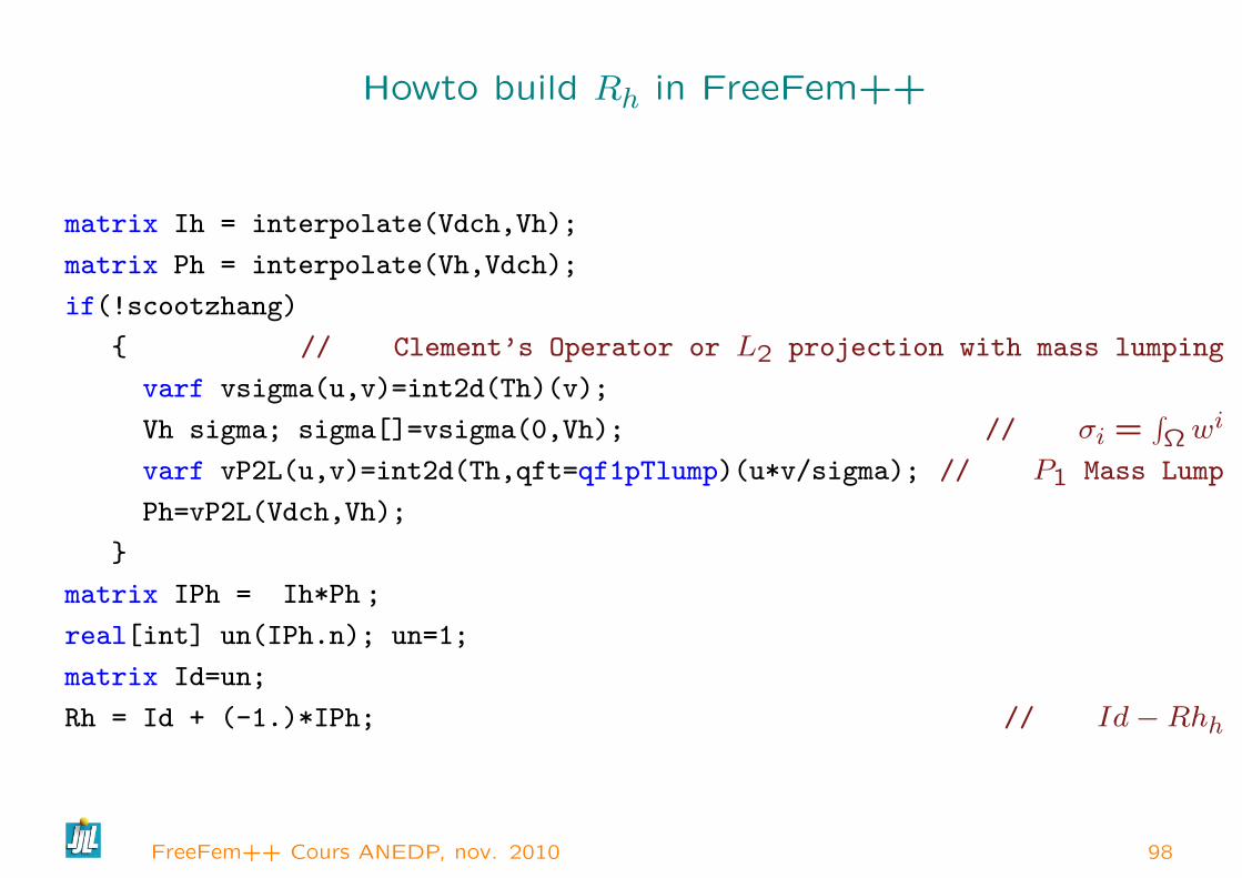
Howto build Rh in FreeFem++
matrix Ih = interpolate(Vdch,Vh);
matrix Ph = interpolate(Vh,Vdch);
if(!scootzhang)
// Clement’s Operator or L2 projection with mass lumping
varf vsigma(u,v)=int2d(Th)(v);
Vh sigma; sigma[]=vsigma(0,Vh); // σi =∫Ωwi
varf vP2L(u,v)=int2d(Th,qft=qf1pTlump)(u*v/sigma); // P1 Mass Lump
Ph=vP2L(Vdch,Vh);
matrix IPh = Ih*Ph ;
real[int] un(IPh.n); un=1;
matrix Id=un;
Rh = Id + (-1.)*IPh; // Id−Rhh
FreeFem++ Cours ANEDP, nov. 2010 98

Howto build the D matrix in FreeFem++
....fespace Wh(Th,[P2,P2,P2]); // the Stokes FE Spacefespace Vh(Th,P1); fespace Vdch(Th,P1dc);....matrix D; // the variable to store the matrix D varf vMtk(p,q)=int2d(Th)(hTriangle*hTriangle*ctk*p*q);matrix Mtk=vMtk(Vdch,Vdch);int[int] c2=[2]; // take the 2 second component of Wh.matrix Dx = interpolate(Vdch,Wh,U2Vc=c2,op=1); // ∂xp discrete operatormatrix Dy = interpolate(Vdch,Wh,U2Vc=c2,op=2); // ∂yp discrete operatormatrix Rh;
... add Build of Rh code hereDx = Rh*Dx; Dy = Rh*Dy;
// Sorry matrix operation is done one by one.matrix DDxx= Mtk*Dx; DDxx = Dx’*DDxx;matrix DDyy= Mtk*Dy; DDyy = Dy’*DDyy;D = DDxx + DDyy;
// cleaning all local matrix and array.A = A + D; // add to the Stokes matrix....
Execute Stokes-tomas.edp
FreeFem++ Cours ANEDP, nov. 2010 99

Conclusion and Future
It is a useful tool to teaches Finite Element Method, and to test some
nontrivial algorithm.
– Optimization FreeFem++ in 3d
– All graphic with OpenGL (in construction)
– Galerkin discontinue (fait in 2d, a faire in 3d)
– complex problem (fait)
– 3D ( under construction )
– automatic differentiation ( under construction )
– // linear solver and build matrix //
– 3d mesh adaptation
– Suite et FIN. (L’avenir ne manque pas de future et lycee de Versailles)
Thank, for your attention ?
FreeFem++ Cours ANEDP, nov. 2010 100