FreeFem++, part I

M. M. Sussmansussmanm@math.pitt.edu

Office Hours: 11:10AM-12:10PM, Thack 622

May 12 – June 19, 2014

1 / 76

Incompressible NSE

∂u∂t

+ u · ∇u − ν∆u +∇p = f

∇ · u = 0

L R1L1 R1

B

T

B1

T1

4 / 76

example18.edp Vortex shedding past a square

example18.edp

5 / 76

example18.edp Code outline

1. Generate/plot geometry2. Generate/plot mesh3. Specify finite element spaces and instantiate variables4. Construct weak form with b.c.5. Time loop

5.1 Update time-dependent b.c.5.2 Solve5.3 Plot

6 / 76

Some syntax (C++)

I Comments preceeded by //I Can also use /* ... */I Good for multiline comments

I Commands mostly end with semicolonI No need for a line continuation character

I Extra spaces and indentation don’t matterI Variables must have a specified typeI “Curly brackets” () used for groupingI Single quotes for characters (’a’)I Double quotes for strings ("Hello there")

7 / 76

example18.edp Geometry

L R1L1 R1

B

T

B1

T1

real L=0.0, R=2.0, B=0.0, T=1.0;real L1=0.2, R1=0.4, B1=0.4, T1=0.6;int nx=20, ny=10, nx1=5, ny1=5;

// outer squareborder Bottom( t=0,1 )x= L + (R-L)*t; y= B; label= 1;;

// obstacleborder ObsBottom( t=0,1 )x= L1 + (R1-L1)*t; y= B1; label= 5;;

plot( Bottom(nx) + Right(ny) + Top(-nx) + Left(-ny)+ ObsBottom(-nx1) + ObsRight(-ny1) + ObsTop(+nx1)+ ObsLeft(+ny1), wait=1 );

9 / 76

example18.edp Code// Example 18: Vortex shedding past a square

real L= 0.0, R= 2.0, B= 0.0, T= 1.0;real L1= 0.2, R1= 0.4, B1= 0.4, T1= 0.6;int nx=20, ny=10;int nx1=5, ny1=5;

// outer squareborder Bottom( t=0,1 )x= L + (R-L)*t; y= B; label= 1;;border Top( t=0,1 )x= L + (R-L)*t; y= T; label= 3;;border Left( t=0,1 )x= L; y= B + (T-B)*t; label= 4;;border Right( t=0,1 )x= R; y= B + (T-B)*t; label= 2;;

// obstacleborder ObsBottom(t= 0,1)x= L1 + (R1-L1)*t; y= B1; label= 5;;border ObsTop(t= 0,1)x= L1 + (R1-L1)*t; y= T1; label= 7;;border ObsLeft(t= 0,1)x= L1; y= B1 + (T1-B1)*t; label= 8;;border ObsRight(t= 0,1)x= R1; y= B1 + (T1-B1)*t; label= 6;;

// plot geometryplot( Bottom(nx) + Right(ny) + Top(-nx) + Left(-ny)

+ ObsBottom(-nx1) + ObsRight(-ny1) + ObsTop(+nx1) + ObsLeft(+ny1), wait=1 );

// generate meshmesh Th= buildmesh( Bottom(nx) + Right(ny) + Top(-nx) + Left(-ny)

+ ObsBottom(-nx) + ObsRight(-ny) + ObsTop(+nx) + ObsLeft(+ny) );

// plot meshplot(Th, wait=1, ps="VortexStreetMesh.eps");

10 / 76

Geometry plot

11 / 76

Mesh plot

12 / 76

example18.edp Code, cont’d

fespace Xh( Th, P2);fespace Mh( Th, P1);Xh u2, v2, u1, v1, up1, up2;Mh p, q;

int numTSteps=600;bool reuseMatrix = false;real nu=1./1000., dt=0.05, bndryVelocity;

problem NS ([u1, u2, p] , [v1, v2, q] , init= reuseMatrix) =int2d(Th)( 1./dt * ( u1*v1 + u2*v2 )

+ nu * ( dx(u1)*dx(v1) + dy(u1)*dy(v1)+ dx(u2)*dx(v2) + dy(u2)*dy(v2) )+ p*q*(0.000001)+ p*dx(v1) + p*dy(v2)+ dx(u1)*q + dy(u2)*q ) MORE ...

+ int2d(Th) ( -1./dt*convect( [up1, up2] , -dt , up1) * v1-1./dt*convect( [up1, up2] , -dt , up2) * v2 )

MORE ...// b.c.: uniform velocity top, bottom, inlet (left)// "do nothing" on exit (right)

+ on(1, u1=bndryVelocity, u2=0)+ on(3, u1=bndryVelocity, u2=0)+ on(4, u1=bndryVelocity, u2=0)+ on(5, 6, 7, 8, u1=0, u2=0);

14 / 76

New keywords and functions

real(int)bordermeshbuildmeshfespaceproblemint2ddx, dy( ... )on (for boundary conditions)convect

15 / 76

What is convect?

I Section 9.5.2 of the FreeFem++ book, p. 240ff.I Note that

∂w∂t

+ u · ∇w =dw(X (t), t)

dtwhere

dX (t)dt

= u(X (t), t)

I Given a point x , find the solution of the “final value problem”dX/dt = um(X (t)), with X (tm+1) = x ,

I Then

dw(X (t), t)dt

≈ w(X (tm+1), tm+1)− w(X (tm), tm)

∆t

=wm+1 − w(X (tm), tm)

∆t

I How to get w(X (tm), tm)?

17 / 76

The “final value problem” for convect?

I Assume wm(x) is a known function of xI Assume u(x , t) ≈ um(x) is constant over the interval

tm ≤ t < tm+1

I X (tm+1)− X (tm) ≈ ∆tum(X (tm+1))

I Solving, x(tm) = x − um(x)∆tI w(X (tm), tm) = w(x − um∆t)I convect(u,-dt,w)(x) = w(x − u dt)

18 / 76

That sounds great! Why doesn’t everyone do it?

I Those approximations are O(∆t)I What if the flow is fast enough so x − u dt is out of the element?I What if the flow is fast enough so x − u dt is out of Ω?I Hard to prove things about.I Stability?

19 / 76

More syntax

I Declare a real vector: real[int] v(100);I Loopingfor (int index=0 ; index < maximum ; i++) ... code ...

I Can use an already-declared index variable.I index is no longer “in scope” after the loop ends

21 / 76

Scoping, blocking and variable declarations

I Variables can be declared anywhere in the programI “Blocks” of code are inside curly brackets: ... I Declarations inside a block:

I Are not known outside the block.I “Cover up” previous declarations

22 / 76

Asking questions: if

boolean expression ? true expression : false expression

if ( boolean expression )... code ...

if ( boolean expression )... code ...

else if ... code ...

else ... code ...

A single statement does not need to be inside a block.

23 / 76

Boolean expressions

Comparison operatorsoperator description== equal to!= not equal to< less than<= less than or equal to>= greater than or equal to

Logical operatorsoperator description! not&& and|| or

Do not use & or |! They are bitwise operators.

Remark: Logical operators are “short circuit”

24 / 76

example18.edp Code, cont’d

real[int] times(numTSteps), var(numTSteps);

for (int i=0 ; i < numTSteps ; i++)times[i] = i*dt;

// ramp up velocity from 0.0bndryVelocity = i*dt;if (bndryVelocity >= 1.0)

bndryVelocity = 1.0;

up1 = u1;up2 = u2;

// Solve the problemNS;

// reuse the matrix in the rest of the iterationsreuseMatrix = true

// plot current solutionplot(coef=0.2, cmm= " [u1,u2] and p ", p, [u1,u2]

ArrowShape= 1, ArrowSize= -0.8);

25 / 76

Exercise 22 (10 points)

Example 18 presents a vortex-shedding problem using the“convect” function in FreeFem++. Convert the code to use theconventional form of the convection terms. You should observe vortexshedding behavior in your formulation, although details may differ.Explain any differences you think are important between the twosolutions.

26 / 76

Comparison with FEniCS code: boundary conditions

I FreeFem++ code goes into the weak form+ on(1, u1=bndryVelocity, u2=0)+ on(3, u1=bndryVelocity, u2=0)+ on(4, u1=bndryVelocity, u2=0)+ on(5, 6, 7, 8, u1=0, u2=0)

I FEniCS code requires a mesh functionboundaries = MeshFunction("size_t", mesh, mesh.topology().dim()-1)

I FEniCS code requires new classesclass InflowBoundary(SubDomain):

def inside(self, x, on_boundary):return on_boundary and x[0] < xmin + bmarg

I FEniCS requires instantiationinflowBoundary = InflowBoundary()g1 = Expression( ("4.*Um*(x[1]*(ymax-x[1]))/(ymax*ymax)" , "0.0"), \

Um=1.5, ymax=ymax)bc1 = DirichletBC(W.sub(0), g1, inflowBoundary)

I FEniCS then has the b.c.s passed to the solver with the matrices.solve(NSE == LNSE, w, bcs)

27 / 76

Comparison with FEniCS code: functions and spaces

I FEniCS:V = VectorFunctionSpace(mesh, "CG", 2)Q = FunctionSpace(mesh, "CG", 1)W = V * Q

...(u, p) = TrialFunctions(W)(v, q) = TestFunctions(W)w = Function(W)u0 = Function(V)

I FreeFem++fespace Xh( Th, P2);fespace Mh( Th, P1);Xh u2, v2, u1, v1, up1, up2;Mh p, q;

28 / 76

Comparison with FEniCS code: Weak form

I FEniCSLNSE = inner(u0,v)*dxNSE = (inner(u,v) + dt*(inner(grad(u)*u0,v) \

+ nu*inner(grad(u),grad(v)) - div(v)*p) + q*div(u) )*dx

I FreeFem++problem NS ([u1, u2, p] , [v1, v2, q] =

int2d(Th)( 1./dt*( u1*v1 + u2*v2 )+ nu * ( dx(u1)*dx(v1) + dy(u1)*dy(v1)+ dx(u2)*dx(v2) + dy(u2)*dy(v2) )+ p*q*(0.000001)+ p*dx(v1) + p*dy(v2)+ dx(u1)*q + dy(u2)*q )

+ int2d(Th) ( -1./dt*convect( [up1, up2] , -dt , up1) * v1-1./dt*convect( [up1, up2] , -dt , up2) * v2 )

plus b.c.s

29 / 76

I’d like to print some stuff.

I Printing uses cout and <<I Add lines inside the loop

cout << "t=" << times[i] << " umax="<< max(u1[].max, u2[].max)<< " vertical velocity=" << u2(0.5, 0.5) << endl;

30 / 76

Can I put some stuff into a file?I Place file definition and use inside a blockI File is closed when it goes out of scope

ofstream vels("vels.txt");for (i=0 ; i < numTSteps ; i++)

// ramp up velocity from 0.0bndryVelocity = i*dt;if (bndryVelocity >= 1.0)

bndryVelocity = 1.0;

up1 = u1;up2 = u2;

// solve the problemNS;

// reuse the matrix in the rest of the iterationsreuseMatrix = true;

// write a 2-column file (t,velocity)vels << i*dt << " " << u2(0.5, 0.5) << endl;

// file is closed

31 / 76

example19.edp Poisson’s equation on a circle

−∆u(x , y) = f (x , y) inside Ω

u(x , y) = 0 on ∂Ω

where Ω is the unit circle in R2.

33 / 76

example19.edp code

// defining the boundaryborder C(t=0,2*pi)x=cos(t); y=sin(t);// the triangulated domain Th is on the left side of its boundary// because boundary parameterization is CCW

// mesh based on 50 t-incrementsmesh Th = buildmesh (C(50));

Remark: Mesh boundary is polygonal, not curved. P2 elements willhave extra boundary nodes off the circle.

34 / 76

example19.edp code

// the finite element space defined over Th is called here Vhfespace Vh(Th,P1);

Vh u,v; // defines u and v as piecewise-P1 continuous functions

func f= x*y; // definition of a function named f for RHS

real cpu = clock(); // get the clock in second

solve Poisson(u, v, solver=UMFPACK) = // defines the PDEint2d(Th)( dx(u)*dx(v) + dy(u)*dy(v) ) // bilinear part- int2d(Th)( f*v ) // right hand side+ on(C, u=0) ; // Dirichlet boundary condition

plot(u, ps="solution19.eps"); // plot solution

cout << " CPU time = " << clock()-cpu << endl; // print time required

35 / 76

Some more syntax

I Book Chapter 4I Variables: real, int, bool, complexI Variable names: letters and numbers, no _I File variables: ofstream, ifstreamI Global variables: cout, cin, true, false, pi, iI Arrays: real[int]

37 / 76

Global variables (used mainly in weak forms)

I For current pointI x, y, zI label (boundary point label, 0 if not boundary)I regionI P, P.x, P.y, P.zI N, N.x, N.y, N.z

I lenEdge length of current edgeI hTriangle size of current triangleI area area of current triangleI volume volume of current triangleI nuTriangle number (int) of current triangleI nuEdge number (int) of current edgeI nuTonEdge number (int) of adjacent triangle

38 / 76

Operations and functions

I Usual arithmetic operatorsI Raise to power ˆI Usual elementary functions (sin, acosh, etc.)I randres53 generates uniform reals in [0,1) with 53-bit

resolution

39 / 76

Functions

I func declares a functionI Simple example

func u = x2 + sin(pi*y)

I With declarationsfunc real u( int k)return 3.0*k*k;

I With arraysfunc real[int] sqarr( int[int] L, int n)real[int] ans(n);for (int k=0; k<n ; k++)ans[k]=L[k]^2;

return ans;

I Examples→ tutorial/func.edp

40 / 76

Exercise 23 (5 points)

The following example is presented in Chapter 4.

mesh Th=square(20,20,[-pi+2*pi*x,-pi+2*pi*y]); // [-pi,pi] X [-pi,pi]fespace Vh(Th,P2);func z=x+y*1i; // x+iyfunc f=imag(sqrt(z));func g=abs( sin(z/10)*exp(z^2/10) ); // complex argumentsVh fh = f;plot(fh); // contours of fVh gh = g;plot(gh); // contours of g

I Copy this to a file, run FreeFem++, and send me the plots.I Change the mesh so that the base of the square is oriented at an

angle of π/4 instead of being horizontal. Send me the changedcode and the resulting plots.

41 / 76

Array operations

int i;real [int] tab(10), tab1(10); // 2 array of 10 realcomplex [int] ctab(10), ctab1(10); // 2 array of 10 complex

tab = 1; // set all the array to 1tab[1] = 2;ctab = 1+2i; // set all the array to 1+2ictab[1] = 2;cout << "tab: " << tab[1] << " " << tab[9] << " size = " << tab.n << endl;cout << "ctab: " << ctab[1] << " " << ctab[9] << " size = " << ctab.n << endl;

Yields as output

tab: 2 1 size = 10ctab: (2,0) (1,2) size = 10

42 / 76

Array operations, cont’d

tab1 = tab;tab = tab + tab1;tab = 2*tab + tab1*5;tab1 = 2*tab - tab1*5;tab += tab;cout << "whole array tab = " << tab << endl;cout << "tab[1] = " << tab[1] << " tab[9] = " << tab[9] << endl;

Yields as output

whole array tab = 1018 36 18 18 1818 18 18 18 18

tab[1] = 36 tab[9] = 18

43 / 76

Array operations, cont’d

ctab1 = ctab;ctab = ctab + ctab1;ctab = 2*ctab + ctab1*5;ctab1 = 2*ctab - ctab1*5;ctab += ctab;cout << "whole array ctab = " << ctab << endl;cout << "ctab[1] = " << ctab[1] << " ctab[9] = " << ctab[9] << endl << endl;

Yields as output

whole array ctab = 10(18,36) (36,0) (18,36) (18,36) (18,36)(18,36) (18,36) (18,36) (18,36) (18,36)

ctab[1] = (36,0) ctab[9] = (18,36)

44 / 76

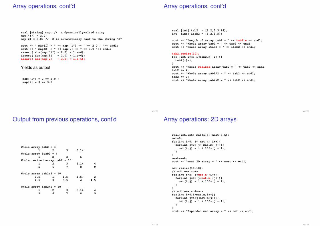
Array operations, cont’d

real [string] map; // a dynamically-sized arraymap["1"] = 2.0;map[2] = 3.0; // 2 is automaticaly cast to the string "2"

cout << " map[1] = " << map["1"] << " == 2.0 ; "<< endl;cout << " map[2] = " << map[2] << " == 3.0 "<< endl;assert( abs(map["1"] - 2.0) < 1.e-6);assert( abs(map[1] - 2.0) < 1.e-6);assert( abs(map[2] - 3.0) < 1.e-6);

Yields as output

map["1"] = 2 == 2.0 ;map[2] = 3 == 3.0

45 / 76

Array operations, cont’d

real [int] tab2 = [1,2,3,3.14];int [int] itab2 = [1,2,3,5];

cout << "Length of array tab2 = " << tab2.n << endl;cout << "Whole array tab2 = " << tab2 << endl;cout << "Whole array itab2 = " << itab2 << endl;

tab2.resize(10);for (int i=4; i<tab2.n; i++)

tab2[i]=i;cout << "Whole resized array tab2 = " << tab2 << endl;tab2 /= 2;cout << "Whole array tab2/2 = " << tab2 << endl;tab2 *= 2;cout << "Whole array tab2*2 = " << tab2 << endl;

46 / 76

Output from previous operations, cont’d

Whole array tab2 = 41 2 3 3.14

Whole array itab2 = 41 2 3 5

Whole resized array tab2 = 101 2 3 3.14 45 6 7 8 9

Whole array tab2/2 = 100.5 1 1.5 1.57 22.5 3 3.5 4 4.5

Whole array tab2*2 = 101 2 3 3.14 45 6 7 8 9

47 / 76

Array operations: 2D arrays

real[int,int] mat(5,5),mmat(5,5);mat=0;for(int i=0; i< mat.n; i++)

for(int j=0; j< mat.m; j++)mat(i,j) = i + 100*(j + 1);

mmat=mat;cout << "mmat 2D array = " << mmat << endl;

mat.resize(10,10);// add new rowsfor(int i=5; i<mat.n ;i++)

for(int j=0; j<mat.m ;j++)mat(i,j) = i + 100*(j + 1);

// add new columnsfor(int i=0;i<mat.n;i++)

for(int j=5;j<mat.m;j++)mat(i,j) = i + 100*(j + 1);

cout << "Expanded mat array = " << mat << endl;

48 / 76

Output from previous operations, cont’d

mmat 2D array = 5 5100 200 300 400 500101 201 301 401 501102 202 302 402 502103 203 303 403 503104 204 304 404 504

Expanded mat array = 10 10100 200 300 400 500 600 700 800 900 1000101 201 301 401 501 601 701 801 901 1001102 202 302 402 502 602 702 802 902 1002103 203 303 403 503 603 703 803 903 1003104 204 304 404 504 604 704 804 904 1004105 205 305 405 505 605 705 805 905 1005106 206 306 406 506 606 706 806 906 1006107 207 307 407 507 607 707 807 907 1007108 208 308 408 508 608 708 808 908 1008109 209 309 409 509 609 709 809 909 1009

49 / 76

Array operations: 1D array of mesh

mesh[int] aTh(10);aTh[1]= square(2,2);plot(aTh[1]);aTh[2]= square(3,4);plot(aTh[2]);

50 / 76

Example 20: Section 3.1

−∆φ = f in Ω

I Elastic membrane Ω

I Rigid support Γ, may have vertical displacementI Γ is ellipseI Load fI Solving for vertical displacement, φI Membrane glued to Γ: Dirichlet b.c.I Membrane free at Γ: Neumann b.c.I New:

I Both Dirichlet and Neumann b.c.I Accessing values from mesh and solutionI Write a plot file for gnuplot

54 / 76

example20.edp code

// example20.edp// original file: membrane.edp

real theta = 4.*pi/3.;real a = 2.,b = 1.; // semimajor and semiminor axes

func bndryelev = x; // elevation of Gamma1 boundary

border Gamma1(t=0, theta) x = a * cos(t); y = b*sin(t); border Gamma2(t=theta, 2*pi) x = a * cos(t); y = b*sin(t); mesh Th = buildmesh( Gamma1(100) + Gamma2(50) ); // construct mesh

fespace Vh(Th,P2); // P2 conforming triangular FEMVh phi,w, f=1; // phi is shape function, w is test function, f is load

// problem definitionsolve Laplace(phi, w) = int2d(Th)( dx(phi)*dx(w) + dy(phi)*dy(w) )

- int2d(Th)( f*w ) + on(Gamma1, phi= bndryelev);

plot(phi, wait=true, ps="solution20.eps"); //Plot solution

plot(Th, wait=true, ps="mesh20.eps"); //Plot mesh

55 / 76

Plot solution

56 / 76

Plot mesh

57 / 76

gnuplot file

I Gnuplot file has groups of 4 lines, each with a vertex location andvalue xj , yj , φj for j = 0,1,2,0 followed by a blank line.

I Commands for gnuplot areset palette rgbformulae 30,31,32splot "graph.txt" with lines palette

58 / 76

example20.edp code cont’d

// to build a gnuplot data file ofstream ff("graph20.txt");

for (int i=0;i<Th.nt;i++)for (int j=0; j <3; j++)

ff << Th[i][j].x <<" "<< Th[i][j].y <<" "<< phi[][Vh(i,j)] << endl;ff << Th[i][0].x << " " << Th[i][0].y<< " " << phi[][Vh(i,0)]

<< endl << endl << endl;

Th.nt is number of triangles in Th.Th[i][j].x is x-coordinate of vertex j of triangle i in the meshphi[][Vh(i,j)] is the value of dof of φ located at vertex j oftriangle i in fespace Vh. The extra dofs have numbers 3 and higher.

59 / 76

Demonstration (for Example20)

$ gnuplot

gnuplot> set palette rgbformulae 30,31,32gnuplot> splot "graph.txt" with lines palette

60 / 76

Example 21: errors

I from membranerror.edpI Like Example 20I Change to have exact solutionI Look at errors and convergenceI New:

I Turning off extraneous outputI Plot Th and phi togetherI Loading extra elements

62 / 76

example21.edp codeverbosity=0;

load "Element_P3"

real theta = 4.*pi/3.;real a=1., b=1.; // ellipse is a circle hereborder Gamma1(t=0.0,theta) x = a * cos(t); y = b*sin(t); border Gamma2(t=theta,2.0*pi) x = a * cos(t); y = b*sin(t);

func f=-4.0*(cos(x^2+y^2-1.0) -(x^2+y^2)*sin(x^2+y^2-1.0));func phiexact=sin(x^2+y^2-1.0);

int meshes=3, mshdensity=1;real[int] L2error(meshes);for ( int n=0; n<meshes; n++)

mesh Th = buildmesh( Gamma1(40*mshdensity) + Gamma2(20*mshdensity) );mshdensity *= 2;fespace Vh(Th,P2);Vh phi,w;

solve laplace(phi, w, solver=UMFPACK) =int2d(Th)( dx(phi) * dx(w) + dy(phi) * dy(w))- int2d(Th)( f*w ) + on(Gamma2, phi=0)+ on(Gamma1, phi=0);

phi = (phi-phiexact);plot(Th, phi, wait=true, fill=true); //Plot Th and phi

// compute errorL2error[n]= sqrt( int2d(Th)( (phi)^2 ) );

63 / 76

example21.edp code cont’d

// print errorsfor (int n=0; n<meshes; n++)

cout << " L2error " << n << " = "<< L2error[n] <<endl;

// print convergence ratesfor (int n=1; n<meshes; n++)

cout <<" convergence rate = "<< log( L2error[n-1] / L2error[n] )/log(2.)<<endl;

64 / 76

Output

L2error 1 = 0.000816958L2error 2 = 0.000203404L2error 3 = 5.07361e-05convergence rate = 2.01175convergence rate = 2.00592convergence rate = 2.00326

Error rates too slow!

65 / 76

Error on coarsest mesh

Maximum errors are near boundary because of geometry errors.

66 / 76

Change boundary condition

Change fromon(Gamma2, phi=0)toon(Gamma2, phi=phiexact)

Output:

L2error 1 = 8.05871e-08L2error 2 = 5.4554e-09L2error 3 = 3.30556e-10convergence rate = 4.31729convergence rate = 3.88479convergence rate = 4.04472

67 / 76

WARNING: special elements need FreeFem++-cs

LD_LIBRARY_PATH needs proper definition

68 / 76

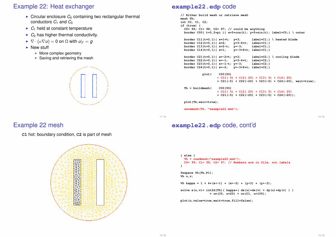
Example 22: Heat exchangerI Circular enclosure C0 containing two rectangular thermal

conductors C1 and C2

I C1 held at constant temperatureI C2 has higher thermal conductivity.I ∇ · (κ∇u) = 0 on Ω with u|Γ = gI New stuff

I More complex geometryI Saving and retrieving the mesh

71 / 76

example22.edp code// Either build mesh or retrieve meshmesh Th;int C0, C1, C2;if (true)

C0= 99; C1= 98; C2= 97; // could be anythingborder C00( t=0,2*pi ) x=5*cos(t); y=5*sin(t); label=C0; \ outer

border C11(t=0,1) x=1+t; y=3; label=C1; \ heated bladeborder C12(t=0,1) x=2; y=3-6*t; label=C1;border C13(t=0,1) x=2-t; y=-3; label=C1;border C14(t=0,1) x=1; y=-3+6*t; label=C1;

border C21(t=0,1) x=-2+t; y=3; label=C2; \ cooling bladeborder C22(t=0,1) x=-1; y=3-6*t; label=C2;border C23(t=0,1) x=-1-t; y=-3; label=C2;border C24(t=0,1) x=-2; y=-3+6*t; label=C2;

plot( C00(50)+ C11( 5) + C12( 20) + C13( 5) + C14( 20)+ C21(-5) + C22(-20) + C23(-5) + C24(-20), wait=true);

Th = buildmesh( C00(50)+ C11( 5) + C12( 20) + C13( 5) + C14( 20)+ C21(-5) + C22(-20) + C23(-5) + C24(-20));

plot(Th,wait=true);

savemesh(Th, "example22.msh");

72 / 76

Example 22 meshC1 hot: boundary condition, C2 is part of mesh

73 / 76

example22.edp code, cont’d

else Th = readmesh("example22.msh");C0= 99; C1= 98; C2= 97; // Numbers are in file, not labels

fespace Vh(Th,P1);Vh u,v;

Vh kappa = 1 + 4*(x<-1) * (x>-2) * (y<3) * (y>-3);

solve a(u,v)= int2d(Th)( kappa*( dx(u)*dx(v) + dy(u)*dy(v) ) )+ on(C0, u=20) + on(C1, u=100);

plot(u,value=true,wait=true,fill=false);

74 / 76

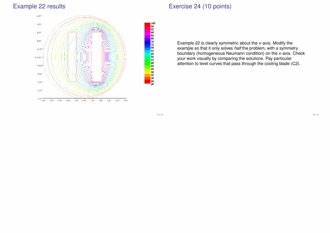
Example 22 results

75 / 76

Exercise 24 (10 points)

Example 22 is clearly symmetric about the x-axis. Modify theexample so that it only solves half the problem, with a symmetryboundary (homogeneous Neumann condition) on the x-axis. Checkyour work visually by comparing the solutions. Pay particularattention to level curves that pass through the cooling blade (C2).

76 / 76