FORWARD SELECTION OF EXPLANATORY VARIABLES

Ecology, 89(9), 2008, pp. 2623–2632� 2008 by the Ecological Society of America

FORWARD SELECTION OF EXPLANATORY VARIABLES

F. GUILLAUME BLANCHET,1 PIERRE LEGENDRE, AND DANIEL BORCARD

Departement de Sciences Biologiques, Universite de Montreal, C.P. 6128, Succursale Centre-ville, Montreal, Quebec H3C3J7 Canada

Abstract. This paper proposes a new way of using forward selection of explanatoryvariables in regression or canonical redundancy analysis. The classical forward selectionmethod presents two problems: a highly inflated Type I error and an overestimation of theamount of explained variance. Correcting these problems will greatly improve theperformance of this very useful method in ecological modeling. To prevent the first problem,we propose a two-step procedure. First, a global test using all explanatory variables is carriedout. If, and only if, the global test is significant, one can proceed with forward selection. Toprevent overestimation of the explained variance, the forward selection has to be carried outwith two stopping criteria: (1) the usual alpha significance level and (2) the adjusted coefficientof multiple determination (R2

a) calculated using all explanatory variables. When forwardselection identifies a variable that brings one or the other criterion over the fixed threshold,that variable is rejected, and the procedure is stopped. This improved method is validated bysimulations involving univariate and multivariate response data. An ecological example ispresented using data from the Bryce Canyon National Park, Utah, USA.

Key words: forward selection; Moran’s eigenvector maps (MEM); non-orthogonal explanatoryvariables; orthogonal explanatory variables; principal coordinates of neighbor matrices (PCNM); simulationstudy; Type I error.

INTRODUCTION

Ecologists are known to sample a large number of

environmental variables to try to better understand how

and why species and communities are structured. They

are thus often faced with the problem of having too

many explanatory variables to perform standard regres-

sion or canonical analyses. This problem was amplified

by the introduction of spatial analyses using principal

coordinates of neighbor matrices (PCNM; Borcard and

Legendre 2002, Borcard et al. 2004) and Moran’s

eigenvector maps (MEM; Dray et al. 2006), which, by

construction, generate a large number of variables

modeling the spatial relationships among the sampling

sites. About these methods of spatial analysis, Bellier

et al. (2007:399) wrote: ‘‘PCNM requires methods to

choose objectively the composition, number, and form

of spatial submodel.’’

An automatic selection procedure is used in many

cases to objectively select a subset of explanatory

variables. Having fewer variables that explain almost

the same amount of variance as the total set is

interesting and in agreement with the principle of

parsimony; the restricted set retains enough degrees of

freedom for testing the F statistic in situations in which

the number of observations is small because observa-

tions are very costly to acquire. Furthermore, a

parsimonious model has greater predictive power

(Gauch 1993, 2003). One method very often used for

selecting variables in ecology is forward selection. It

presents the great advantage of being applicable even

when the initial data set contains more explanatory

variables than sites, which is often the case in ecology.

However, forward selection is known to overestimate

the amount of explained variance, which is measured by

the coefficient of multiple determination (R2; Diehr and

Hoflin 1974, Rencher and Pun 1980).

Since the introduction of the canonical ordination

program CANOCO (ter Braak 1988), ecologists have

used forward selection to choose environmental vari-

ables to obtain a parsimonious subset of environmental

variables to model multivariate community structure

(Legendre and Legendre 1998). The same procedure

was later applied to the selection of spatial PCNM

eigenfunctions, which have the property of being or-

thogonal to one another (e.g., by Borcard et al. 2004,

Brind’Amour et al. 2005, Duque et al. 2005, Telford and

Birks 2005, Halpern and Cottenie 2007). The first goal

of this paper is to warn researchers against the

sometimes unpredictable behavior of forward selection.

We will then propose a modified forward selection

procedure that can be used for any type of explanatory

variables, orthogonal or not. The new procedure

corrects for the overestimation of the proportion of

explained variance, which often occurs in forward

selection.

The procedure will be validated with the help of

simulated data. We will show that it has a correct level

Manuscript received 14 June 2007; revised 17 January 2008;accepted 24 January 2008. Corresponding Editor: F. He.

1 Present address: Department of Renewable Resources,University of Alberta, 751 General Service Building, Edmon-ton, Alberta T6G 2H1 Canada.E-mail: [email protected]

2623

of Type I error. To illustrate how it reacts when appliedto real ecological data, we shall use Dave Robert’s BryceCanyon National Park (Utah, USA) vegetation data.

ORTHOGONAL VARIABLES:

EIGENVECTOR-BASED SPATIAL FILTERING FUNCTIONS

Moran’s eigenvector maps (Dray et al. 2006) offer ageneral framework to construct the many variants oforthogonal spatial variables like PCNMs and otherforms of distance-based eigenvector maps. For example,PCNMs are constructed from a truncated distancematrix among sampling sites. This is not necessarilythe case of other types of MEM that can be constructedfrom a connection diagram with or without weighting ofthe edges by some function of the distance, the numberof neighbors, or other relevant criteria. Detailedexplanation about the construction of PCNM andMEM eigenfunctions are found in Borcard and Legen-dre (2002) and Dray et al. (2006), respectively.

In this paper, we will first use spatial variables fromthe MEM framework to present how our new approachof forward selection reacts to orthogonal explanatoryvariables. The simplest form of MEM variables, whichwe call ‘‘binary eigenvector maps’’ (BEM), is used in thispaper. These eigenfunctions are derived from the matrixrepresentation of a connection diagram with no weightsadded to the edges. In our simulations, BEMs werecomputed from the spatial coordinates of points alongan irregular transect containing 100 sites. In thisconstruction, a site was considered to be influenced onlyby its closest neighbor(s). Site positions along thetransect were created using a random uniform genera-tor. The BEM eigenfunctions were used because theyoffer a saturated model of orthogonal variables (i.e., nobjects produce n� 1 variables). Since PCNM functionsare the most widely used method of this framework,simulations were also carried out with them. For eachtype (BEM, PCNM), the simulations were repeated 5000times to estimate the rate of Type I error (i.e., the rate offalse positives).

NON-ORTHOGONAL VARIABLES:

NORMAL AND UNIFORM ERROR

In most applications, forward selection is used byecologists to select from among a set of quantitativeexplanatory variables. Hence, non-orthogonal variableswere also simulated to evaluate how well our improvedforward selection procedure reacts in situations in whichvariables are not linearly independent from one another.Two sets of explanatory variables were generated, oneby random sampling of a normal distribution and theother by random sampling of a uniform distribution.Both sets contained 99 variables sampled at 100 sites.For each type (normal, uniform), the simulations wererepeated 5000 times to estimate the rate of Type I error.

FORWARD SELECTION: A HUGE TYPE I ERROR

The simulation results presented here showed that,

when it is used in the traditional manner (i.e., stepwise

introduction of explanatory variables with a test of the

partial contribution of each variable to enter), forward

selection of orthogonal and non-orthogonal variables

presents two problems: (1) an inflated rate of Type I

error and (2) an overestimation of the amount of

variance explained. These problems have been the

subject of researches by Wilkinson and Dallal (1981)

and Westfall et al. (1998) for problem 1 and by Diehr

and Hoflin (1974), Rencher and Pun (1980), Copas and

Long (1991), and Freedman et al. (1992) for problem 2.

However, these papers only considered the univariate

side of the problem. We also investigated situations

involving multivariate response data tables.

In the first set of simulations to estimate the Type I

error rate, we created a single random normal response

variable and tried to model it with the different types of

explanatory variables presented in the previous two

sections. For each set of explanatory variables, forward

selection was carried out to identify the explanatory

variables best suited to model the response variable, with

a stopping significance level of 0.05. To increase

computation speed, we ran all analyses using a

parametric forward selection procedure; it is adequate

here because the simulated response variables were

random normal. Parametric tests should not, however,

be used with nonnormal data, nor with nonstandardized

multivariate data such as tables of species abundances

(Miller 1975). In such cases, randomization procedures

have to be used (Fisher 1935, Pitman 1937a, b, 1938,

Legendre and Legendre 1998).

Simulations were also carried out in a multivariate

framework. The approach was exactly the same except

that instead of having a single random normal response

variable, five were generated.

For the univariate situation, the simulation results are

presented in Fig. 1. The amount of variance explained is

shown in Fig. 1a using the Ezekiel’s (1930) adjusted

coefficient of multiple determination (R2a). Using numer-

ical simulations, Ohtani (2000) has shown that R2a is an

unbiased estimator of the real contribution of a set of

explanatory variables to the explanation of a response

variable.

When forward selection was carried out on the sets of

non-orthogonal explanatory variables, results were

largely the same. For both sets, a correct result, where

no explanatory variable was selected to model a random

normal variable, was produced in ,1% of the cases.

Explanatory variables were selected in .99% of the

cases. This is astonishingly high when compared to the

expected rate of 5% for false selections. In nearly half the

simulations (;48%), four to seven non-orthogonal

variables were selected, for uniform as well as normal

explanatory variables. A higher number of non-orthog-

onal explanatory variables was sometimes selected (up

to 27). With PCNM eigenfunctions, the procedure

behaved correctly in roughly 6% of the cases only, i.e.,

the overall Type I error rate was ;94%. Very often in

the simulations (in ;73% of the cases), one to four

F. GUILLAUME BLANCHET ET AL.2624 Ecology, Vol. 89, No. 9

PCNMs were selected to model random noise. Some-

times, up to 14 PCNMs were admitted into the model.

These results show that forward selection yields a hugely

inflated rate of Type I error. When forward selection

was carried out on BEM eigenfunctions, results were

even more alarming. Only twice in 5000 tries did the

forward selection lead to the correct result of not

selecting any BEM. In almost 60% of the cases, seven to

17 BEM variables were selected incorrectly. As in the

case of PCNM variables, very large numbers of BEMs

were sometimes selected (up to 69). Inflation of the Type

I error rate was the consequence of the multiple tests

carried out without any correction (Wilkinson 1979).

This has been shown to be a major drawback in the use

of any type of stepwise selection procedure (Whitting-

ham et al. 2006). A literature review done by Derksen

and Keselman (1992) showed that no solution had been

found to this problem. The literature on stepwise

selection procedures and the previously presented results

show that one cannot run a forward selection without

some form of preliminary, overall test or without

correction for multiple testing. These papers prompted

us to investigate new criteria to improve the Type I error

rate of forward selection. This meant: (1) devising a rule

to decide when it is appropriate to run a forward

selection and (2) strengthening the stopping criterion of

the forward selection to prevent it from being overly

liberal.

Had the simulations presented above given accurate

results, the adjusted coefficient of multiple determina-

tion would have been zero or close to zero in all cases. In

our results, after 5000 simulations, the mean of the R2a

statistics was 26.8% for the two sets of non-orthogonal

explanatory variables, 13.1% for PCNMs, and 46.9% for

BEMs (Fig. 1a).

Simulations were also carried out for multivariate

response data tables (Appendix A, Fig. A1). The same

procedure and the same sets of explanatory variables

were used to evaluate how forward selection reacts, but

this time with five random normal response variables for

each simulation. In terms of Type I error, the results were

FIG. 1. Results of 5000 forward selection simulations when alpha was the only stopping criterion used. The response variablewas random normal; it was unrelated to the explanatory variables. (a) Boxplots of the adjusted coefficient of multiple determination(R2

a ) values calculated for each of the four sets of explanatory variables: principal coordinates of neighbor matrices (PCNM), binaryeigenvector maps (BEM), uniform, and normal. (b) Number of PCNMs selected by forward selection. (c) Number of BEMsselected by forward selection. (d) Number of uniform variables selected by forward selection. (e) Number of normal variablesselected by forward selection.

September 2008 2625SELECTION OF EXPLANATORY VARIABLES

similar to those obtained in univariate simulations, but

fewer explanatory variables were selected in each run.

Why do the R2a values diverge so much from zero? The

fundamental problem lies with the forward selection

procedure itself: it inflates even the R2a statistic by

capitalizing on chance variation (Cohen and Cohen

1983). This can be the result of two factors: (1) the

degree of collinearity among the explanatory variables

and (2) the number of predictor variables (Derksen and

Keselman 1992). In Fig. 1a, it can also be seen that

orthogonal BEMs had, in our simulations, higher R2a

than non-orthogonal predictor variables, which in turn

had higher R2a than PCNMs. Fig. 1b shows the number

of PCNM variables selected during the 5000 simulations

above; Fig. 1c–e shows corresponding results for BEM,

uniform, and normal variables, respectively. The diver-

gence between BEMs and PCNMs is due to the number

of explanatory variables. However, it seems that with

the same number of predictor variables, forward

selection retains more orthogonal than non-orthogonal

variables. The PCNM and BEM variables are structured

in such a way that they are more suited than other types

of variables to fit noise in the response data.

In the case of orthogonal explanatory variables

created through eigenvalue and eigenvector decomposi-

tion, Thioulouse et al. (1995) suggested that eigenvectors

associated to small positive or negative eigenvalues are

only weakly spatially autocorrelated. With that in mind,

we could expect the variance in our unstructured

response variables to be ‘‘explained’’ mainly by PCNM

and BEM variables with small eigenvalues. Simulations

(Appendix B, Fig. B1) show that the eigenvectors

associated to small eigenvalues have not been selected

more often to model noise; all eigenvectors were selected

in roughly the same proportions. It is therefore not

justified to remove them a priori from the analysis.

GLOBAL TEST: A WAY TO ACHIEVE A CORRECT RATE

OF TYPE I ERROR

To prevent the inflation of Type I error (our first

goal), a global test needs to be done prior to forward

selection. This is the first important message of this

paper. A global test means that all explanatory variables

are used together to model the response variable(s). This

test is done prior to any variable selection. Three

situations can occur when a global test has to be carried

out. The model constructed to do a global test can either

be supersaturated, saturated, or not saturated. A

saturated model means that there are n� 1 explanatory

variables in the model, n being the number of sites

sampled. A supersaturated model has more than n � 1

explanatory variables. When orthogonal variables are

used, supersaturated models are impossible since this

would imply that at least one variable is collinear with

one or more of the others.

When orthogonal explanatory variables are PCNM

eigenfunctions, there are always fewer PCNMs than the

number of sites, because only the eigenfunctions with

positive eigenvalues are considered when using PCNMs.

Therefore, these eigenfunctions always lead to a non-

saturated model. Thus, a global test can always be

carried out when PCNM eigenfunctions are used

because there are always enough degrees of freedom to

permit such a test.

With BEMs, however, there are often n � 1 spatial

variables created. In this case no global test can be done

since there are no degrees of freedom left for the

residuals that form the denominator of the F statistic.

This problem can be resolved easily. Thioulouse et al.

(1995) have argued that eigenvectors associated with

high positive eigenvalues have high positive autocorre-

lation and describe global structures, whereas eigenvec-

tors associated with high negative eigenvalues have high

negative autocorrelation and describe local structures. If

the response variable(s) is (are) known on theoretical

grounds to be positively autocorrelated, only the

eigenvectors associated with positive eigenvalues should

be used in the global test. On the other hand, if the

response variable(s) is (are) known to be negatively

autocorrelated, only the eigenvectors associated with

negative eigenvalues should be used in the global test. In

the case in which there is no prior knowledge or

hypothesis about the type of spatial structure present

in the response variable(s), two global tests are carried

out: one with the eigenvectors associated with negative

eigenvalues and one with the eigenvectors associated

with positive eigenvalues. Since two tests are done, a

correction needs to be applied to the alpha level of

rejection of H0 to make sure that the combined test has

an appropriate experimentwise rejection rate. Two

corrections can be applied when there are two tests

(k¼ 2), the corrections of Sidak (1967), where PS¼ 1�(1 � P)k, and Bonferroni (Bonferroni 1935), where PB

¼ kP and P is the P value. Throughout this paper we

used the Sidak correction and the 5% rejection level.

The global test on PCNMs, presented in the previous

paragraph, has already been shown to have a correct

level of Type I error (Borcard and Legendre 2002).

However, this has not been done for BEMs, so we ran

simulations. Following Thioulouse et al. (1995) and

after examination of the 99 BEMs obtained for n¼ 100

points, we divided the set into two subsets of roughly

equal sizes, the 50 first BEMs (i.e., those with positive

eigenvalues) being positively autocorrelated and the 49

last, negatively. Four distributions were used to

construct response variables to assess the Type I error.

Data was randomly drawn from a normal, uniform,

exponential, and cubed exponential distribution, follow-

ing Manly (1997) and Anderson and Legendre (1999). A

permutation test was done. Since two P values were

calculated, one for each set of BEMs (positively and

negatively autocorrelated variables), they were subjected

to a Sidak correction. If at least one of the two P values

was significant after correction, the relationship was

considered to be significant. We repeated the procedure

5000 times for each distribution. Results are shown in


Fig. 2. In a nutshell, the rate of Type I error is correct

for BEMs when using a global test based on the premises

presented here.

To be able to carry out a global test when nonspatial

orthogonal variables are used, prior information is

necessary in order to either filter explanatory variables

out or carry out multiple global tests, as was used for

BEM eigenfunctions.

When faced with saturated or super-saturated sets of

non-orthogonal explanatory variables, a different ap-

proach needs to be taken. Generally in ecology, non-

orthogonal explanatory variables are environmental

variables. It often happens that those variables are

collinear. It is not recommended to use a stepwise

procedure in situations in which there are collinear

variables (Chatterjee and Price 1977, Freedman et al.

1992). Instead, it is recommended to test for collinearity

among the variables and remove the variables that are

totally or very highly collinear with other variable(s) in

the explanatory data set. A simple way to identify

completely collinear variables is the following: enter the

variables one by one in a matrix and, at each step,

compute the determinant of its correlation matrix. The

determinant becomes zero when the newly entered

variable is completely collinear with the previously

entered variables. On the other hand, the variance

inflation factor, VIF (Neter et al. 1996), allows the

identification of highly (but not totally) collinear

variables. After the removal of collinear explanatory

variables, a global test can be carried out if the model is

not saturated.

The procedure is the same for univariate or multivar-

iate response variables. The number of response

variables does not affect in any way the validity of the

global test.

TOWARD AN ACCURATE MODELING

OF THE RESPONSE VARIABLES

When the response variable(s) is (are) related to the

explanatory variables, which is most often the case with

real ecological data, and if, and only if, the global test

presented above is significant, what should we do next?

That depends on why the data are being analyzed. If

only the significance of the model and the proportion of

variance explained are required, the procedure stops

with the global test and the calculation of the R2a

(unbiased estimate of the explained variation) of the

model containing all explanatory variables.

On the other hand, if the relationships between the

response and explanatory variables need to be investi-

gated in more detail, a selection of the important

explanatory variables can be carried out. This is where

the R2a will become useful. As a precaution, we first

verified by simulations that R2a was a stable statistic in

the presence of additional, nonsignificant explanatory

variables added in random order to the set of true

explanatory variables.

The following simulations were carried out fororthogonal explanatory variables in a univariate situa-tion. We generated PCNMs on an irregular transect

containing 100 sites. To create a spatially structuredresponse variable, five of these PCNMs were randomly

selected, each of them was weighted by a number drawnfrom a uniform distribution (minimum¼ 0.5, maximum¼ 1), and these weighted PCNMs were added up to

create the deterministic component of the responsevariable. Finally, we added an error term drawn from a

normal distribution with zero mean and a standarddeviation equal to the standard deviation of thedeterministic part of the response variable, to introduce

a large amount of noise in the data. Multiple regressionswere then calculated on the simulated response variable,first with the five explanatory PCNMs used to create the

response variable (the expected value of R2a is then 0.5),

then by adding, one at a time and in random order, each

of the remaining PCNMs. This procedure was repeated5000 times. The same procedure was run for the two setsof BEM variables described in Global test: a way to

achieve a correct rate of Type I error. The results arepresented in Fig. 3 for PCNMs and in Appendix C,

Fig. C1, for BEMs. Results for BEM eigenfunctions arevery similar to those obtained with PCNMs. Theseresults show that even when a model contains a high

number of explanatory variables that are of little or noimportance, the R2

a is not affected. The reason why R2a

was affected by forward selection in the first set ofsimulations presented in this paper (Fig. 1a) is thatforward selection chooses the variable that is best suited

to model the response regardless of the overallsignificance of the complete model, hence the necessityof the global test. In the present simulations, the model

already contained the relevant explanatory variables andthe next variables to enter the model were randomly

selected; they added no real contribution to theexplanation of the response variable.

A similar procedure was carried out for non-

orthogonal explanatory variables (uniform and normal).The explanatory data set was generated by random

sampling of the stated distribution, uniform or normal;

FIG. 2. Rates of Type I error for binary eigenvector maps(BEMs) on series of 100 data points randomly selected fromfour distributions. For each distribution, 5000 independentsimulations were completed. The error bars represent 95%confidence intervals.


the response variable was created in the way described in

the previous paragraph, and the simulations were

carried out in the same way. The results, presented in

Appendix C, Fig. C2, are identical and lead to the same

conclusion as with orthogonal variables.

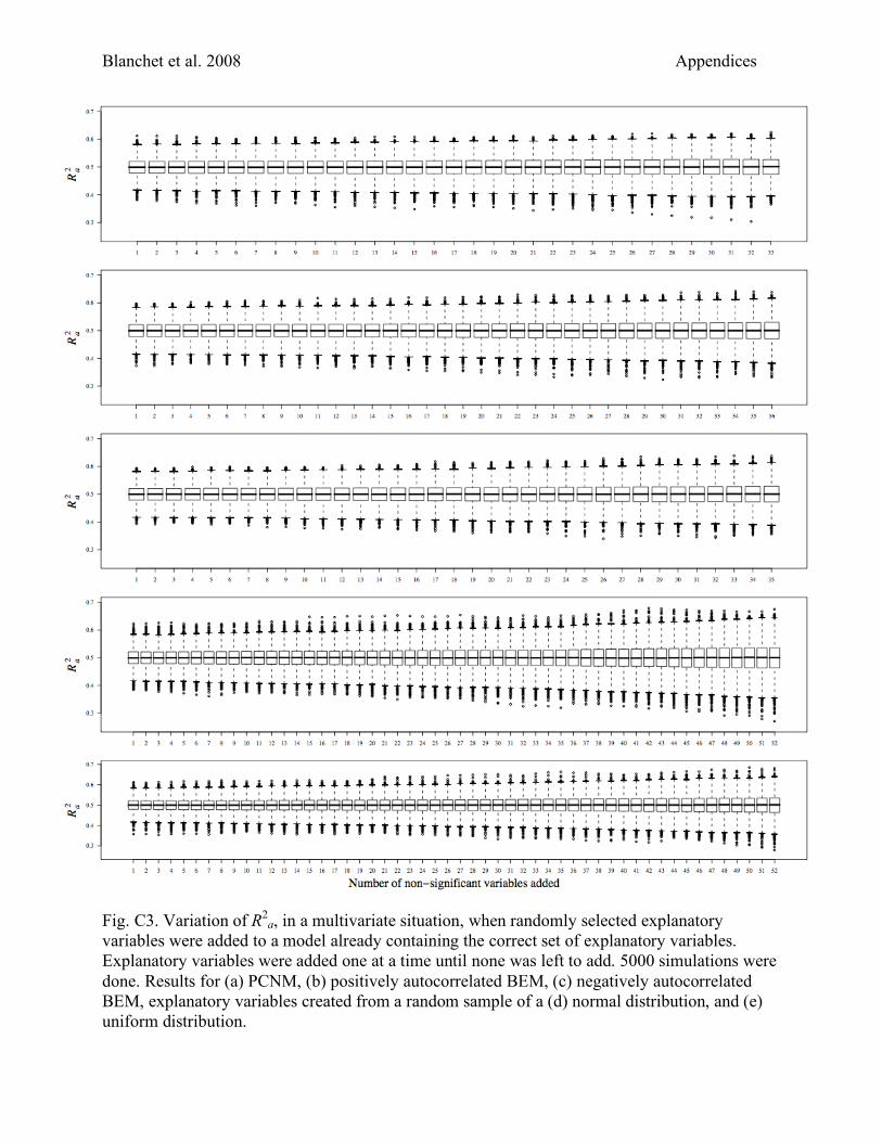
Simulations were also carried out in a multivariate

context. Response variables were constructed with the

same procedure as in the univariate situation, with a few

differences. Five response variables were constructed.

Each one was constructed based on three different

variables randomly sampled from the group of variables

under study (PCNM, BEM, normal, or uniform) with a

different set of random weights. The results, presented in

Appendix C, Fig. C3, lead to the same conclusions as in

the univariate situation.

In real cases, one does not know in advance which

explanatory variables are relevant. Given that the global

test was significant and a global R2a has been computed,

our second goal is now to prevent the selection from

being overly liberal. Preliminary simulations (not shown

here, but see Example: Bryce Canyon data below)

showed that, rather frequently, a forward selection run

on a globally significant model yielded a submodel

whose R2a was higher than the R2

a of the global model.

Obviously, this does not make sense. This problem was

also noticed by Cohen and Cohen (1983), as was

mentioned in Forward selection: a huge Type I error.

Therefore, the second message of this paper is the

following: forward selection should be carried out with

two stopping criteria: (1) the preselected significance

level alpha and (2) the R2a statistic of the global model.

We ran a new set of simulations to assess the

improvement brought by this second point. For

univariate simulations, we created response variables

using the same procedure as in the previous runs. This

was carried out for PCNM and BEM eigenfunctions and

non-orthogonal explanatory variables (normal and

uniform). Three variants were produced, differing by

the magnitude of the added error terms. The first set had

an error term equal to the standard deviation of the

deterministic portion of the response variable (as in the

previous simulations), the second set had an error with

standard deviation 25% that of the deterministic

portion, and the last set of simulations had a negligible

error term (0.001 times the standard deviation of the

deterministic portion). Each of these response variables

was submitted to the procedure above, i.e., a global test,

followed, if significant, by a forward selection of the

explanatory variables, using the two stopping criteria of

the last paragraph. Each result was compared to a result

obtained when only alpha was used as the stopping

criterion (as is usually done). Variables selected by

forward selection were compared to the variables chosen

to create the response variable. This was intended to

show how efficiently forward selection can identify the

correct set of explanatory variables.

Results for the simulations carried out with one

response variable and orthogonal predictors are pre-

sented in Fig. 4 (PCNM) and in Appendix D, Fig. D1

(BEM measuring positive autocorrelation) and Fig. D2

(BEM measuring negative autocorrelation). Since all

orthogonal predictor variables reacted in the same way,

Fig. 4 will be used in the discussion of all sets of

orthogonal variables.

When the error was equal to the standard deviation, a

forward selection done with the two stopping criteria (R2a

and alpha, Fig. 4a) rarely selected none or only one of

the variables used to create the response variables

(,1.5% of the times). Roughly 7.5% of the times, two

variables used to create the response variables were

selected. This percentage exceeded 20% for three

variables and 30% for four variables. In 37% of the

cases, all variables used to create the response were

found in the forward selection set. The positive influence

of the double stopping criterion is obvious when looking

at Fig. 4b: in .60% of the cases, no additional PCNM

eigenfunction was (incorrectly) selected.

FIG. 3. Variation of the adjusted coefficient of multiple determination (R2a ) when randomly selected principal coordinates of

neighbor matrices (PCNM) eigenfunctions were added to a model already containing the correct set of explanatory variables. ThePCNM eigenfunctions were added one at a time until none was left to add. Five thousand simulations were done. The upper andlower sections of the box represent the first (25%) and third quartiles (75%) of the data. The line in the middle of the box is themedian (50%). The lower whisker stands for the 1.5 interquartile range of the first quartile, and the upper whisker for the 1.5interquartile range of the third quartile. The points indicate outliers.


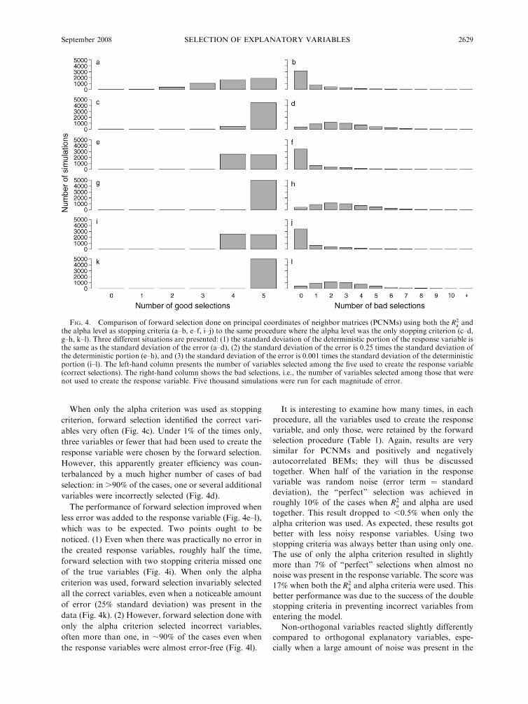
When only the alpha criterion was used as stopping

criterion, forward selection identified the correct vari-

ables very often (Fig. 4c). Under 1% of the times only,

three variables or fewer that had been used to create the

response variable were chosen by the forward selection.

However, this apparently greater efficiency was coun-

terbalanced by a much higher number of cases of bad

selection: in .90% of the cases, one or several additional

variables were incorrectly selected (Fig. 4d).

The performance of forward selection improved when

less error was added to the response variable (Fig. 4e–l),

which was to be expected. Two points ought to be

noticed. (1) Even when there was practically no error in

the created response variables, roughly half the time,

forward selection with two stopping criteria missed one

of the true variables (Fig. 4i). When only the alpha

criterion was used, forward selection invariably selected

all the correct variables, even when a noticeable amount

of error (25% standard deviation) was present in the

data (Fig. 4k). (2) However, forward selection done with

only the alpha criterion selected incorrect variables,

often more than one, in ;90% of the cases even when

the response variables were almost error-free (Fig. 4l).

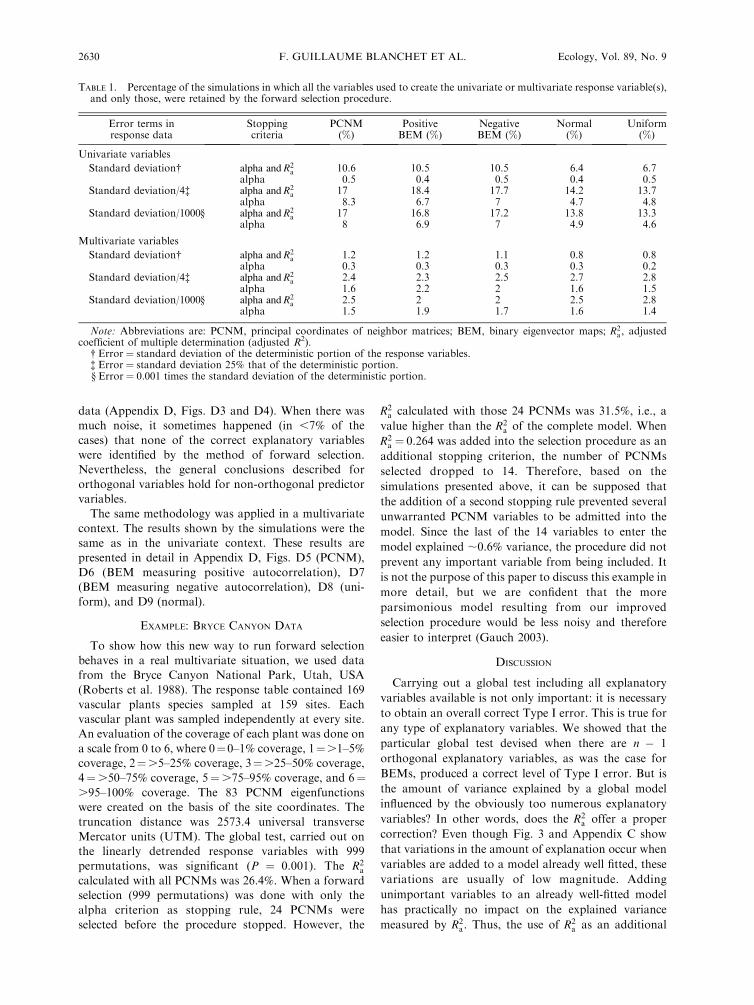
It is interesting to examine how many times, in each

procedure, all the variables used to create the response

variable, and only those, were retained by the forward

selection procedure (Table 1). Again, results are very

similar for PCNMs and positively and negatively

autocorrelated BEMs; they will thus be discussed

together. When half of the variation in the response

variable was random noise (error term ¼ standard

deviation), the ‘‘perfect’’ selection was achieved in

roughly 10% of the cases when R2a and alpha are used

together. This result dropped to ,0.5% when only the

alpha criterion was used. As expected, these results got

better with less noisy response variables. Using two

stopping criteria was always better than using only one.

The use of only the alpha criterion resulted in slightly

more than 7% of ‘‘perfect’’ selections when almost no

noise was present in the response variable. The score was

17% when both the R2a and alpha criteria were used. This

better performance was due to the success of the double

stopping criteria in preventing incorrect variables from

entering the model.

Non-orthogonal variables reacted slightly differently

compared to orthogonal explanatory variables, espe-

cially when a large amount of noise was present in the

FIG. 4. Comparison of forward selection done on principal coordinates of neighbor matrices (PCNMs) using both the R2a and

the alpha level as stopping criteria (a–b, e–f, i–j) to the same procedure where the alpha level was the only stopping criterion (c–d,g–h, k–l). Three different situations are presented: (1) the standard deviation of the deterministic portion of the response variable isthe same as the standard deviation of the error (a–d), (2) the standard deviation of the error is 0.25 times the standard deviation ofthe deterministic portion (e–h), and (3) the standard deviation of the error is 0.001 times the standard deviation of the deterministicportion (i–l). The left-hand column presents the number of variables selected among the five used to create the response variable(correct selections). The right-hand column shows the bad selections, i.e., the number of variables selected among those that werenot used to create the response variable. Five thousand simulations were run for each magnitude of error.


data (Appendix D, Figs. D3 and D4). When there was

much noise, it sometimes happened (in ,7% of the

cases) that none of the correct explanatory variables

were identified by the method of forward selection.

Nevertheless, the general conclusions described for

orthogonal variables hold for non-orthogonal predictor

variables.

The same methodology was applied in a multivariate

context. The results shown by the simulations were the

same as in the univariate context. These results are

presented in detail in Appendix D, Figs. D5 (PCNM),

D6 (BEM measuring positive autocorrelation), D7

(BEM measuring negative autocorrelation), D8 (uni-

form), and D9 (normal).

EXAMPLE: BRYCE CANYON DATA

To show how this new way to run forward selection

behaves in a real multivariate situation, we used data

from the Bryce Canyon National Park, Utah, USA

(Roberts et al. 1988). The response table contained 169

vascular plants species sampled at 159 sites. Each

vascular plant was sampled independently at every site.

An evaluation of the coverage of each plant was done on

a scale from 0 to 6, where 0¼0–1% coverage, 1¼.1–5%

coverage, 2¼.5–25% coverage, 3¼.25–50% coverage,

4¼.50–75% coverage, 5¼.75–95% coverage, and 6¼.95–100% coverage. The 83 PCNM eigenfunctions

were created on the basis of the site coordinates. The

truncation distance was 2573.4 universal transverse

Mercator units (UTM). The global test, carried out on

the linearly detrended response variables with 999

permutations, was significant (P ¼ 0.001). The R2a

calculated with all PCNMs was 26.4%. When a forward

selection (999 permutations) was done with only the

alpha criterion as stopping rule, 24 PCNMs were

selected before the procedure stopped. However, the

R2a calculated with those 24 PCNMs was 31.5%, i.e., a

value higher than the R2a of the complete model. When

R2a ¼ 0.264 was added into the selection procedure as an

additional stopping criterion, the number of PCNMs

selected dropped to 14. Therefore, based on the

simulations presented above, it can be supposed that

the addition of a second stopping rule prevented several

unwarranted PCNM variables to be admitted into the

model. Since the last of the 14 variables to enter the

model explained ;0.6% variance, the procedure did not

prevent any important variable from being included. It

is not the purpose of this paper to discuss this example in

more detail, but we are confident that the more

parsimonious model resulting from our improved

selection procedure would be less noisy and therefore

easier to interpret (Gauch 2003).

DISCUSSION

Carrying out a global test including all explanatory

variables available is not only important: it is necessary

to obtain an overall correct Type I error. This is true for

any type of explanatory variables. We showed that the

particular global test devised when there are n � 1

orthogonal explanatory variables, as was the case for

BEMs, produced a correct level of Type I error. But is

the amount of variance explained by a global model

influenced by the obviously too numerous explanatory

variables? In other words, does the R2a offer a proper

correction? Even though Fig. 3 and Appendix C show

that variations in the amount of explanation occur when

variables are added to a model already well fitted, these

variations are usually of low magnitude. Adding

unimportant variables to an already well-fitted model

has practically no impact on the explained variance

measured by R2a . Thus, the use of R2

a as an additional

TABLE 1. Percentage of the simulations in which all the variables used to create the univariate or multivariate response variable(s),and only those, were retained by the forward selection procedure.

Error terms inresponse data

Stoppingcriteria

PCNM(%)

PositiveBEM (%)

NegativeBEM (%)

Normal(%)

Uniform(%)

Univariate variables

Standard deviation� alpha and R2a 10.6 10.5 10.5 6.4 6.7

alpha 0.5 0.4 0.5 0.4 0.5Standard deviation/4� alpha and R2

a 17 18.4 17.7 14.2 13.7alpha 8.3 6.7 7 4.7 4.8

Standard deviation/1000§ alpha and R2a 17 16.8 17.2 13.8 13.3

alpha 8 6.9 7 4.9 4.6

Multivariate variables

Standard deviation� alpha and R2a 1.2 1.2 1.1 0.8 0.8

alpha 0.3 0.3 0.3 0.3 0.2Standard deviation/4� alpha and R2

a 2.4 2.3 2.5 2.7 2.8alpha 1.6 2.2 2 1.6 1.5

Standard deviation/1000§ alpha and R2a 2.5 2 2 2.5 2.8

alpha 1.5 1.9 1.7 1.6 1.4

Note: Abbreviations are: PCNM, principal coordinates of neighbor matrices; BEM, binary eigenvector maps; R2a , adjusted

coefficient of multiple determination (adjusted R2).� Error¼ standard deviation of the deterministic portion of the response variables.� Error¼ standard deviation 25% that of the deterministic portion.§ Error¼ 0.001 times the standard deviation of the deterministic portion.


stopping criterion is a good choice in a forward selection

procedure.

Freedman et al. (1992) suggested a procedure close to

ours. They proposed to use an estimate of the residual

variance calculated with all explanatory variables as the

stopping criterion in forward selection. Their proposi-

tion is based on a mathematical demonstration showing

that the residual variance can be found theoretically for

any subset of variables. They concluded by saying that

any consistent estimator of the residual variance can be

a good stopping criterion, meaning that it should

preserve the nominal significance level. We have shown,

with the help of simulations, that this is true only if the

residual variance is corrected, as is the case for R2a .

The use of our double stopping rule (R2a combined

with alpha level) has a number of impacts on the final

selection. The most important is that selection of useless

variables occurs less often. There are fewer variables

selected and the selection is more realistic. However,

Neter et al. (1996: Chapter 8) commented that the use of

automatic selection procedures may lead to the selection

of a set of variables that is not the best but is very

suitable for the response variable under study. Our new

approach does not prevent such outcomes; it prevents

the possibility of overexplaining response variables by a

set of ‘‘too-well-chosen’’ explanatory variables. The use

of R2a in addition to the alpha criterion for the stopping

procedure was shown, however, to select the best model

more often (Fig. 4 and Appendix D).

Neter et al. (1996: Chapter 8) proposed other

parameters that could be used as stopping criteria: the

total mean square error and the prediction sum of

squares. We decided to use the R2a because it offers the

advantage of being an unbiased estimate of the amount

of explained variance. Also, this parameter is well-

known by ecologists, which is not the case for the other

two proposed by Neter et al. (1996).

Various attempts have been published to try to correct

for the overestimation of R2 that forward selection is

known to generate. Diehr and Hoflin (1974), followed

by Wilkinson (1979), Rencher and Pun (1980), and

Wilkinson and Dallal (1981), tried to correct the

variance, measured by R2, when a subset of explanatory

variables is sampled from a multiple regression, but the

solutions proposed by these authors are still biased.

Copas and Long (1991) proposed to correct for the

overfitting of the response by using an empirical

Bayesian criterion. Their method is interesting but

restrictive: the explanatory variables need to be orthog-

onal and the response variable normal.

Westfall et al. (1998) tried to solve the problem by

using a Bonferroni correction on the calculated P values.

We compared that approach with ours and realized that

it is well suited for saturated or supersaturated designs.

However, when there are fewer variables than the

number of sites, correcting the P values still leaves us

with an overestimated proportion of explained variance.

Another major drawback of all these approaches is that

they do not consider the multivariate situation. Fur-

thermore, stepwise corrections of P values lead to an

undefined overall level of Type I error.

The R package ‘‘packfor’’ contains two functions to

perform forward selection based upon a permutation

and a parametric test. It contains all the new improve-

ments presented in this paper.

The conclusions reached in this study are based on

simulations. We tried to make the simulations as general

as possible, even though we did not simulate all possible

types of ecological data. This is always the case in

simulation studies (Milligan 1996). Hurlbert’s unicorns

(Hurlbert 1990) provide a good example of how peculiar

ecological data can be.

ACKNOWLEDGMENTS

We thank Dave Roberts for permission to use the BryceCanyon data to illustrate the method presented in this paper.This research was supported by NSERC grant number 7738 toP. Legendre.

LITERATURE CITED

Anderson, M. J., and P. Legendre. 1999. An empiricalcomparison of permutation methods for tests of partialregression coefficients in a linear model. Journal of StatisticalComputation and Simulation 62:271–303.

Bellier, E., P. Monestiez, J.-P. Durbec, and J.-N. Candau. 2007.Identifying spatial relationships at multiple scales: principalcoordinates of neighbour matrices (PCNM) and geostatis-tical approaches. Ecography 3:385–399.

Bonferroni, C. E. 1935. Il calcolo delle assicurazioni su gruppidi teste. Pages 13–60 in Studi in onore del ProfessoreSalvatore Ortu Carboni. Rome, Italy.

Borcard, D., and P. Legendre. 2002. All-scale spatial analysis ofecological data by means of principal coodinates ofneighbour matrices. Ecological Modelling 153:51–68.

Borcard, D., P. Legendre, C. Avois-Jacquet, and H. Tuosimo-to. 2004. Dissecting the spatial structure of ecological data atmultiple scales. Ecology 85:1826–1832.

Brind’Amour, A., D. Boisclair, P. Legendre, and D. Borcard.2005. Multiscale spatial distribution of a littoral fishcommunity in relation to environmental variables. Limnol-ogy and Oceanography 50:465–479.

Chatterjee, S., and B. Price. 1977. Regression analysis byexample. Wiley, New York, New York, USA.

Cohen, J., and P. Cohen. 1983. Applied multiple regression/correlation analysis for the behavioral sciences. LawrenceErlbaum, Hillsdale, New Jersey, USA.

Copas, J. B., and T. Long. 1991. Estimating the residualvariance in orthogonal regression with variable selection.Statistician 40:51–59.

Derksen, S., and H. J. Keselman. 1992. Backward, forward andstepwise automated subset selection algorithms: frequency ofobtaining authentic and noise variables. British Journal ofMathematical and Statistical Psychology 45:262–282.

Diehr, G., and D. R. Hoflin. 1974. Approximating thedistribution of the sample R2 in best subset regressions.Technometrics 16:317–320.

Dray, S., P. Legendre, and P. R. Peres-Neto. 2006. Spatialmodelling: a comprehensive framework for principal coordi-nate analysis of neighbour matrices (PCNM). EcologicalModelling 196:483–493.

Duque, A. J., J. F. Duivenvoorden, J. Cavelier, M. Sanchez, C.Polania, and A. Leon. 2005. Ferns and Melastomataceae asindicators of vascular plant composition in rain forests ofColombian Amazonia. Plant Ecology 178:1–13.


Ezekiel, M. 1930. Method of correlation analysis. John Wileyand Sons, New York, New York, USA.

Fisher, R. A. 1935. The design of experiments. Oliver and Boyd,Edinburgh, UK.

Freedman, L. S., D. Pee, and D. N. Midthune. 1992. Theproblem of underestimating the residual error variance inforward stepwise regression. Statistician 41:405–412.

Gauch, H. G. 1993. Prediction, parsimony and noise. AmericanScientist 81:468–478.

Gauch, H. G. 2003. Scientific method in practice. CambridgeUniversity Press, New York, New York, USA.

Halpern, B. S., and K. Cottenie. 2007. Little evidence forclimate effects on local-scale structure and dynamics ofCalifornia kelp forest communities. Global Change Biology13:236–251.

Hurlbert, S. H. 1990. Spatial-distribution of the montaneunicorn. Oikos 58:257–271.

Legendre, P., and L. Legendre. 1998. Numerical ecology.Second English edition. Elsevier, Amsterdam, The Nether-lands.

Manly, B. F. J. 1997. Randomization, bootstrap and MonteCarlo methods in biology. Second edition. Chapman andHall, London, UK.

Miller, J. K. 1975. The sampling distribution and a test for thesignificance of the bimultivariate redundancy statistic: aMonte Carlo study. Multivariate Behavioral Research 10:233–244.

Milligan, G. W. 1996. Clustering validation: results andimplications for applied analyses. Pages 341–375 in P. Arabie,L. J. Hubert, and G. De Soet, editors. Clustering andclassification. World Scientific, River Edge, New Jersey,USA.

Neter, J., M. H. Kutner, C. J. Nachtsheim, and W. Wasserman.1996. Applied linear statistical models. Fourth edition. Irwin,Chicago, Illinois, USA.

Ohtani, K. 2000. Bootstrapping R2 and adjusted R2 inregression analysis. Economic Modelling 17:473–483.

Pitman, E. J. G. 1937a. Significance tests which may be appliedto samples from any populations. Journal of the RoyalStatistical Society 4(Supplement):119–130.

Pitman, E. J. G. 1937b. Significance tests which may be appliedto samples from any populations. II. The correlation

coefficient test. Journal of the Royal Statistical Society4(Supplement):225–232.

Pitman, E. J. G. 1938. Significance tests which may be appliedto samples from any populations. III. The analysis ofvariance test. Biometrika 29:322–335.

Rencher, A. C., and F. C. Pun. 1980. Inflation of R2 in bestsubset regression. Technometrics 22:49–53.

Roberts, D. W., D. Wight, G. P Hallsten, and D. Betz. 1988.Plant community distribution and dynamics in Bryce CanyonNational Park. Final Report PX 1200-7-0966. United StatesDepartment of Interior, National Park Service, Washington,D.C., USA.

Sidak, Z. 1967. Rectangular confidence regions for the means ofmultivariate normal distributions. Journal of the AmericanStatistical Association 62:626–633.

Telford, R. J., and H. J. B. Birks. 2005. The secret assumptionof transfer functions: problems with spatial autocorrelationin evaluating model performance. Quaternary ScienceReviews 24:2173–2179.

ter Braak, C. J. F. 1988. CANOCO—a FORTRAN programfor canonical community ordination by [partial] [detrended][canonical] correspondence analysis, principal componentanalysis and redundancy analysis. Version 2.1. AgriculturalMathematics Group, Ministry of Agriculture and Fisheries,Wageningen, The Netherlands.

Thioulouse, J., D. Chessel, and S. Champely. 1995. Multivar-iate analysis of spatial patterns: a unified approach to localand global structures. Environmental and Ecological Statis-tics 2:1–14.

Westfall, P. H., S. S. Young, and D. K. J. Lin. 1998. Forwardselection error control in the analysis of supersaturateddesigns. Statistica Sinica 8:101–117.

Whittingham, M. J., P. A. Stephens, R. B. Bradbury, and R. P.Freckleton. 2006. Why do we still use stepwise modelling inecology and behaviour? Journal of Animal Ecology 75:1182–1189.

Wilkinson, L. 1979. Test of significance in stepwise regression.Psychological Bulletin 86:168–174.

Wilkinson, L., and G. E. Dallal. 1981. Tests of significance inforward selection regression with an F-to-enter stopping rule.Technometrics 23:377–380.

APPENDIX A

Forward selection simulations carried out in the multivariate situation: Type I error (Ecological Archives E089-147-A1).

APPENDIX B

Selection of individual variables by classical forward selection in the multivariate situation (Ecological Archives E089-147-A2).

APPENDIX C

Forward selection simulations carried out in the multivariate situation: variation of R2a when randomly selected variables are

added to a model (Ecological Archives E089-147-A3).

APPENDIX D

Forward selection simulations carried out in the multivariate situation: using one or two stopping criteria (Ecological ArchivesE089-147-A4).


Blanchet et al. 2008 Appendices

APPENDIX A

Ecological Archives E089-147-A1

FORWARD SELECTION SIMULATIONS CARRIED OUT IN THE MULTIVARIATE SITUATION: TYPE I ERROR. ONE FIGURE (FIG. A1)

Fig. A1. Results of 5000 forward selection simulations when alpha was the only criterion used as a stopping criterion. The five response variables were random normal; they were unrelated to the explanatory variables. (a) Boxplots of R2

a values calculated for each of the four sets of explanatory variables: PCNM, BEM, normal, and uniform. (b) Number of PCNMs selected by forward selection. (c) Number of BEMs selected by forward selection. (d) Number of uniform variables selected by forward selection. (e) Number of normal variables selected by forward selection.


APPENDIX B


SELECTION OF INDIVIDUAL VARIABLES BY CLASSICAL FORWARD SELECTION IN THE MULTIVARIATE SITUATION. ONE FIGURE (FIG. B1)

Fig. B1. Details on the type I error of the classical forward selection procedure, using the alpha-level as the only stopping criterion: number of times each spatial variable was selected after 5000 simulations. (a) Results for PCNMs. (b) Results for BEMs.


APPENDIX C


FORWARD SELECTION SIMULATIONS CARRIED OUT IN THE MULTIVARIATE SITUATION: VARIATION OF R2a WHEN RANDOMLY SELECTED VARIABLES ARE ADDED TO A MODEL.

THREE FIGURES (FIGS. C1, C2, C3) Fig. C1. Variation of R2

a when randomly selected BEM eigenfunctions were added to a model already containing the correct set of explanatory variables. BEM eigenfunctions were added one at a time until none was left to add. 5000 simulations were done. (a) Results for positively autocorrelated BEM eigenfunctions. (b) Results for negatively autocorrelated BEM eigenfunctions.


Fig. C2. Variation of R2

a when randomly selected non-orthogonal explanatory variables were added to a model already containing the correct set of explanatory variables. Non-orthogonal explanatory variables were added one at a time until none was left to add. 5000 simulations were done. Results for explanatory variables created from a random sample of a (a) normal distribution and (b) uniform distribution.


Fig. C3. Variation of R2

a, in a multivariate situation, when randomly selected explanatory variables were added to a model already containing the correct set of explanatory variables. Explanatory variables were added one at a time until none was left to add. 5000 simulations were done. Results for (a) PCNM, (b) positively autocorrelated BEM, (c) negatively autocorrelated BEM, explanatory variables created from a random sample of a (d) normal distribution, and (e) uniform distribution.


APPENDIX D


FORWARD SELECTION SIMULATIONS CARRIED OUT IN THE MULTIVARIATE SITUATION: USING ONE OR TWO STOPPING CRITERIA. NINE FIGURES (FIGS. D1, D2, D3, D4, D5, D6, D7, D8, D9)

Fig. D1. Comparison of forward selection done on positively autocorrelated BEMs using both the R2a and the alpha-level as stopping criteria (a-b, e-f, i-j), to the same procedure where the alpha-

level was the only stopping criterion (c-d, g-h, k-l). Three different situations are presented: (1) the standard deviation of the deterministic portion of the response variable is the same as the standard deviation of the error (a-d), (2) the standard deviation of the error is 0.25 times the standard deviation of the deterministic portion (e-h), and (3) the standard deviation of the error is 0.001 times the standard deviation of the deterministic portion (i-l). The left-hand column presents the number of variables selected among the five used to create the response variable (correct selections). The right-hand column shows the bad selections, i.e., the number of variables selected among those that were not used to create the response variable. 5000 simulations were run for each magnitude of error. This set of figures presents results for the univariate situation.


Fig. D2. Comparison of forward selection done on negatively autocorrelated BEMs using both the R2

a and the alpha-level as stopping criteria (a-b, e-f, i-j), to the same procedure where the alpha-level was the only stopping criterion (c-d, g-h, k-l). Three different situations are presented: (1) the standard deviation of the deterministic portion of the response variable is the same as the standard deviation of the error (a-d), (2) the standard deviation of the error is 0.25 times the standard deviation of the deterministic portion (e-h), and (3) the standard deviation of the error is 0.001 times the standard deviation of the deterministic portion (i-l). The left-hand column presents the number of variables selected among the five used to create the response variable (correct selections). The right-hand column shows the bad selections, i.e., the number of variables selected among those that were not used to create the response variable. 5000 simulations were run for each magnitude of error. This set of figures presents results for the univariate situation.


Fig. D3. Comparison of forward selection done on variables randomly selected from a normal distribution using both the R2



Fig. D4. Comparison of forward selection done on variables randomly selected from a uniform distribution using both the R2



Fig. D5. Comparison of forward selection done on PCNMs using both the R2

a and the alpha-level as stopping criteria (a-b, e-f, i-j), to the same procedure where the alpha-level was the only stopping criterion (c-d, g-h, k-l). Three different situations are presented: (1) the standard deviation of the deterministic portion of the response variable is the same as the standard deviation of the error (a-d), (2) the standard deviation of the error is 0.25 times the standard deviation of the deterministic portion (e-h), and (3) the standard deviation of the error is 0.001 times the standard deviation of the deterministic portion (i-l). The left-hand column presents the number of variables selected among the five used to create the response variable (correct selections). The right-hand column shows the bad selections, i.e., the number of variables selected among those that were not used to create the response variable. 5000 simulations were run for each magnitude of error. This set of figures presents results for the multivariate situation.


Fig. D6. Comparison of forward selection done on positively autocorrelated BEMs using both the R2a and the alpha-level as stopping criteria (a-b, e-f, i-j), to the same procedure where the alpha-

level was the only stopping criterion (c-d, g-h, k-l). Three different situations are presented: (1) the standard deviation of the deterministic portion of the response variable is the same as the standard deviation of the error (a-d), (2) the standard deviation of the error is 0.25 times the standard deviation of the deterministic portion (e-h), and (3) the standard deviation of the error is 0.001 times the standard deviation of the deterministic portion (i-l). The left-hand column presents the number of variables selected among the five used to create the response variable (correct selections). The right-hand column shows the bad selections, i.e., the number of variables selected among those that were not used to create the response variable. 5000 simulations were run for each magnitude of error. This set of figures presents results for the multivariate situation.


Fig. D7. Comparison of forward selection done on negatively autocorrelated BEMs using both the R2



Fig. D8. Comparison of forward selection done on variables randomly selected from a normal distribution using both the R2



Fig. D9. Comparison of forward selection done on variables randomly selected from a uniform distribution using both the R2


FORWARD SELECTION OF EXPLANATORY VARIABLES

Documents

Transcript of FORWARD SELECTION OF EXPLANATORY VARIABLES