1

Multiple Regression Response, Y (numerical) Explanatory variables, X1,

X2, …Xk (numerical) New explanatory variables

can be created from existing explanatory variables.

2

Home gas consumption Weekly gas consumption for a

home in England. Average outside temperature. There are 26 weeks before

insulation was added and 18 weeks after adding insulation.

3

Home gas consumption Response: Gas – gas

consumption in 1000’s of cubic feet.

Explanatory: Temp – average outside temperature in oC.

4

Home gas consumption Response: Gas – gas consumption

in 1000’s of cubic feet. Explanatory: Insul – a dummy or

indicator variable Insul = 0, before insulation was

added Insul =1, after insulation was added

5

2

3

4

5

6

7

8

Gas

-5 0 5 10 15

Temp

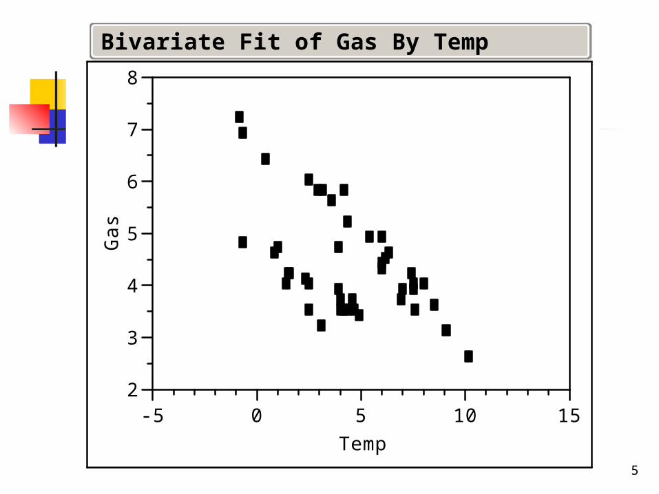
Bivariate Fit of Gas By Temp

6

General Trend As outside temperature

increases, gas consumption goes down.

There is something funny about the plot.

7

2

3

4

5

6

7

8

Gas

-5 0 5 10 15

Temp

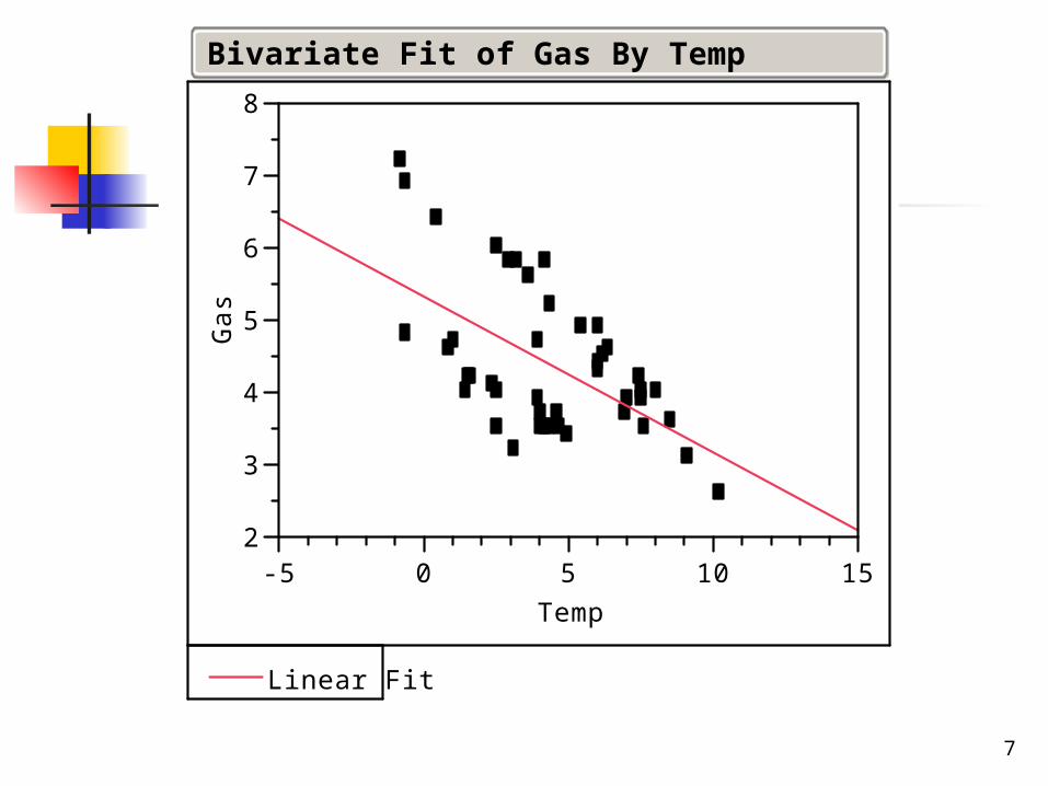
Linear Fit

Bivariate Fit of Gas By Temp

8

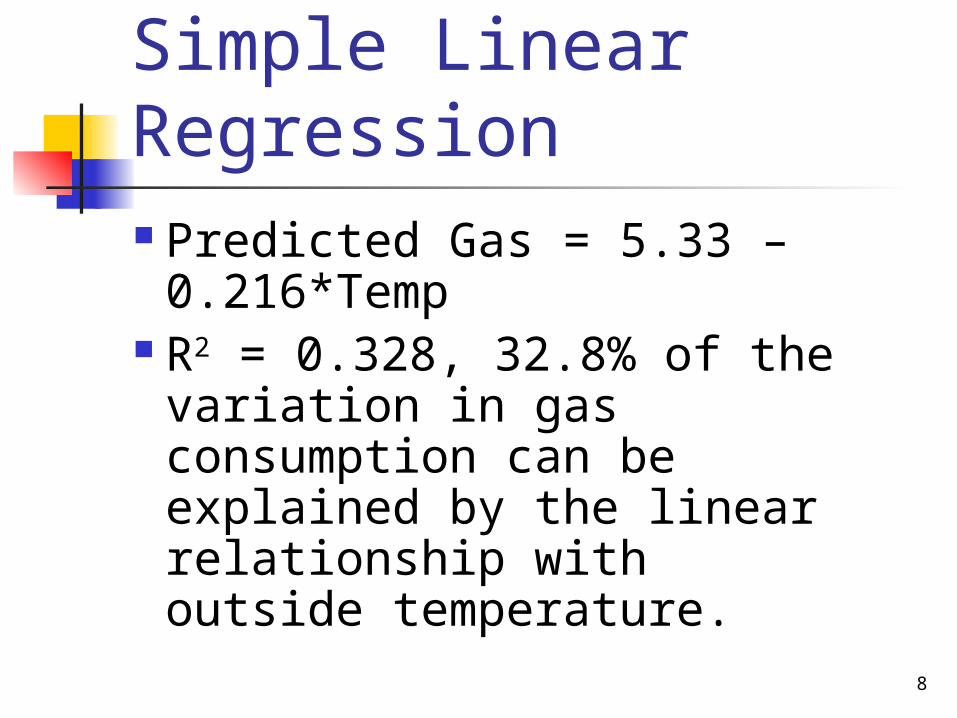
Simple Linear Regression Predicted Gas = 5.33 –

0.216*Temp R2 = 0.328, 32.8% of the

variation in gas consumption can be explained by the linear relationship with outside temperature.

9

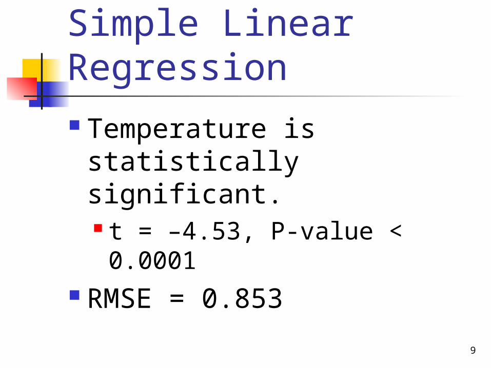
Simple Linear Regression Temperature is

statistically significant. t = –4.53, P-value < 0.0001

RMSE = 0.853

10

-2.0

-1.5

-1.0

-0.5

0.0

0.5

1.0

1.5

2.0

Res

idua

l

-5 0 5 10 15

Temp

11

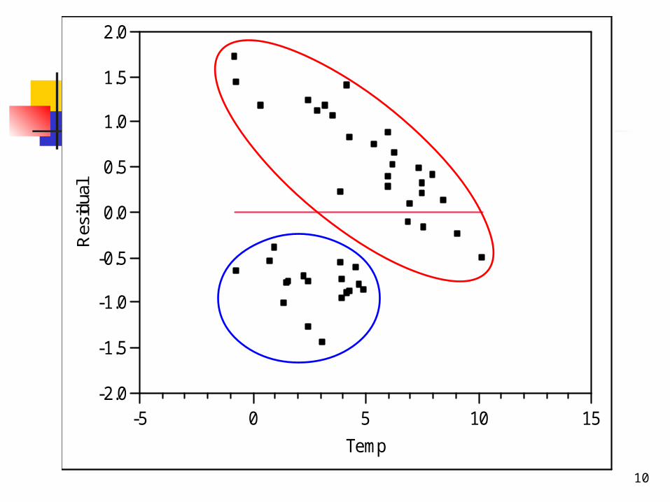
Plot of Residuals The plot of residuals versus

temperature does not appear to be a random scatter.

There appears to be two groups of values.

12

How can we do better? If the two groups in the

residual plot are associated with data from the un-insulated and insulated house, adding the dummy (indicator) variable Insul can explain more of the variation in gas consumption.

13

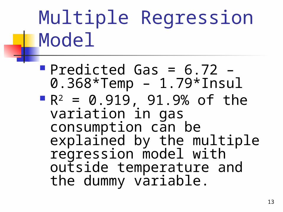
Multiple Regression Model Predicted Gas = 6.72 –

0.368*Temp – 1.79*Insul R2 = 0.919, 91.9% of the

variation in gas consumption can be explained by the multiple regression model with outside temperature and the dummy variable.

14

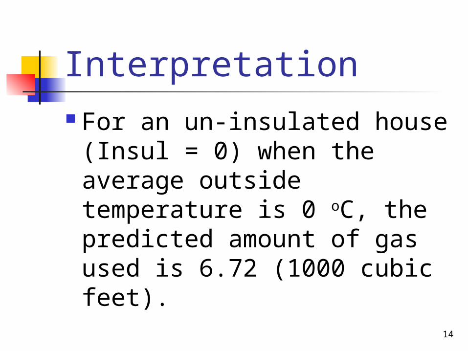
Interpretation For an un-insulated house

(Insul = 0) when the average outside temperature is 0 oC, the predicted amount of gas used is 6.72 (1000 cubic feet).

15

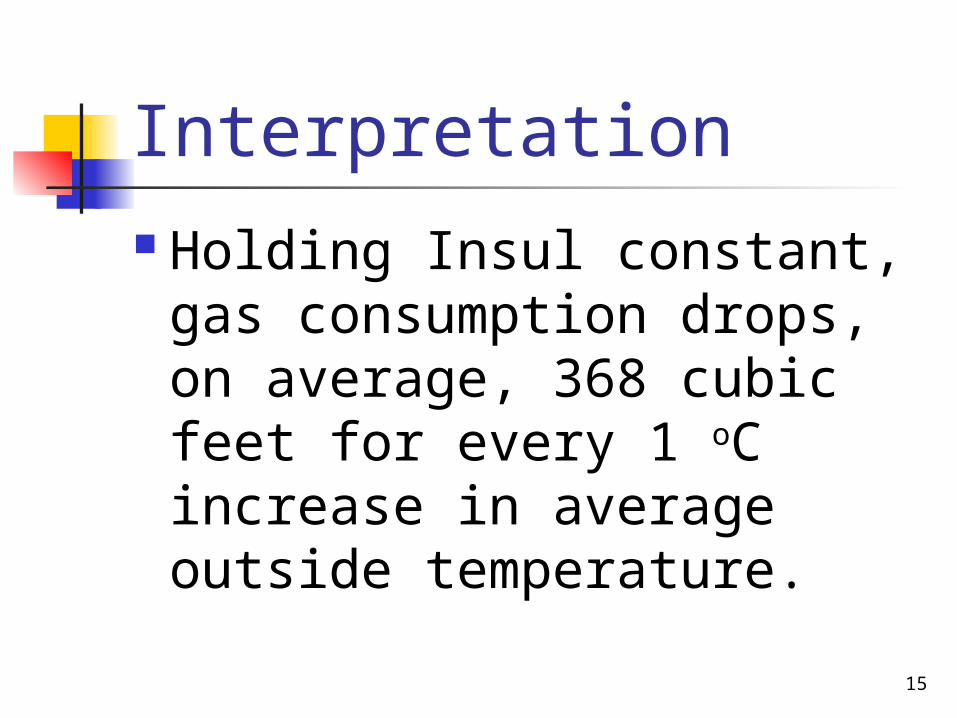
Interpretation Holding Insul constant, gas

consumption drops, on average, 368 cubic feet for every 1 oC increase in average outside temperature.

16

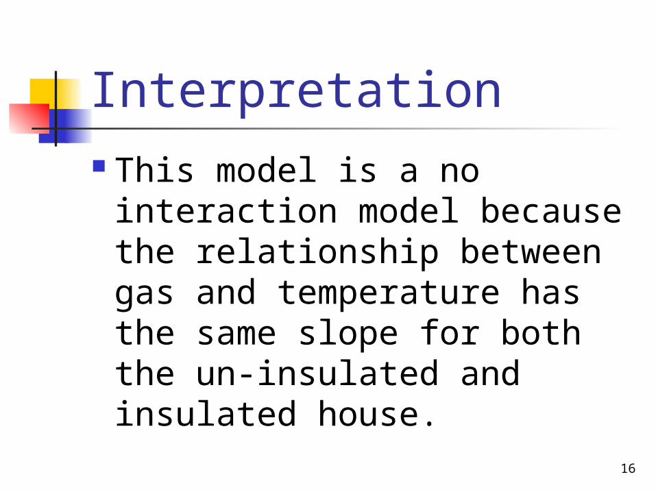
Interpretation This model is a no

interaction model because the relationship between gas and temperature has the same slope for both the un-insulated and insulated house.

17

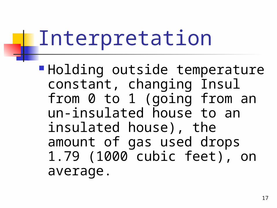
Interpretation Holding outside temperature

constant, changing Insul from 0 to 1 (going from an un-insulated house to an insulated house), the amount of gas used drops 1.79 (1000 cubic feet), on average.

18

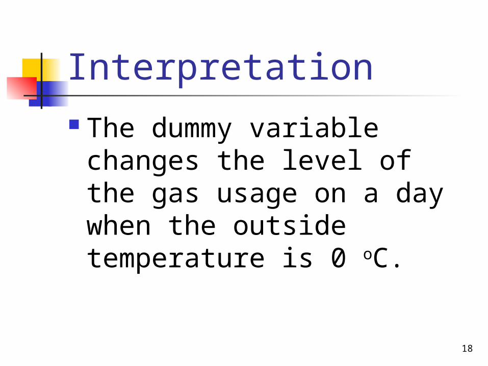
Interpretation The dummy variable

changes the level of the gas usage on a day when the outside temperature is 0 oC.

19

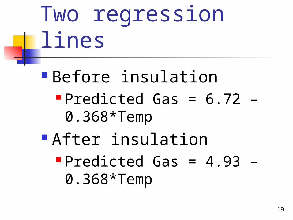
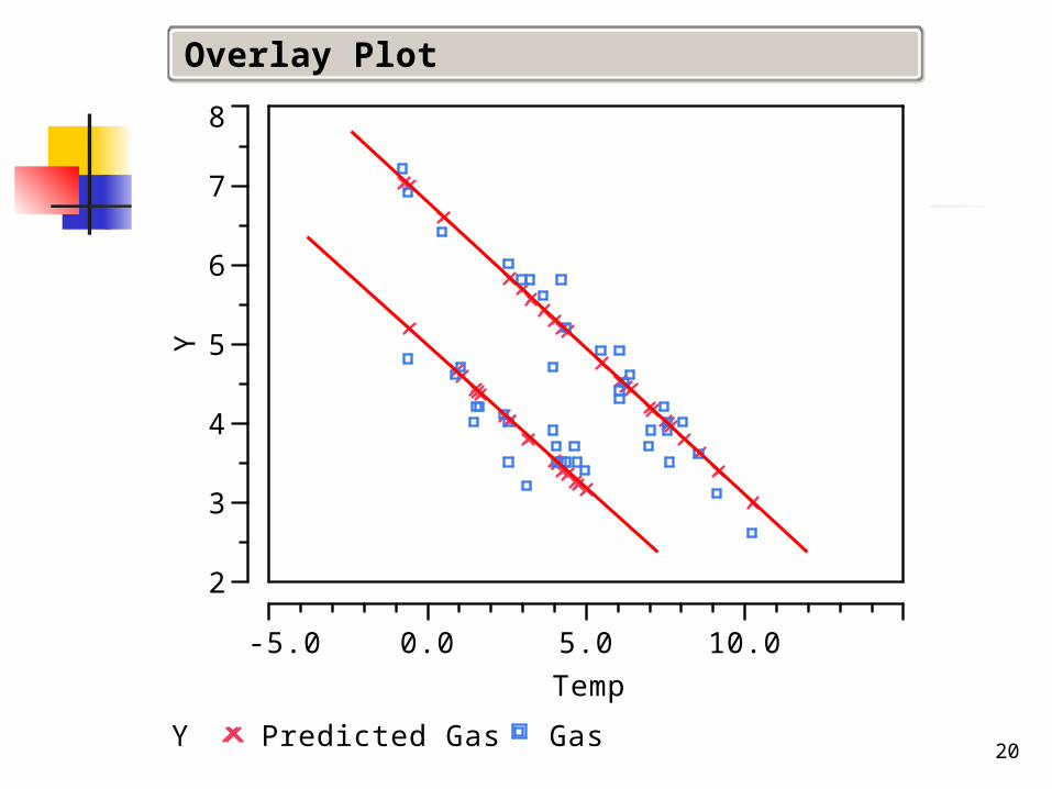
Two regression lines Before insulation

Predicted Gas = 6.72 – 0.368*Temp

After insulation Predicted Gas = 4.93 – 0.368*Temp

20

2

3

4

5

6

7

8

Y

-5.0 0.0 5.0 10.0

Temp

Overlay Plot

Y Predicted Gas Gas

21

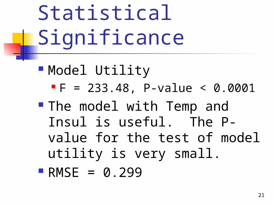
Statistical Significance Model Utility

F = 233.48, P-value < 0.0001 The model with Temp and Insul

is useful. The P-value for the test of model utility is very small.

RMSE = 0.299

22

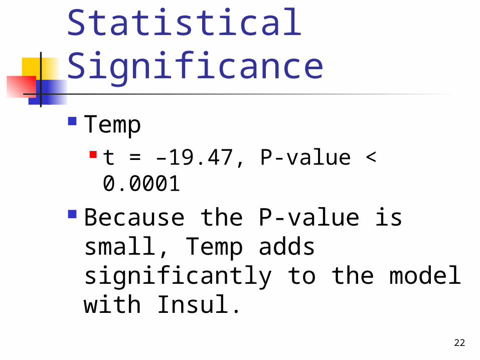
Statistical Significance Temp

t = –19.47, P-value < 0.0001 Because the P-value is

small, Temp adds significantly to the model with Insul.

23

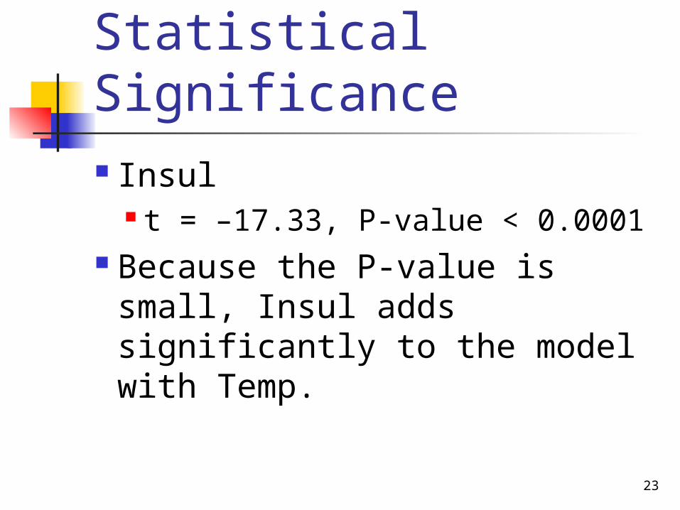
Statistical Significance Insul

t = –17.33, P-value < 0.0001 Because the P-value is small,

Insul adds significantly to the model with Temp.

24

-1

-0.5

0

0.5

1

No

Inte

ract

ion

Res

idua

l

-5 0 5 10 15

Temp

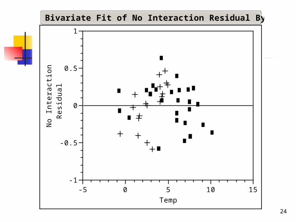
Bivariate Fit of No Interaction Residual By Temp