Forensic Tracking and Mobility Prediction in Vehicular...

Chapter 21

FORENSIC TRACKING ANDMOBILITY PREDICTION INVEHICULAR NETWORKS

Saif Al-Kuwari and Stephen Wolthusen

Abstract Most contemporary tracking applications consider an online approachwhere the target is tracked in real time. In criminal investigations,however, it is often the case that only offline tracking is possible, i.e.,tracking takes place after the fact. In offline tracking, given an incom-plete trace of a target, the task is to reconstruct the missing parts andobtain the full trace. The proliferation of modern transportation sys-tems means that a targeted entity is likely to use multiple modes oftransportation. This paper introduces a class of mobility models tai-lored for forensic analysis. The mobility models are used to constructa multi-modal forensic tracking system that can reconstruct a completetrace of a target. Theoretical analysis of the reconstruction algorithmdemonstrates that it is both complete and optimal.

Keywords: Forensic tracking, mobility models, trace reconstruction

1. Introduction

Traditional digital forensics is primarily concerned with extractingevidence from electronic devices that may have been associated with orused in criminal activities. In most criminal cases, however, it is alsodesirable to uncover additional information about suspects, includingdetails about their physical activities. Investigating the locations of asuspect before, during and after a crime, may constitute key evidence,especially if it helps prove that the suspect was in a specific location ata specific time that he previously denied. This type of investigation iscalled “forensic tracking” [2], where the tracking is conducted for forensicpurposes.

304 ADVANCES IN DIGITAL FORENSICS VIII

Forensic tracking investigations are usually carried out in an offlinemanner. A location trace of a suspect is obtained, which undergoes aprobabilistic analysis designed to reconstruct the missing parts. A primeexample is when a target is randomly captured by CCTV cameras scat-tered over a particular area. Previous work has focused on conductingoffline forensic investigations in a vehicular setting [1]. This paper ex-tends the approach to deal with scenarios where a suspect uses multiplemodes of transportation.

The trace reconstruction algorithm described in this paper involvestwo main phases: (i) scene representation; and (ii) trace reconstruction.Scene representation uses information about when and where a targetwas observed to create scattered points over an area, that are subse-quently connected to determine the routes that the target could havetaken. Trace reconstruction attempts to fill the gaps of missing databetween the points where the target was observed. In a multi-modalscenario, a targeted entity is expected to use multiple modes of trans-portation; thus, all possible routes through the gaps involving pedestrianroutes, public routes and a combination of both must be considered toobtain a complete trace of the target. Theoretical analysis of the recon-struction algorithm demonstrates that it is both complete and optimal.

2. Scene Representation

In order to systematically reconstruct the trace of a target, a graph-ical representation (map) of the crime scene and the surrounding areamust be generated. This is accomplished in five steps as described inthis section. To simplify the notation, unnecessary labels and tags aredropped when referring to certain edges and vertices in the map.

Step 1: Map Preparation. In this initial step, a schematic map GM

(based on a geographical area M) of the reconstruction scene is obtained.The reconstruction scene corresponds to the area over which the targettrace is to be reconstructed. No restrictions are imposed on the size ofGM other than it must cover: (i) all the points at which the target wasobserved (available traces of the target); and (ii) crime location(s).

Let GM = (VGM , EGM ) be a scene graph with vertices VGM and edgesEGM . We assume that {XGM

s ∪CGM} ∈ VGM such that:

XGMs = {xκp

1 , . . . , xκqn } is the set of locations where the target s was

observed; κp < κq are the first and last times that s was observedin GM .

CGM = {cκk1 , . . . , cκl

m} is the set of crime locations visited betweentimes k and l. To simplify the discussion, we describe the specifics

Al-Kuwari & Wolthusen 305

of the reconstruction algorithm using a single crime. Of course,the algorithm is applicable to multiple crimes.

Step 2: Route Marking. In this step, relevant public transportnetworks (e.g., buses and trains) B1, B1, . . . , Bn ∈ B are marked onGM . A transport network Bj ∈ B consists of a set of routes Bj =

{RBj

1 , RBj

2 , . . . , RBjr } that constitute most of the vertices and edges in

GM . Since only public transport routes are marked, vertices in a routeRi correspond to a stop (e.g., train station) denoted as an S-vertex, ora road turn denoted as a U -vertex. Similarly, edges can be routed (i.e.,part of a route) denoted as a B-edge, or unrouted denoted as a W -edge(mostly added in Step 4 below).

Let eρ be an edge of type ρ, then:

ρ =

!

B if e ∈"

Bj∈B

"|Bj |i=1 R

Bj

i

W if e ∈ EGM \"

Bj∈B

"|Bj |i=1 R

Bj

i

where |x| is the number of elements in set x assuming that x does nothave repeated elements (i.e., corresponding to loop-free routes).

Thus, a route Ri is defined by the set of vertices VRi = {v1, v2, . . . , vk}it comprises, and the edges ERi = {e1, e2, . . . , ek−1} that link the ver-tices.

After all the routes are marked, the available traces of the targetXM

s = {x1, x2, . . . , xn} are plotted. The traces specify the times andlocations where the target has been observed in GM (these form thegaps that must be reconstructed). Each xi is either located on top of avertex or over an edge (corresponding to a location at an intersection oron a road), i.e., x1, x2, . . . , xn ∈ VGM ∪ EGM .

Elements in XMs should naturally be represented as vertices. Thus, if

any xi is located on ei ∈ EGM , then ei is split at the location of xi suchthat ei = e1

i + e2i . Following this, xi is added to VGM (as a U -vertex)

and ei is replaced by e1i , e

2i in EGM , while updating the V Ri and ERi

of any route Ri passing through ei. Next, the locations of the crimesCGM = {c1, c2, . . . , cm} are marked on GM , but this time a ci may notbe on top of a vertex or an edge, in which case, a W -edge is createdbetween ci and the closest vi ∈ VGM . Note that it is acceptable for ci

to be on top of an edge ei ∈ EGM because CGM is not involved in thereconstruction process. Finally, the directions of all the edges ei ∈ EGM

are specified. The directions of the B-edges eBi can easily be determined

by referring to their corresponding routes, while the W -edges eWi are

undirected.


Generally, a single edge ei or vertex vi cannot have two differenttypes at the same time. If a particular vertex vi is part of n routesRi, Rj , . . . , Rn, then it is an S-vertex as long as vi is an S-vertex inat least one of Ri, Rj , . . . , Rn; otherwise, it is a U -vertex. In contrast,edges are not allowed to be part of more than one route because differentroutes may assign different weights to their edges. Thus, if more thanone route traverses an edge, then as many edges as there are routes arecreated.

Let ei : vp → vq be an edge between vertices vp and vq, and supposethat n routes pass through ei, then ei is relabeled to ei,1 and n − 1extra edges are created and labeled as ei,2, . . . , ei,n. Thus, GM is amixed multi-graph (i.e., it contains directed and undirected edges) andmultiple directed edges can have the same head and tail vertices.

Step 3: Vertex/Edge Labeling. All the vertices and edges (exceptW -edges) are assigned unique labels to specify the routes of which theyare a part. A vertex vℓi

i with label ℓi = Rkj , . . . , Rn

m indicates that the

ith vertex in VGM is simultaneously the kth, . . . , nth vertex of routesRj, . . . , Rm, respectively. Since all the vertices are parts of routes, alabel ℓ should contain information about at least one route. Edges are

characterized by the vertices they link. Thus, eℓii : v

ℓpp → v

ℓqq means

that the ith edge in EGM has its head and tail at vp, vq ∈ VGM wherep, q ∈ {1, 2, . . . , |VGM |}. The head vp and tail vq belong to at leastone common route, and they are ordered in succession according to thedirection of the edge. If more than one route passes by ei, extra paralleledges are created and labeled (Step 2).

Step 4: End Vertices. After all the vertices and edges are labeled,a special set ρGM is created that contains all the “end” vertices – theseare the first and last vertices of every route Ri ∈ Bj (head and tail ofRi). To simplify the discussion, we consider the routes of a single trans-portation network Bj ; this can easily be extended to multiple networksBm, . . . , Bn ∈ B.

Vertices belonging to ρGM are found by computing the adjacency ma-trices AR1 , AR2 , . . . , ARn of all the routes R1, R2, . . . , Rn ∈ Bj where|Bj | = n (Bj contains n routes). A particular vertex in Ri belongs to

ρGM if its corresponding row in ARi sums to one. Note that ARy

i,j rep-

resents the element in the ith row and jth column of ARi . An entirerow is denoted as ARz

i,∗ and an entire column is denoted as ARz∗,j (i.e.,


ARz = ARz∗,∗). Thus, formally:

ρGM =⋃

Bj∈B

ρGMBj

=⋃

Bj∈B

⋃

Ri∈Bj

⎛

⎝vk :∑

k∈Ri

ARik,∗ = 1

⎞

⎠

Proposition 1. A vertex vj ∈ Vi in the adjacency matrix ARi of afinite loop-free route (i.e., simple path) Ri = (Vi, Ei), where Vi and Ei

are the sets of vertices and edges forming Ri, is an end vertex if itscorresponding row ARi

j,∗ in ARi sums to one.

Proof. Let the route Ri be represented by the ordered sequence of ver-tices v1, v2, . . . , vn where v1 and vn are the first and last vertices of Ri

(end vertices). Clearly, v1 and vn are each adjacent to a single vertexbelonging to Ri, namely v2 and vn−1, respectively. All the other verticesv2, . . . , vn−1 are adjacent to two vertices belonging to Ri, i.e., vi is adja-cent to vi−1 and vi+1 for i ∈ {2, . . . , n− 1}. Therefore, ARi

1,∗ = ARin,∗ = 1,

while ARii,∗ = 2 for i ∈ {2, 3, . . . , n− 1}.

Since the routes in GM are directed, ρGMBj

= −→ρ GM ∪←−ρ GM where −→ρ GM

and ←−ρ GM are the sets of head and tail (end) vertices of the routes inGM .

Step 5: Additional Edges. This final step creates additional W -edges between several vertices. A new W -edge is created between anytwo S-vertices if: (i) they belong to different routes; and (ii) the distancebetween them is no greater than a threshold Wmax. Formally, the set ηof the new W -edges is:

η ={

eW,ℓkk = vS,ℓm

m ↔ vS,ℓnn : ℓm ̸= ℓn ∧ d(vS,ℓm

m , vS,ℓnn ) ≤Wmax

}

where d(x, y) is the distance between x and y. Note that the effect of theinfrastructure on the W -edges is disregarded. In other words, we assumethat there are no major obstacles between the S-edges that prevent W -edges from being created. However, integrating infrastructure informa-tion is easy because most modern maps contain such information. Next,d(x, y) is found by rerouting around the infrastructure and checkingthat d(x, y) ≤ Wmax. Finally, the graph GM = (VGM , EGM ) is definedin terms of its edges and vertices, where EGM = EGM

R ∪EGMW and VGM =

XGMs ∪ CGM ∪ V GM

S ∪ V GMU .


3. Mobility Modeling

Mobility models have traditionally been used in computer simulation,where running an experiment (e.g., evaluating a protocol) on real sys-tems is both costly and inconvenient. Mobility models generate artificialmobility traces that resemble mobility patterns of real entities. However,these traces cannot be directly used to reconstruct real traces that havebeen already made by real-life entities. This is mainly because real mo-bility patterns are based on human judgment, which is usually stochasticin nature. However, we show that, although mobility traces generated bythese models are sufficiently artificial, they can still be used effectivelyin the reconstruction process.

Mobility models are usually developed at a microscopic level, model-ing the mobility of each object in relation to its surrounding environ-ment and neighboring objects, and thus generating realistically-lookingtraces. Most models, therefore, carefully parameterize the velocity andacceleration of the objects and repeatedly adjust them throughout thesimulation. However, in our case, mobility models are used to estimatethe time a target entity may have spent while moving from one pointto another, completely disregarding the microscopic details. We refer tothis class of mobility models as “delay mobility models.” In addition,since we are considering a multi-modal scenario where an entity occa-sionally changes its mode of transportation, it is necessary to model eachmobility class as well as the “gluing” of the different models to obtainsmooth transitions.

The following sections introduce several mobility delay models, andproceed to model the transition between them.

3.1 Pedestrian Mobility Delay Model

Popular pedestrian mobility models, such as the social force model[6], cannot be directly used in our scenario because they require detailedmicroscopic information that may not be available. Also, the models fo-cus on inter-pedestrian behavior, which is not important in our scenario.Therefore, we introduce the pedestrian mobility delay model (PMDM)to calculate the time an entity x (pedestrian) takes to move from pointa to point b (we are only concerned about the time). The mobility ofthe entity is mainly influenced by the static and moving obstacle objectsthat force the entity to perform a suitable “maneuver” in order to avoidthem. Each obstacle object to be avoided by the entity is representedas a circle with known centre and radius.

The extra distance that the entity has to travel when maneuveringaround an obstacle is approximately the length of the arc formed by


the chord cutting through the obstacle’s circle based on the entity’sdirection. The time spent by the entity to traverse from point a to pointb is given by:

tsa,b =da,b +

!

i∈S ri cos−1"

2r2i−c2

4ri

#

+ ω

vs − ϵ+

$

j∈M

g((rs + rj)− dx,j) (1)

where S and M are the spaces of the static and moving objects, respec-tively; ri is the radius of the circle surrounding an object (representingits range); c is the length of the chord cutting through the object’s circle(obtained via secant line geometry and the direction −→es of the target);rs is the radius of the circle surrounding the target s moving with speedup to vs; ds,j is the distance between the center of s and the center ofj; ω is a slight delay due to random factors imposed on the entity (e.g.,crossing a road); ϵ is a random negative value (modeling the decelerationof the entity as it avoids obstacles); and g() is a function given by:

g((rs + rj)− ds,j) =

%

1 if rs + rj ≥ ds,j

0 otherwise

which models the time the entity pauses when it comes across a movingobject (i.e., waiting for the object to move away).

At first glance, Equation (1) may appear to incorporate microscopicdetails because it models the interactions between objects. However,these details can be modeled without necessarily simulating the scenarioat a microscopic level and only by assuming knowledge of the movementdirections of the entity. The maneuvering behavior of the entity aroundstatic objects (e.g., buildings) is easily modeled by referring to the scenemap GM . The number of interactions between an entity and movingobjects (e.g., other pedestrians) can be estimated subjectively based onthe popularity of the area and the time.

3.2 Transport Mobility Delay Models

Another class of common mobility models describes the mobility of ve-hicular entities, modeling public transport modes such as buses, trains,and underground tubes. Note that we do not consider private vehi-cles because they are not relevant to our scenario; however, they canbe considered to be a special type of the mobility model described inthis section (TTMDM). In this model, the mobility of objects is morestructured and less stochastic than those in pedestrian models becausethey are usually constrained by a fixed infrastructure (e.g., roadwaysand train tracks). However, based on the infrastructure, a distinction


can be made between two naturally different types of vehicular mobilitypatterns. We call the first type “traffic-based transport” and the second“non-traffic-based transport.”

The traffic-based transport mobility delay model (TTMDM) is con-cerned with objects whose mobility is governed by uncertain parametersthat, in some cases, could affect the mobility behavior significantly. Themodel describes the mobility of objects like buses, coaches and simi-lar road-based public transport carriers whose mobility patterns highlydepend on road traffic conditions that cannot be modeled precisely inmost cases. The non-traffic-based transport mobility delay model (NT-MDM), on the other hand, is easier to develop because random delayfactors (such as those in TTMDM) have negligible, if any, effects on mo-bility behavior. NTMDM is used to model the mobility of infrastructure-based public transportation modes such as trains and underground tubeswhere, apart from rare occasional signal and other minor failures, havedeterministic mobility patterns.

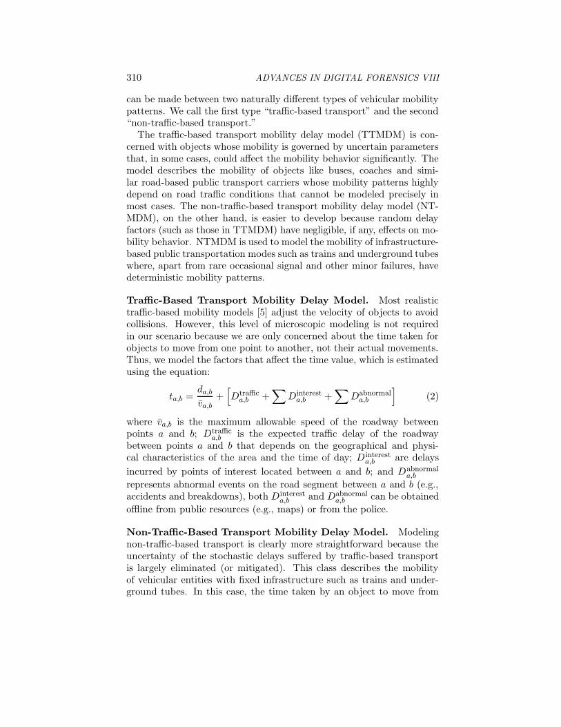
Traffic-Based Transport Mobility Delay Model. Most realistictraffic-based mobility models [5] adjust the velocity of objects to avoidcollisions. However, this level of microscopic modeling is not requiredin our scenario because we are only concerned about the time taken forobjects to move from one point to another, not their actual movements.Thus, we model the factors that affect the time value, which is estimatedusing the equation:

ta,b =da,b

v̄a,b+

!

Dtraffica,b +

"

Dinteresta,b +

"

Dabnormala,b

#

(2)

where v̄a,b is the maximum allowable speed of the roadway betweenpoints a and b; Dtraffic

a,b is the expected traffic delay of the roadwaybetween points a and b that depends on the geographical and physi-cal characteristics of the area and the time of day; D interest

a,b are delays

incurred by points of interest located between a and b; and Dabnormala,b

represents abnormal events on the road segment between a and b (e.g.,accidents and breakdowns), both Dinterest

a,b and Dabnormala,b can be obtained

offline from public resources (e.g., maps) or from the police.

Non-Traffic-Based Transport Mobility Delay Model. Modelingnon-traffic-based transport is clearly more straightforward because theuncertainty of the stochastic delays suffered by traffic-based transportis largely eliminated (or mitigated). This class describes the mobilityof vehicular entities with fixed infrastructure such as trains and under-ground tubes. In this case, the time taken by an object to move from


point a to point b can be computed using the classical distance equation:

ta,b =da,b

va,b+

!

Dabnormala,b

where va,b is the fixed speed of the object on its journey from a to bspanning a distance da,b (which can be obtained offline).

3.3 Multimodal Mobility Delay Model

Conventionally, when modeling the mobility of a particular object, itis implicitly assumed that the object’s behavior is consistent through-out the simulation. However, in our scenario, we cannot rule out thepossibility that the target could have used multiple different transporta-tion modes, each with different mobility characteristics. Thus far, wehave introduced three mobility delay models (PMDM, TTMDM andNTMDM). We now model the transition between them by constructinga multimodal mobility model (MMM) to assure a continuous flow of thetarget. Essentially, MMM only models the “transition behavior” be-tween two different models (or two different carriers of the same model)because, once the transition is completed, the relevant mobility model iscalled to simulate the mobility of the next part of the journey until an-other transition is required. A “homogenous” transition occurs betweentwo carriers of the same mobility model (e.g., changing a bus). On theother hand, a “heterogeneous” transition occurs between two carriers ofdifferent mobility models (e.g., changing from a bus to a train).

In a vehicular setting, we are interested in tracking the target who istransported by a carrier vehicle, not the vehicle itself; thus, the entitywho makes the transition must be modeled. Clearly, in PMDM, boththe entity and the carrier are a single component. When an entity shiftsfrom any model to PMDM, the transition is smooth and incurs no delay(i.e., an individual does not have to wait before commencing a “walk”behavior). For any other situation, however, transition modeling is re-quired to calculate the time an entity waits before shifting to the nextmodel (or carrier). The main idea is to observe the timetables of thecarriers at the transition location and calculate the transient wait time.

In a level-1 transition, the entity shifts from PMDM to TTMDMor NTMDM. In both cases, the entity most likely experiences a slighttransient delay due to the time interval between its arrival at locationx and when the next carrier belonging to the intended model departs.Therefore, as soon as the entity arrives at x, it checks the intendedcarrier’s timetable for the next departure time at its current locationbased on the current time and calculates the time difference. We will


discuss this process in detail when we describe a level-2 transition, whichgeneralizes a level-1 transition.

Recall that in our scene graph GM roadways are represented by edgesEGM and intersections by vertices VGM . A transition can only occur atan intersection, so let vi ∈ VGM be a transition vertex at which n carriersfrom either TTMDM or NTMDM stop. Let these carriers be denotedby R1, R2, . . . , Rn (this information is included in the label of vi; seeSection 2). The first step is to obtain the timetables of the n carriersTR1 , TR2 , . . . , T Rn and convert them into matrices MR1 ,MR2 , . . . ,MRn ,where the rows represent stops and the columns represent journeys.

Note that the dimensions of the matrices depend on the timetablesand may be different for different carriers. Next, we extract the rowscorresponding to vi from MR1 ,MR2 , . . . ,MRn and create a 3D matrixMvi by superposing the rows.

The dimensions of this new 3D matrix M vi are 1× L× n, such that:

L = max{w(MR1), w(MR2), . . . , w(MRn)}

where w(M) is the width (number of columns) of matrix M . In otherwords, L is the number of journeys made by the carrier Ri that makesthe highest number of journeys where i ∈ {1, 2, . . . , n}. Obviously, ifR1, R2, . . . , Rn do not all make the same number of journeys, M vi wouldcontain some undefined values. We assume access to a global clockthat returns the current time when the function cT ime() is invoked.After Mvi is created, c = cT ime() is used to build a 1 × n matrixM̂vi = [m1,1,m1,2, . . . ,m1,n] such that:

m1,j =

⎧

⎪

⎨

⎪

⎩

|c−m1,j,z| + ϵ if z ≥ c ≥ z + 1

ϵ if c = z or c = z + 1

∞ otherwise

where ϵ is a random delay representing the factors that may hold the car-riers (e.g., traffic) plus the wait time at each stop. The matrix M̂vi nowindicates how long an entity at the current location x has to wait to pick acarrier R1, R2, . . . , Rn passing by x (regardless of whether R1, R2, . . . , Rn

belong to the same or different models). In particular, the matrix listsall the carriers that stop at vi along with their delay times.

4. Trace Reconstruction

Classical missing data algorithms, such as EM [3] and data augmenta-tion [7], cannot be directly used in our scenario because the algorithmsprimarily make statistical inferences based on incomplete data, but do


not reconstruct traces. Additionally, it cannot be assumed that a suf-ficiently large number of available traces are available in order to usethese algorithms. Iterative sampling algorithms, such as Markov chainMonte Carlo (MCMC) [4], even when adapted for missing data, cannotbe used for the same reasons. Instead, we take a different algorithmicapproach to fill the “gaps” formed by the missing traces. We developan efficient reconstruction algorithm that, using mobility delay models,selects the route(s) that the target most likely has taken through a gapgiven the time it spent traversing the gap. In the worst case scenario,the algorithm eliminates several routes that the target could not possiblyhave taken, which may still constitute important evidence.

The reconstruction algorithm AR first considers each gap individu-ally and reconstructs the gap. The reconstructed gaps are connected toobtain the full trace of a target s.

Abstractly, AR has two fundamental building blocks: (i) a multi-graph traversing algorithm called weight-bound-search (WBS); and (ii)various mobility models. After AR is executed, the reconstruction al-gorithm proceeds by running WBS over a gap. The WBS algorithm,in turn, repeatedly calls the mobility models (possibly via AR) and re-turns a route (or routes) that connect the gap. The AP algorithm thenreconstructs the other gaps in a similar fashion.

The WBS algorithm employs a branch-and-bound approach to opti-mize the reconstruction process, and uses a “crawler” to traverse gapsand find plausible routes. For a gap Gp : vm → vn between vertices vm

and vn where m,n ∈ {1, 2, . . . , |VGM |}, a crawler CGp is generated atvm and broadcasted toward vn. The crawler CGp maintains two datastructures: (i) a LIFO list of vertices and edges traversed χCGp ; and(ii) a delay variable τCGp . The variable χCGp is dynamically updatedwhenever CGp traverses a vertex or edge to keep track of all the verticesand edges that the crawler CGp has visited. The delay variable τCGp ,which is initially set to zero, is also dynamically updated whenever CGp

traverses an edge or an S-vertex (but not a U -vertex as described below).When CGp is first initiated at vm, it checks the vm label ℓm = {Ry

x, . . . ,Rl

k}, which contains information about the routes of which vm is a part

and locates its ℓ̂m next-hop neighboring vertices using the equation:

ℓ̂m =

!

|ℓm| if vm ̸∈ ←−ρ G

|ℓm|− k if vm ∈ ←−ρ G

where k is the number of times vm appears in ←−ρ G (number of routes inwhich vm is a tail-end vertex; these routes terminate at vm and thus donot have a next-hop).


Since we are considering a multi-graph, it is possible that some ofthe routes pass by the same next-hop neighbor (creating parallel edgesbetween two vertices), so the ℓ̂m list may contain repeated vertices. Ifthis is the case, each outgoing edge (even if all the edges are parallel)must be considered separately because the edge may have a differentweight depending on the route to which it belongs. Thus, after all thenext-hop neighbors are found, CGp selects one of them, say vu, finds theedges (routes) between vm and vu, i.e., {ei|ei : vm → vu}, and selectsone ei.

After an ei is selected, CGp tags it as “visited,” updates χCGp andproceeds to traverse it. It is important that CGp tags every traversededge as “visited” so that the edge is not revisited, potentially resultingin an infinite loop. Furthermore, if CGp arrives at a vertex vk and findsthat there is only one unvisited edge ei, it tags ei as “visited,” traversesit and then tags vk as “exhausted” so that vk is skipped if it happensto be a neighbor of some vertex that CGp traverses in the future. Basedon the type of the edges connecting vm with its next-hop neighboringvertices, CGp calls the appropriate mobility model (PMDM, TTMDMor NTMDM) to calculate the delay of the edge. Next, it updates τCGp

using the equation:

τCGp = τCGp + tvx,vy

where tvx,vy is the delay returned for the edge ei : vx → vy by the relevantmobility model (this applies to R- and W -edges). Similarly, when CGp

reaches an S-vertex vy, it again updates τCGp , but this time by callingMMM such that:

τCGp = τCGp + tvy

where tvy is the delay assigned to vy by MMM. However, since there isno transition between mobility models in U -vertices, MMM is not calledwhen a U -vertex is reached.

The crawler traverses the various routes by repeatedly backing-upwhenever it finds a plausible or implausible route. The back-up proce-dure proceeds as follows: when the crawler finds an (im)plausible route,it checks χCGp and traverses backward through the edge in χCGp [1] to-ward the vertex χCGp [2] where χ[n] is the nth element of the list χ. Next,it deletes the two elements from χCGp and repeats the entire traversalprocess, but this time it does not traverse the edge it just came frombecause it is now tagged as “visited” (or generally any edge tagged as“visited”).

The crawler CGp backs-up if: (i) τCGp + ϵ > tvn,vm ; or (ii) traverses avertex/edge that already exists in its χCGp ; or (iii) vn (other end of the


gap) is reached where ϵ is a random value; or (iv) reaches a vertex vj

such that vj is a tail-end vertex in all its routes (i.e., vj is childless).In (i), the crawler backs-up when τCGp reaches a value greater than

tvn,vm (time difference between when the target was observed at vm andlater at vn – corresponding to the two ends of a gap Gp), and ϵ is asmall constant. This means that the target would take much longerthan tvm,vn if it had traversed that route. In (ii), only loop-free routesare accepted because these are what a rational target would opt to take(they also prevent infinite loops); so, if CGp reaches a vertex vi such thatvi ∈ χCGp , then it backs-up. In (iii), when CGp reaches vn, it checksτCGp . If τCGp + ϵ ≤ tvm,vn − ϵ, it backs-up (in other words, if a crawlerreturns a time much shorter than tvm,vn , it is probably not the routethat the target has taken). Otherwise, if tvm,vn − ϵ ≤ τCGp ≤ tvm,vn + ϵ,it backs-up, returns the route in χCGp as a possible route the target mayhave taken and returns the corresponding τCGp . Finally, in (iv) CGp alsobacks-up when it reaches a childless vertex vj; additionally, it tags vj as“exhausted.”

The WBS algorithm terminates when its crawler terminates. Thisoccurs when the crawler reaches a vertex in which all neighboring (next-hop) vertices are tagged as “exhausted,” meaning that they have alreadybeen traversed extensively (i.e., all their outgoing edges are tagged as“visited”).

Proposition 2. Given a finite search graph, the WBS algorithm even-tually terminates with or without returning valid routes.

Proof. Since the WBS is a weight-based algorithm, it is guaranteed tostop traversing a particular route Ri when its weight counter τCGp ex-pires (i.e., τCGp ≥ tvm,vn + ϵ where tvm,vn is the delay through gapGp : vm → vn and ϵ is a small constant). Thus, the only way forthe algorithm to run indefinitely is when it gets into an infinite loopand traverses the same route over and over again. However, a route Ri

cannot be traversed more than once because the algorithm tags everyvisited edge and does not traverse any tagged edge. Thus, the algorithmterminates as long as the graph has a finite number of edges.

The WBS algorithm also terminates when processing an infinitelydeep graph because it traverses the graph down to the point when itsweight counter τCGp expires. However, the WBS algorithm may fail toterminate when processing an infinitely wide graph if none of the childrenof the current level has a weight higher than τCGp . This, nevertheless,contributes to the completeness of the WBS algorithm.


Proposition 3. Given a finite search graph, the WBS algorithm is com-plete. If multiple solutions exist, the algorithm returns all the solutions.

Proof. For a gap Gp : vm → vn, a valid solution means that there is aroute Ri : vm → vn with a weight τ such that tvm,vn− ϵ ≤ τ ≤ tvm,vn + ϵ.The crawler CGp traverses all valid and invalid routes and terminateswhen there are no more edges to traverse. Therefore, if such a solutionroute Ri exists, the crawler CGp will find the route.

If multiple routes are returned after the crawler terminates, then thealgorithm selects the “best-fit” route such that:

|χC

Gpf

| = min{|χC

Gp1

|, |χC

Gp2

|, . . . , |χC

Gpn

|}.

The route with less hops is selected because a rational target wouldprobably choose a route that does not have many stops. Additionally,by observing the labels of the edges and vertices of the returned routes, apreferred route can be selected that minimizes the number of transitionsbetween different mobility models and/or carriers with the same model.

5. Conclusions

The multi-modal trace reconstruction algorithm described in this pa-per engages mobility models tailored for forensic analysis to construct acomplete trace of a target who may use multiple modes of transporta-tion. Gaps of missing data between the points where the target wasobserved are filled by considering all possible routes through the gapsinvolving pedestrian routes, public routes and a combination of both.Theoretical analysis of the reconstruction algorithm demonstrates thatit is both complete and optimal. Certain details have been omittedfor reasons of space. Interested readers may contact the authors for acomplete description of the algorithm and the accompanying theoreticalanalysis.

References

[1] S. Al-Kuwari and S. Wolthusen, Probabilistic vehicular trace re-construction based on RF-visual data fusion, Proceedings of theEleventh IFIP TC 6/TC 11 International Conference on Commu-nications and Multimedia Security, pp. 16–27, 2010.

[2] S. Al-Kuwari and S. Wolthusen, Fuzzy trace validation: Toward anoffline forensic tracking framework, Proceedings of the Sixth IEEEInternational Workshop on Systematic Approaches to Digital Foren-sic Engineering, 2011.


[3] A. Dempster, N. Laird and D. Rubin, Maximum likelihood fromincomplete data via the EM algorithm, Journal of the Royal Statis-tical Society, Series B (Methodological), vol. 39(1), pp. 1–38, 1977.

[4] W. Gilks, S. Richardson and D. Spiegelhalter (Eds.), Markov ChainMonte Carlo in Practice, Chapman and Hall/CRC Press, Boca Ra-ton, Florida, 1996.

[5] J. Harri, F. Filali and C. Bonnet, Mobility models for vehicularad hoc networks: A survey and taxonomy, IEEE CommunicationsSurveys and Tutorials, vol. 11(4), pp. 19–41, 2009.

[6] D. Helbing and P. Molnar, Social force model for pedestrian dy-namics, Physical Review E, vol. 51(5), pp. 4282–4286, 1995.

[7] M. Tanner and W. Wong, The calculation of posterior distributionsby data augmentation, Journal of the American Statistical Associ-ation, vol. 82(398), pp. 528–540, 1987.

Forensic Tracking and Mobility Prediction in Vehicular...

Documents

Transcript of Forensic Tracking and Mobility Prediction in Vehicular...