FINAL REPORT FATIGUE RELIABILITY OF STEEL … fracture failure subsequent to fatigue cracking is the...

$: FINAL REPORT FATIGUE RELIABILITY OF STEEL … fracture failure subsequent to fatigue cracking is the most common cause of steel bridge component failure and occurs in bridges mainly$
FINAL REPORT

FATIGUE RELIABILITY OF STEEL HIGHWAY BRIDGE DETAILS

Peter J. Massarelli, Ph.D.

Faculty Research Associate

Thomas T. Baber, Ph.D. Faculty Research Scientist

Virginia Transportation Research Council

(A Cooperative Organization Sponsored Jointly by the Virginia Department of Transportation and

the University of Virginia)

In Cooperation with the U.S. Department of Transportation Federal Highway Administration

Charlottesville, Virginia

August 2001 VTRC 02-R4

ii

DISCLAIMER

The contents of this report reflect the views of the authors, who are responsible for the facts and the accuracy of the data presented herein. The contents do not necessarily reflect the official views or policies of the Virginia Department of Transportation, the Commonwealth Transportation Board, or the Federal Highway Administration. This report does not constitute a standard, specification, or regulation.

Copyright 2001 by the Commonwealth of Virginia.

iii

ABSTRACT

The expected life of a steel highway bridge subjected to random, variable-amplitude traffic cycles is highly dependent on damage accumulation caused by various fatigue mechanisms. This study addressed some of the issues associated with developing probabilistic reliability models for steel bridge structures under vehicular traffic loadings. Specifically, methods for incorporating inspection data (e.g., the presence and size of cracks) into classical and fracture mechanics–based fatigue models to predict fracture-critical element damage accumulation were analyzed.

The block loading method introduced here assigns a damage state to the cracked detail after each vehicle passage. This method is limited to loading blocks where the plastic zone at the crack tip developed by the pseudo-static response of the bridge must be larger than the crack growth caused by the subsequent dynamic cycles for each vehicle passage. It must also be assumed that the crack length is fixed during a loading block. This method accounts for closure effects by predicting the occurrence of damage only when the crack is opened. When a bridge inspection reveals fatigue cracks, field data in the form of strain measurements can be collected in the vicinity of the fracture detail to identify the characteristic stress block and the fluctuations in the curve attributes attributable to randomness of the traffic loading. Then, the data can be analyzed to identify the statistical properties of the attribute parameters, which include the magnitude of the pseudo-static response, the number of dynamic cycles in each block, and the duration of the vehicle passage. With this information, the distribution of stress blocks can be estimated, and the block loading method can be employed to calculate the fatigue lifetime of each critical detail.

FINAL REPORT

FATIGUE RELIABILITY OF STEEL HIGHWAY BRIDGE DETAILS

Peter J. Massarelli, Ph.D. Faculty Research Associate

Thomas T. Baber, Ph.D.

Faculty Research Scientist

INTRODUCTION

Fatigue and fracture behavior are important considerations in determining the condition of metal structures subjected to cyclic loads. Specifically, the expected life of a steel highway bridge subjected to random, variable-amplitude traffic cycles is highly dependent upon damage accumulation caused by various fatigue mechanisms. The analysis of structural fatigue damage is generally divided into two concerns: resistance and load. Resistance refers to the load-carrying capabilities of the structure, and load encompasses the external forces applied to the structure. Structural failure is seldom attributed to load considerations; the occurrence of stresses exceeding those predicted by the designer is rare. Brittle fracture failure subsequent to fatigue cracking is the most common cause of steel bridge component failure and occurs in bridges mainly because specific details have a lower fatigue resistance than the designers originally thought (Fisher, 1984).

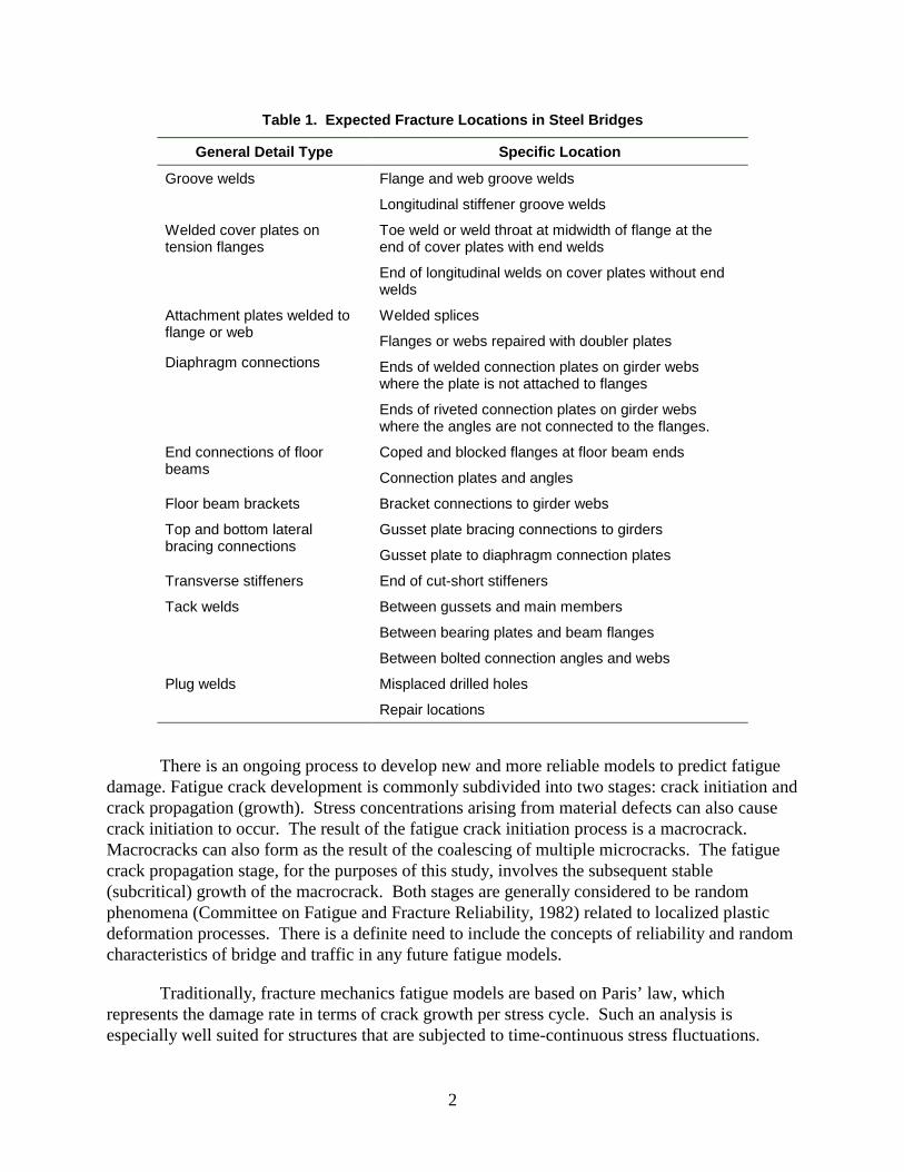
Fisher and Yuceoglu (1981) compiled qualitative data concerning the cracking of 142 bridges in the United States and Canada. They identified out-of-plane distortion and large initial defects as the two most common specific causes of fatigue crack development. Barsom and Rolfe (1987) attributed component distortion to the residual stresses that sometimes arise after welding materials have cooled, and they reported that welding may also be responsible for a number of the initial defects such as gas pockets, undercuts and cracks. A number of specific details in steel bridges have been identified as being especially susceptible to cracking. Xanthakos (1994) compiled a list of expected fracture locations that is summarized in Table 1.

Stress-life fatigue analysis is currently based on the so-called S-N diagrams that relate N (loading cycles to failure) and the amplitude or range of the applied cyclic stress S. However, the empirical nature of stress-life methods imposes severe limitations on the usefulness of S-N data. The S-N method does not account for the true stress-strain response of the material; local plasticity effects are ignored and all strains are considered to be elastic; and any unusual detail geometry would preclude the application of preexisting data. Despite the limitations of classical fatigue methods, the S-N approach to fatigue analysis is the basis for the current American Association of State Highway and Transportation Officials (AASHTO) design specifications.

2

There is an ongoing process to develop new and more reliable models to predict fatigue damage. Fatigue crack development is commonly subdivided into two stages: crack initiation and crack propagation (growth). Stress concentrations arising from material defects can also cause crack initiation to occur. The result of the fatigue crack initiation process is a macrocrack. Macrocracks can also form as the result of the coalescing of multiple microcracks. The fatigue crack propagation stage, for the purposes of this study, involves the subsequent stable (subcritical) growth of the macrocrack. Both stages are generally considered to be random phenomena (Committee on Fatigue and Fracture Reliability, 1982) related to localized plastic deformation processes. There is a definite need to include the concepts of reliability and random characteristics of bridge and traffic in any future fatigue models.

Traditionally, fracture mechanics fatigue models are based on Paris’ law, which represents the damage rate in terms of crack growth per stress cycle. Such an analysis is especially well suited for structures that are subjected to time-continuous stress fluctuations.

Table 1. Expected Fracture Locations in Steel Bridges

General Detail Type Specific Location

Groove welds Flange and web groove welds

Longitudinal stiffener groove welds

Welded cover plates on tension flanges

Toe weld or weld throat at midwidth of flange at the end of cover plates with end welds

End of longitudinal welds on cover plates without end welds

Attachment plates welded to flange or web

Welded splices

Flanges or webs repaired with doubler plates Diaphragm connections Ends of welded connection plates on girder webs

where the plate is not attached to flanges

Ends of riveted connection plates on girder webs where the angles are not connected to the flanges.

End connections of floor beams

Coped and blocked flanges at floor beam ends

Connection plates and angles

Floor beam brackets Bracket connections to girder webs

Top and bottom lateral bracing connections

Gusset plate bracing connections to girders

Gusset plate to diaphragm connection plates

Transverse stiffeners End of cut-short stiffeners

Tack welds Between gussets and main members

Between bearing plates and beam flanges

Between bolted connection angles and webs

Plug welds Misplaced drilled holes

Repair locations

3

However, the loading on bridge structures caused by vehicular passages is more episodic in nature. Through the field testing of numerous bridges, it has been observed that the stress block induced by the passage of a single vehicle has common attributes for a particular bridge that are dependent upon its construction and road surface. Random vehicle factors (such as weight, speed, and suspension properties) determine its precise shape. Typically, each stress block is characterized by a dominant pseudo-static portion superimposed with higher frequency dynamic fluctuations and followed by a transient die-out. Accordingly, this study suggests a proposed model that treats a vehicle passage as a randomly arriving discrete block of stress cycles and calculates crack growth per loading block, as opposed to crack growth per stress cycle. Further, the model accounts for crack closure effects by predicting the occurrence of damage only when the crack is opened.

PURPOSE AND SCOPE

The objective of this study was to develop a simplified method of predicting the fatigue reliability of steel bridge details with preexisting cracks. The expected life of a steel highway bridge subjected to random, variable-amplitude traffic cycles is highly dependent upon damage accumulation caused by various fatigue mechanisms. The proposed probabilistic model mainly addresses randomness associated with the stress spectra imposed upon the cracked detail by vehicular passages. Specifically, a method of incorporating inspection data (e.g., the presence and size of cracks) into a fracture mechanics–based fatigue model to predict detail reliability is proposed. The proposed model treats a vehicle passage as a randomly arriving discrete block of stress cycles and calculates crack growth per loading block as opposed to crack growth per stress cycle.

BACKGROUND

Linear Elastic Fracture Mechanics (LEFM) and Fatigue

When a defect is present in a material, a fracture mechanics approach provides the most insightful analysis of fatigue crack propagation. In 1957, Irwin formulated the following fundamental equation of fracture mechanics that describes the stress at a point (r,θ) near the tip of a crack:

( )σπ

θij ij

Kr

f=2

[1]

where K is the stress intensity factor and fij(θ) are known functions of θ, r is the radial distance from the crack tip, and θ is the angle relative to a reference coordinate.

The stress intensity factor has a general form

( )K f g a= σ π [2]

4

where σ is the stress applied away from the crack, called the far-field stress, a is the crack length, and f(g) is a correction factor that depends on specimen and crack geometry (Bannantine et al., 1990). Fracture mechanics is rooted in the supposition that conditions at the tip of a crack can be uniquely defined by the stress intensity factor and that unstable crack growth will occur when the stress intensity factor at the crack tip exceeds the critical stress intensity factor, Kc, which is a material property.

In order to employ LEFM-based fatigue analyses, the presence and size of a crack must be determined. Xanthakos (1994) compiled a list of expected fracture locations, summarized in Table 1, and Fisher (1984) did extensive work estimating the stress intensity factors for these types of fatigue critical details.

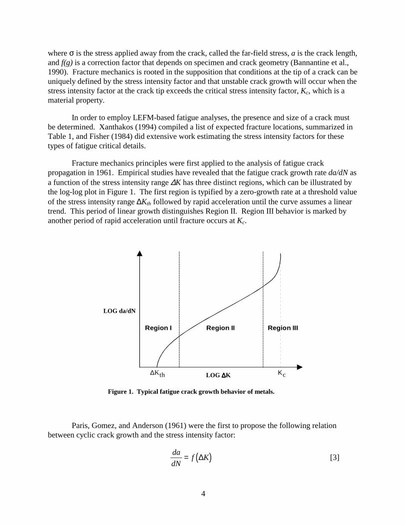
Fracture mechanics principles were first applied to the analysis of fatigue crack propagation in 1961. Empirical studies have revealed that the fatigue crack growth rate da/dN as a function of the stress intensity range ∆K has three distinct regions, which can be illustrated by the log-log plot in Figure 1. The first region is typified by a zero-growth rate at a threshold value of the stress intensity range ∆Kth followed by rapid acceleration until the curve assumes a linear trend. This period of linear growth distinguishes Region II. Region III behavior is marked by another period of rapid acceleration until fracture occurs at Kc.

Region IIRegion I Region III

LOG ∆∆∆∆K

LOG da/dN

∆Kth Κc

Figure 1. Typical fatigue crack growth behavior of metals.

Paris, Gomez, and Anderson (1961) were the first to propose the following relation between cyclic crack growth and the stress intensity factor:

( )dadN

f K= ∆ [3]

5

where ∆K equals Kmax – Kmin. In 1963, Paris and Erdogan elaborated on Equation 3 and presented the formulation that is widely known as the Paris law or the Paris-Erdogan equation:

( )dadN

C K m= ∆ . [4]

C and m are material constants that were subsequently tabulated for a wide range of metals. The Paris law describes Region II crack growth.

When visual or nondestructive inspection (NDI) techniques reveal flaws or macrocracks in structural components, the fatigue life of the component is governed by the rate of subcritical crack propagation. Barsom and Rolfe (1987) presented data obtained from constant-amplitude cyclic loading tests for A514 and A533, Grade B steels. These data, which are available for many laboratory environments, are used to determine C and m in Equation 4 to establish the crack growth rate of these materials.

The fatigue life of actual structural components subjected to variable-amplitude loading (such as random traffic loads) can differ greatly from components subjected to constant-amplitude stress cycles in the laboratory. For classical fatigue analysis, the Palmgren-Miner rule (or simply Miner’s rule) of linear damage accumulation is frequently used to account for variable-amplitude stresses. A cycle-counting algorithm is employed to quantify and differentiate cycles by stress range, and then the damage of each range is superposed to approximate the total damage. However, this method ignores highly important sequence effects, such as crack retardation after tensile overloads sufficiently greater than previous and subsequent cycles.

Despite these problems, some success has been achieved in predicting the fatigue life of steel components subjected to random loads. Barsom (1973) developed what is known as the root mean square (RMS) method of relating variable-amplitude stress histories to constant-amplitude, fracture mechanics-based fatigue data. This is performed by calculating an effective change in stress intensity, ∆Krms, based on a statistical analysis of the load history.

Experimental analysis suggests that crack growth rates predicted by this method are compatible with the growth rate of cracks under different loading sequences. Barsom and Novak (1977) employed the RMS method to study crack propagation in a variety of bridge steels under corrosive and non-corrosive fatigue environments. They concluded that this modification of Paris’ law was effective in predicting crack growth behavior for A36, A588, and A514 structural steels. However, the random loading spectra used in their experiments were simulated.

It has been observed that crack growth predictions are also a function of crack closure. Elber (1971) suggested that crack closure slowed the fatigue crack growth rate by effectively decreasing the stress intensity range. Crack closure occurs when crack faces remain together for stress intensity levels greater than Kmin. Kim and Song (1994) performed numerous fatigue crack growth tests under random loading to investigate the behavior of crack closure in detail. As a

6

result of this study, they proposed a simple model that includes closure effects for predicting fatigue crack growth under block spectrum loading. The model proposed in the present study is based on the results of their experiments.

Kim and Song (1994) concluded that the crack opening load is mainly governed by the largest load cycle in a random loading block because their tests indicated that Kop is nearly identical for both narrow and wide band spectra. Another relevant conclusion was that the opening stress intensity of a single random loading block is linearly proportional to the stress intensity factor of the maximum loading cycle in that block. Thus,

( ) ( )K Kop i i∝ max [5]

for a random stress block, i.

Structural Reliability Techniques

Reliability is the probability measure of whether a system will perform a specified function under given conditions for a prescribed amount of time. It is the complementary probability of the cumulative distribution frequency of system failure. Bridge component failure is defined as violating a predefined limit state. Limit states are of three types (Melchers, 1987): ultimate (e.g., collapse and fracture), damage (e.g., excessive cracking), and serviceability (e.g., large deflection and exceeding a code requirement). Along with defining a limit state, a first step of reliability analysis should be identifying uncertainties. Each uncertainty is considered a basic random variable, and a probability density function must be assigned to each of these variables.

Reliability models that rely upon deterministic structural analysis and empirically based fatigue models have proven inadequate. Probabilistic reliability models are better suited for predicting structure lives because of the randomness inherent in both load and resistance considerations. It has come to be accepted that fatigue crack initiation and growth are functions of random phenomena. The empirical models frequently used to analyze fatigue do not suitably account for the effects of out-of-plane loading and large defects that Fisher and Yuceoglu (1981) identified as the major causes of structural failure.

A model based on the Markov decision process for evaluating bridge reliability was developed by Tao, Ellis, and Corotis (1995), which accounts for corrosion-driven structural deterioration and human intervention (maintenance and repair). However, their model was designed to predict overall bridge reliability and does not address fatigue concerns explicitly. The model developed in the present study focuses exclusively on fatigue reliability.

LEFM Approach to Fatigue Crack Growth

In recent years, much research has been conducted to identify reliability solutions for the stochastic fatigue crack growth problem. Tang and Spencer (1989) used a cubic crack growth law (in lieu of Paris’ law) to model experimental data stochastically. The crack growth equation

7

was multiplied by a random variable using normal, lognormal, and Weibull probability distributions. The mean and variance of a random time to reach a critical crack size were comparable for each of the distributions and matched the data well. Itagaki, Ishizuka, and Yan (1993) formulated a crack growth reliability prediction by modeling the material parameters of Paris law, C and m, as random variables. From experimental analyses, they concluded that m can be approximately represented by a normal variate and (1/C) with a three-parameter Weibull distribution.

Specific applications to bridge structures are rare, but an alternative to the AASHTO method (AASHTO, 1989) was presented by Zhao, Haldar, and Breen (1994a,b) that uses a fracture mechanics approach. The limit state for this method is

α αc N− ≤ 0 [6]

where αN is the in-service crack size after N stress cycles and αc is the critical crack size. The critical crack size can be either the crack size where unstable crack growth begins to occur or the crack size where a serviceability requirement is exceeded. The uncertainties involved in this analysis are the initial crack size, the crack initiation period, the geometry function for each specific detail, and the material properties C and m that appear in the Paris-Erdogan equation. The advantage of this method is that inspection data can be incorporated into the reliability analysis to update fatigue life predictions throughout the service life of the bridge.

Characteristic Stress Block identification It has been observed that the stress block induced by the passage of a single vehicle has a

characteristic shape for a particular bridge that is dependent upon its construction and road surface. Random vehicle factors, such as weight and axle distribution, speed, and suspension characteristics, determine its magnitude and cyclic frequency. Typically, each stress block is characterized by a dominant pseudo-static portion, superimposed with higher frequency dynamic fluctuations, and followed by a transient die-out. The concept of a stress or loading block is an important aspect of this study. Because the induced stresses of each truck passage have similar characteristics, the proposed methodology attempts to calculate the fatigue damage per loading block, as opposed to per stress cycle. Doing so offers many advantages. The number of random variables is greatly reduced, the data collection requirements are far less stringent, and crack closure considerations can be readily included into the fatigue model.

Bannantine et al. (1990) presented one method of predicting the fatigue life of a cracked specimen where crack growth per loading block is calculated. This method is based on a loading block model proposed by Brussat (1974) that was originally designed for aircraft structures. An advantage of this model is the computational efficiency it offers when compared with stress cycle summation techniques. This model also lends itself well to the vehicular loading of bridges because of the episodic nature of stress records imposed by truck passages. It is limited to loading blocks where the crack growth is not large enough to extend past the plastic zone formed by the largest load cycle per block. It is also assumed that the actual loading history can be modeled by a repeating block of loading and that crack length is fixed during a loading block.

8

This method accounts for closure effects by predicting the occurrence of damage only when the crack is opened. The effective change in stress intensity factor ∆Keff is determined by first choosing a crack opening stress level, σop. It is assumed that the opening stress remains constant for every cycle in the block. This is consistent with the assumption of Sunder (1992) and the experimental analysis of Kim and Song (1994). The effective stress for the ith cycle in the block is then related to the opening stress by

( ) ( )∆σ σ σeff i i op= −max [7]

Thus, if a block contains a periodic overload, the opening stress corresponding to the overload will dominate and no crack extension will result from subsequent stress cycles in the block that have a maximum value below σop.

Data Analysis

Because the stress pattern obtained from traffic data does not have a constant amplitude and uniform frequency, a systematic approach to counting stress cycles is needed. Various cycle-counting algorithms have been developed for reducing complex histories into a finite number of variable amplitude cycles. Among the earliest of these are the level-crossing counting, peak counting, and simple range counting techniques (Bannantine et al., 1990).

Level-crossing counting involves dividing the stress axis into an arbitrary number of equal increments. A reference stress is initially chosen, and each time a positively sloped portion of the stress record crosses an increment above the reference stress, a count is recorded for that particular increment value. Likewise, each time a negatively sloped portion of the stress history crosses an increment value below the reference stress, a count is recorded. Then, the counts are combined to form full cycles. Frequently, this is done by combining the counts to form the largest possible cycle, and the remaining counts are combined to form the next largest possible cycle, etc. When all counts have been assigned to a cycle, the process is completed.

Peak counting also involves dividing the stress axis into increments and choosing a reference stress. All local maxima above the reference stress and all local minima below the reference stress are recorded. Then, these counts are combined by sequentially grouping the greatest maxima with the least minima to form complete cycles.

Simple range counting involves recording the range between successive stress reversals and counting each range as one half-cycle.

There are certain limitations to these cycle-counting techniques. Mainly, each method disregards the actual sequence of applied stress cycles. Consequently, in the late 1960s, a new type of cycle counting algorithm was developed that attempted to identify closed hysteresis loops in the stress-strain response of a material under cyclic-loading. The term rainflow counting has been applied to the general family of such algorithms. Hoadley, Frank, and Yura (1983)

9

conducted an extensive review of various cycle counting schemes and concluded that rainflow counting methods are the most suitable for the study of highway bridges under traffic loading.

METHODOLOGY

Description of Proposed Model

The proposed model attempts to develop a reliability prediction for a fatigue-critical bridge detail when a measurable crack has been detected. This model bases its reliability prediction upon the size of the crack at inspection time and probabilistic aspects of future loading. When a bridge inspection has revealed that a specific detail has a crack of size a0, the following steps must be taken:

1. Determine an equation for the stress intensity factor.

2. Estimate the stress at the detail location attributable to dead load from strength of materials techniques or a finite-element analysis, if applicable. It is assumed that a method of measuring in- situ non-live load bridge stresses will not be available.

3. Take strain data in the vicinity of the crack for a representative sample of truck passages. It is customary to assume that fatigue damage caused by automobiles and other smaller vehicles is negligible compared to the damage caused by trucks. This is well established in the AASHTO design guidelines (AASHTO, 1983) and is the rationale for neglecting stress cycles below 1 ksi.

4. Break up the strain (stress) data into equal time interval records reflecting individual truck passages. Then, process each record through an appropriate cycle-counting algorithm.

5. Calculate the probability of damage in terms of crack extension caused by a single loading block (truck passage).

6. After the probabilistic features of the stress loading block have been established, determine the reliability calculation for the detail in question.

The general form of the stress intensity factor K was given in Equation 2. Calculating the effective change in stress intensity factor for each loading cycle in the block is accomplished with the use of the traditional fracture mechanics relationship

( ) ( ) ( )∆ ∆K a f geff i eff i b b= σ π [8]

where ab is the crack length and f(gb) is a function of the geometry of the fatigue detail and of the crack during the bth loading block.

10

The following form of Paris’ law is then used to calculate the change in crack length per loading cycle in each block:

( )[ ]∆ ∆a C Ki eff i

m= , [9]

where m is the material crack growth exponent and C is the material crack growth coefficient. As mentioned previously, this is also the equation employed by Kim and Song (1994) in their prediction of fatigue crack growth under variable amplitude loading. It is important to note here that Paris’ law was developed to describe the Region II crack growth behavior shown in Figure 1. By employing this crack growth rate equation, the model ignores the presence of a threshold stress intensity range. Thus, Paris regime behavior is assumed to extend to stress range levels below those corresponding to ∆Kth. Consequently, the proposed model may predict overly conservative fatigue lifetimes by assuming that a crack may propagate at ∆K ranges below ∆Kth. The total change in crack length per block b can be calculated by summing the changes per cycle such that

( )[ ] ( )∆∆

∆ ∆ab

a C a f gb

ii

n

bb b

m

effi

n

i

m�

��

��=�

��

�

�� =

= =� �

1 1π σ , [10]

where n is the total number of cycles in the bth loading block. Because of the assumption that the block is repeating,

( )∆σ effi

n

i

m

=�

1

[11]

remains constant for every block.

Damage Stress Function

The proposed probabilistic model modifies the block loading method described previously by assuming that the stress block is not repeated. Instead of assuming that one block of stress cycles is repeatedly applied to the cracked detail, the blocks in the proposed model are treated stochastically. The blocks, although similar in shape, will possess varying amplitudes consistent with the variability of vehicular parameters, including weight and speed. Thus, the concept of a damage stress function is defined.

It is assumed that the pseudo-static overload cycle establishes a crack opening stress, ∆σop, which must be surpassed by subsequent loading cycles in the block for damage to occur. The damage stress function is then given as

( )[ ] ( ) ( )( )h B i op

m

i

n

ω σ σω ω= −=�

1 [12]

11

where σi are the cycles following the overload that exceed σop, n is the total number of cycles in each loading block that meet this criterion, and ω is the particular outcome in the space of all vehicles for which the block damage is expressed.

Data Collection and Reduction

After a crack is identified, a field test must be conducted to obtain the strain response in the vicinity of the crack to a statistically significant number of truck passages. The strain (stress) data can then be broken up into records of equal time intervals to reflect individual truck passages. When recording the strain data in the field, the strain or weigh-in-motion (WIM) gages must be oriented correctly and the strain records must be sampled at a sufficiently high rate to ensure that critical features of the stress block are present.

Typical stress records for two random truck passages are given in Figure 2. These data were recorded with a WIM gage attached to the bottom flange of an interior girder of the I-64 bridge over Route 22 in Shadwell, Virginia. Elastic behavior was assumed, and the induced stress records were found by multiplying the recorded strain values by Young’s modulus of the detail material. (Hundreds of similar stress records were also recorded; however, for the sake of brevity, certain aspects of the proposed methodology will be demonstrated using these two loading blocks, which will henceforth be called Records 18 and 19, respectively.) Note that the stress record has a zero-baseline. The stress attributable to dead load effects is superimposed later in the analysis.

The next step is to calculate the probability of damage in terms of crack extension caused by a single loading block (truck passage). The suggested block loading method is an approximate model that attempts to develop a prediction of damage caused by a single vehicle passage as a separable function of crack geometry and stress loading. When the probabilistic

Time (sec)

Stre

ss (M

Pa)

I-64 Bridge Over Rte. 22, Record 18Mid-Span of Interior Girder, Bottom Flange

0 0.6 1.2 1.8 2.4 3 3.6 4.2 4.8 5.4 6-3

-1.5

0

1.5

3

4.5

6

7.5

9

Time (sec)

Stre

ss (M

Pa)


0 0.6 1.2 1.8 2.4 3 3.6 4.2 4.8 5.4 6-3

-1.5

0

1.5

3

4.5

6

7.5

9

Figure 2. Stress records for two random truck passages.

12

features of the stress loading block are established, the reliability calculation for the detail in question can be calculated.

Rainflow Cycle Counting

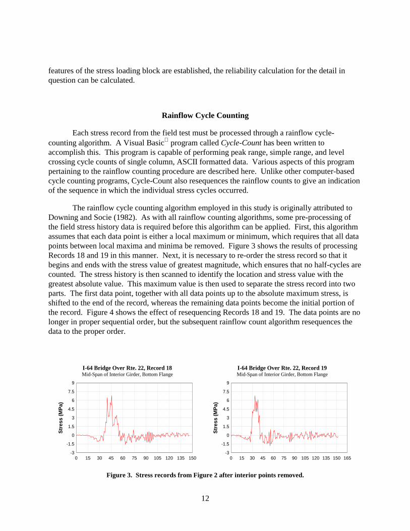
Each stress record from the field test must be processed through a rainflow cycle-counting algorithm. A Visual Basic program called Cycle-Count has been written to accomplish this. This program is capable of performing peak range, simple range, and level crossing cycle counts of single column, ASCII formatted data. Various aspects of this program pertaining to the rainflow counting procedure are described here. Unlike other computer-based cycle counting programs, Cycle-Count also resequences the rainflow counts to give an indication of the sequence in which the individual stress cycles occurred.

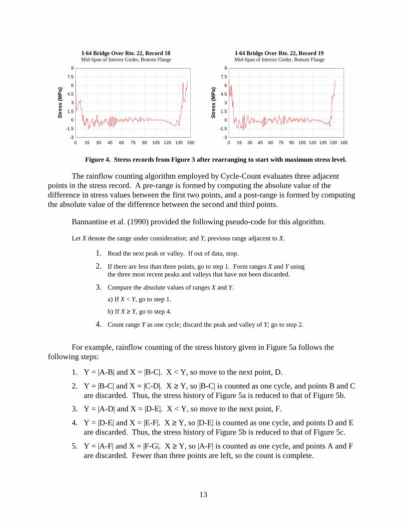
The rainflow cycle counting algorithm employed in this study is originally attributed to Downing and Socie (1982). As with all rainflow counting algorithms, some pre-processing of the field stress history data is required before this algorithm can be applied. First, this algorithm assumes that each data point is either a local maximum or minimum, which requires that all data points between local maxima and minima be removed. Figure 3 shows the results of processing Records 18 and 19 in this manner. Next, it is necessary to re-order the stress record so that it begins and ends with the stress value of greatest magnitude, which ensures that no half-cycles are counted. The stress history is then scanned to identify the location and stress value with the greatest absolute value. This maximum value is then used to separate the stress record into two parts. The first data point, together with all data points up to the absolute maximum stress, is shifted to the end of the record, whereas the remaining data points become the initial portion of the record. Figure 4 shows the effect of resequencing Records 18 and 19. The data points are no longer in proper sequential order, but the subsequent rainflow count algorithm resequences the data to the proper order.

Stre

ss (M

Pa)


0 15 30 45 60 75 90 105 120 135 150-3

-1.5

0

1.5

3

4.5

6

7.5

9

Stre

ss (M

Pa)


0 15 30 45 60 75 90 105 120 135 150 165-3

-1.5

0

1.5

3

4.5

6

7.5

9

Figure 3. Stress records from Figure 2 after interior points removed.

13

Stre

ss (M

Pa)


0 15 30 45 60 75 90 105 120 135 150-3

-1.5

0

1.5

3

4.5

6

7.5

9

Stre

ss (M

Pa)


0 15 30 45 60 75 90 105 120 135 150 165-3

-1.5

0

1.5

3

4.5

6

7.5

9

Figure 4. Stress records from Figure 3 after rearranging to start with maximum stress level.

The rainflow counting algorithm employed by Cycle-Count evaluates three adjacent points in the stress record. A pre-range is formed by computing the absolute value of the difference in stress values between the first two points, and a post-range is formed by computing the absolute value of the difference between the second and third points.

Bannantine et al. (1990) provided the following pseudo-code for this algorithm.

Let X denote the range under consideration; and Y, previous range adjacent to X.

1. Read the next peak or valley. If out of data, stop.

2. If there are less than three points, go to step 1. Form ranges X and Y using the three most recent peaks and valleys that have not been discarded.

3. Compare the absolute values of ranges X and Y.

a) If X < Y, go to step 1.

b) If X ≥ Y, go to step 4.

4. Count range Y as one cycle; discard the peak and valley of Y; go to step 2.

For example, rainflow counting of the stress history given in Figure 5a follows the following steps:

1. Y = |A-B| and X = |B-C|. X < Y, so move to the next point, D.

2. Y = |B-C| and X = |C-D|. X ≥ Y, so |B-C| is counted as one cycle, and points B and C are discarded. Thus, the stress history of Figure 5a is reduced to that of Figure 5b.

3. Y = |A-D| and X = |D-E|. X < Y, so move to the next point, F.

4. Y = |D-E| and X = |E-F|. X ≥ Y, so |D-E| is counted as one cycle, and points D and E are discarded. Thus, the stress history of Figure 5b is reduced to that of Figure 5c.

5. Y = |A-F| and X = |F-G|. X ≥ Y, so |A-F| is counted as one cycle, and points A and F are discarded. Fewer than three points are left, so the count is complete.

14

Stre

ss

0 1 2 3 4 5 6 7 8-6-5-4-3-2-1012345678

A

B

C

D

E

F

G

Stre

ss

0 1 2 3 4 5 6 7 8-6-5-4-3-2-1012345678

A G

F

E

D

(a) (b)

Stre

ss

0 1 2 3 4 5 6 7 8-6-5-4-3-2-1012345678

A

F

G

(c) Figure 5. Rainflow counting example.

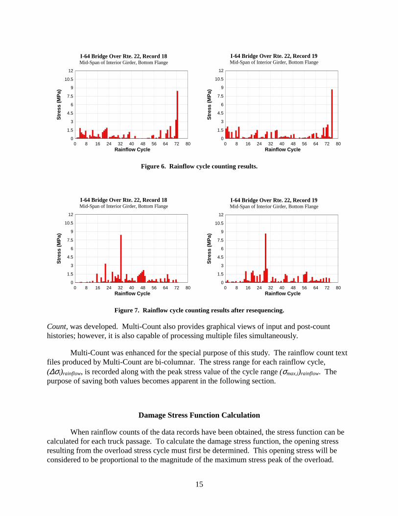
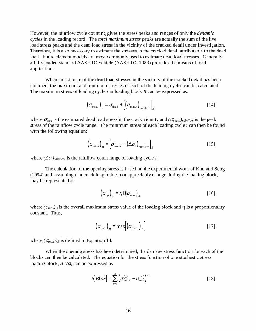
Figure 6 shows the results of the rainflow count of Records 18 and 19. Note that the largest cycle is counted last, which is characteristic of the algorithm. However, recall that the block loading model assumes that the opening stress is determined by the peak overload cycle, and the expression for the effective stress of the ith cycle in the block is given as

( ) ( )∆σ σ σeff i i op= −max . [13]

where (σmax)i are the stress ranges of the cycles subsequent to the overload. It is unclear from the rainflow output which cycles follow the overload and which ones come before it. Therefore, for the purposes of this study, a post-processing routine was written to resequence the rainflow count to give an indication of the time location of each of the stress cycles in the loading block. The resequenced rainflow counts of Records 18 and 19 are given in Figure7.

Cycle-Count performs the complete pre-processing, rainflow count, and post-processing of one stress cycle loading block. Cycle-Count is a 32-bit compliant program designed to run in the Microsoft Windows® environment. The user can save data files of the final counts or output a graph of the count to the clipboard or the Windows Print Manager.

When performing rainflow counts on a large number of data files, it would be inefficient to process the files one at a time. Therefore, an extended version of Cycle-Count, called Multi-

15

Rainflow Cycle

Stre

ss (M

Pa)


0 8 16 24 32 40 48 56 64 72 800

1.5

3

4.5

6

7.5

9

10.5

12

Rainflow Cycle

Stre

ss (M

Pa)


0 8 16 24 32 40 48 56 64 72 800

1.5

3

4.5

6

7.5

9

10.5

12

Figure 6. Rainflow cycle counting results.

Rainflow Cycle

Stre

ss (M

Pa)


0 8 16 24 32 40 48 56 64 72 800

1.5

3

4.5

6

7.5

9

10.5

12

Rainflow Cycle

Stre

ss (M

Pa)


0 8 16 24 32 40 48 56 64 72 800

1.5

3

4.5

6

7.5

9

10.5

12

Figure 7. Rainflow cycle counting results after resequencing.

Count, was developed. Multi-Count also provides graphical views of input and post-count histories; however, it is also capable of processing multiple files simultaneously.

Multi-Count was enhanced for the special purpose of this study. The rainflow count text files produced by Multi-Count are bi-columnar. The stress range for each rainflow cycle, (∆σi)rainflow, is recorded along with the peak stress value of the cycle range (σmax,i)rainflow. The purpose of saving both values becomes apparent in the following section.

Damage Stress Function Calculation

When rainflow counts of the data records have been obtained, the stress function can be calculated for each truck passage. To calculate the damage stress function, the opening stress resulting from the overload stress cycle must first be determined. This opening stress will be considered to be proportional to the magnitude of the maximum stress peak of the overload.

16

However, the rainflow cycle counting gives the stress peaks and ranges of only the dynamic cycles in the loading record. The total maximum stress peaks are actually the sum of the live load stress peaks and the dead load stress in the vicinity of the cracked detail under investigation. Therefore, it is also necessary to estimate the stresses in the cracked detail attributable to the dead load. Finite element models are most commonly used to estimate dead load stresses. Generally, a fully loaded standard AASHTO vehicle (AASHTO, 1983) provides the means of load application.

When an estimate of the dead load stresses in the vicinity of the cracked detail has been obtained, the maximum and minimum stresses of each of the loading cycles can be calculated. The maximum stress of loading cycle i in loading block B can be expressed as:

( ) ( )[ ]σ σ σmax, max,i B iB

= +dead rainflow [14]

where σdead is the estimated dead load stress in the crack vicinity and (σmax,i)rainflow is the peak stress of the rainflow cycle range. The minimum stress of each loading cycle i can then be found with the following equation:

( ) ( )[ ]σ σ σmin, max,i B i i B= − ∆

rainflow [15]

where (∆σi)rainflow is the rainflow count range of loading cycle i.

The calculation of the opening stress is based on the experimental work of Kim and Song (1994) and, assuming that crack length does not appreciably change during the loading block, may be represented as:

( ) ( )σ η σop B B= ⋅ max [16]

where (σmax)B is the overall maximum stress value of the loading block and η is a proportionality constant. Thus,

( ) ( )[ ]σ σmax max,maxB i B

= [17]

where (σmax,i)B is defined in Equation 14.

When the opening stress has been determined, the damage stress function for each of the blocks can then be calculated. The equation for the stress function of one stochastic stress loading block, B (ω), can be expressed as

( )[ ] ( ) ( )( )h B i

m

i

n

ω σ σω ω= −=� max, min

1 [18]

17

where m is the Paris law material exponent, n is the total number of rainflow cycles in B (ω) with a maximum stress peak greater than the calculated crack opening stress, and σmin

(ω) is defined as

σσ σ σσ σ σ

ωmin( ) min,

min, min,

=≥<

��

op op i

i op i

for for

[19]

Statistical Analysis of Damage Stress Functions

To estimate the detail reliability, a probability density function for the damage stress function must be found. Therefore, when the stress functions for the multiple truck passages have been calculated, a hypotheses must be made as to which probability distribution best represents the observed results and then the appropriate parameters estimated.

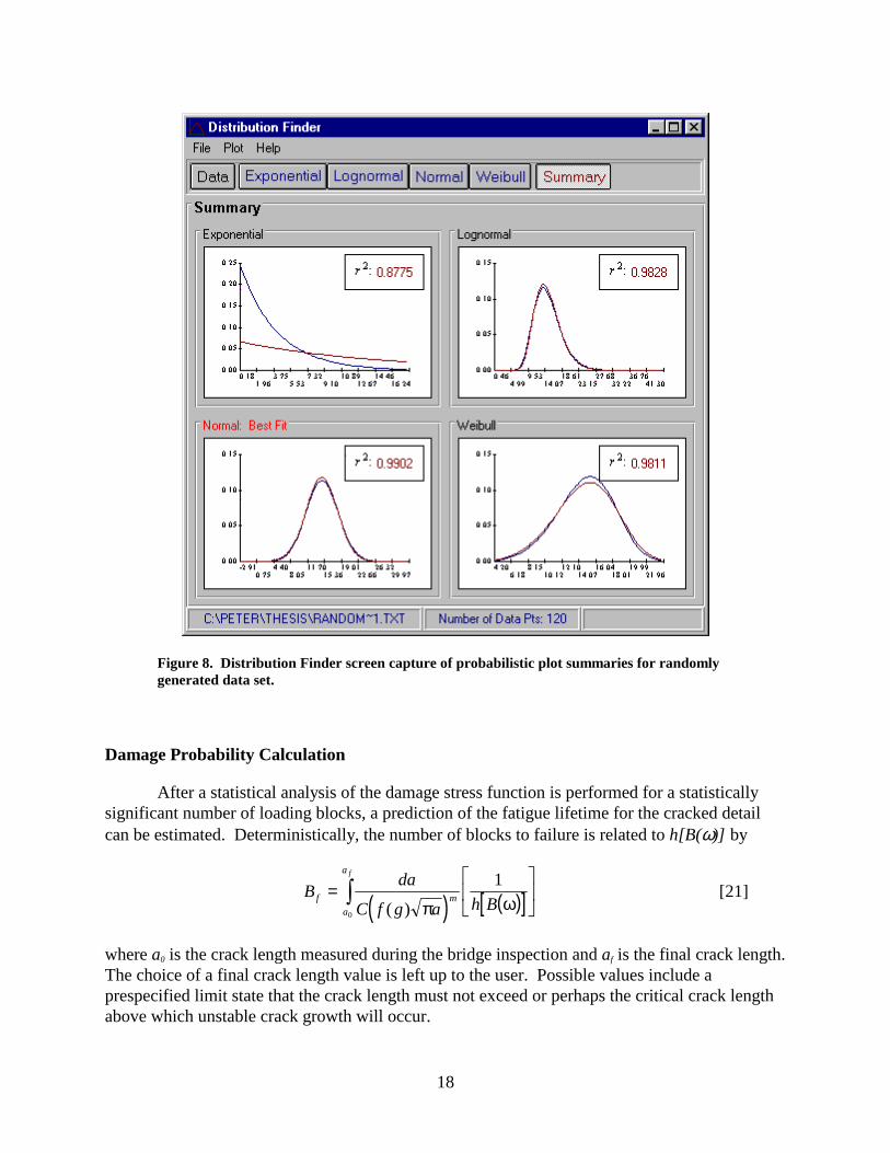
As a tool to accomplish the task of finding an appropriate distribution function for the damage stress block function, a program called Distribution Finder was developed. This program uses probability plotting techniques to determine how well a data set is represented by an exponential, normal, lognormal, or Weibull probability distribution.

When a data file is opened, Distribution Finder creates a histogram to approximate the expected probability density function (pdf) of the sample data. The stress intervals, ∆, for this plot are calculated with the following equation (Lewis, 1996):

( )[ ]∆ = +−

r N1 3 3 101

. log [20]

The method of least squares is used to define the line of best fit for each distribution, and the goodness of fit for each distribution is reported in terms of the coefficient of determination of the fitted lines. Based on this indicator, Distribution Finder suggests the most suitable probability distribution for each data file input by the user. Additionally, Distribution Finder calculates the parameter estimates for each distribution according to the method of weighted residuals and using the more sophisticated maximum likelihood methods and plots the pdfs for each distribution. Figure 8 shows the summary of each of the plots for a randomly generated data set. The normal distribution was chosen as the plot of best fit.

18

Figure 8. Distribution Finder screen capture of probabilistic plot summaries for randomly generated data set.

Damage Probability Calculation

After a statistical analysis of the damage stress function is performed for a statistically significant number of loading blocks, a prediction of the fatigue lifetime for the cracked detail can be estimated. Deterministically, the number of blocks to failure is related to h[B(ω)] by

( ) ( )[ ]B

da

C f g a h Bf ma

a f

=�

��

�

��

( ) π ω1

0

[21]

where a0 is the crack length measured during the bridge inspection and af is the final crack length. The choice of a final crack length value is left up to the user. Possible values include a prespecified limit state that the crack length must not exceed or perhaps the critical crack length above which unstable crack growth will occur.

19

However, to calculate the number of random blocks to failure, the damage stress function must be considered to be a random process. Due to the nonlinearity of the stress intensity factor, a closed form stochastic integration is difficult to obtain. However, recall that the crack growth per loading block equation for the proposed model was given as

( ) ( )[ ]∆∆

aB

C f g a h Bm

= ( ) π ω , [22]

This implies that the crack size after the jth loading block can be expressed as

( ) ( )[ ]a a C f g a h Bj j j j

m

j+ = +1 ( ) π ω . [23]

This stochastic difference equation provides an explicit expression for the crack length after the jth loading cycle given the crack length aj before the jth passage and the statistically independent value of the random h[B(ω)]. A closed form solution for aj+1 is difficult, since the coefficient multiplying h[B(ω)] is nonlinear in aj. However, numerous approximate solution techniques could be applied, including equivalent linearization and discrete closure techniques. Markov process models have also been developed, but the discrete formulation of Equation 11 does not appear to have been studied. In the present study, a somewhat more straightforward approach is used. An estimate of the statistics of the number of blocks to failure can be easily obtained by running a Monte Carlo simulation. This involves recursively calculating the crack size value aj+1 based on the previous crack size, aj, and a randomly generated value of h[Bj(ω)] for the jth truck crossing. This iteration is repeated until aj+1 ≥ af. When this condition is satisfied, block j is recorded as the failure block.

The simulation procedure must be repeated until enough Bf values have been generated to define accurately the random variation of the number of blocks to failure. The drawback of this method is the relatively large amount of computational time required to run the simulations. Typically, structural details exhibit high-cycle fatigue crack growth. Consequently, a crack of initial size a0 may not achieve its final state until it has been subjected to tens of millions of truck passages. This means that one simulation run would require this many iterations, and a distribution may not be reasonably assumed until more than 100 (and frequently more) simulations have been performed. However, an efficient and reasonable approximate method of performing the simulations was developed and is presented in the following subsection.

Modified Monte Carlo Simulation Using the Central Limit Theorem

As an introduction to this section, random number generation methods are briefly discussed. The randomly generated value of h[Bj(ω)] in Equation 23 must be drawn from a distribution of the same type and with the same parameters as those calculated for the damage stress block. (In other words, if the damage stress function is found to have a Weibull distribution with parameters θ and m, then, the random values of h[Bj(ω)] must be generated with a similar distribution.)

20

Papoulis (1991) suggested using the percentile transformation method of generating a Weibull distribution from uniformly distributed random numbers. Assuming that u is a sequence of random variables with a uniform distribution in the interval (0, 1), then

( )x F ui x i= −1 , [24]

is a random number sequence with cumulative distribution function Fx(x).

For a Weibull-distributed damage stress function H with a CDF of

F hh m

( ) exp= − −��

��

�

�

��1

θ, [25]

the random numbers

( )[ ]h ui im= − −θ ln 11

, [26]

have a Weibull distribution with parameters corresponding to those of the damage stress function, assuming ui is uniformly distributed between zero and one.

Ang and Tang (1984) presented the following formulae for generating normally distributed random numbers from two uniformly distributed random numbers, u1 and u2:

S U US U U

1 1 2

2 1 2

2 22 2

= −= −

ln( ) cos( )ln( ) sin( )

ππ

, [27]

where S1 and S2 are standard (µ = 0, σ = 1) normal random variables. Thus, a non-standard (µ = µns, σ = σ ns) normal random number xi can be generated with the relation

x Si ns i ns= +σ µ . [28]

Finally, for a lognormally distributed damage stress function h with a CDF of

F hhh

( ) ln=�

��

�

��

�

�

��Φ

1

0ω, [29]

the random number

21

( )h h Si i= 0 exp ω , [30]

has a lognormal distribution with parameters corresponding to those of the damage stress function.

Thus, if a statistical analysis reveals that the damage stress function for a particular detail has a Weibull or lognormal distribution, the single passage iteration procedure of Equation 23 can be performed using random numbers generated through the transformations expressed in Equation 14 or 18.

To reduce the computational demands of the single block iteration, the proposed model makes the following assumptions:

1. The crack size will remain reasonably constant over a period of consecutive, multiple

blocks so that there is no significant increase in the ( )C f g am

( ) π term of Equation 23 during this period.

2. The cumulative effect of multiple random values of the damage stress function can be

approximated by a single normally distributed random value by employing the central limit theorem (CLT) of probability.

Employing these assumptions allows the iterative crack growth equation to be rewritten as

( ) ( )[ ]a a C f g a h Bj N j N j

m

N+ = + ( ) π ω . [31]

where N is the number of blocks lumped into one iteration step, aj+N is the crack growth after each iteration step, and h[BN(ω)] is a normally distributed random value. This random value will be generated from a distribution with a mean of Nµh and a standard deviation of N hσ 2 , where µ h is the mean and σh

2 is the standard deviation of the damage stress function calculated from the stress histories recorded in the field.

Clearly, the validity of these assumptions is dependent upon the number of multiple blocks that will be lumped into one crack size iteration. The validity of applying the CLT is enhanced as N increases, but the constant crack size assumption is better for smaller N values. However, the CLT has been shown to be an extremely good approximation for the averaging of independent, identically distributed non-normal random variables. Thus, if N is chosen to correspond to the average daily truck traffic (ADTT) of the bridge (which is typically greater than 100), then the normal approximation is quite reasonable.

It would be extremely beneficial from a computational and analytical standpoint if the constant crack size assumption were also valid for an N value equivalent to the ADTT. This

22

assumption is the same as assuming that a crack in a bridge detail does not grow appreciably in one 24-hour period. Given the relatively large fatigue propagation lifetimes of most structural cracks, this assumption seems fairly reasonable. This assumption is analyzed next for a particular example, and it is shown that quite reasonable results are obtained.

Probability of Failure

When the Monte Carlo simulation has been run a statistically significant number of times, the blocks to failure, Bf, can be modeled as a random variable, Bf. The type of distribution that best describes this random variable can be evaluated using the probability plotting techniques described previously. Also, the parameters of this distribution can be estimated using maximum likelihood methods. Thus, the cumulative distribution frequency of Bf is given as

[ ]F n P nB ( ) = ≤B f . [32]

which represents the probability that the crack will grow to a size of af in n loading blocks.

Reliability Calculation

Equation 32 allows the estimation of the probability of failure for the detail with respect to the number of truck crossings. The reliability of the detail can then be readily calculated by employing the reliability definition:

R n F nB B( ) ( )= −1 . [33]

To calculate the reliability of the detail with respect to time, the rate of truck crossings can be either estimated using a deterministic function or modeled as a Poisson or other suitable arrival process.

If the single step iterative process of Equation 23 is employed, then the days to failure can be estimated by dividing the blocks to failure by the ADTT. However, if the multiple block iteration process of Equation 31 is used and N was taken to represent the ADTT, then the reliability can be expressed in terms of days directly. Further, if this method is employed, then the ADTT itself can be modeled as a random variable and easily included into the crack growth equation. Thus, the modified Monte Carlo simulation method can provide greater computational efficiency and the potential to incorporate directly other sources of randomness into the fatigue prediction. If suitable non-stationary models were available, for example, the ADTT could be modeled as a non-stationary (generally increasing) variable and a time to failure model that accounts for this increasing ADTT could be easily implemented. Alternately, if the material coefficients C and m in the underlying Paris’ law are allowed to vary randomly, this effect could be incorporated into the model with only minor increase in complication.

23

RESULTS AND DISCUSSION

Various aspects of the proposed model are examined in this section through the use of test data collected for two bridges. The greatest number of data records was recorded for the I-64 bridge over Route 22 in Shadwell, Virginia. Consequently, most of the data presented pertain to this bridge. Strain records were also recorded for the Route 29N bridge over the Robinson River in Madison County, Virginia. The live load strain ranges recorded for this bridge were generally greater in magnitude than those for the I-64 bridge. For this reason, the reliability calculations employ the damage stress block distribution function parameters estimated using the Route 29N data.

Damage Stress Function for Single Loading Block

It was shown previously that closure does not affect the damage stress block function when the following condition is met:

( ) ( )

( )ση σ σ

ηdead

i overload i overload>−

−max, min,

1 [34]

This is because the calculated opening stress falls below the minimum stress of each cycle in the loading block. So, when the effective stress intensity range is calculated, the minimum stress controls for every cycle in the loading block. The superimposed dead load effectively raises the R ratio for each cycle. Consequently, the effective stress range approaches the Paris law stress range as the dead load approaches the condition stated in Equation 34.

This relationship is shown in Figure 9 where the damage stress function is plotted versus the superposed dead load for a single loading block of the I-64 bridge. The damage stress function is shown for a range of η values. The peak stress of the overload rainflow count cycle for this loading block is 1.98 ksi, and the minimum stress for this load cycle is –0.35 ksi. Table 2 lists the limiting dead load stress of the closure region for the range of plotted η values. These values were calculated using Equation 34.

Figure 9 illustrates how the limiting dead load increases with η. The maximum damage stress function for the loading block is obtained when closure does not affect the crack growth. Thus, for each η value, the damage stress function reaches this maximum value at the dead load stresses corresponding to those given in Table 2. Although the opening-to-maximum stress ratio is unknown for structural steels, Newman (1995) has offered that η ranges from 0 to 0.7. Thus, for the load block shown in Figure 9, which is the most damaging load block recorded during the I-64 field tests, the crack growth of a detail in a region with a tensile dead load stress greater than 5.78 ksi can be predicted without employing closure considerations. Note that many fracture-critical bridge details are subjected to live stress ranges well below the dead load stress at their location. Consequently, closure effects will be negligible for these details. However, the closure considerations of the proposed model will prove most important when the dead load stresses fall

24

Dead Load Stress (ksi)

Dam

age

Stre

ss F

unct

ion

(ksi

)^m

0 2 4 6 8 100

1.5

3

4.5

6

7.5

9

10.5

12

13.5

15

Eta = 0.3Eta = 0.4Eta = 0.5Eta = 0.6Eta = 0.7Eta = 0.8

Figure 9. Damage stress function versus dead load stress for single loading block (σσσσmax,i = 1.98 ksi, σσσσmin,i = -0.35 ksi).

Table 2. Limiting dead load stresses for various ηηηη values for stress block with σσσσmax,i = 1.98 ksi snf σσσσmin,i = -0.35 ksi.

ηηηη Dead Load (ksi) 0.3 1.35 0.4 1.90 0.5 2.68 0.6 3.84 0.7 5.78 0.8 9.65

below the constraint given in Equation 34. This is evident from the sharply increasing curves shown in Figure 9.

Perhaps a better illustration of this is given in Figure 10 where the damage stress function is plotted versus η for dead load stresses of a magnitude similar to that of the live load stress ranges. The calculated damage stress function varies by an order of magnitude as η increases through the possible range of values for structural steels suggested by Newman (1995).

25

Eta

Dam

age

Stre

ss F

unct

ion

(ksi

)^m

0.3 0.4 0.5 0.6 0.7 0.80

1.5

3

4.5

6

7.5

9

10.5

12

13.5

15

Dead Load Stress = 0 ksiDead Load Stress = 1 ksiDead Load Stress = 2 ksi

Figure 10. Damage stress function versus opening:max stress ratio for single loading block (σσσσmax,i = 1.98 ksi, σσσσmin,i = -0.35 ksi).

Probabilistic Determination of Damage Stress Function for Multiple Loading Blocks

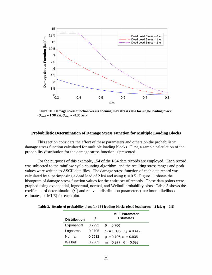
This section considers the effect of these parameters and others on the probabilistic damage stress function calculated for multiple loading blocks. First, a sample calculation of the probability distribution for the damage stress function is presented.

For the purposes of this example, 154 of the I-64 data records are employed. Each record was subjected to the rainflow cycle-counting algorithm, and the resulting stress ranges and peak values were written to ASCII data files. The damage stress function of each data record was calculated by superimposing a dead load of 2 ksi and using η = 0.5. Figure 11 shows the histogram of damage stress function values for the entire set of records. These data points were graphed using exponential, lognormal, normal, and Weibull probability plots. Table 3 shows the coefficient of determination (r2) and relevant distribution parameters (maximum likelihood estimates, or MLE) for each plot.

Table 3. Results of probability plots for 154 loading blocks (dead load stress = 2 ksi, ηηηη = 0.5)

Distribution

r2

MLE Parameter Estimates

Exponential 0.7992 θ = 0.706 Lognormal 0.9795 ω = 1.096, X0 = 0.412 Normal 0.5532 µ = 0.706, σ = 0.935 Weibull 0.9803 m = 0.977, θ = 0.698

26

Approximate PDF of Data

X

f(X)

0.0

0.2

0.4

0.6

0.8

0.01 1.11 2.21 3.30 4.40 5.50 6.60 7.70 8.80 9.90

Figure 11. Histogram of damage stress function values for 154 loading blocks (dead load stress = 2 ksi, ηηηη = 0.5).

Clearly, the damage stress functions do not fit the exponential or normal distributions well. The coefficients of determination for these two distributions are far below those of the lognormal and Weibull plots. The Weibull plot produced the greatest r2 value, but the data also fit the lognormal plot very well. Figures 12 and 13 show the probability plots for each of these distributions. One would expect the reliability calculation to produce similar results if the damage stress function was modeled using either distribution. The applicability of each of these distributions is discussed later.

Lognormal Plot

Omega = 1.096, X0 = 0.412 (R-Squared: 0.9795)

0

1

2

3

-1

-2

-3

-4

Figure 12. Lognormal plot of damage stress function for 154 loading blocks (dead load stress = 2 ksi, ηηηη = 0.5).

27

Weibull Plot

Shape = 0.977, Scale = 0.698 (R-Squared: 0.9803)

0

1

2

3

-1

-2

-3

-4

-5

-6

Figure 13. Weibull plot of damage stress function for 154 loading blocks (Dead load stress = 2 ksi, ηηηη = 0.5)

Effect of Dead Load Stress and Opening-To-Maximum Stress Ratio

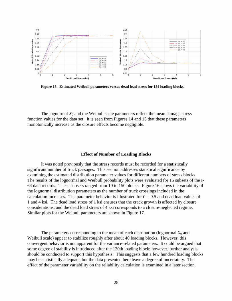
The damage stress functions were calculated for each of the 154 loading blocks for a range of dead load stress and η combinations. Again, high coefficients of determination were calculated for the lognormal and Weibull plots in every case. Figure 14 shows the variability of the lognormal parameters as the dead load stress increases for a range of η values. Figure 15 shows the results for the Weibull parameters. In all cases, as the dead load stress increases, the parameters approach the values estimated for the regime where closure has no effect. Note that the lognormal ω parameter and the Weibull shape parameter reflect the variance of the damage stress functions. Both parameters vary greatly with increasing opening-to-maximum stress ratios for dead load stresses between 0 and 2 ksi. This would be expected, because the dead load stresses in this range are comparable to the magnitude of the majority of overload cycles for the data set. Thus, closure effects introduce the greatest variability in the effective stress cycle ranges for these dead load values.


Logn

orm

al X

0 Pa

ram

eter

0 1 2 3 4 5 60

0.05

0.1

0.15

0.2

0.25

0.3

0.35

0.4

0.45

0.5

Eta = 0.3Eta = 0.4Eta = 0.5Eta = 0.6Eta = 0.7

Figure 14. Estimated lognormal parameters versus dead load stress for 154 loading blocks.

28


Wei

bull

Scal

e Pa

ram

eter

0 1 2 3 4 5 60

0.08

0.16

0.24

0.32

0.4

0.48

0.56

0.64

0.72

0.8



Wei

bull

Shap

e Pa

ram

eter

0 1 2 3 4 5 60.75

0.9

1.05

1.2

1.35

1.5

1.65

1.8

1.95

2.1

2.25


Figure 15. Estimated Weibull parameters versus dead load stress for 154 loading blocks.

The lognormal X0 and the Weibull scale parameters reflect the mean damage stress function values for the data set. It is seen from Figures 14 and 15 that these parameters monotonically increase as the closure effects become negligible.

Effect of Number of Loading Blocks

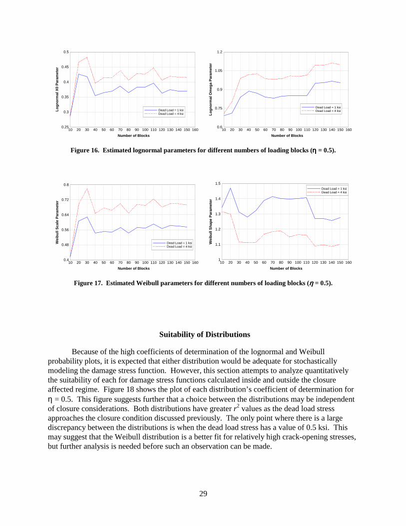
It was noted previously that the stress records must be recorded for a statistically significant number of truck passages. This section addresses statistical significance by examining the estimated distribution parameter values for different numbers of stress blocks. The results of the lognormal and Weibull probability plots were evaluated for 15 subsets of the I-64 data records. These subsets ranged from 10 to 150 blocks. Figure 16 shows the variability of the lognormal distribution parameters as the number of truck crossings included in the calculation increases. The parameter behavior is illustrated for η = 0.5 and dead load values of 1 and 4 ksi. The dead load stress of 1 ksi ensures that the crack growth is affected by closure considerations, and the dead load stress of 4 ksi corresponds to a closure-neglected regime. Similar plots for the Weibull parameters are shown in Figure 17.

The parameters corresponding to the mean of each distribution (lognormal X0 and Weibull scale) appear to stabilize roughly after about 40 loading blocks. However, this convergent behavior is not apparent for the variance-related parameters. It could be argued that some degree of stability is introduced after the 120th loading block; however, further analysis should be conducted to support this hypothesis. This suggests that a few hundred loading blocks may be statistically adequate, but the data presented here leave a degree of uncertainty. The effect of the parameter variability on the reliability calculation is examined in a later section.

29

Number of Blocks

Logn

orm

al X

0 Pa

ram

eter

10 20 30 40 50 60 70 80 90 100 110 120 130 140 150 1600.25

0.3

0.35

0.4

0.45

0.5

Dead Load = 1 ksiDead Load = 4 ksi

Number of Blocks

Logn

orm

al O

meg

a Pa

ram

eter

10 20 30 40 50 60 70 80 90 100 110 120 130 140 150 1600.6

0.75

0.9

1.05

1.2


Figure 16. Estimated lognormal parameters for different numbers of loading blocks (ηηηη = 0.5).

Number of Blocks

Wei

bull

Scal

e Pa

ram

eter

10 20 30 40 50 60 70 80 90 100 110 120 130 140 150 1600.4

0.48

0.56

0.64

0.72

0.8


Number of Blocks

Wei

bull

Shap

e Pa

ram

eter

10 20 30 40 50 60 70 80 90 100 110 120 130 140 150 1601

1.1

1.2

1.3

1.4

1.5Dead Load = 1 ksiDead Load = 4 ksi

Figure 17. Estimated Weibull parameters for different numbers of loading blocks (ηηηη = 0.5).

Suitability of Distributions

Because of the high coefficients of determination of the lognormal and Weibull probability plots, it is expected that either distribution would be adequate for stochastically modeling the damage stress function. However, this section attempts to analyze quantitatively the suitability of each for damage stress functions calculated inside and outside the closure affected regime. Figure 18 shows the plot of each distribution’s coefficient of determination for η = 0.5. This figure suggests further that a choice between the distributions may be independent of closure considerations. Both distributions have greater r2 values as the dead load stress approaches the closure condition discussed previously. The only point where there is a large discrepancy between the distributions is when the dead load stress has a value of 0.5 ksi. This may suggest that the Weibull distribution is a better fit for relatively high crack-opening stresses, but further analysis is needed before such an observation can be made.

30


Coe

ff. o

f Det

erm

inat

ion

0.5 1 1.5 2 2.5 3 3.50.92

0.94

0.96

0.98

1

LognormalWeibull

Figure 18. Lognormal and Weibull probability plot coefficients of determination for different dead load stresses.

Sample Reliability Prediction Using Collected Data

To evaluate the proposed model, a sample reliability calculation was performed for a cracked detail studied by Fisher (1984). This detail was present in the Ft. Duquesne bridge in Pittsburgh. A number of through cracks were discovered in the corners of a steel box girder. One of the cracks in the cross-girder beam tension flange exhibited signs of fatigue crack growth. Fisher proposed the following stress intensity equation to model the detail:

K aat f

=�

��

�

��

�

�

��

�

�

��

1122

. secσ ππ

[35]

where tf is the flange thickness (2.5 in). The initial crack size was measured to be 1.8 in, and the crack extension attributable to fatigue was approximately 0.15 in.

Fisher (1984) assumed the effective stress range in the vicinity of the crack to be 2 ksi. He also assumed that the actual crack extension occurred during the service life of the bridge (10 years). By employing ADTT estimates, he suggested that this corresponded to about 1.5 million truck crossings. The dead load stress in the flange was estimated to be 32 ksi. The flange material was A517 steel, and Fisher (1984) used Paris’ law constant values of C = 3.6 x 10-10 and m = 3 for his crack growth (inches) prediction that was based on stress intensity factor units of ksi⋅in½. These values are equivalent to those reported by Barsom and Rolfe (1987) for ferrite-pearlite steels.

31

As stated previously, the Route 29N bridge data exhibited stress ranges of a slightly greater magnitude than those recorded for the I-64 bridge. Therefore, the damage stress block distribution for this example was calculated using these data. The rationale behind this choice was that the effective stress ranges for these data are closer to those estimated by Fisher (1984). However, a precise comparison would require detailed knowledge of the stress cycles of the Ft. Duquesne bridge.

The damage stress function of the Route 29N bridge is best modeled as a lognormal random variable. The maximum likelihood parameter estimates for this distribution were calculated to be ω = 1.346 and x0 = 1.238. For a dead load stress in the non-closure affected regime, the reliability was calculated using Fisher’s stress intensity factor equation and Paris’ law constants.

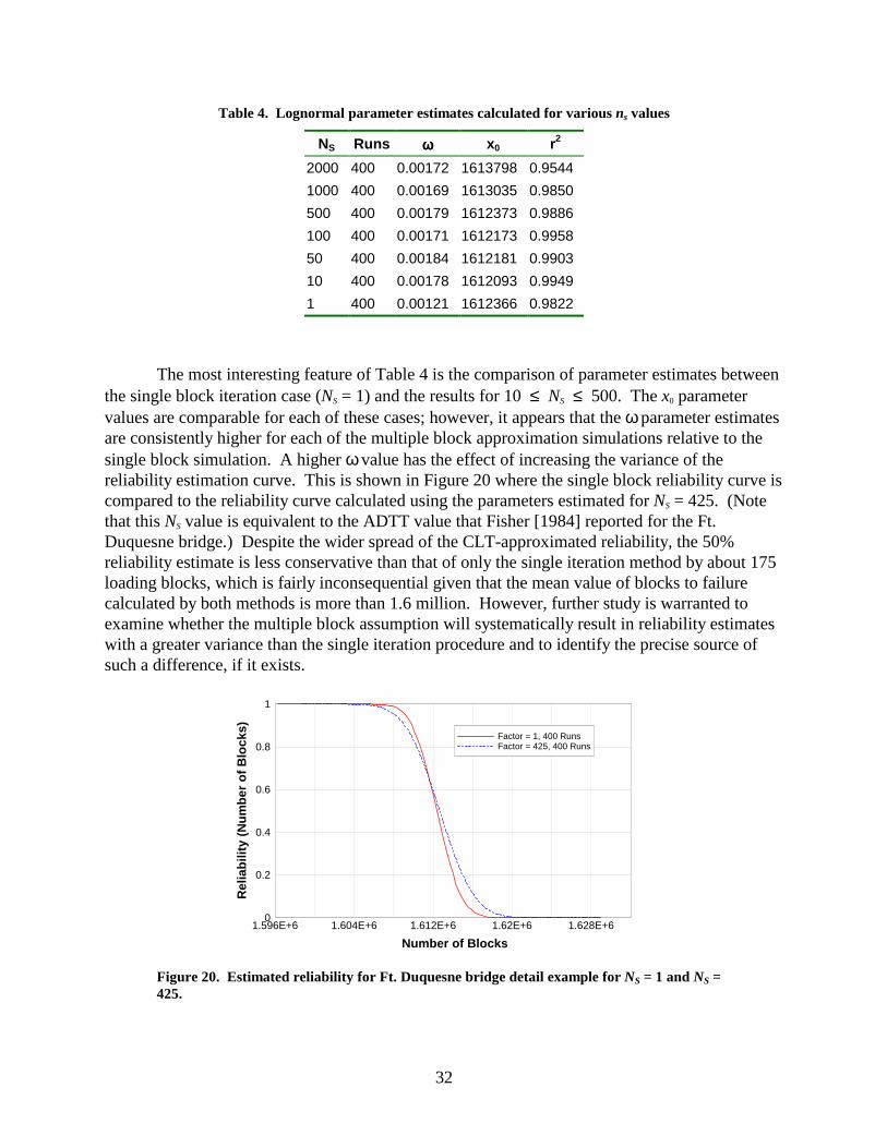
To evaluate the modified Monte Carlo method, numerous simulations were run using different values for the iteration step, NS. For each value of NS, 400 simulations were run to model the distribution of blocks to failure. For each series of simulations, the randomness of Bf was best described by a lognormal distribution. The resulting lognormal parameters estimated for each value of NS are given in Table 4. The simulations run for NS = 1 were generated using the lognormal parameters calculated for the damage stress function. All other simulations (NS > 1) were generated using the CLT approximation described previously.

All parameter estimates for NS values between 10 and 500 appear to be fairly close; however, the x0 parameter estimates for NS values greater than 500 are slightly larger. The effect of this difference in x0 values can be seen in Figure19, which shows the results of the detailed reliability calculation based on the parameters calculated when NS = 2000, 1000, 500, 100, and 10. The reliability curves for the three lower values are virtually identical, but the curves for NS > 500 appear to start shifting to the right. This suggests that the assumption concerning negligible crack growth for NS loading blocks begins to deteriorate when NS surpasses a particular value (in this case, about 0.03% of the fatigue life). This value is most likely dependent on the ratio of NS to the estimated average number of blocks required to exceed the final crack size for a given a0.

Number of Blocks

Rel

iabi

lity

(Num

ber o

f Blo

cks)

1.596E+6 1.604E+6 1.612E+6 1.62E+6 1.628E+60

0.2

0.4

0.6

0.8

1

Factor = 2000Factor = 1000Factor = 500Factor = 100Factor = 10

Figure 19. Estimated reliability for Ft. Duquesne bridge detail.

32

Table 4. Lognormal parameter estimates calculated for various ns values

NS Runs ωωωω x0 r2 2000 400 0.00172 1613798 0.9544 1000 400 0.00169 1613035 0.9850 500 400 0.00179 1612373 0.9886 100 400 0.00171 1612173 0.9958 50 400 0.00184 1612181 0.9903 10 400 0.00178 1612093 0.9949 1 400 0.00121 1612366 0.9822

The most interesting feature of Table 4 is the comparison of parameter estimates between the single block iteration case (NS = 1) and the results for 10 ≤ NS ≤ 500. The x0 parameter values are comparable for each of these cases; however, it appears that the ω parameter estimates are consistently higher for each of the multiple block approximation simulations relative to the single block simulation. A higher ω value has the effect of increasing the variance of the reliability estimation curve. This is shown in Figure 20 where the single block reliability curve is compared to the reliability curve calculated using the parameters estimated for NS = 425. (Note that this NS value is equivalent to the ADTT value that Fisher [1984] reported for the Ft. Duquesne bridge.) Despite the wider spread of the CLT-approximated reliability, the 50% reliability estimate is less conservative than that of only the single iteration method by about 175 loading blocks, which is fairly inconsequential given that the mean value of blocks to failure calculated by both methods is more than 1.6 million. However, further study is warranted to examine whether the multiple block assumption will systematically result in reliability estimates with a greater variance than the single iteration procedure and to identify the precise source of such a difference, if it exists.

Number of Blocks

Rel

iabi

lity

(Num

ber o

f Blo

cks)

1.596E+6 1.604E+6 1.612E+6 1.62E+6 1.628E+60

0.2

0.4

0.6

0.8

1

Factor = 1, 400 RunsFactor = 425, 400 Runs

Figure 20. Estimated reliability for Ft. Duquesne bridge detail example for NS = 1 and NS = 425.

33

The multiple loading block assumption allows a reliability estimate to be obtained with significantly less computational effort. than the single-loading block procedure. The single block iteration method is quite time-consuming for most realistic crack growth estimates. The curves generated in Figure 20 were based on parameter estimates obtained through 400 simulation runs. These simulations were run on a Pentium 133 MHz-based PC. The simulation program was written in Visual Basic� 4.0 with 32-bit Microsoft Foundation Class object controls. The total run time for the multiple block iteration calculations was approximately 1 minute and 7 seconds, whereas it took more than 8 hours to run the single block iterations.

To evaluate how many simulation runs are necessary to ensure a reasonable convergence of the parameter estimates, 1,000 simulation runs were conducted with the multiple block assumption and an ADTT of 425. Table 5 shows the resulting MLE parameter estimates calculated for the simulations and their various subsets. There is little appreciable difference between the parameters calculated for 100 runs and those calculated for 1,000 runs. This is evidenced by Figure 21, which shows the reliability curves based on the parameter estimates for 100, 500, and 1,000 runs.

Table 5. Lognormal parameter estimates calculated using different number of simulation runs for ns = 425.

ADTT Runs w X0 r2 425 1000 0.00178 1612613 0.996 425 500 0.00182 1612419 0.9967 425 400 0.00171 1612661 0.9956 425 300 0.00176 1612229 0.995 425 200 0.00180 1612127 0.9902 425 100 0.00167 1612541 0.9776

Number of Blocks

Rel

iabi

lity

(Num

ber o

f Blo

cks)

1.596E+6 1.604E+6 1.612E+6 1.62E+6 1.628E+60

0.2

0.4

0.6

0.8

1

Factor = 425, 1000 RunsFactor = 425, 500 RunsFactor = 425, 100 Runs

Figure 21. Estimated reliability for Ft. Duquesne bridge detail example based on different number of simulation runs for NS = 425.

34

Comparison of Model with Alternatives

Reliability estimates were calculated for the previous example using two methods commonly employed in bridge fatigue studies. One method calculates damage based only on the cycle greatest stress range for each stress block. The other employs Barsom’s (1973) RMS method where the effective stress range is taken to be the RMS of the peak stress ranges of the spectra samples.

Peak Cycle Only Analysis

In the study of bridge fatigue, it is common to assume that each truck passage produces only a single damaging stress range. This range is taken to be the greatest observed stress range in the loading block. Through this assumption, the block loading crack growth equation can be expressed as

( )∆∆

∆σaB

C f g am

= ( ) maxπ , [36]

where ∆σmax is the maximum stress cycle range observed in the random stress block, B. To calculate the reliability of a bridge detail, assuming single cycle damage, ∆σmax

m must be modeled as a random variable.

For the Route 29N bridge data, probability plotting techniques suggest that this random variable is lognormally distributed (r2 = 0.9841) with MLE parameters of ω = 1.537 and x0 = 0.396.

To compare the reliability estimate of the proposed model with commonly used fatigue prediction methods, the distribution of ∆σmax

m was also calculated for only the loading blocks with a peak cycle range greater than 1 ksi. About 30% of the stress histories recorded for the Route 29N bridge had peak cycle ranges above this value; consequently, this is referred to as the 30% peak cycle method. The lognormal parameter estimates of the peak cycle damage function using this criterion were ω = 0.669 and x0 = 2.860.

Because this latter distribution is based on a subset of the total truck crossings, it is informative to translate the block-based reliability to a rough approximation of the reliability with respect to time. This approximation involves dividing the blocks to failure for the damage stress block method and the total peak cycle method by the ADTT. However, assuming that 30% of the ADTT will produce peak cycle ranges greater than 1 ksi, the 30% peak cycle reliability values are divided by 0.3 times the ADTT.

Table 6 shows the approximate times to failure corresponding to a reliability value of 0.5 as calculated by the proposed method and each of the peak cycle methods. Note that the peak cycle estimates are greater than that of the proposed model. This means that slower crack growth is being predicted by the peak-cycle-only models. This is because the proposed model also takes

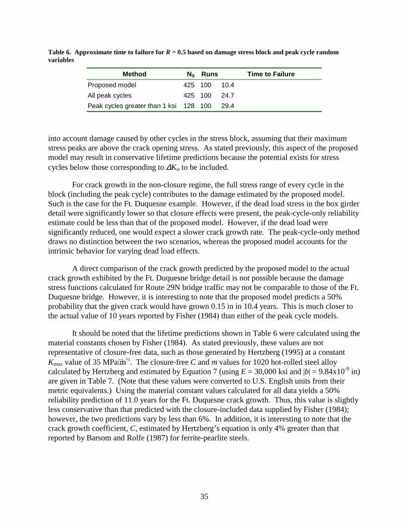
35

Table 6. Approximate time to failure for R = 0.5 based on damage stress block and peak cycle random variables

Method NS Runs Time to Failure Proposed model 425 100 10.4 All peak cycles 425 100 24.7 Peak cycles greater than 1 ksi 128 100 29.4

into account damage caused by other cycles in the stress block, assuming that their maximum stress peaks are above the crack opening stress. As stated previously, this aspect of the proposed model may result in conservative lifetime predictions because the potential exists for stress cycles below those corresponding to ∆Kth to be included.

For crack growth in the non-closure regime, the full stress range of every cycle in the block (including the peak cycle) contributes to the damage estimated by the proposed model. Such is the case for the Ft. Duquesne example. However, if the dead load stress in the box girder detail were significantly lower so that closure effects were present, the peak-cycle-only reliability estimate could be less than that of the proposed model. However, if the dead load were significantly reduced, one would expect a slower crack growth rate. The peak-cycle-only method draws no distinction between the two scenarios, whereas the proposed model accounts for the intrinsic behavior for varying dead load effects.

A direct comparison of the crack growth predicted by the proposed model to the actual crack growth exhibited by the Ft. Duquesne bridge detail is not possible because the damage stress functions calculated for Route 29N bridge traffic may not be comparable to those of the Ft. Duquesne bridge. However, it is interesting to note that the proposed model predicts a 50% probability that the given crack would have grown 0.15 in in 10.4 years. This is much closer to the actual value of 10 years reported by Fisher (1984) than either of the peak cycle models.

It should be noted that the lifetime predictions shown in Table 6 were calculated using the material constants chosen by Fisher (1984). As stated previously, these values are not representative of closure-free data, such as those generated by Hertzberg (1995) at a constant Kmax value of 35 MPa⋅m½. The closure-free C and m values for 1020 hot-rolled steel alloy calculated by Hertzberg and estimated by Equation 7 (using E = 30,000 ksi and |b| = 9.84x10-9 in) are given in Table 7. (Note that these values were converted to U.S. English units from their metric equivalents.) Using the material constant values calculated for all data yields a 50% reliability prediction of 11.0 years for the Ft. Duquesne crack growth. Thus, this value is slightly less conservative than that predicted with the closure-included data supplied by Fisher (1984); however, the two predictions vary by less than 6%. In addition, it is interesting to note that the crack growth coefficient, C, estimated by Hertzberg’s equation is only 4% greater than that reported by Barsom and Rolfe (1987) for ferrite-pearlite steels.

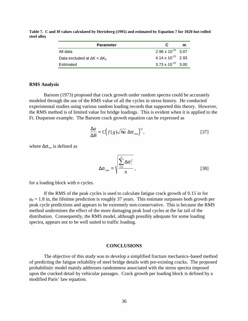
36

Table 7. C and M values calculated by Hertzberg (1995) and estimated by Equation 7 for 1020 hot-rolled steel alloy

Parameter C m All data 2.96 x 10-10 3.07 Data excluded at ∆K < ∆Kb 4.14 x 10-10 2.93 Estimated 3.73 x 10-10 3.00

RMS Analysis

Barsom (1973) proposed that crack growth under random spectra could be accurately modeled through the use of the RMS value of all the cycles in stress history. He conducted experimental studies using various random loading records that supported this theory. However, the RMS method is of limited value for bridge loadings. This is evident when it is applied to the Ft. Duquesne example. The Barsom crack growth equation can be expressed as

( )∆∆

∆σaB

C f g a rms

m= ( ) π , [37]

where ∆σrms is defined as

∆σ∆σ

rms

ii

n

n= =

� 2

1 , [38]

for a loading block with n cycles.

If the RMS of the peak cycles is used to calculate fatigue crack growth of 0.15 in for a0 = 1.8 in, the lifetime prediction is roughly 37 years. This estimate surpasses both growth per peak cycle predictions and appears to be extremely non-conservative. This is because the RMS method undermines the effect of the more damaging peak load cycles at the far tail of the distribution. Consequently, the RMS model, although possibly adequate for some loading spectra, appears not to be well suited to traffic loading.

CONCLUSIONS

The objective of this study was to develop a simplified fracture mechanics–based method of predicting the fatigue reliability of steel bridge details with pre-existing cracks. The proposed probabilistic model mainly addresses randomness associated with the stress spectra imposed upon the cracked detail by vehicular passages. Crack growth per loading block is defined by a modified Paris’ law equation.

37

When a bridge inspection reveals the existence of fatigue cracks, field data in the form of strain measurements can be collected in the vicinity of the fracture detail to identify the characteristic stress block and the fluctuations in the curve attributes attributable to randomness of the traffic loading.

The following conclusions are drawn from the analytical formulation of the model and its application to loading spectra recorded in the field:

• The damage stress function can be probabilistically defined through the statistical analysis of the stress block functions calculated for random truck passages. Two-parameter probability distributions appear adequate to describe the stress functions calculated from measured field data. For the bridge details instrumented in this study, the damage stress function can be modeled as a Weibull or lognormal random variable.

• The mean-associated parameter estimate for each of these distributions shows signs of convergence for as few as 40 stress record samples. A trend toward convergence for the variance-associated parameters was less obvious; however, for each distribution, the maximum fluctuation between 40 and 150 samples was less than 10%.

• For high-cycle, slow growth damage that is characteristic of bridge fatigue, an approximation of reliability distribution parameters can be obtained by assuming negligible daily crack growth and approximating the summation of stochastic damage stress block functions as a normal random variable. A reliability estimate using this assumption was comparable to that of a single passage estimate, and computational savings were significant.

RECOMMENDATIONS FOR FUTURE RESEARCH

The proposed model focuses on randomness associated with the loading spectra. The low level of variance obtained for the reliability estimate of the Ft. Duquesne bridge detail suggests that the resistance variables may have the most significant effect on the randomness of the reliability prediction and, therefore, should be included in future models. Specifically, the initial crack size and Paris’ law constants can be modeled as random factors and directly substituted into Equation 19. Random material variations may occur from point to point within a specimen, as well as between specimens. Limited data are available for this model extension using structural steel, although somewhat more data exist for typical aerospace materials. However, Itagaki et al. (1993) developed an experimental paradigm for determining the probability distribution functions of the Paris law material constants and reported results for a high tensile strength steel. The inclusion of other random variables may necessitate a greater number of simulation runs to model the reliability distribution; however, the multiple block approximation makes this computationally feasible.

38

Further consideration should be given to developing a viable method of verifying the proposed model. Perhaps a laboratory simulation could be performed to measure crack growth in a typical fatigue-critical detail subjected to programmed loading spectra equivalent to those recorded in the field. Alternatively, an accelerated fatigue evaluation could be made in the field by constructing a cracked detail specimen and attaching it to an in-situ structure. For instance, a finite-width center cracked specimen could be fabricated and bolted onto a girder flange. This detail will be subjected to actual vehicular loading spectra, yet it will not be structurally critical. The crack growth could then be monitored over a period of time and measurements could be taken for comparison with the model prediction.

The model might also be suitable as a tool in design analysis of critical bridge details, provided suitable stress time histories could be simulated. This might entail numerical models of structures together with random models of vehicular speed, axle weights, and road roughness. Initial reliability projections could be enhanced by data on distribution of initial flaws sizes in details of various types. The method could also be used, given field data, but no known flaws, to predict likely evolution of cracks, based on distributions of initial flaws sizes. Data are needed to predict the distribution of those flaw sizes.

ACKNOWLEDGMENTS

This study was funded by the Federal Highway Administration. The authors are grateful for the support and assistance of this organization.

REFERENCES American Association of State Highway and Transportation Officials. (1983). Standard

Specifications for Highway Bridges, 13th Edition. Washington, D.C. American Association of State Highway and Transportation Officials. (1989). Guide

Specifications for Fatigue of Steel Bridges, 13th Edition. Washington, D.C. Ang, A. S. H. & Tang, W. H. (1984). Probability Concepts in Engineering Planning and

Design, Vol. 2. New York: John Wiley & Sons. Bannantine, J. A., Comer, J. J. & Handrock, J. L. (1990). Fundamentals of Metal Fatigue

Analysis. Englewood Cliffs, NJ: Prentice-Hall. Barsom, J. M. (1973). Fatigue-Crack Growth Under Variable Amplitude Loading in ASTM

A514 Grade B Steel. (ASTM STP 536). Philadelphia: American Society for Testing and Materials.

Barsom, J. M. & Rolfe, S. T. (1987). Fracture and Fatigue Control in Structures. (2nd

Edition). Englewood Cliffs, NJ: Prentice-Hall.

39

Barsom, J. M. & Novak, S. R. (1977). Subcritical Crack Growth and Fracture of Bridge Steels. National Cooperative Highway Research Program Report 181. Washington, DC: Transportation Research Board.

Brussat, T. R. (1974). Rapid Calculation of Fatigue Crack Growth by Integration. In Fracture

Toughness and Slow-Stable Cracking, pp. 298-311. (ASTM STP 559). Philadelphia: American Society for Testing and Materials.

Committee on Fatigue and Fracture Reliability of the Committee on Structural Safety and

Reliability of the Structural Division. (1982). Fatigue Reliability: Introduction. Journal of the Structural Division, 108(ST1): 3-24.

Downing, S. D., & Socie, D. F. (1982). Simplified Rainflow Counting Algorithms.

International Journal of Fatigue, 4(1): 31-40. Elber, W. (1971). The Significance of Crack Closure. In Damage Tolerance in Aircraft

Structures. (ASTM STP 486). Philadelphia: American Society for Testing and Materials.

Fisher, J. W. (1984). Fatigue and Fracture in Steel Bridges. New York: John Wiley & Sons,

Inc. Fisher, J. W. & Yuceoglu, U. (1981). A Survey Of Localized Cracking In Steel Bridges, Interim

Report. (DOT-FH-11-9506). Washington, DC: Federal Highway Administration. Hoadley, P. W., Frank, K. H., & Yura, J. A. (1983). Estimation of the Fatigue Life of a Test

Bridge from Traffic Data. (Research Report 247-4). Austin: Center for Transportation Research, Bureau of Engineering Research, University of Texas.

Irwin, G. R. (1957). Analysis Of Stresses And Strains Near The End Of A Crack Traversing A

Plate. Journal of Applied Mechanics, Vol. E24, p. 361. Itagaki, H., Ishizuka, T. & Yan, H. P. (1993). Experimental Estimation of the Probability

Distribution of Fatigue Crack Growth Lives. Probabilistic Engineering Mechanics, 8: 25-34.

Kim, C. Y. & Song, J. H. (1994). Fatigue Crack Closure And Growth Behavior Under Random

Loading. Engineering Fracture Mechanics, 49(1): 105-120. Lewis, E. E. (1996). Introduction to Reliability Engineering. (2nd ed.). New York: John Wiley

& Sons, Inc. Melchers, R. E. (1987). Structural Reliability: Analysis and Prediction. Chichester, England:

Ellis Horwood Ltd.

40

Newman, Jr., J. C. (1995). Fatigue Life Prediction Methodology Using a Crack-Closure Model. Journal of Engineering Materials and Technology, 117, 433-439.

Papoulis, A. (1991). Probability, Random Variables, and Stochastic Processes. (3rd ed.). New

York: McGraw-Hill, Inc. Paris, P. C. & Erdogan, F. (1963). A Critical Analysis of Crack Propagation Laws. Journal of

Basic Engineering, D85: 528-53. Paris, P. C., Gomez, M. P. & Anderson, W. E. (1961). A Rational Analytic Theory of Fatigue.

The Trend in Engineering, 13(1): 9-14. Sunder, R. (1992). Near-Threshold Fatigue Crack Growth Prediction Under Spectrum Loading.

In Advances in Fatigue Lifetime Predictive Techniques, pp. 161-175. (ASTM STP 1122). Philadelphia: American Society for Testing and Materials.

Tang, J. & Spencer, B. F., Jr. (1989). Reliability Solution for the Stochastic Fatigue Crack

Growth Problem. Engineering Fracture Mechanics, 34(2): 419-433. Tao, Z., Ellis, H. & Corotis, R. B. (1995). Structural Reliability Evaluation With Maintenance

Actions: Restructuring: America and Beyond. In M. Sanayei, Ed., Proceedings of Structures Congress XIII, pp. 599-602. Boston: American Society of Civil Engineers.

Xanthakos, P. P. (1994). Theory and Design of Bridges. New York: John Wiley and Sons. Zhao, Z., Haldar, A. & Breen Jr., F. L. (1994a). Fatigue-Reliability Evaluation of Bridges.

Journal of Structural Engineering, 120(5): 1608-1623. Zhao, Z., Haldar, A. & Breen Jr., F. L. (1994b). Fatigue-Reliability Updating through

Inspections of Steel Bridges. Journal of Structural Engineering, 120(5): 1624-1642.

FINAL REPORT FATIGUE RELIABILITY OF STEEL … fracture failure subsequent to fatigue cracking is the...

Documents

Transcript of FINAL REPORT FATIGUE RELIABILITY OF STEEL … fracture failure subsequent to fatigue cracking is the...