FARADAY TRANS., 1990, 86(10), How Wrong is the Debye ... · How Wrong is the Debye-Huckel...
29
J. CHEM. SOC. FARADAY TRANS., 1990, 86(10), 1815-1843 1815 How Wrong is the Debye-Huckel Approximation for Dilute Primitive Model Electrolytes with Moderate Bjerrum Parameter? Torben Smith Serensen Fysisk-Kemisk lnstitut and Center for Modellering, lkke-lineare systemers Dynamik og lrreversibel Termodynamik (MIDIT), Technical University of Denmark, Bldg. 206, DK-2800 Lyngby, Denmark ~~ ~~~ ~ ~ Monte Carlo (MC) simulations have been performed for primitive model electrolytes for moderate Bjerrum parameters (B = 1, B = 1.546 and a few with B = 1.681) and values of m in the range ca. 0.015-0.45. Emphasis has been laid on very dilute systems. Several millions of configurations have been used, and the number of ions in each simulation (N) was varied between N = 32 and N = 1000 (N = 1728 in a single case). It is shown, by means of 'universal scaling' comparing the Debye length l/rc with the periodic length of the boundary condi- tions, that excess energies (€,,/NkT) should be extrapolated using a polynomial commencing with the power 3 in 1/N rather than the usual plots against 1/N. The same seems to be the case for the electrostatic, excess Helmholtz free energy and the excess heat capacity. However, the logarithm of the activity coefficients (Iny., In y + and In y-) as calculated by the test particle method of Widom should be extrapolated with a leading term, which is the cube root of 1/N. The extrapolated values of the thermodynamic parameters compare well with high-precision HNC calculations and with DHX calculations. In summary, the conclusion is drawn, that the usual Debye-Huckel laws (including the m correction) and not the Debye-Huckel limiting laws are the true low-correlation limits (limit of low plasma parameter Bm) for the electrostatic contributions to the thermodynamic properties. However, even for 1 : 1 electrolytes there are small, but significant deviations from the DH laws. These deviations increase with B. For the excess heat capacity, the deviations are quite large. They are predicted accurately by the DHX approx- imation. A consistency check has been made of the DHX theory, calculating In yi in various ways. This model is quite consistent at low values of m, when we depart from E,, , but less consistent when using the Kirkwood-Buff formalism, dependent on the second moment with respect to the radial distance of the radial distribution func- tions. The Monte Carlo results for the radial distribution functions are statistically indistinguishable from the DHX radial distribution functions. Also, the DHX and the HNC radial distribution functions cannot be distinguished up to at least m = 0.45. For unequal radii of the ions, a straightforward generalisation of DHX (GDHX) is found to hold true comparing with MC simulations. The thermodynamic properties in dilute systems are dominated by the contact distance between the cation and the anion. Fixing this (B = 1.546), and increasing the ratio between the radii of the two ions to 3 leads to quite small, though systematic changes in the thermodynamic properties at ~a =ca. 0.10 and 0.14. In particular, one observes that Iny, = Iny- = Iny, to a very good approximation, at least for this dilute system. 1. Introduction The primitive model (PM) of electrolytes (ions of different sizes in a dielectric continuum) is still a fascinating study area in statistical mechanics, since it involves a delicate balance between the very far-reaching Coulombic forces and the extremely short-range ' hard-sphere ' forces. The classical for- mulae of Debye and Huckel (DH)' for the thermodynamic properties of a mixture of ions with equal sizes (the restricted primitive model, RPM) represented an important step forward compared with the ambitious, but largely unsuc- cessful, earlier attempt of Milner2*3 to calculate the configu- ration integral in a more direct manner. However, a high price was paid in terms of approximations, the exact meaning of which have worried electrochemists and statistical mecha- nicists ever since. Already in 1926, Kramers4 returned to the problem of a direct determination of the configuration integral in dilute primitive electrolytes. In spite of a number of new and elegant methods introduced to solve the problem, for example a technique for removing the Coulombic singularity for point charges and the consideration of the ionic charges as stochastic variables (!), Kramers concluded, that 'a com- parison of the theory with the experiments is rather useless so long as the influence of the ionic radii has not been investi- gated more closely'. Much later, RCsibois5 could state that 'unfortunately, the considerable effort which has been put into this problem has not resulted in much interest. No rigor- ous theory is presently available beyond the limiting law region'. Rbibois was referring to a derivation of the limiting law by means of the BBGKY hierarchy of equations and also the derivation by Mayer6 by ring graph summation. However, several advances have occurred in the latest 20 years. First of all, a number of Monte Carlo (MC) studies of the primitive model have appeared following the pioneering studies of P ~ i r i e r , ~ Vorontsov-Vel'yaminov et dgV9 and Card and Valleau.'O Secondly, the 'hypernetted chain' (HNC) integral-equation approximation has proved to be very effi- cient to reproduce closely the MC 'data' for PM electrolytes with moderate Bjerrum parameters."-'4 An even simpler integral-equation approach is the mean spherical approximation (MSA).l5-I8 This approximation leads to analytical results for the thermodynamic funcions of the RPM, and the formulae are isomorphous with the simple DH formulae apart from a generalisation of the Debye shielding length. However, the radial distribution functions close to contact are bad, especially for dilute systems. Fur- thermore, the MSA values for the thermodynamic functions are identical to the DH results for low electrolyte concentra- tions. Thus, the first deviation from the Debye-Huckel limit- ing law (DHLL) predicted by the MSA theory is just as inconsistent as the 'contact distance correction' in the clas- sical DH theory. Indeed, compared with existing MC data, the MSA theory appears to be best for moderate concentra- tions of 1 : 1 electrolytes. However, the HNC approximation
Transcript of FARADAY TRANS., 1990, 86(10), How Wrong is the Debye ... · How Wrong is the Debye-Huckel...

J. CHEM. SOC. FARADAY TRANS., 1990, 86(10), 1815-1843 1815
How Wrong is the Debye-Huckel Approximation for Dilute Primitive Model Electrolytes with Moderate Bjerrum Parameter?
Torben Smith Serensen Fysisk-Kemisk lnstitut and Center for Modellering, lkke-lineare systemers Dynamik og lrreversibel Termodynamik (MIDIT), Technical University of Denmark, Bldg. 206, DK-2800 Lyngby, Denmark
~~ ~~~ ~ ~
Monte Carlo (MC) simulations have been performed for primitive model electrolytes for moderate Bjerrum parameters (B = 1, B = 1.546 and a few with B = 1.681) and values of m in t he range ca. 0.015-0.45. Emphasis has been laid on very dilute systems. Several millions of configurations have been used, and the number of ions in each simulation (N) was varied between N = 32 and N = 1000 (N = 1728 in a single case). It is shown, by means of 'universal scaling' comparing the Debye length l/rc with t h e periodic length of the boundary condi- tions, that excess energies (€,,/NkT) should be extrapolated using a polynomial commencing with t h e power 3 in 1/N rather than t h e usual plots against 1/N. The same seems to be the case for the electrostatic, excess Helmholtz free energy and t h e excess heat capacity. However, the logarithm of the activity coefficients (Iny., In y + and In y-) as calculated by the test particle method of Widom should be extrapolated with a leading term, which is the cube root of 1/N.
The extrapolated values of t h e thermodynamic parameters compare well with high-precision HNC calculations and with DHX calculations. In summary, t he conclusion is drawn, that t h e usual Debye-Huckel laws (including t h e m correction) and not the Debye-Huckel limiting laws are t h e t rue low-correlation limits (limit of low plasma parameter B m ) for t h e electrostatic contributions to the thermodynamic properties. However, even for 1 : 1 electrolytes there are small, but significant deviations from the DH laws. These deviations increase with B. For t he excess heat capacity, the deviations are quite large. They are predicted accurately by the DHX approx- imation. A consistency check has been made of the DHX theory, calculating In yi in various ways. This model is quite consistent at low values of m, when we depart from E,, , but less consistent when using t h e Kirkwood-Buff formalism, dependent on t h e second moment with respect to t h e radial distance of the radial distribution func- tions.
The Monte Carlo resu l t s for t h e radial distribution functions are statistically indistinguishable from the DHX radial distribution functions. Also, t he DHX and the HNC radial distribution functions cannot be distinguished up to at least m = 0.45. For unequal radii of t h e ions, a straightforward generalisation of DHX (GDHX) is found to hold true comparing with MC simulations. The thermodynamic properties in dilute systems are dominated by t h e contact distance between t h e cation and the anion. Fixing this (B = 1.546), and increasing the ratio between t h e radii of the two ions to 3 leads to quite small , though systematic changes in t h e thermodynamic properties at ~a =ca. 0.10 and 0.14. In particular, one observes that Iny, = Iny- = Iny, to a very good approximation, at least for this dilute system.
1. Introduction The primitive model (PM) of electrolytes (ions of different sizes in a dielectric continuum) is still a fascinating study area in statistical mechanics, since it involves a delicate balance between the very far-reaching Coulombic forces and the extremely short-range ' hard-sphere ' forces. The classical for- mulae of Debye and Huckel (DH)' for the thermodynamic properties of a mixture of ions with equal sizes (the restricted primitive model, RPM) represented an important step forward compared with the ambitious, but largely unsuc- cessful, earlier attempt of Milner2*3 to calculate the configu- ration integral in a more direct manner. However, a high price was paid in terms of approximations, the exact meaning of which have worried electrochemists and statistical mecha- nicists ever since.
Already in 1926, Kramers4 returned to the problem of a direct determination of the configuration integral in dilute primitive electrolytes. In spite of a number of new and elegant methods introduced to solve the problem, for example a technique for removing the Coulombic singularity for point charges and the consideration of the ionic charges as stochastic variables (!), Kramers concluded, that 'a com- parison of the theory with the experiments is rather useless so long as the influence of the ionic radii has not been investi- gated more closely'. Much later, RCsibois5 could state that 'unfortunately, the considerable effort which has been put into this problem has not resulted in much interest. No rigor-
ous theory is presently available beyond the limiting law region'. Rbibois was referring to a derivation of the limiting law by means of the BBGKY hierarchy of equations and also the derivation by Mayer6 by ring graph summation.
However, several advances have occurred in the latest 20 years. First of all, a number of Monte Carlo (MC) studies of the primitive model have appeared following the pioneering studies of P ~ i r i e r , ~ Vorontsov-Vel'yaminov et dgV9 and Card and Valleau.'O Secondly, the 'hypernetted chain' (HNC) integral-equation approximation has proved to be very effi- cient to reproduce closely the MC 'data' for PM electrolytes with moderate Bjerrum parameters."-'4
An even simpler integral-equation approach is the mean spherical approximation (MSA).l5-I8 This approximation leads to analytical results for the thermodynamic funcions of the RPM, and the formulae are isomorphous with the simple DH formulae apart from a generalisation of the Debye shielding length. However, the radial distribution functions close to contact are bad, especially for dilute systems. Fur- thermore, the MSA values for the thermodynamic functions are identical to the DH results for low electrolyte concentra- tions. Thus, the first deviation from the Debye-Huckel limit- ing law (DHLL) predicted by the MSA theory is just as inconsistent as the 'contact distance correction' in the clas- sical DH theory. Indeed, compared with existing MC data, the MSA theory appears to be best for moderate concentra- tions of 1 : 1 electrolytes. However, the HNC approximation

1816 J. CHEM. SOC. FARADAY TRANS., 1990, VOL. 86
Rasaiah2’ that the consistency of the HNC approximation may be improved by taking into account some of the missing bridge graphs.
It seems likely, that the DHLL is valid in the ultimate limit of infinite dilution for the PM as well as for realistic ions in realistic solvents. However, the first deviation from the limit- ing law is probably not as predicted by the DH theory (which is also inconsistent when different calculation paths are used). In order to be able to estimate precisely the deviation, our previous results for the Bjerrum parameter, B = 1.546, have been extended to a greater number of configurations, and simulations have been performed with many different numbers of ions for each concentration. The number of differ- ent concentrations in the dilute regime has also been extended, and similar simulations have been performed for another Bjerrum parameter (B = 1). A search for ‘universal’ scaling laws in the dilute regime in terms of the ratio between the Debye length (A,) and the edge length of the MC unit cell (AMc) had positive results. A study of the MC radial distribu- tion functions revealed that the HNC approximation and the much more crude DHX approximation are extremely accu- rate in the dilute regime, and the thermodynamic values obtained by the properly extrapolated MC values are almost indistinguishable from the HNC and DHX values. In this way, the precise nature of the deviation from the DH laws at small or moderate Bjerrum parameters (large 1 : 1 electrolytes) can be stated with some confidence. Because of the very small deviations studied, the arguments and methods are quite subtle, however, and the details will be presented in this paper.
seems to be more accurate and also extends to higher concen- trations and 2 : 1 electrolytes.
The literature referred to here is only meant to highlight an almost overwhelmingly large mass of investigations concern- ing the primitive model of electrolytes. However, previous investigations have not been carried out to sufficient preci- sion to provide precise answers to questions such as the rela- tive error of the DH approximation in very dilute systems. Since the DH theory is used in practice for extrapolating to normal oxidation potentials for electrodes, and since empiri- cal modifications of the DH theory are used for calibration of pH in reference buffers, the question is of considerable inter- est. (Deliberately, only buffer calibration is mentioned and not the pH measurements as practically performed, in which case we have the additional complications due to the liquid- junction p ~ t e n t i a l . ’ ~ - ~ ~ )
There are several theoretical problems, however, even in the investigation of the DH law under the most simple condi- tions. First, the MC data are uncertain for dilute systems, since the values of the thermodynamic properties show a marked dependence on the total number of ions used in the simulation, in spite of using periodic boundary conditions and up to loo0 particles. Secondly, it is necessary to run through a very large number of configurations in order to increase the precision of the MC simulations to the level desired. The Debye screening length (A,) is inversely pro- portional to the square root of the concentration; however, the edge length of the MC unit cell (AMc) is only inversely proportional to the cube root of the concentration for a fixed number of ions, N. Thus, we may envisage extrapolation problems for very dilute systems. It is not known whether the usual extrapolation against 1/N to 1/N = 0 is correct or not. Indeed, previous attempts to simulate very dilute systems by our group for a Bjerrum parameter equal to 1.54622-24 have only been partially successful. Extrapolating to infinite dilu- tion by means of least-square polynomials in the square root of the concentration, the limiting law properties may be reproduced to within a few percent, but some odd results for the first deviation from DHLL have appeared. This was espe- cially true for the excess heat capacity and the excess Helm- holtz free energy, but also the limiting values of the excess internal energy seemed to deviate systematically by CQ. 1%. The reasons for such deviations could be: (i) fortuitous sta- tistical events or systematic deviations due to a small number of configurations; (ii) the failure of 1/N extrapolations in dilute systems; (iii) a real indication of odd limiting behaviour even for (quite large) 1 : 1 electrolytes at 25 “C.
On the other hand, applying integral-equation approx- imations one encounters a different problem, since any such approximation neglects certain graphs. For example, the so- called ‘bridge graphs’ are thrown away in the HNC approx- imation. Theoretically, it is difficult to state the precise error arising from such neglects. For 1 : 1 (and 1 : 2) electrolytes, the error in neglecting the bridge graphs is probably small, but we are also talking about very small effects here ( f 1% of a very small correction to the ideal gas laws!). Very recently, Kusalik and Patey” have made HNC estimations of limiting behaviour of electrolytes in non-polarizable solvents with permanent dipoles using the Kirkwood-Buff formalism.26 They re-derive the DHLL for the mean ionic activity coeffi- cient under these quite general conditions. However, the lim- iting law for the partial molar volumes was found to be consistent, only if the Debye approximation for the dielectric constant of the pure solvent (in terms of the dipole moment) were a correct expression. However, the Debye theory is quite poor, and therefore it must be concluded, that the HNC approximation fails to account properly for the limiting volume effects in realistic solvents. It has been shown by
2. Methods and Definitions In the MC calculations, Metropolis sampling (optimal for calculation of the internal energy) was used,28 and the con- figurational energy was simply cut off at a distance of CQ. AM&, taking into account only the nearest ions or their images in the boxes with ‘shadow particles’ surrounding the central box. This is the ‘minimum image approximation’ which has been described in the original paper of Card and Valleau” and in our previous paper^.^^-^^ Around each ion in the central box, the number of ions or image ions of a definite sign was counted in 60 equidistant, spherical shells in order to evaluate the radial distribution functions. The shells extended from contact to a radial distance equal to four contact distances, in some cases from contact to seven contact distances. In a few cases, the long tail behaviour of the radial distribution function was studied, although counting to a distance greater than A,J2 has no meaning.
The excess heat capacity was evaluated from energy fluc- tuations in the Metropolis Markov chain, and the excess Helmholtz free energy was evaluated in the same sampling process using the Salsburg-Chesnut rneth~d.~’-~’ This method has been proved, in principle, to yield the electro- static part of the Helmholtz free energy (after infinitely many configurations), see ref. (22), pp. 884-885. For a few concen- trations, the excess chemical potentials of the cation and the anion have been evaluated directly from the Metropolis chain introducing 128 non-disturbing test ions (64 cations and 64 anions) in a regular cubic lattice in the central box. The test particle method was invented by Widom32*33 and has recent- ly been applied for calculation of single-ion activities by our laboratory. 34-3
For the hypernetted chain (HNC) calculations, a program has been constructed utilising 8001 grid points in the Fourier-transformed k-space. Filon integration3* is used for the numerical integrations, since this method has been found
J. CHEM. SOC. FARADAY TRANS., 1990, VOL. 86 1817
to be very satisfactory for trigonometric integral^.^' In the HNC approximation, explicit expressions may also be obtained for the excess chemical potentials of individual ions by integrating with respect to the Kirkwood coupling param- eter of one ion to the rest of the system and applying the Ornstein-Zernike relation.4042
Mean spherical approximation (MSA) calculations of excess chemical potentials of individual ions have been per- formed according to the formulae given by Ebeling and Scherwinski.'* These authors have also summarized the Carnahan-Starling formalism for the hard-sphere contribu- tions to the chemical potentials of the particles in general mixtures of hard spheres of different diameters, originally given by Mansoori et
We now define some characteristic distances and dimen- sionless numbers applied in the present study:
contact distance between cation and anion
= a = a+- = ( d + + dJ2 (1)
(2) ratio between cation and anion diameter = d + / d -
dimensionless edge length of MC unit cell = L = &/a
dimensionless total particle concentration = p* = N / I ?
Debye screening length = I, = l / ~ = inverse DH kappa
(3)
(4)
(5)
Bjerrum length = I B = ( ~ e , ) ~ / ( 4 n e k T ) (6)
( z : z electrolyte, e, unit charge, E absolute permittivity, k Boltzmann constant, T absolute temperature)
Bjerrum parameter (dimensionless Bjerrum length)
= B = RB/a (7)
dimensionless DH kappa = K Q = ,/(4nBp*) = a/& (8)
(9)
It should be noticed, that in case of the restricted, primitive model (RPM) two dimensionless parameters will be sufficient for a complete description. These might be taken as the Bjerrum parameter (B) and the dimensionless total concen- tration (p*), or alternatively B and KU. For the unrestricted primitive model (PM), we have further a dependence on the ratio of the cationic to the anionic diameter ( d + / d - ) .
In the Monte Carlo simulations, the periodicity and the energy cut-off also play a role. An appropriate scaling param- eter is found in dilute systems in comparing the relative mag- nitudes of the Debye shielding length 1 / ~ and the cut-off distance La/2, see eqn (9). The thermodynamic limit is found by letting 2/(L~a) go to zero keeping p* and B constant. Since from eqn (3) and (8) we have
(10)
dimensionless MC scaling parameter = 2/(L~a)
(~ /LKu) = [: i/,/(q]( lip*) 116( 1 1 ~ ) 1/3
extrapolation against (2/L~a) corresponds to a (l/N)1/3 extrapolation. The usual (1/N) extrapolation used by Card and Valleau" corresponds to extrapolation against ( ~ / L K u ) ~ . It has been proven earlier, that the test particle calculations have to be extrapolated against (l/N)1/3 in order to give meaningful We shall consider these scaling prob- lems later.
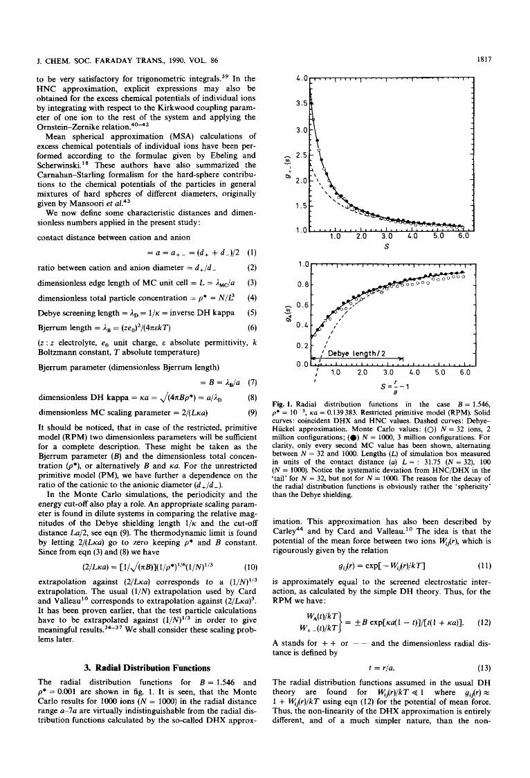
3. Radial Distribution Functions The radial distribution functions for B = 1.546 and p* = 0.001 are shown in fig. 1. It is seen, that the Monte Carlo results for lo00 ions (N = lo00) in the radial distance range a-7a are virtually indistinguishable from the radial dis- tribution functions calculated by the so-called DHX approx-
S
0 . 2 1 II 1
,' 1.0 2.0 3.0 4.0 5.0 6.0
a
I S J - ,
Fig. 1. Radial distribution functions in the case B = 1.546, p* = lop3, ~a = 0.139383. Restricted primitive model (RPM). Solid curves : coincident DHX and HNC values. Dashed curves : Debye- Hiickel approximation. Monte Carlo values: (0) N = 32 ions, 2 million configurations; (0) N = 1000, 3 million configurations. For clarity, only every second MC value has been shown, alternating between N = 32 and 1000. Lengths (L) of simulation box measured in units of the contact distance (a) L = : 31.75 ( N = 32), 100 (N = 1000). Notice the systematic deviation from HNC/DHX in the 'tail' for N = 32, but not for N = 1000. The reason for the decay of the radial distribution functions is obviously rather the 'sphericity' than the Debye shielding.
imation. This approximation has also been described by C a r l e ~ ~ ~ and by Card and Valleau." The idea is that the potential of the mean force between two ions &Ar), which is rigourously given by the relation
(1 1) gi,(r) = ~ X P C - Wjr)/k TI
is approximately equal to the screened electrostatic inter- action, as calculated by the simple DH theory. Thus, for the RPM we have :
A stands for + + or - - and the dimensionless radial dis- tance is defined by
t = r/a. (1 3) The radial distribution functions assumed in the usual DH theory are found for w,(r)/kT + 1 where gi,(r) w 1 + w,(r)/kT using eqn (12) for the potential of mean force. Thus, the non-linearity of the DHX approximation is entirely different, and of a much simpler nature, than the non-
1818
-1' Debye length120
J. CHEM. SOC. FARADAY TRANS., 1990, VOL. 86
linearity involved in solving the non-linear Poisson- Boltzmann equation. Notice the deficiencies of the DH approximation close to contact (dashed curves), especially the appearance of 'negative local concentrations' of ions with charges of the same sign as that of the central ion. Notice also, that the decay of the radial distribution functions towards unity is determined much more by the sphericity [the factor t in the denominator of eqn (12)] than by the Debye screening length.
The radial distribution functions calculated from the HNC approximation (8001 grid points in Fourier k-space, interval in ka = 0.025, maximum ka = 200) are also indistinguishable from the DHX distribution functions. The MC values for N = 32 (open circles in fig. 1) are identical to the DHX curves and to the MC values for N = lo00 (filled circles) close to contact, but for increasing radial distance a certain depres- sion of the distribution functions, especially gA(r), is noticed. For N = lo00 we have L/2 = 50 at the present ion concen- tration, whereas L/2 x 16 for N = 32. Apparently, a cut-off distance equal to 16 contact distances may be 'felt' slightly from r = 3a, whereas a cut-off distance equal to 50a has no influence even at r = 7a. In the former case the influence is felt from ca. 4 of the minimum image cut-off. In the latter case, the influence is not yet felt at f of the cut-off distance.
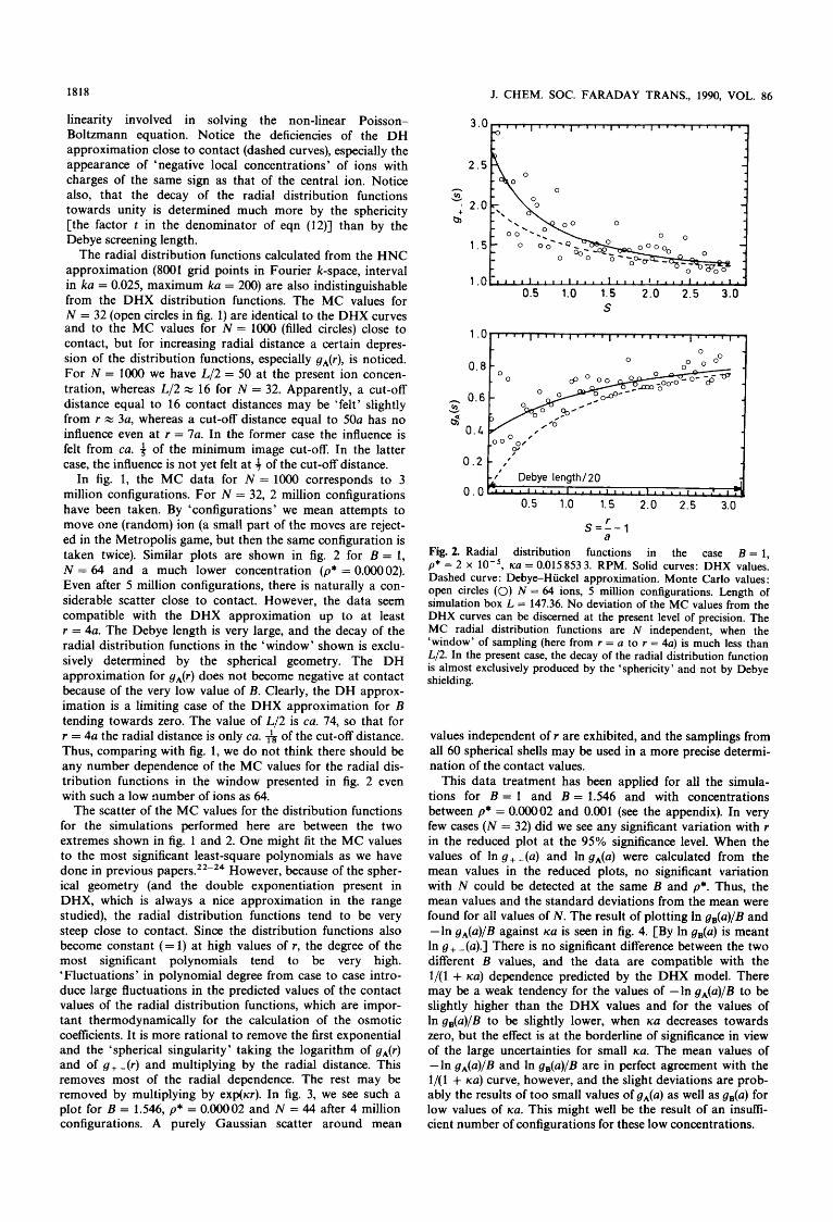
In fig. 1, the MC data for N = 10oO corresponds to 3 million configurations. For N = 32, 2 million configurations have been taken. By 'configurations' we mean attempts to move one (random) ion (a small part of the moves are reject- ed in the Metropolis game, but then the same configuration is taken twice). Similar plots are shown in fig. 2 for B = 1, N = 64 and a much lower concentration (p* = O.OOOO2). Even after 5 million configurations, there is naturally a con- siderable scatter close to contact. However, the data seem compatible with the DHX approximation up to at least r = 4a. The Debye length is very large, and the decay of the radial distribution functions in the 'window' shown is exclu- sively determined by the spherical geometry. The DH approximation for gA(r) does not become negative at contact because of the very low value of B. Clearly, the DH approx- imation is a limiting case of the DHX approximation for B tending towards zero. The value of L/2 is ca. 74, so that for r = 4a the radial distance is only ca. & of the cut-off distance. Thus, comparing with fig. 1, we do not think there should be any number dependence of the MC values for the radial dis- tribution functions in the window presented in fig. 2 even with such a low mmber of ions as 64.
The scatter of the MC values for the distribution functions for the simulations performed here are between the two extremes shown in fig. 1 and 2. One might fit the MC values to the most significant least-square polynomials as we have done in previous paper^.^^-^^ However, because of the spher- ical geometry (and the double exponentiation present in DHX, which is always a nice approximation in the range studied), the radial distribution functions tend to be very steep close to contact. Since the distribution functions also become constant (= 1) at high values of I , the degree of the most significant polynomials tend to be very high. 'Fluctuations' in polynomial degree from case to case intro- duce large fluctuations in the predicted values of the contact values of the radial distribution functions, which are impor- tant thermodynamically for the calculation of the osmotic coeflicients. It is more rational to remove the first exponential and the 'spherical singularity' taking the logarithm of gA(r) and of g+ - ( r ) and multiplying by the radial distance. This removes most of the radial dependence. The rest may be removed by multiplying by exp(ur). In fig. 3, we see such a plot for B = 1.546, p* = 0.00002 and N = 44 after 4 million configurations. A purely Gaussian scatter around mean
- - I l , , l I I , , , I .
0.5 1.0 1.5 2.0 2.5 3.0 S
ooVo,'
0 . 2 , 7
values independent of r are exhibited, and the samplings from all 60 spherical shells may be used in a more precise determi- nation of the contact values.
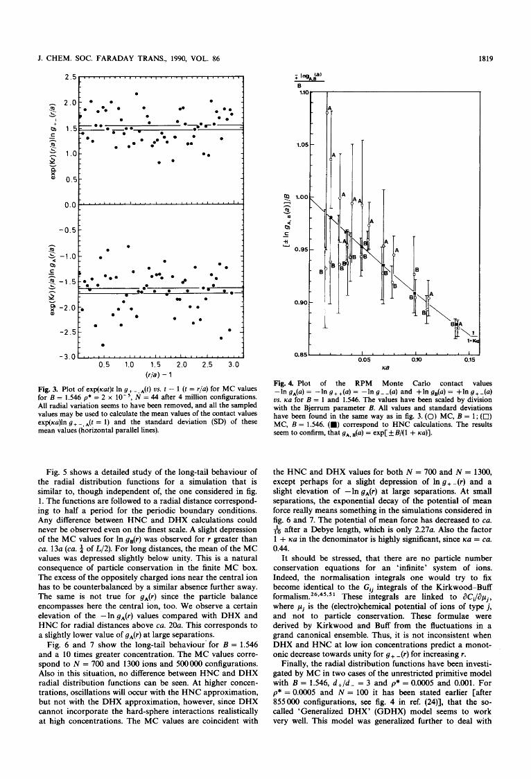
This data treatment has been applied for all the simula- tions for B = 1 and B = 1.546 and with concentrations between p* = 0.00002 and 0.001 (see the appendix). In very few cases (N = 32) did we see any significant variation with r in the reduced plot at the 95% significance level. When the values of In g + - (a) and In gA(a) were calculated from the mean values in the reduced plots, no significant variation with N could be detected at the same B and p*. Thus, the mean values and the standard deviations from the mean were found for all values of N. The result of plotting In gB(a)/B and -In gA(a)/B against KU is seen in fig. 4. [By In gB(a) is meant In g + -(a).] There is no significant difference between the two different B values, and the data are compatible with the 1/(1 + K U ) dependence predicted by the DHX model. There may be a weak tendency for the values of -In gA(a)/B to be slightly higher than the DHX values and for the values of In gB(a)/B to be slightly lower, when ua decreases towards zero, but the effect is at the borderline of significance in view of the large uncertainties for small K U . The mean values of -In g,(a)/B and In gB(a)/B are in perfect agreement with the 1/(1 + ua) curve, however, and the slight deviations are prob- ably the results of too small values of gA(a) as well as gB(a) for low values of UQ. This might well be the result of an insufi- cient number of configurations for these low concentrations.
J. CHEM. SOC. FARADAY TRANS., 1990, VOL. 86 1819
0 . -2.0r .- -2.51
.. . . . 0.5 1.0 1.5 2.0 2.5 3.0
( r b ) - 1
Fig. 3. Plot of exp(Kat)t In g+-.A(t) us. t - 1 (t = r/a) for MC values for B = 1.546 p* = 2 x N = 44 after 4 million configurations. All radial variation seems to have been removed, and all the sampled values may be used to calculate the mean values of the contact values exp(ica)ln g + -, *(t = 1) and the standard deviation (SD) of these mean values (horizontal parallel lines).
Fig. 5 shows a detailed study of the long-tail behaviour of the radial distribution functions for a simulation that is similar to, though independent of, the one considered in fig. 1. The functions are followed to a radial distance correspond- ing to half a period for the periodic boundary conditions. Any difference between HNC and DHX calculations could never be observed even on the finest scale. A slight depression of the MC values for In g,(r) was observed for r greater than ca. 13a (ca. $ of L/2). For long distances, the mean of the MC values was depressed slightly below unity. This is a natural consequence of particle conservation in the finite MC box. The excess of the oppositely charged ions near the central ion has to be counterbalanced by a similar absence further away. The same is not true for gA(r) since the particle balance encompasses here the central ion, too. We observe a certain elevation of the -In gA(r) values compared with DHX and HNC for radial distances above CQ. 2Oa. This corresponds to a slightly lower value of gA(r) at large separations.
Fig. 6 and 7 show the long-tail behaviour- for B = 1.546 and a 10 times greater concentration. The MC values corre- spond to N = 700 and 1300 ions and 500000 configurations. Also in this situation, no difference between HNC and DHX radial distribution functions can be seen. At higher concen- trations, oscillations will occur with the HNC approximation, but not with the DHX approximation, however, since DHX cannot incorporate the hard-sphere interactions realistically at high concentrations. The MC values are coincident with
B
0.05 030 0.15 Ka
Fig. 4. Plot of the RPM Monte Carlo contact values -In gA(a) = -In g++(a) = -In g--(a) and +In gB(u) = +In g+-(a) vs. rca for B = 1 and 1.546. The values have been scaled by division with the Bjerrum parameter B. All values and standard deviations have been found in the same way as in fig. 3. (0) MC, B = 1; (0) MC, B = 1.546. (m) correspond to HNC calculations. The results seem to confirm, that gA, = exp[ B/( 1 + KU)].
the HNC and DHX values for both N = 700 and N = 1300, except perhaps for a slight depression of In g+ -(r) and a slight elevation of -In gA(r) at large separations. At small separations, the exponential decay of the potential of mean force really means something in the simulations considered in fig. 6 and 7. The potential of mean force has decreased to CQ.
& after a Debye length, which is only 2 . 2 7 ~ . Also the factor 1 + KU in the denominator is highly significant, since ica = ca. 0.44.
It should be stressed, that there are no particle number conservation equations for an 'infinite' system of ions. Indeed, the normalisation integrals one would try to fix become identical to the Gij integrals of the Kirkwood-Buff formali~m.~ *4s*5 These integrals are linked to dC,/apj, where pj is the (e1ectro)chemical potential of ions of type j , and not to particle conservation. These formulae were derived by Kirkwood and Buff from the fluctuations in a grand canonical ensemble. Thus, it is not inconsistent when DHX and HNC at low ion concentrations predict a monot- onic decrease towards unity for g+ -(r) for increasing r.
Finally, the radial distribution functions have been investi- gated by MC in two cases of the unrestricted primitive model with B = 1.546, d + / d - = 3 and p* = O.OOO5 and 0.001. For p* = 0.0005 and N = 100 it has been stated earlier [after 855000 configurations, see fig. 4 in ref. (24)], that the so- called 'Generalized DHX' (GDHX) model seems to work very well. This model was generalized further to deal with

1820 J. CHEM. SOC. FARADAY TRANS., 1990, VOL. 86
2 .o h
v c I
G 1.0 C -
0.0
- o . o [ . . r . 1 , I I I I I I I 1 I I I 1 I I I , I I I ,
5 10 15 20 25 30 35 40 45 s = @/a) - 1
Fig. 5. Monte Carlo investigation of the long-tail behaviour of the potentials of mean force [WJr)/kT = -In g&)] for the RPM, B = 1.546, p* = N = 1000 after 2 million configurations. The simulation is independent of the one shown in fig. 1. (0) MC values; solid curves are calculated by the HNC or the DHX theories. These two approximations lead to indistinguishable results in the present case, even for the largest r values shown. It should be noticed, that the DHX expressions for the potential of mean force is equivalent to the expression for 'the electrostatic potential around a central ion' in the ordinary theory of Debye and Huckel. The distance of minimum image energy cut-off is L/2 = 50 (measured in units of a). The MC values deviate systematically from the HNC/DHX curves for s > CQ. 15. [s = @/a) - 13.
10
a h
A 6 dr s 4
+
2
0
5 15 20 25 10 s = @/a) - 1
Fig. 6. Monte Carlo investigation of the long-tail behaviour of the potential of mean force between dissimilar ions for the RPM, B = 1.546, p* = 0.01, KU = 0.440767 6, N = 700 (0) and N = 1300 (w) after 500000 configurations. The solid curves are calculated by the HNC and DHX theories, which are still indiscernible at the present concentration. Debye shielding is clearly competing with sphericity in determining the decay of the radial distribution functions towards unity. The distance of minimum image energy cut-off is L/2 = 20.6 for N = 700 and 25.3 for N = 1300 (measured in units of a).
5 10 15 20 25 s = (r/a) - 1
Fig. 7. Monte Carlo investigation of the long-tail behaviour of the potential of mean force between similar ions for the RPM, B = 1.546, p* = 0.01, KU = 0.440 767 6, N = 700 (0) and N = 1300 (D) after 500 000 configurations. The solid curves are calculated by the HNC and DHX theories, which yield coincident values. Same comments as for fig. 6.
J. CHEM. SOC. FARADAY TRANS., 1990, VOL. 86 1821
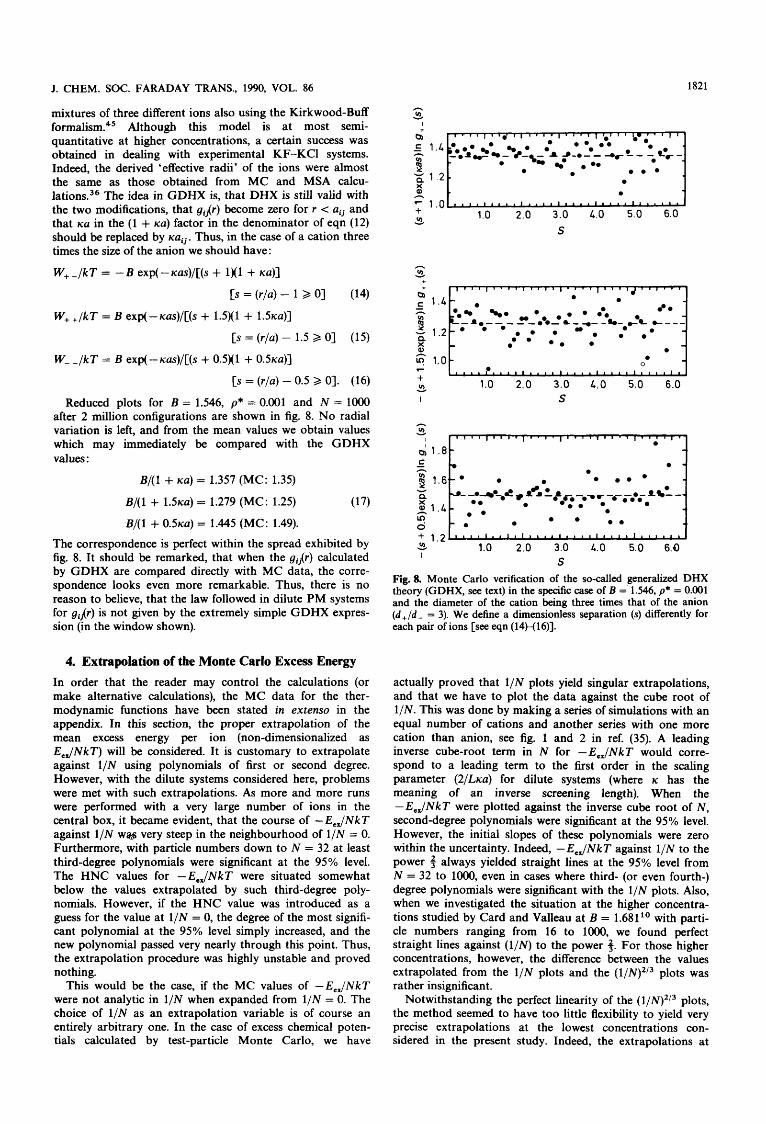
n mixtures of three different ions also using the Kirkwood-Buff Y f o r m a l i ~ m . ~ ~ Although this model is at most semi- quantitative at higher concentrations, a certain success was obtained in dealing with experimental KF-KCl systems. Indeed, the derived 'effective radii' of the ions were almost the same as those obtained from MC and MSA calcu- l a t i o n ~ . ~ ~ The idea in GDHX is, that DHX is still valid with the two modifications, that gij(r) become zero for r < uij and that KU in the (1 + KU) factor in the denominator of eqn (12) should be replaced by xuij. Thus, in the case of a cation three times the size of the anion we should have:
W+-/kT = - B exp(-icus)/[(s + 1x1 + KU)]
[S = ( r / ~ ) - 1 2 01 (14)
W+ +/kT = B exp(-Kus)/[(s + 1.5)(1 + 1.51cu)l
[S = ( r / ~ ) - 1.5 2 01 (15)
W- JkT = B exp(--m)/[(s + 0.5)(1 + OSKU)]
[S = (r/a) - 0.5 2 01. (16)
Reduced plots for B = 1.546, p* = 0.001 and N = lo00 after 2 million configurations are shown in fig. 8. No radial variation is left, and from the mean values we obtain values which may immediately be compared with the GDHX values:
B/(1 + KU) = 1.357 (MC: 1.35)
B/(1 + 1 . 5 ~ ~ ) = 1.279 (MC: 1.25) (17)
B/(1 + 0 . 5 ~ ~ ) = 1.445 (MC: 1.49).
The correspondence is perfect within the spread exhibited by fig. 8. It should be remarked, that when the g&) calculated by GDHX are compared directly with MC data, the corre- spondence looks even more remarkable. Thus, there is no reason to believe, that the law followed in dilute PM systems for g&) is not given by the extremely simple GDHX expres- sion (in the window shown).
4. Extrapolation of the Monte Carlo Excess Energy In order that the reader may control the calculations (or make alternative calculations), the MC data for the ther- modynamic functions have been stated in extenso in the appendix. In this section, the proper extrapolation of the mean excess energy per ion (non-dimensionalized as E,JNkT) will be considered. It is customary to extrapolate against 1/N using polynomials of first or second degree. However, with the dilute systems considered here, problems were met with such extrapolations. As more and more runs were performed with a very large number of ions in the central box, it became evident, that the course of -E,JNkT against 1/N w e very steep in the neighbourhood of 1/N = 0. Furthermore, with particle numbers down to N = 32 at least third-degree polynomials were significant at the 95% level. The HNC values for -E ,JNkT were situated somewhat below the values extrapolated by such third-degree poly- nomials. However, if the HNC value was introduced as a guess for the value at 1/N = 0, the degree of the most signifi- cant polynomial at the 95% level simply increased, and the new polynomial passed very nearly through this point. Thus, the extrapolation procedure was highly unstable and proved nothing.
This would be the case, if the MC values of -E ,JNkT were not analytic in 1/N when expanded from 1/N = 0. The choice of 1/N as an extrapolation variable is of course an entirely arbitrary one. In the case of excess chemical poten- tials calculated by test-particle Monte Carlo, we have
. ~ ~ ~ ~ ~ ~ ' " ~ ~ ~ ~ ~ ~ ' ' ' ' " ' ' ~ ~ ~ ~ ~ ' ~ ~
v) 1.0 2.0 3.0 4.0 5.0 6.0 W
S
h
3 *
F + 1.0 2.0 3.0 4.0 5.0 6.0 v, Y
I S
n r n
Y L2' ' \:o ' I ;Id ' ''ii ' ' '4:; ' I;.; I 'sf; ' S
Fig. 8. Monte Carlo verification of the so-called generalized DHX theory (GDHX, see text) in the specific case of B = 1.546, p* = 0.001 and the diameter of the cation being three times that of the anion ( d + / d - = 3). We define a dimensionless separation (s) differently for each pair of ions [see eqn (14H16)I.
actually proved that 1/N plots yield singular extrapolations, and that we have to plot the data against the cube root of 1/N. This was done by making a series of simulations with an equal number of cations and another series with one more cation than anion, see fig. 1 and 2 in ref. (35). A leading inverse cube-root term in N for -E,JNkT would corre- spond to a leading term to the first order in the scaling parameter (2/L~a) for dilute systems (where K has the meaning of an inverse screening length). When the -E,JNkT were plotted against the inverse cube root of N, second-degree polynomials were significant at the 95% level. However, the initial slopes of these polynomials were zero within the uncertainty. Indeed, -E,JNkT against 1/N to the power 4 always yielded straight lines at the 95% level from N = 32 to 1O00, even in cases where third- (or even fourth-) degree polynomials were significant with the 1/N plots. Also, when we investigated the situation at the higher concentra- tions studied by Card and Valleau at B = 1.681'' with parti- cle numbers ranging from 16 to 1O00, we found perfect straight lines against (l/N) to the power 4. For those higher concentrations, however, the difference between the values extrapolated from the 1/N plots and the (l/N)2/3 plots was rather insignificant.
Notwithstanding the perfect linearity of the ( l/N)2/3 plots, the method seemed to have too little flexibility to yield very precise extrapolations at the lowest concentrations con- sidered in the present study. Indeed, the extrapolations at

1822 J. CHEM. SOC. FARADAY TRANS., 1990, VOL. 86
0.1 0.2 0.3 0.4 ( 1 1 ~ ) 1/3
Fig. 9. Three plots of Eex(rel) = [E,,(MC)/NkT]/[E,,(extrapolated)/ NkT] us. (l/N)1/3 for the RPM. (a) B = 1.546, p* = 2 x lo-’; (b) B = 1.546, p* = (c) B = 1.681, p* = 0.009595. It seems plaus- ible that the first ‘size of the box’ term is of the order of # in (l/N).
very low concentrations now yielded values of -E,JNkT lower than the HNC values.
To make the polynomials more flexible, one might use third-degree polynomials in the inverse cube root of N enforcing an initial slope equal to zero. This has been done in three situations (fig. 9). The concentration increases from top to bottom. At the highest concentration (a Card-Valleau system), the Monte Carlo values indeed seem to be almost independent of the inverse cube root of N (apart from some noise) from 216 up to 1000 ions. (For the lowest concentra- tion, the curvilinear extrapolation has to be done over a con- siderable distance, making the estimate quite uncertain.)
In order to use the MC simulations in a more concerted manner, the following ‘calibration procedure’ was decided. Since we have seen in the previous section, that the DHX model is very good in dilute systems for the radial distribu- tion functions, we assume that the DHX values for E,JNkT (obtained by numerical integration from contact distance to at least 15 Debye screening lengthsz3) are also very represen- tative for the limiting MC values at the two lowest concentra- tions (p* = 0.00002 and 0.000064). The MC values were scaled relative to these values. With B = 1 and 1.546, we have in total 35 values. Next, these values were plotted against 2/(Lica). Indeed, a common ‘calibration curve’ could be pro- duced by a least-square fit with the constraints, that the curve should go through (0, 1) and should have an initial slope equal to zero, see fig. 10. In order to have good flexibility in the curve, a fourth-degree polynomial was used. The cali-
I l l l l l l l l l l l l l l l l l
2/(L-) 0.1 0.2 0.3 0.4 0.5 0.6 0.7 0.8
Fig. 10. Calibration polynomial for extrapolation of E,,(MC) values. For B = 1 and 1.546 and p* = 0.00002 and 0.000064, the values of E,,(MC)/E,,(DHX) for 35 individial Monte Carlo runs have been plotted against ( ~ / L K u ) . Solid curve: The polynomial given by eqn (18). MC points: (0) B = 1, p* = 2 x lo-’. (RPM): 0) B = 1.546, p* = 2 x lo-’; (V) B = 1, p* = 6.4 x lo-’; (V) B = 1.546, p* = 6.4 x 10⁻⁵.
bration polynomial is:
E,,(MC)/E,,( 00) = 1 + 0.1 52 526(2/Lic~)~
+ 0.783 5 5 5 ( 2 / L ~ ~ ) ~ - 0.452 61(2/Lic~)~. (18)
The fact that the four different series of simulations rescale to a common curve with E,,(oo) = E,,(DHX) makes it plausible, that E,,(DHX) is close to the thermodynamic limit (N = 00).
If the curve has to bend through the point (0, 1) it does indeed have to have a very small initial slope. We shall shortly obtain an u posteriori verification of the strong initial curvature of the calibration curve by the successful prediction for the other simulations.
In fig. 11, the simulations with B = 1, B = 1.546, p* = 0.000 125, 0.00025, 0.0005, 0.001 and a range of ion numbers from 32 to lo00 have been plotted in a ‘universal’ plot. The calibration polynomial (18) was used, and the Monte Carlo values of E,JNkT were for each (B, p*) divided by the value of E,,(co)/NkT which gave the minimum sum of squared deviation from the calibration curve. The fit to the shape of the curve is remarkable. Notice especially the range of ‘prediction’ from (2/Licu) equal to 0.14-0.25. The simula- tions from which the calibration curve was constructed all had (~/LKu) > 0.25. The suggestion concerning the very curved first part of the calibration curve is verified.
Dilute systems with unequal radii of the cations and the anions also seem to follow the polynomial (18). Fig. 12 shows the simulations for B = 1.546, p* = 0.0005, 0.001 and d + / d - = 3 on the universal plot. The extrapolated values Eex( oo)/NkT differ slightly, but significantly, between situ- ations with equal and unequal radii (with B and p* the same). In order to demonstrate how precisely the thermody- namic limit may be estimated in dilute systems even from simulations with a very small number of particles, we have

J. CHEM. SOC. FARADAY TRANS., 1990, VOL. 86 1823
r
0.1 0.2 0.3 0 . 4 0.5 0.6 2/ (L- )
Fig. 11. 'Universal' plot of E,,(MC)/E,,(oo) us. (~/LKu) for a number of individual Monte Carlo runs for B = 1 (open) and B = 1.546 (black) and p* = 0.000 125 (0, a), 0.00025 (a, a), 0.0005 (A, A) and 0.001 (0, m). For each concentration, the value ofE,,(co),/NkT has been obtained as the divisor resulting in the best least-squares fit to the calibration polynomial [fig. 10 and eqn (18)]. The following extrapolated values were obtained. B = 1, p* = 0.000 125, -E,,(oo)/NkT = 0.019 16; B = 1.546, p* = 0.000 125, -E, , (co) /NkT = 0.03679; B = 1, p* = 0.00025, - E e x ( ~ ) / N k T = 0.02683; B = 1.546, p* = 0.00025, - E , , ( a ) / N k T = 0.037 10; B = 1.546, p* = 0.0005, - E e , ( ~ ) / N k T = 0.07080; B = 1, p* = 0.001, - E e , ( ~ ) / N k T = 0.05102; B = 1.546, p* = 0.001, - E , , ( a ) / N k T = 0.09678.
- E , , ( w ) / N k T = 0.051 26; B = 1, p* = 0.0005,
(Uncertainties ca. f0.00005, see fig. 12 and table 1.) The 'prediction' interval exceeds the lower limit of (~ /LKu) for which Monte Carlo data were used in the construction of the calibration polynomial (fig. 10). The hypothesis, that the first 'size term' is of second order in (2/L~a) or of order 4 in (l/N) is supported.
compared in table 1 for B = 1.546 and p* = 0.0005 and 0.001 the original MC values at a given N with the values obtained from the calibration method using N values equal to and less than the N values in the entry. Although the MC values vary widely with N, there is no systematic variation in the esti- mates, and the estimate based on one single simulation for N = 32 (or 64) is very close to the final value (using all simulations).
We would not expect the 'universal' scaling to be valid at higher concentration, since IC loses its simple meaning as the
1.08
1.07
1.06 h
8 - 1.05
o 1.04
Q" 1.03
1 I I I I I I I I J 0.1 0.2 0.3 0.4
2/ (L- )
Fig. 12. The Monte Carlo simulations with a cation three times the size of the anion ( d + / d - = 3); B = 1.546 and p* = 0.0005, 0.001 also fit to the calibration polynomial (fig. 10) with the following extrapo- lated values: [ -E, , (oo)/NkT] x 100 = 7.098 & 0.005, p* = 0.0005 (a); [ -E, , (oo)/NkT] x 100 = 9.711 f 0.005, p* = 0.001 (m). The uncertainties are taken from table 1.
inverse screening length for the 'ionic cloud'. Fig. 13 shows an attempt to scale the MC values for B = 1.681 and p* = 0.009595. The data do not follow the calibration curve
Table 1. Treatment of Monte Carlo results for E J N k T for B = 1.546, p* = 0.0005 and 0.001 and d + / d - = 3
100 ( - E , , / N k T )
N" Monte Carlo N = 00, least-squaresb
64 80
100 150 216 3 50 512 700 03
32 44 50 64 70 80
100 120 150 180 216 3 50 512
1000 a3
KU = 0.098 558 6 7.561 7.475 7.391 7.339 7.298 7.205 7.175 7.147
KU = 0.139 383 10.54 10.33 10.26 10.19 10.14 10.1 1 10.04 9.994 9.933 9.919 9.907 9.832 9.775 9.788
p* = 0.0005 7.106 7.101 7.093 7.097 7.103 7.101 7.100 7.098
7.098 f 0.005
9.7 18 9.707 9.701 9.706 9.705 9.707 9.708 9.709 9.708 9.709 9.71 1 9.71 1 9.709 9.71 1
9.71 1 f 0.005
p* = 0.001
a For the column 'Monte Carlo', N is the number of ions in the simulations. For the second column, N is the maximum number of ions incorporated in the least-squares extrapolation to N = 00. Best fit of E,,(CO) to E,,(MC)/E,,(~) = 1 + 0.152 526(2/L~u)' + 0.783 555 ( ~ / L K u ) ~ - 0.452 61(2/L~u)~. This polynomial is based on a least- squares fit to 35 simulations for the RPM with B = 1 and 1.546, p* = 0.00002 and 0.000064 assuming E,,(m) = E,,(DHX) for these low concentrations.
1824
1 .o:
1.ot
1.Oi
1 .OE h v)
2 : 1.OE 5:
2 v 1.04
!!%
+ (0
X
O 1.03 5 Lu"
1.02
1.01
N=16
CC"W
I I I I 1 I 1 I I 0.1 0.2 0.3 0.1
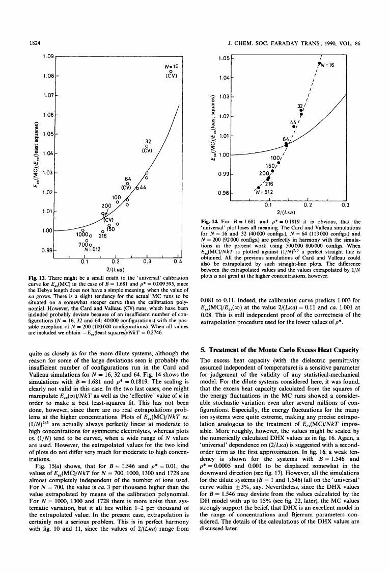
2 / ( L a ) Fig. 13. There might be a small misfit to the 'universal' calibration curve for E,,(MC) in the case of B = 1.681 and p* = 0.009595, since the Debye length does not have a simple meaning, when the value of KU grows. There is a slight tendency for the actual MC runs to be situated on a somewhat steeper curve than the calibration poly- nomial. However, the Card and Valleau (CV) runs, which have been included probably deviate because of an insufficient number of con- figurations (N = 16, 32 and 64: 40000 configurations) with the pos- sible exception of N = 200 (100000 configurations). When all values are included we obtain - E,,(least squares)/NkT = 0.2746.
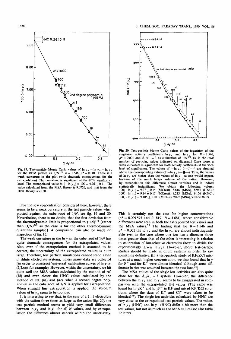
quite as closely as for the more dilute systems, although the reason for some of the large deviations seen is probably the insufficient number of configurations run in the Card and Valleau simulations for N = 16, 32 and 64. Fig. 14 shows the simulations with B = 1.681 and p* = 0.1819. The scaling is clearly not valid in this case. In the two last cases, one might manipulate E,,(oo)/NkT as well as the 'effective' value of K in order to make a best least-squares fit. This has not been done, however, since there are no real extrapolations prob- lems at the higher concentrations. Plots of E, , (MC)/NkT us. (l/N)2/3 are actually always perfectly linear at moderate to high concentrations for symmetric electrolytes, whereas plots us. (l/N) tend to be curved, when a wide range oi N values are used. However, the extrapolated values for the two kind of plots do not differ very much for moderate to high concen- trations.
Fig. 15(a) shows, that for B = 1.546 and p* = 0.01, the values of E,,(MC)/NkT for N = 700,1000, 1300 and 1728 are almost completely independent of the number of ions used. For N = 700, the value is ca. 3 per thousand higher than the value extrapolated by means of the calibration polynomial. For N = 1O00, 1300 and 1728 there is more noise than sys- tematic variation, but it all lies within 1-2 per thousand of the extrapolated value. In the present case, extrapolation is certainly not a serious problem. This is in perfect harmony with fig. 10 and 11, since the values of 2/(L~a) range from
J. CHEM. SOC. FARADAY TRANS., 1990, VOL. 86
1.04
' - O 5 I 1.03
2 3 0 : 1.02 Q - v X
g 1.01 s 5 Lu" 1.00
0.99
0.98
0.1 0.2 0.3 2/ (L- )
Fig. 14. For B = 1.681 and p* = 0.1819 it is obvious, that the 'universal' plot loses all meaning. The Card and Valleau simulations for N = 16 and 32 (40000 configs.), N = 64 (113000 configs.) and N = 200 (92000 configs.) are perfectly in harmony with the simula- tions in the present work using 500000-800000 configs. When E,,(MC)/NLT is plotted against (l/N)2/3 a perfect straight line is obtained. All the previous simulations of Card and Valleau could also be extrapolated by such straight-line plots. The difference between the extrapolated values and the values extrapolated by 1/N plots is not great at the higher concentrations, however.
0.081 to 0.11. Indeed, the calibration curve predicts 1.003 for E,,(MC)/E,,(oo) at the value 2/(L~a) = 0.11 and ca. 1.001 at 0.08. This is still independent proof of the correctness of the extrapolation procedure used for the lower values of p*.
5. Treatment of the Monte Carlo Excess Heat Capacity The excess heat capacity (with the dielectric permittivity assumed independent of temperature) is a sensitive parameter for judgement of the validity of any statistical-mechanical model. For the dilute systems considered here, it was found, that the excess heat capacity calculated from the squares of the energy fluctuations in the M C runs showed a consider- able stochastic variation even after several millions of con- figurations. Especially, the energy fluctuations for the many ion systems were quite extreme, making any precise extrapo- lation analogous to the treatment of E, , (MC)/NkT impos- sible. More roughly, however, the values might be scaled by the numerically calculated DHX values as in fig. 16. Again, a 'universal ' dependence on (2/Llca) is suggested with a second- order term as the first approximation. In fig. 16, a weak ten- dency is shown for the systems with B = 1.546 and p* = 0.0005 and 0.001 to be displaced somewhat in the downward direction (see fig. 17). However, all the simulations for the dilute systems (B = 1 and 1.546) fall on the 'universal' curve within &3%, say. Nevertheless, since the DHX values for B = 1.546 may deviate from the values calculated by the DH model with up to 15% (see fig. 22, later), the M C values strongly support the belief, that DHX is an excellent model in the range of concentrations and Bjerrum parameters con- sidered. The details of the calculations of the DHX values are discussed later.

J. CHEM. SOC. FARADAY TRANS., 1990, VOL. 86 1825
I I I I I I I 0
N= 700 / / 1.003 1
h
8 v s 1.002
1 .ooo t------
700 0
1000 0
I 1 I 1 I I 1
1 .oo
0.90
0.80
0.70
0.02 0.04 0.06 0.08 0.10 0.12
2/(LKa) Fig. 15. For B = 1.546 and p* = 0.01 (RPM), there is almost no variation in E,,(MC)/NkT (few per thousand) with the number of ions (N), when N passes from 700 through lo00 and 1300 towards 1728. (a) By means of the calibration curve, the extrapolated value E,,(m)/NkT is found to be -0.2464 f 0.0002 by least-squares. (b) The solid curve is 1 - 0.695x2, with x = ( 2 / L ~ a ) corresponding to the first straight part of the calibration curve for C,,, , (fig. 16 and 17). The extrapolated value is found to be C,,,,(oo)/Nk = 0.103 & 0.005 by least-squares. (c) In y ,(test) us. (2/Lica). A straight-line extrapo- lation is made to (2/Lica) = 0 (N = 00) [i - 2.35 (2/Lica)]. This extrapolation would be rather bold if done in isolation; but see fig. 19 and 20, where similar plots with many more N values show that the first size term is of the order of (2/Lica) to the first power. The extrapolated value is In y, = -0.213 & 0.008. The hard-sphere con- tribution is In y(H.S.) = + 0.042 30 (Carnahan-Starling and Percus- Yevick yield identical values). Thus, the electrostatic contribution is In y,(el test) = -0.255 & 0.008.
Already Card and Valleau" stated that the DHX values for the heat capacity were not incompatible with the MC cal- culations. However, they used very few configurations and ion numbers (and considerably higher concentrations) and any strong case cannot be made from their figures.
In fig. 17, the values of C,,,,(MC)/C,,,,(DHX) for B = 1.546 and p* = 0.0005 and 0.001 have been plotted against the square of (2/Llca) for d + / d - = 1 as well as 3. No significant difference can be seen between the simulations with equal radii and the simulations with the cation three times larger than the anion. However, all simulations seem to be situated ca. 2% below the common 'calibration curve' (a straight line in this range) taken from fig. 16. [We look apart
0.60 0 . 6 5 ~ 0.1 0.2 0.3 0.4 0.5 0.6 0.7 0.8
4/(LKaI2
Fig. 16. 'Universal' scaling of the RPM Monte Carlo excess heat capacity. The ratio Cv, ,,(MC)/C,, ,,(DHX) is plotted against ( 2 / L ~ a ) . ~ The fluctuations are quite formidable for large systems (small 2 / L ~ a ) . The points are individual MC runs with B = 1 and B = 1.546 at six different values of p*. The symbols are as in fig. 10 and 11. The DHX-values are confirmed within a few percent. The solid curve is given by 1 - 0 . 6 9 5 ~ ~ + 0.28xs, x = (2/Lica).
from some noisy values for high N, i.e. low 2/(L~a).] The best which can be done is simply to say that the N = co values for those four series of simulations are ca. 2% lower than calcu- lated by the DHX model.
6. Treatment of the Salsburflhesnut Values for AFJNk T
The electrostatic contribution to the excess Helmholtz free energy may be calculated from the DHX model as well as from the HNC formalism (see section 8). When the Salsburg- Chesnut MC values were scaled by the DHX values and plotted against 2 / (L~a) , a 'universal' plot was produced for B = 1 and 1.546 and p* = 0.00002 and 0.000064 (fig. 18). Thus, we may tentatively use a 'calibration polynomial' with the same form as for E,, in order to extrapolate the values to N = 0 :
AF,,(MC)/AF,,(CO) = 1 + 1.067 34 ( 2 / L ~ a ) ~
+ 0.729 190 ( ~ / L K u ) ~ - 0.840 83 ( ~ / L K u ) ~ . (19)
Fig. 18 exhibits considerable scatter in the values for low values of 2/(L~a) (large values of N). At concentrations of p* = 0.000 125 and above, an increasing tendency is seen for the -AF,,(MC)NkT values not only to scatter at high N values, but also to be of a too high value. The reason is, that in the Salsburg-Chesnut method, the exponential function of the dimensionless configurational energy U,JkT is sampled in a Metropolis Markov process optimized to sample mostly for small values of U,JkT. However, it is the most unlikely

1826 J. CHEM. SOC. FARADAY TRANS., 1990, VOL. 86
Table 2. Treatment of Salsburg-Chesnut values for AF,,/NkT ; B = 1; RPM
100 (-AF,,/NkT) ~
N" Monte Carlo N = co, least-squaresb
64 100 150 216 350 512 700
1000 co
64 100 150 216 3 50 512 700
1000 00
32 44 64
100 150 216 350 512 700
1000 00
36 44 54 80
150 216 3 50 430 512 00
KU = 0.039 633 3 1.904 1.752 1.654 1.570 1.507 1.438 1.460 1.298
KU = 0.056 049 9 2.506 2.338 2.222 2.171 2.040 2.017
(2.047) (2.012)
KU = 0.079 266 5 3.717 3.503 3.294 3.100
2.97613.006 2.909 2.826 2.69 1
(2.78 1) (2.820/2.8 15)
KU = 0.1120998 4.757 4.577 4.449 4.232 3.99 1 3.941
(3.9 17) (3.744) (3.690)
p* = 0.000 125 1.291 1.290 1.291 1.292 1.293 1.292 1.296 1.288
1.292 f 0.004
1.812 1.814 1.817 1.825 1.823 1.826
(1.835) (1.841)
1,820 f 0.010
p* = 0.00025
p* = 0.0005 2.521 2.521 2.52 1 2.522 2.529 2.533 2.537 2.534
(2.541) (2.561)
2.525 0.010
p* = 0.001 3.51 1 3.500 3.499 3.498 3.500 3.508
(3.523) (3.522) (3.519)
3.500 i- 0.010
For the column 'Monte Carlo', N is the number of ions in the simulations. For the second column, N is the maximum number of ions incorporated in the least-squares extrapolation to N = co. Best fit of AF,,(m) to AF,,(MC)/AF,,(~) = 1 + 1.06734 (~/LKu)' + 0.729 190 ( ~ / L K u ) ~ - 0.84083 ( ~ / L K u ) ~ . This polynomial is based on a least-squares fit to 35 simulations for the RPM with B = 1 and 1.546, p* = 0.000 02 and O.OO0 064, assuming AFex( 00) = AF,,(DHX) for these low concentrations. Extrapolation values in parenthesis in the second column have been omitted (high N, p* and B). These values show systematic deviations (too high absolute values) and/or extreme fluctuations.
" For the column 'Monte Carlo', N is the number of ions in the simulations. For the second column, N is the maximum number of ions incorporated in the least-squares extrapolation to N = m.
Best fit of AF,,(oo) to AF,,(MC)/AF,,(oo) = 1 + 1.06734 (2/ LKU)' + 0.729 190 ( ~ / L K u ) ~ - 0.840083 ( ~ / L K u ) ~ . This polynomial is based on a least-squares fit to 35 simulations for the RPM with B = 1 and 1.546, p* = 0.00002 and 0.0oO064 assuming AFex(m) = AF,,(DHX) for these low concentrations. Extrapolation values in parenthesis in the second column have been omitted (high N, p* and B). These values show systematic deviations (too high absolute values) and/or extreme fluctuations.
Table 3. Treatment of Salsburg-Chesnut values for AF,,/NkT; B = 1.546; d+/d- = 1 and 3
100 (-AF,,/NkT)
N" Monte Carlo N = 00, least-squaresb
32 44 64
100 150 216 512 700 00
32 44 64
100 150 216 512 700 00
32 34 36 44 50 64 68 80
100 216 512
lo00 00
64 80
100 150 216 3 50 512 700 00
32 44 64
100 150 216 3 50 512 700
lo00 a2
32 44 50 64 70 80
100 120 150 180 216 350 512
1000 co
KU = 0.0492793 p* = 0.000 125 3.680 3.468 3.222 3.069 2.962 2.807 2.708
(2.783)
KU = 0.069691 5 p* = 0.00025 4.832 4.577 4.318 4.139 3.995 3.855
(3.796) (3.875)
KU = 0.0985586 6.312/6.288
6.275 6.21 1
6.01 2/6.025 5.903 5.845 5.784 5.647 5.342
(5.445) (5.278/5.051)
(5.687)
p* = 0.0005
KU = 0.098 558 6 5.784 5.68 1 5.514 5.427 5.007 5.358
(5.23 8) (5.380)
p* = 0.0005
KU = 0.139383 8.271 7.989 7.654 7.444 7.214
(7.237) (7.267) (7.198) (7.614)
(7.734/7.321)
p* = 0.001
KU = 0.139383 p* = 0.001 8.343 7.940 7.904 7.752 7.670 7.513 7.533 7.448 7.390 6.986
(7.493) (7.221) (7.228) (7.977)
d,/d- = 1 2.476 2.477 2.470 2.473 2.480 2.478 2.48 1
(2.495) 2.478 f 0.008 d+/d- = 1
3.470 3.469 3.464 3.470 3.475 3.474
(3.487) (3.508)
3.470 f 0.010 d+/d- = 1
4.794 4.802 4.798 4.802 4.799 4.799 4.813 4.814 4.802
(4.816) (4.829) (4.868)
4.800 k 0.015 d+/d- = 3
4.826 4.839 4.829 4.842 4.801 4.839
(4.859) (4.896)
4.840 f 0.015 d+ld- = 1
6.6 15 6.629 6.625 6.635 6.635
(6.655) (6.690) (6.7 1 7) (6.787) (6.83 3)
6.625 f 0.015 d+/d- = 3
6.673 6.640 6.648 6.660 6.664 6.658 6.670 6.680 6.69 1 6.673
(6.704) (6.7 15) (6.732) (6.810)
6.670 f 0.020

J. CHEM. SOC. FARADAY TRANS., 1990, VOL. 86 1827
t D
0.80 1 I I l ' " l l l ' l ' l ' ' l l ' l I 1 1 ' 1
0.05 0.10 0.15 0.20
4/(L=3I2
Fig. 17. Plot of C", ,,(MC)/C,,,,(DHX) us. (2/L~a)' for B = 1.546 and p* =0.0o05 [ d + / d - = 1 (a); d + / d - = 3 (O)] and p* =0.001 [ d + / d - = 1 (m); d + / d - = 3 (a)]. Statistically, there seems to be no difference between any of the four cases. The mean curve is the first (linear) part of the curve in fig. 16 based on all six concentrations at the two Bjerrum parameters. It seems plausible, that the values of C", , , (co)/Nk for the four selected systems are ca. 2% below the values predicted by the DHX approximation.
configurations with very high configurational energies, which almost exclusively contribute to exp( U,JkT) . Since the elec- trostatic contribution to Helmholtz' free energy - AF,JNkT is given as minus the natural logarithm of the Metropolis mean of exp(U,JkT),22 the values will tend to be too high if one does not average over an excessive number of configu- rations, except for the lowest values of N and/or B and p*. Indeed, the values of -AF,JNkT were found earlier to be CQ. 5% above the DHLL values for the dimensionless concentra- tions 0.000064,0.000 125 and 0.00025 [ref. (22), fig. 6; ref. (23) fig. 5(b)], when simple extrapolations against 1/N were used.
In the present study, another method will be used for the extrapolation. The calibration polynomial (19) is used in con- nection with the Salsburg-Chesnut samplings for B = 1 and 1.546 and p* = O.OO0 125, 0.00025, 0.0005 and 0.001. The values of AF, , (m) with the least sum of squared deviations are used taking more and more N values into account (starting with the lowest numbers of ions). Table 2 and 3 show the numbers obtained. It is seen, that more and more of the higher N values have to be discarded all together with increasing p*, since their inclusion leads to too high values of -AF,JNkT. Inspection of the numbers in tables 2 and 3 give a certain idea of the extrapolated values of -AF,JNkT and the uncertainty in their determination. The method is far from perfect, but it is the best which can be done. Anyway, the Salsburg-Chesnut method will only work for the very
1
1
1
2 2 '
GI 5
I
$
61
1
1
1
0.1 0.2 0.3 0.4 0.5 0.6 0.7 0.8 2/ (L- )
Fig. 18. Calibration polynomial for the Monte Carlo excess Helm- holtz free energy. Constructed in the same way as the calibration polynomial for E,,(MC) (fig. lo), but the relative variation is much larger. There are considerable fluctuations for small values of (2/L~a) (large systems). Symbols for the individual Monte Carlo/Salsburg- Chesnut samplings: (0) B = 1, p* = 2 x (+) B = 1.546, p* = 2 x 10⁻⁵; (v) B = 1, p* = 6.4 x 10⁻⁵; (v) B = 1.546, p* = 6.4 x 10⁻⁵.
lowest B and/or p* values. However, the sampling of the Salsburg-Chesnut values together with E,JNkT and C , , J N k almost does not add to computing time. Further- more, a considerable 'overkill' of configurations have been used in order to get useful values of C,,, , /Nk and of the radial distribution close to contact in those dilute systems.
Using the procedure described, values of - AFex( m) /Nk T were obtained lying between the values calculated by the DH law and the DHLL law (see fig. 23, later). Thus, the devi- ations to the 'wrong' side of DHLL reported earlier seem to be an artefact produced by improper extrapolation against 1/N and inclusion of simulations with too high N values and too low numbers of configurations.
7. Treatment of Test Particle Single-ion Excess Chemical Potentials
Single-ion excess chemical potentials have been calculated for the two series with B = 1.546 and p* = 0.001 (equal and unequal ionic radii) by the test-particle r n e t h ~ d . ~ ~ J ~ In pre- vious simulations (at higher concentrations), it was demon- strated, that straight-line extrapolations of pex, , /kT = In yi us. the cube root of 1/N were very satisfactory for two-ion as well as three-ion The agreement was excellent for univalent ions, when the extrapolated test particle values were compared to mean ionic and/or single ionic activities obtained by other methods (MSA,18 Gibbs-Duhem integra- tion of osmotic coefficients from HNC,14 multistage sampling46 and optimized mode e ~ p a n s i o n ~ ~ ) .
1828 J. CHEM. SOC. FARADAY TRANS., 1990, VOL. 86
0.1 0.2 0.3 (1 /N) 1'3
Fig. 19. Test-particle Monte Carlo values of In y + = In y - = In y , for the RPM plotted vs. l/N1'3. B = 1.546, p* = 0.001. There is a weak curvature in the plot (with dramatic consequences for the extrapolation). The curvature is significant at the 95% significance level. The extrapolated value is (-ln y + ) x 100 = 9.26 +_ 0.11. The value calculated from the MSA theory is 9.0726, and that from the HNC theory is 9.150.
For the low concentration considered here, however, there seems to be a weak curvature in the test particle values when plotted against the cube root of 1/N, see fig. 19 and 20. Nevertheless, there is no doubt, that the first deviation from the thermodynamic limit is proportional to (l/N)1'3 [rather than (l/N)2/3 as the case is for the other thermodynamic quantities sampled]. A comparison can also be made on inspection of fig. 15.
The weak curvature in the In y 0s. the cube root of 1/N has quite dramatic consequences for the extrapolated values. Also, even if the extrapolation method is assumed to be correct, the uncertainty of the extrapolated values is quite large. Therefore, test particle simulations cannot stand alone in dilute electrolyte systems, unless many data are collected [in order to construct 'universal' calibration curves of In y us. (2/Llca), for example). However, within the uncertainty, we hit quite well the MSA values calculated by the method of ref. (18) and even closer the HNC values calculated by the method of ref. (41) and (42), when a second degree poly- nomial in the cube root of 1/N is applied for extrapolation. When straight line extrapolation is applied, the absolute values of In y, seem to be too low.
It is interesting to see that, in the case of a 1 : 1 electrolyte with the cation three times as large as the anion (fig. 20), the test particle method seems to yield very small differences between In y, and In y - for all N values, and by extrapo- lation the difference almost cancels within the uncertainty.
n b degree polynomial (9%)
Fig. 20. Test-particle Monte Carlo values of the logarithm of the single-ion activity coefficients In y + and In y - for B = 1.546, p* = 0.001 and d + / d - = 3 as a function of l/N'l3. (N is the total number of particles, values indicated on diagram.) Once more, a weak curvature is significant for both activity coefficients at the 95% level of significance. The values of -In y - (--0--) are situated above the corresponding values of -In y+ (-0-). Thus, the values of In y + are higher than the values of In y - as one would expect, because of the much larger volume of the cation. However, by extrapolation this difference almost vanishes and is indeed statistically insignificant. We obtain the following values : 100(-ln y + ) = 9.07 & 0.14 (MCtest), 8.816 (MSA), 8.967 (HNC); 100(-ln y - ) = 9.14 f 0.17 (MCtest), 9.233 (MSA), 9.176 (HNC); 100(-ln y + ) = 9.105 & 0.087 (MCtest), 9.025 (MSA), 9.072 (HNC).
This is certainly not the case for higher concentrations (p* = 0.009595 and 0.1819; B = 1.681), where considerable differences were seen in both the extrapolated test values and the MSA values3' The finding that for B = 1.546 and p* = 0.001 the In y + and the In y - are almost indistinguish- able even in the case where one ion has a diameter three times greater than that of the other is interesting in relation to calibration of ion-selective electrodes (how to divide the experimentally given In y *). However, more test-particle studies should be made in dilute systems in order to say something definitive. (In a test-particle study of KF/KCl mix- tures at a much higher concentration, we also found that In y for F - and for K+ were almost identical although some dif- ference in size was assumed between the two ions.36)
The MSA values of the single-ion activities are also quite close for the d + / d - = 3 system. However, the difference between the In y + and In y - seems to be exaggerated in com- parison with the extrapolated test values. (The same was found for In yK+ and In yF- in K F and mixed KF/KCl solu- tions, where the sizes of K + and C1- were taken to be iden t i~a l~~) . The single-ion activities calculated by HNC are very close to the extrapolated test-particle values. The values of In y, (HNC) and In y - (HNC) differ a bit more than the test values, but not as much as the MSA values (see also table 12 later).

J. CHEM. SOC. FARADAY TRANS., 1990, VOL. 86 1829
8. DHX and HNC Calculations and Consistency Checks
In section 3 it was found, that the DHX theory (the GDHX theory in the case of unequal ionic radii) was able to deliver radial distribution functions that were indistinguishable from Monte Carlo and HNC values, for distances from contact to quite far out in the ‘tails’ of the distribution functions. However, very far from contact, the comparison between DHX and MC or HNC is swamped by noise, since the devi- ations from unity are minute. Nevertheless, very small differ- ences far away from the ions may be of importance in very dilute systems.
For these reasons, a sensitive consistency check of the DHX theory for the RPM has been performed, calculating the electric contribution to the In y , in five different ways (tables 6 and 7). However, we shall first discuss the calcu- lation of E J N k T , AFJNkT and C,,,JNk from the DHX theory (tables 4 and 5). The value of the excess energy for the RPM can be directly evaluated by numerical integration of the difference between the first moments of the radial dis- tribution functions [see for example ref. (lo), eqn (S)] :
E,JNkT = [(Ka)2/4] lm[gA(t) - g+ -(t)]t dt (t = T/U). (20)
(It should be emphasised that, here and in the following, we mean by ‘moments’ the moments of the distributions with respect to the radial separation in the mathematical sense of the word. The word ‘moment’ in statistical mechanical liter- ature is often used somewhat differently, since the square of T
in 4nr2 is not counted). The expressions (11) and (12) were used, and the integrals were found by means of Gaussian q ~ a d r a t u r e . ~ ~ Weight factors for six points in each interval of a quarter of a Debye length were used and the integration was extended to 50 Debye lengths. Earlier, it was found that significant errors arise if the cut-off is less than ca. 8 Debye lengths [ref. (23) fig. 81. The digits stated in tables 4 and 5 are exact. Indeed, taking instead four or five Gaussian points in each interval of one-quarter of a Debye length or taking a somewhat shorter cut-off produces more coinciding digits than listed in the tables.
Apart from the calculations for B = 1 and 1.546, series of calculations were made of E,,(DHX)/NkT with B = 0.2, 0.4, 0.6, . .., 2.2 for each of the nine concentrations p* = O.OOOO2,
O.OOOO64, 0.OOO 125, 0.00025, 0.0005, 0.001, 0.003, 0.007 and 0.01. When the DHX value is scaled by the usual DH value
E,JNkT = ( - B/2)(ica)/( 1 + ica) (21)
[which may be obtained by expansion of the exponential of eqn (11) to the first two terms, using eqn (12)], it was observed that E,,(DHX)/E,,(DH) could be represented by a third-degree polynomial in B without the first-order term :
E,,(DHX)/E,,(DH) = 1 + a,B2 + BIB3. (22)
It should be stressed that there is a very strong dependence on B for B greater than ca. 2, so more terms have to be taken into account if B = 2.2 is exceeded. Afterwards, the coefi- cients a1 and B1 were fitted by a third-degree and a fifth- degree polynomial in ,/p*, respectively. These polynomials commence with the first-order term in p = ,/p* :
a1 = 0.312016~ - 2 . 6 1 3 5 ~ ~ + 7 . 9 0 0 9 4 ~ ~ (23)
B1 = 0.244 130p - 1 0 . 0 3 9 ~ ~ + 1 8 0 . 7 5 1 ~ ~
- 1 5 8 2 . 6 ~ ~ + 5335.67~’. (24)
The procedure might seem a bit obscure, but the column with label ‘polynomial’ in tables 4 and 5 shows indeed, that the overall approximation is very good. However, the approx- imation should not be used above B = 2.2 and above
The DHX heat capacity has been evaluated in two ways. Firstly, C,,, ,JNk may be evaluated by differentiation with respect to B under the integral sign. The final result for RPM is given as :
p* = 0.01.
c , ,JNk = (B/~XK~)’[CA + c+ -1 (25)
c.4 = c g A, DHX(s)exd - KaS)
1 + (K42) - (Icas/2) - ( [ K U ] s/ ’) ) ds (26) .( (1 + K u ) 2
g+ -,DHX(s)exd-Kas)
1 + (KU/2) - ( 4 2 ) - ([lcaI2s/2) (1 + K u ) 2
Table 4. DHX values compared to the Debye-Hiickel values for B = 1 and d + / d - = 1
2 x 10⁻⁵ 6.4 x 1 0 - 5
1.25 x 10⁻⁴ 2.5 x 10⁻⁴
5 x 10⁻⁴ 1 x 10⁻³ 3 x 10⁻³ 7 x 10⁻³ 1 x
1.58533 x 2.83593 x 3.96333 x lop2 5.60499 x 7.92666 x
1.120998 x lo-’ 1.941 626 x lo-’ 2.965883 x lo-’ 3.544908 x lo-’
1.002 20 1.003 70 1.004 82 1.00621 1.007 77 1.009 42 1.01 1 74 1.012 72 1.012 79
1.002 25 1.003 73 1.00488 1.00628 1.007 85 1.009 49 1.01 1 89 1.012 78 1.012 84
1.0131 1.0222 1.0290 1.0374 1 .O470 1.0573 1.0728 1.0810 1.0827
1.0132 1.0219 1.0287 1.0370 1.0463 1.0561 1.0719 1.0799 1.0820
1.OOO 859 1.001 459 1.001 914 1.002 485 1.003 139 1 .003 839 1.004846 1.005 280 1.005 313
1.OOO 876 1.001 460 1.001 918 1.002 487 1.003 135 1.003 824 1.004 858 1.005 269 1.005 310
~ ~~~
a Integration by means of six-point Gaussian quadrature in each quarter of a Debye length up to 50 Debye lengths. The DH law is E,,(DH)/NkT = -(B/~)(Ku)/(~ + KU). a, = 0.312016~ - 2 . 6 1 3 5 ~ ~ + 7 . 9 0 0 9 4 ~ ~ ; B1 = 0.244 130p - 1 0 . 0 3 9 ~ ~ + 180 .751~~ - 1 5 8 2 . 6 ~ ~ + 5335 .67~~ within the limits: B < 2.2; p* < 0.01. Differentiation with respect to B under the integral sign in the
DHX expression for E,, . The DH law is Cu, ,,/Nk = +(B/~)(Ku)/(~ + KU)’. 1 + a,(5 + 4~u)B’ + B,(7 + 6xu)B3, differentiation of the poly- nomial expression stated in footnote b with respect to B. Remember the variation of E,,(DH). By means of Gibbs-Helmholtz integration of the polynomial approximation for E,,(DHX). A third-degree polynomial in B of the form shown under b has been fitted for E,,(DHX)/E,,(DH) for each fixed value of p* in order to increase the precision relative to the expression stated under note b. The Gibbs-Helmholtz integration is performed from B = 0 using six-point Gaussian quadrature in B-intervals of size 0.002. The DH expression is AFex(DH)/NkT = -[B/(~u)*]Pn(l + KU) - KU + (KU)’/~]. ’ 1 + a2B2 + B 2 B 3 ; p = Jp*. a2 = 0.133995~ - 1 . 1 5 2 1 ~ ~ + 3 . 5 3 0 7 5 ~ ~ ; B2 = 0.081 1430p - 3 . 4 1 0 9 ~ ~ + 6 1 . 8 7 7 4 ~ ~ - 5 4 2 . 9 6 ~ ~ + 1831.45~’ within the limits: B < 2.2; p* < 0.01.
1 + a,B2 + B1B3; p = Jp*.

1830 J. CHEM. SOC. FARADAY TRANS., 1990, VOL. 86
P*
2 x 10-5 6.4 x 10⁻⁵ 1.25 x 10⁻⁴ 2.5 x 10⁻⁴ 5 x 10⁻⁴ 1 x 10⁻³ 3 x 10⁻³ 7 x 10⁻³ 1 x lo-’
Table 5. DHX values compared with the Debye-Huckel values for B = 1.546 and d + / d - = 1
E,,(DHX)/E,,(DH) C”, ,X(DHX)/C“, ,,(DH) A~,,(DHX)/AF,,(DH)
KU exact’ polynomialb exact‘ polynomiald exacte polynomialf
1.971 17 x lo-’ 1.006 58 1.006 56 1.040 1 1.0402 1.002 47 1.002 49 3.52614 x lo-’ 1.010 80 1.01074 1.066 1 1.0659 1.00409 1.00409
1.005 31 4.92793 x lo-’ 1.01390 1.013 88 1.0852 1.0853 1.005 30 1.006 78 6.96915 x lo-’ 1.017 59 1.017 59 1.1082 1.1084 1.006 76
9.85586 x lo-’ 1.021 59 1.021 50 1.1334 1.1330 1.008 38 1.008 37 1.009 96 1.393830 x lo-’ 1.025 52 1.025 26 1.1589 1.1571 1.01001 1.012 13 2.414184 x lo-’ 1.030 2 1 1.030 17 1.1926 1.1923 1.01209
3.687726 x lo-’ 1.031 11 1.030 98 1.2048 1.2040 1.012 68 1.012 67 4.407676 x lo-’ 1.030 55 1.030 52 1.2049 1.2050 1.012 55 1.012 56
As for table 4.
These integrals were evaluated numerically at the same time as the integrals for E,JNkT. In tables 4 and 5, the column under C,, ,,(DHX)/C,, ,,(DH) headed ‘exact’ is calculated that way, whereas the column headed ‘polynomial’ is calculated by differentiation of the polynomial (22) with respect to B:
+ b1(7 + 6ica)B3. (28)
[Remember that E,,(DH) is a function of rca, which is a func- tion of B ] . Again, the correspondence between the two columns is very good.
The last two columns in table 4 and 5 with the headings ‘Gibbs-Helmholtz’ and ‘polynomial’ are calculated as follows. The first by Gibbs-Helmholtz integration of the polynomial expression (22) from B = 0 (infinite temperature or zero charge) to B = 1 (table 4) or to B = 1.546 (table 5). In order to increase the precision, the expressions (23) and (24) have not been used. Instead, the two non-fixed polynomial coefficients in the third-degree polynomial were taken as the values found for each of the fixed values of p* (when B was varied from 0.2 to 2.2). The last column (‘polynomial’) is a polynomial approximation, analogous in form to eqn (22), for the AF,JNkT values obtained by the previous Gibbs- Helmholtz integration. This approximation is given by :
AF,,(DHX)/AF,,(DH) = 1 + a2 B2 + b2 B3 (29)
(30) a2 = 0.133 995p - 1 . 1 5 2 1 ~ ~ + 3.530 7 5 p 3
8 2 = 0.081 1 4 3 0 ~ - 3 . 4 1 0 9 ~ ~ + 61 .8774~~
- 5 4 2 . 9 6 ~ ~ + 1831.45~’ (31)
(P = JP*).
Inside its range of application (p* = 04.01, B = 0-2.2), the approximation (29)-(31) is seen to be very good by compari- son with the last two columns in tables 4 and 5.
It should be stressed that the AF,,/NkT calculated by the Gibbs-Helmholtz formula is not incorporating the hard- sphere contribution, which survives at infinite temperature or zero charge (B = 0) as the structural negentropy of the hard- sphere ordering. Thus, this hard-sphere free energy has to be added to the values in tables 4 and 5 to have the total values of the Helmholtz free energy. The values of E,JNkT are always purely electrostatic, of course.
In tables 6 and 7, the electrostatic contribution to the logarithm of the mean ionic activity coefficients In y , (at the given osmotic pressure according to the McMillan-Mayer approximation) have been calculated in five different ways as a very sensitive control of the thermodynamic consistency of the DHX model.
The columns headed ‘AF’ have been found by differentia- tion of the expressions (29)-(3 l) for AF(DHX)/AF(DH) with respect to p* (at constant volume and constant B). Since AF,, is only the electrostatic part of the excess Helmholtz free energy, we hereby also obtain the electrostatic part of the mean ionic excess chemical potential.
Table 6. Five different ways of calculating In y,(el, DHX) with B = 1 and d + / d - = 1
Kirkwood-Buff
P* K a AFa osmoticb inversion‘ g+ -(DHX)d gA(DHX)e mean KB
2 x 10⁻⁵ 6.4 x 10⁻⁵ 1.25 x 10⁻⁴ 2.5 x 10⁻⁴ 5 x 10⁻⁴ 1 x 10⁻³ 3 x 10⁻³ 7 x 10⁻³ 1 x lo-’
1.58533 x lo-’ 2.83593 x lo-’ 3.96333 x lo-’ 5.60499 x lo-’ 7.92666 x lo-’ 1.120998 x lo-’ 1.941 626 x lo-’ 2.965 883 x lo-’ 3.544908 x lo-’
1.001 14 1.001 87 1.002 43 1.003 08 1.003 80 1.00451 1.005 42 1.005 33 1.005 62
1.001 12 1.001 90 1.002 55 1.003 40 1.004 50 1.005 96 1.009 72 1.015 39 1.01941
1.001 81 1.003 41 1.00490 1.007 17 1.010 64 1.057 71 1.11035 1.115 24 1.12663
1.01491 1.022 12 1.027 16 1.033 02 1.039 44 1.08791 1.135 78 1.12501 1.124 19
0.983 37 0.975 07 0.969 06 0.961 89 0.953 89 0.987 01 1.010 33 0.982 11 0.974 59
1.OOO f 0.016 1.OOO f 0.024 1.OOO f 0.029 1.001 0.036 1.001 f 0.043 1.044 f 0.052 1.085 f 0.066 1.074 & 0.080 1.075 f 0.087
In y,(el, DH) = (-B/~)(Ku)/(~ + ~ a ) = E,,(DH)/NkT. By differentiation of AF,,(DHX) in the polynomial approximation with respect to p*. By Gibbs-Duhem integration (McMillan-Mayer) of osmotic coefficients found from the polynomial approximation for E,,(DHX) and the
DHX contact values g+ -(a) and gA(a). The Camahan-Starling hard-sphere contribution has been subtracted. ‘ By inversion of the Kirkwood- Buff systems of equations for dpJdpj. The Camahan-Starling hard-sphere contribution has been subtracted. Kirkwood-Buff from g + -(DHX) alone (and electroneutrality). The Camahan-Starling hard-sphere contribution has been subtracted. Kirkwood-Buff from gA(DHX) alone (and electroneutrality). The Camahan-Starling hard-sphere contribution has been subtracted.
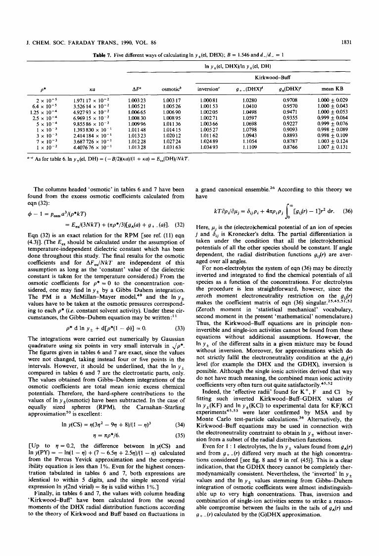
J. CHEM. SOC. FARADAY TRANS., 1990, VOL. 86 1831
Table 7. Five different ways of calculatingln y*(el, DHX); B = 1.546 and d + / d - = 1
~~
Kirkwood-Buff
P* KU AFa osmoticb inversion‘ g + -(DHX)d gA(DHX)e mean KB
2 x 10⁻⁵ 6.4 x 10⁻⁵
1.25 x 10⁻⁴ 2.5 x 10⁻⁴
5 x 10⁻⁴ 1 x 1 0 - 3 3 x 10⁻³ 7 x 10⁻³ 1 x
1.971 17 x lo-’ 3.52614 x lo-’ 4.92793 x lo-’ 6.96915 x lo-’ 9.85586 x lo-’ 1.393 830 x lo-’ 2.414184 x lo-’ 3.687726 x lo-’ 4.407676 x lo-’
~
1.003 23 1.005 21 1.006 65 1.008 30 1.009 96 1.01 148 1.013 23 1.012 28 1.013 28
1.003 17 1.005 26 1.006 90 1.008 95 1.01 1 36 1.014 15 1.020 12 1.027 24 1.03 1 63
1.OOO81 1.001 53 1.002 05 1.002 71 1.003 66 1.005 27 1.01 1 62 1.024 89 1.034 93
1.0280 1.0410 1 .M98 1.0597 1.0698 1.0798 1.0943 1.1054 1.1 109
0.9708 0.9570 0.9471 0.9355 0.9227 0.9093 0.8893 0.8787 0.8766
1.OOO f 0.029 1.OOO k 0.043 1.OOO f 0.053 0.999 f 0.064 0.999 f 0.076 0.998 f 0.089 0.998 f 0.109 1.003 f 0.124 1.007 _+ 0.131
a+ As for table 6. In y +(el, DH) = ( - B/~)(Ku)/( 1 + K U ) = E,,(DH)/NkT.
The columns headed ‘osmotic’ in tables 6 and 7 have been found from the excess osmotic coefficients calculated from eqn (32):
Eqn (32) is an exact relation for the RPM [see ref. (11) eqn (4.3)]. (The E,, should be calculated under the assumption of temperature-independent dielectric constant which has been done throughout this study. The final results for the osmotic coefficients and for A F J N k T are independent of this assumption as long as the ‘constant’ value of the dielectric constant is taken for the temperature considered.) From the osmotic coefficients for p* = 0 to the concentration con- sidered, one may find In y, by a Gibbs-Duhem integration. The PM is a McMillan-Mayer and the In y, values have to be taken at the osmotic pressures correspond- ing to each p* (i.e. constant solvent activity). Under these cir- cumstances, the Gibbs-Duhem equation may be written :11
(33) p* d In y , + d[p*(l - 4)] = 0.
The integrations were carried out numerically by Gaussian quadrature using six points in very small intervals in ,/p*. The figures given in tables 6 and 7 are exact, since the values were not changed, taking instead four or five points in the intervals. However, it should be underlined, that the In y , compared in tables 6 and 7 are the electrostatic parts, only. The values obtained from Gibbs-Duhem integrations of the osmotic coefficients are total mean ionic excess chemical potentials. Therefore, the hard-sphere contributions to the values of In y,(osmotic) have been subtracted. In the case of equally sized spheres (RPM), the Carnahan-Starling approximation5’ is excellent :
(34)
1 = np*/6. (35) [Up to q = 0.2, the difference between In y(CS) and In y(PY) = - ln(1 - 1) + (7 - 6.51 + 2.51)/(1 - 1) calculated from the Percus Yevick approximation and the compress- ibility equation is less than 1%. Even for the highest concen- tration tabulated in tables 6 and 7, both expressions are identical to within 5 digits, and the simple second virial expression In y(2nd virial) = 8q is valid within 1%.]
Finally, in tables 6 and 7, the values with column heading ‘Kirkwood-Buff have been calculated from the second moments of the DHX radial distribution functions according to the theory of Kirkwood and Buff based on fluctuations in
a grand canonical ensemble.26 According to this theory we have
k T d p , / a p j = 6 , p i + 4 n p i p j [gi,(r) - l]r2 dr. (36)
Here, pj is the (e1ectro)chemical potential of an ion of species j and d i j is Kronecker’s delta. The partial differentiation is taken under the condition that all the (e1ectro)chemical potentials of all the other species should be constant. If angle dependent, the radial distribution functions gi,.(r) are aver- aged over all angles.
For non-electrolytes the system of eqn (36) may be directly inverted and integrated to find the chemical potentials of all species as a function of the concentrations. For electrolytes the procedure is less straightforward, however, since the zeroth moment electroneutrality restriction on the g . {r) makes the coefficient matrix of eqn (36) s i n g ~ l a r . ~ ~ ~ ~ ~ . ~ ” , ~ ~ (Zeroth moment in ‘statistical mechanical’ vocabulary, second moment in the present ‘mathematical’ nomenclature.) Thus, the Kirkwood-Buff equations are in principle non- invertible and single-ion activities cannot be found from these equations without additional assumptions. However, the In y, of the different salts in a given mixture may be found without inversion. Moreover, for approximations which do not strictly fulfil the electroneutrality condition at the gi,(r) level (for example the DHX and the GDHX), inversion is possible. Although the single ionic activities derived that way do not have much meaning, the combined mean ionic activity coefficients very often turn out quite sa t i s fa~tor i ly .~~*’~
Indeed, the ‘effective radii’ found for K + , F- and C1- by fitting such inverted Kirkwood-Buff-GDHX values of In y*(KF) and In y*(KCl) to experimental data for KF/KCl experiment^^^,^^ were later confirmed by MSA and by Monte Carlo test-particle calculation^.^^ Alternatively, the Kirkwood-Buff equations may be used in connection with the electroneutrality constraint to obtain In y without inver- sion from a subset of the radial distribution functions.
Even for 1 : 1 electrolytes, the In y, values found from gA(r) and from g + - ( r ) differed very much at the high concentra- tions considered [see fig. 8 and 9 in ref. (45)]. This is a clear indication, that the GDHX theory cannot be completely ther- modynamically consistent. Nevertheless, the ‘inverted’ In y , values and the Iny, values stemming from Gibbs-Duhem integration of osmotic coefficients were almost indistinguish- able up to very high concentrations. Thus, inversion and combination of single-ion activities seems to strike a reason- able compromise between the faults in the tails of gA(r) and g + - ( r ) calculated by the (G)DHX approximation.
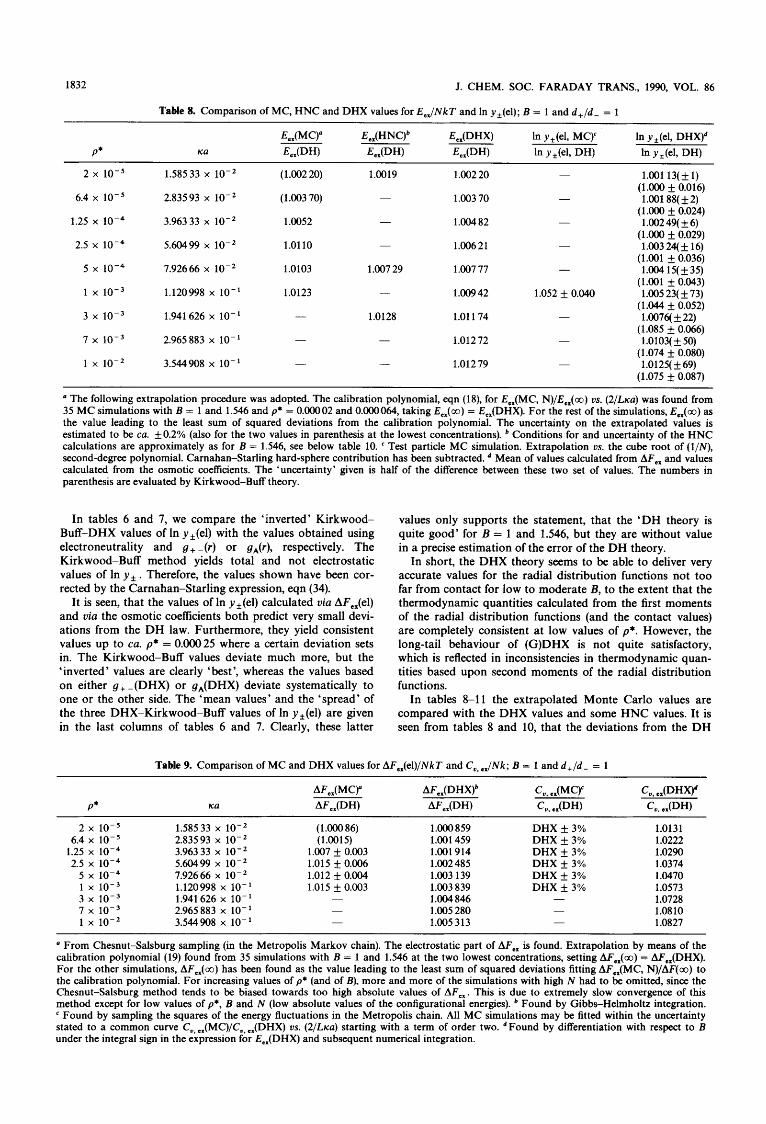
1832 J. CHEM. SOC. FARADAY TRANS., 1990, VOL. 86
Table 8. Comparison of MC, HNC and DHX values for E,,/NkT and In y+(el); B = 1 and d + / d - = 1
2 x 10⁻⁵
6.4 x 10⁻⁵
1.25 x 10⁻⁴
2.5 x 10⁻⁴
5 x 10⁻⁴
1 x 10⁻³
3 x 10⁻³
7 x 10⁻³
1 x lo-’
1.58533 x lo-’
2.83593 x lo-’
3.96333 x lo-’
5.60499 x lo-’
7.92666 x
1.120998 x lo-’
1.941626 x lo-’
2.965 883 x lo-’
3.544908 x lo-’
( 1.002 20) 1.0019
(1.003 70) -
1 .OO52 -
1.01 10
1.0103 1.007 29
1.0123 -
-
1.0128 -
1.002 20
1.003 70
1.004 82
1.006 21
1.007 77
1.009 42
1.01 174
1.01272
1.012 79
- 1.001 13( f 1) (1.OOO f 0.016) 1.001 88( f 2)
(1 .OOO f 0.024) 1.002 49( f 6)
(1.OOO f 0.029) 1.003 24(+ 16)
(1.001 f 0.036) 1.004 15( f35)
(1.001 f 0.043) 1.005 23( f 73)
(1.044 f 0.052) 1.0076( f 22)
(1.085 f 0.066) - 1.0103( & 50) - (1.074 f 0.080)
1.0123 f 69) (1.075 f 0.087)
-
-
-
-
1.052 0.040
-
The following extrapolation procedure was adopted. The calibration polynomial, eqn (18), for E,,(MC, N)/E,,(co) vs. (2/L~a) was found from 35 MC simulations with B = 1 and 1.546 and p* = 0.00002 and O.OOOO64, taking E,,(co) = E,,(DHX). For the rest of the simulations, E,,(co) as the value leading to the least sum of squared deviations from the calibration polynomial. The uncertainty on the extrapolated values is estimated to be ca. +0.2% (also for the two values in parenthesis at the lowest concentrations). Conditions for and uncertainty of the HNC calculations are approximately as for B = 1.546, see below table 10. Test particle MC simulation. Extrapolation vs. the cube root of (l/N), second-degree polynomial. Carnahan-Starling hard-sphere contribution has been subtracted. Mean of values calculated from AFex and values calculated from the osmotic coefficients. The ‘uncertainty’ given is half of the difference between these two set of values. The numbers in parenthesis are evaluated by Kirkwood-Buff theory.
In tables 6 and 7, we compare the ‘inverted’ Kirkwood- Buff-DHX values of In y*(el) with the values obtained using electroneutrality and g + -(r) or gA(r), respectively. The Kirkwood-Buff method yields total and not electrostatic values of In y , . Therefore, the values shown have been cor- rected by the Carnahan-Starling expression, eqn (34).
It is seen, that the values of In y*(el) calculated via AFex(el) and via the osmotic coefficients both predict very small devi- ations from the DH law. Furthermore, they yield consistent values up to ca. p* = O.OOO25 where a certain deviation sets in. The Kirkwood-Buff values deviate much more, but the ‘inverted’ values are clearly ‘best’, whereas the values based on either g+ -(DHX) or gA(DHX) deviate systematically to one or the other side. The ‘mean values’ and the ‘spread’ of the three DHX-Kirkwood-Buff values of In y*(el) are given in the last columns of tables 6 and 7. Clearly, these latter
values only supports the statement, that the ‘DH theory is quite good’ for B = 1 and 1.546, but they are without value in a precise estimation of the error of the DH theory.
In short, the DHX theory seems to be able to deliver very accurate values for the radial distribution functions not too far from contact for low to moderate B, to the extent that the thermodynamic quantities calculated from the first moments of the radial distribution functions (and the contact values) are completely consistent at low values of p*. However, the long-tail behaviour of (G)DHX is not quite satisfactory, which is reflected in inconsistencies in thermodynamic quan- tities based upon second moments of the radial distribution functions.
In tables 8-11 the extrapolated Monte Carlo values are compared with the DHX values and some HNC values. It is seen from tables 8 and 10, that the deviations from the DH
Table 9. Comparison of MC and DHX values for AF,,(el)/NkT and C , ,JNk; B = 1 and d + / d - = 1
P*
2 x 10-5 6.4 x 10⁻⁵
1.25 x 10⁻⁴ 2.5 x 10⁻⁴
5 x 10⁻⁴ 1 x 10⁻³ 3 x 10⁻³ 7 x 10⁻³ 1 x
1.58533 x 2.83593 x 3.96333 x 5.60499 x 7.92666 x lo-’ 1.120998 x lo-’ 1.941626 x lo-’ 2.965883 x lo-’ 3.544908 x lo-’
( 1 .OOO 86) 1.OOO 859
1.007 f 0.003 1.001 914 1.015 f 0.006 1.002 485 1.012 f 0.004 1.003 139 1.015 f 0.003 1.003 839
1.004 846 - 1.005 280 - 1.005 313
(1.0015) 1.001 459
-
DHX 3% 1.0131 DHX f 3% 1.0222 DHX f 3% 1.0290 DHX f 3% 1.0374 DHX f 3% 1.0470 DHX k 3% 1.0573 - 1.0728
1.0810 1.0827
- -
From Chesnut-Salsburg sampling (in the Metropolis Markov chain). The electrostatic part of AF,, is found. Extrapolation by means of the calibration polynomial (19) found from 35 simulations with B = 1 and 1.546 at the two lowest concentrations, setting AF,,(co) = AF,,(DHX). For the other simulations, AF,,(oo) has been found as the value leading to the least sum of squared deviations fitting AF,,(MC, N)/AF(oo) to the calibration polynomial. For increasing values of p* (and of B), more and more of the simulations with high N had to be omitted, since the Chesnut-Salsburg method tends to be biased towards too high absolute values of AF,,. This is due to extremely slow convergence of this method except for low values of p*, B and N (low absolute values of the configurational energies). Found by Gibbs-Helmholtz integration.
Found by sampling the squares of the energy fluctuations in the Metropolis chain. All MC simulations may be fitted within the uncertainty stated to a common curve Cu, ,,(MC)/Cu, ,,(DHX) 0s. ( 2 / L ~ a ) starting with a term of order two. Found by differentiation with respect to B under the integral sign in the expression for E,,(DHX) and subsequent numerical integration.

J. CHEM. SOC. FARADAY TRANS., 1990, VOL. 86 1833
Table 10. Comparison of MC, HNC and DHX values for E,,/NkT and In y,(el); B = 1.546 and d + / d - = 1 and 3
_ _ _ _ _ _ _ ~
2 x 10⁻⁵
6.4 x 10⁻⁵
1.25 x 10⁻⁴
2.5 x 10⁻⁴
5 x 10⁻⁴
1 x 10⁻³
3 x 10⁻³
7 x 10⁻³
1 x lo-’
1.971 17 x
3.52614 x lo-’
4.92793 x lo-’ 6.96915 x lo-’ 9.85586 x lo-* 1.393830 x lo-’ 2.414184 x lo-’ 3.687 726 x 10- ’ 4.407676 x lo-’
(1.006 58)
(1.010 80)
1.0134
1.0178
1.0209 [ 1.02351 1.023 5 [ 1.02691 -
1.0420
1.0048 f 0.0014
1.0096 f O.OOO6
1.0122 f o.oO04
1.0150 f 0.0003
1.0190 f 0.0002
1.0224 f 0.0001 C1.0253 f 0.0001) 1.0284 f 0.0002
c1.0212 f 0.00021
1.0362 rf: 0.0005
1.0403 f O.OOO6
1.006 58
1.01080
1.013 90
1.017 59
1.021 59
1.025 52
1.030 2 1
1.031 11
1.030 55
- 1.0020 f 0.0014
- 1.0046 f O.OOO6
- 1.0058 f O.oO04
- 1.0074 f 0.0002
- 1.0094 k 0.0002 Cl.0159 f 0.00021 1.01 19 f 0.0001 C1.0203 f 0.000ll
- 1.0170 f 0.0002
1.023 f 0.01 1 C1.024 f 0.0091
- 1.0255 f 0.0005
1.078 f 0.034 1.0306 f O.OOO6
1.003 2q f 3) (1.000 f 0.029) 1.005 24( f 3) (1 .OOO f 0.043) 1.006 78( f 13) (1.ooO k 0.053) 1.008 63( f 33) (0.999 f 0.064) 1.010 66( f 70) (0.999 f 0.076) 1.0128(+ 13) (0.998 f 0.089) 1.0167( f 35) (0.998 & 0.109) 1.0198( f 75) (1.003 f 0.124) 1.0225( f 92) (1.007 f 0.131)
a See below table 8 for the extrapolation procedure applied. Uncertainty estimated to ca. +0.2%. Values in square brackets correspond to d + / d - = 3. Filon integration using 8001 equidistant grid points in Fourier k-space. The maximum ka varied from 80 at the lowest concentra- tions to 1200 at the highest. Inside the hard-sphere ions, 10-20 equidistant grid points in t = r/a were used to represent the direct correlation function C..(r). The numbers of internal grid points necessary increase with concentration. A maximum of 3-4 iteration cycles in the HNC approximazon scheme were necessary for a precision corresponding to four significant digits. Often two iterations were sufficient. The indicated uncertainties are somewhat greater, since the values obtained varied slightly with the other parameters used in the HNC calculations. Values in square brackets correspond to d + / d - = 3. Test particle MC. Extrapolation us. the cube root of (l/N) (second-degree polynomial). Carnahan- Starling hard-sphere contribution has been subtracted. Values in square brackets correspond to d + / d - = 3. In y,(HNC) found directly by integration with respect to the Kirkwood coupling parameter using the special relations of the HNC theory, see ref. (37), (41) and (42). Camahan-Starling hard-sphere contribution subtracted. Values in square brackets correspond to d + / d - = 3. Mean between values calculated from AF,, and values calculated from osmotic coefficients. The ‘uncertainty’ indicated is half of the difference between these two sets of values. The numbers in parenthesis are evaluated by the Kirkwood-Buff theory.
law are almost identical for E,,(DHX) and E,,(HNC) up to ca. p* = 0.003. Also, for B = 1.546 the deviation from the DH law is almost identical for E,,(HNC) and for E,,(MC) even up to p* = 0.01. (The DHX model underestimates some- what the deviation at this ‘high’ concentration.)
It is also apparent from table 10, that lny,(HNC) and In y,(DHX) deviate almost identically from the DH law up to ca. p* = 0.005, whereas the test-particle values In y,(MC) in tables 8 and 10 support the direction in which the ‘true values’ deviate from the DH law, but is otherwise too uncer- tain to be of any help.
Tables 9 and 11 show that AF,,(DHX) deviate consider- ably less from the DH law than E,,(DHX). Table 11 demon- strates that DHX and HNC yield almost identical deviations at least up to p* = 0.001. The values of AF,,(HNC) have been found from In y,(HNC) = G,JNkT from which AF,,(HNC) may be found correcting for the osmotic coeffi- cient (the pV term). The Carnahan-Starling hard-sphere con- tribution has also been subtracted to obtain the electrostatic part of AF,JNkT, only. The MC values (Salsburg-Chesnut) should yield the electrostatic part directly for an ‘infinite number’ of steps.22 However, in practice, the uncertainty of
Table 11. Comparison of MC, HNC and DHX values for AF,,(el)/NkT and Cus ,JNk; B = 1.546 and d + / d - = 1 and 3
2 x 10⁻⁵ 6.4 x 10⁻⁵ 1.25 x 10⁻⁴ 2.5 x 10⁻⁴ 5 x 10⁻⁴
1 x 10⁻³
3 x 10⁻³ 7 x 10⁻³ 1 x
1.971 17 x lo-’ ( 1.002 47)
4.92793 x lo-’ 1.0118 f 0.0033 6.96915 x lop2 1.0165 f 0.0029 9.85586 x 1.0145 f 0.0032
C1.0230 f 0.00321 1.393830 x lo-’ 1.0181 f 0.0023
C1.0250 & 0.00311 2.414184 x lo-’ -
3.687726 x lo-’ - 4.407 676 x lo-’ -
3.52614 x (1.004 10) 1.001 66 1.003 56 1.004 69 1.006 15 1.00800 C1.012621 1.009 91 C1.016 161 1.013 60 1.019 21 1.022 58
1.002 47 1.004 10 1.005 30 1.006 76 1.008 38
1.010 01
1.012 09 1.01268 1.012 55
DHX f 3% DHX f 3% DHX f 3% DHX & 3% 1.12 f 0.03
[same for d + / d - = 31 1.15 rf: 0.03
[same for d + / d - = 31
- 1.25 f 0.06
1.0401 1.0664 1.0850 1.1081 1.1334
1.1589
1.1926 1.2047 1.2049
See below table 9 for the extrapolation procedure applied. Values in square brackets correspond to d + / d - = 3. In y,(HNC) found directly by integration with respect to the Kirkwood coupling parameter using the special relations of the HNC theory, see ref. (37), (41) and (42). From this is calculated the excess Gibbs’ free energy G,,/NkT. This quantity combined with the osmotic coefficient in the HNC approximation leads to F,,(HNC)/NkT. Subtracting the Carnahan-Starling hard-sphere contribution to F,JNkT, the electrostatic Helmholtz free energy AF,,(HNC)/NkT is found. The values in square brackets correspond to d + / d - = 3. Found by Gibbs-Helmholtz integration. See below table 9. The values of C,,,,(N = oo)/Nk for B = 1.546 and p* = 0.0005 and 0.001 seem to be ca. 2% lower than the DHX values, however. The same is true for d + / d - = 3. See fig. 17. Found by differentiation under the integral sign in the expression for E,,(DHX) and subsequent numerical integration.
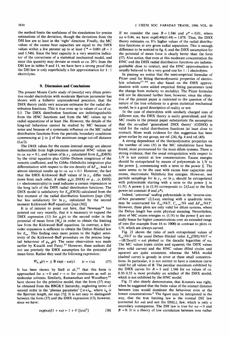
1834 J. CHEM. SOC. FARADAY TRANS., 1990, VOL. 86
the method limits the usefulness of the simulations for precise estimations of the deviation, though the deviations from the DH law are at least in the ‘right’ direction. Finally, the MC values of the excess heat capacities are equal to the DHX values within a few percent up to at least C* = 0.001 ( B = 1 and 1.546). Since the heat capacity is a very sensitive indica- tor of the correctness of a statistical mechanical model, and since this quantity may deviate as much as ca. 20% from the DH law in tables 9 and 11, we have here a strong proof that the DH law is only superficially a fair approximation for 1 : 1 electrolytes.
9. Discussion and Conclusions The present Monte Carlo study of (mostly) very dilute primi- tive model electrolytes with moderate Bjerrum parameter has shown with a hitherto unprecedented precision, that the DHX theory yields very accurate estimates for the radial dis- tribution functions. This is true even up to values of k-a of ca. 0.5. The DHX distribution functions are indistinguishable from the HNC functions and from the MC values up to radial separations of at least 10a. However, the details of the long-tail behaviour cannot be studied by MC because of noise and because of a systematic influence on the MC radial distribution functions from the periodic boundary conditions commencing at 3 to 4 of the minimum image cut-off distance (Ld2).
The DHX values for the excess internal energy are almost indiscernible from high-precision numerical HNC values up to ca. k-a = 0.1, and values of In y , calculated from E,,(DHX) by the virial equation plus Gibbs-Duhem integration of the osmotic coefficient, and by Gibbs-Helmholtz integration plus differentiation with respect to the ion density of AF,,, lead to almost identical results up to ca. k-a = 0.1. However, the fact that the DHX-Kirkwood-Buff values of In y , differ much more from each other, if either gA(t-9 DHX) or g+ -(r, DHX) (+ electroneutrality) is used indicates a certain imprecision in the long tails of the DHX radial distribution functions. The DHX model is satisfactory for E,,(DHX) calculated from the first moment of the radial distribution functions [eqn (20)] but less satisfactory for In y, calculated by the second moment Kirkwood-Buff equations [eqn (36)].
It is of interest to point out here, that NewmanS4 has pointed out very recently, that it is necessary to expand the DHX expression (11) for g&) to the second order in the potential of mean force (Ki> in order to obtain the limiting law from the Kirkwood-Buff equations. In contrast, a first- order expansion is sufficient to obtain the Debye-Huckel law for Eex. This finding once more points to the higher sensi- tivity of the Kirkwood-Buff procedure on the precise long- tail behaviour of gA, B ( ~ ) . The same observation was made earlier by Kusalik and Patey.” However, these authors did not use precisely the DHX assumption for the potential of mean force. Rather they used the following expression :
It has been shown by Stell et al.,’’ that this form is approached for K -+ 0 and r + m for continuum as well as molecular solvents. Similarly, Ramanathan and W ~ o d b u r y ~ ~ have shown for the primitive model, that the form (37) may be obtained from the BBGKY hierarchy, neglecting terms of second order in the ‘plasma parameter’ [ 3 K& , where ,IB is the Bjerrum length, see eqn (7)]. It is not easy to distinguish between the form (37) and the DHX expression (12), however, since we have :
If we consider the case B = 1.546 and p* = 0.01, where KU M 0.44, we have exp(0.44)/(1.44) = 1.078. Thus, the DHX theory estimates ca. 8% higher values of the radial distribu- tion functions at any given radial separation. This is enough difference to be noticed in fig. 6, and the DHX assumption for the potential of mean force is clearly better than the form (37). Also notice, that even at this moderate concentration the HNC and the DHX radial distribution functions are indistin- guishable close to contact, and the HNC approximation is usually believed to be a very good one for 1 : 1 electrolytes.
In passing we notice that the semi-empirical formulae of Pitzer used for fitting thermodynamic properties of electro- lyte s o l u t i ~ n s ~ ~ - ~ ~ are also based on the DHX approx- imation with some added empirical fitting parameters (and the change from molarity to molality). The Pitzer formulae will not be discussed further here, however, since the objec- tive of the present paper is restricted to the question of the nature of the true solutions to a given statistical mechanical model, be it a good description of reality or not.
In the case of electrolytes with similarly charged ions of different size, the DHX theory is easily generalized, and the MC results in the present paper substantiate the assumption that the so-called ‘generalized DHX theory’ (GDHX) is valid for the radial distribution functions (at least close to contact). More weak evidence for this suggestion has been given earlier by our group, see ref. (24), fig. 4 and ref. (45).
A strong dependence of the thermodynamic properties on the number of ions ( N ) in the MC simulations have been found, most pronounced for the most dilute systems. There is strong evidence, that the usual extrapolation with respect to 1/N is not correct at low concentrations. Excess energies should be extrapolated by means of polynomials in 1/N to the power 3, commencing with a term to the power 3. The same seems to be the case with excess heat capacities and excess, electrostatic Helmholz free energies. However, test particle samplings for In y, or In yi should be extrapolated with polynomials starting with a term to the power 5 in (l/N). A power 4 in (l/N) corresponds to 2/(Lk-a) to the first power (at constant B and p*).
Indeed, ‘universal ’ scaling polynomials in the ‘ inverse-size- of-box parameter’ (2/Lk-a), starting with a quadratic term, may be constructed for E,JNkT, C, , ,JNk and AF,JNkT. However, these plots are only valid for dilute systems, where the Debye length has some physical meaning. Nevertheless, plots of MC excess energies us. (l/N) to the power 4 are nor- mally linear for higher concentrations over an extended range of ions (for example from 16 to 1OOO) in contrast to plots us. 1/N, which are always curved.
Fig. 21 shows the ratio of such extrapolated values of E,,/NkT to the usual Debye-Huckel value E,,(DH)/NkT = -(B/2)~a/(l + K U ) plotted us. the decadic logarithm of k-a. The MC values (open circles and squares), the DHX values (two solid curves) and the HNC values (filled circles and squares) are quite consistent, whereas the MSA model (dashed curve) is grossly in error at these small concentra- tions. In particular, it is not correct to have a common curve valid for all values of B. The peculiar maximum exhibited by the DHX curves for B = 1 and 1.546 for KU values of ca. 0.304.35 is most probably an artefact of the DHX model, which is not exhibited by the HNC model.
Fig. 21 also clearly demonstrates, that Kramers was right, when he suggested that the finite value of the contact distance between ions would dominate the behaviour even at the lowest concentration^.^ The figure may be interpreted in the way, that the true limiting law is the normal DH law (corrected for k-a) and not the DHLL law, which is only a secondary consequence. The DH law is true for k-a-+O and B + 0 . It is a theory of low correlation between ions rather

J. CHEM. SOC. FARADAY TRANS., 1990, VOL. 86
1.05
1.01
1835
I - I
I HNC I I O:
- I ?I'
than a theory of low concentrations. More precisely expressed, the plasma parameter BKU has to be low as stressed also by Ramanathan and W o o d b ~ r y . ~ ~ The status of the DH law as such a limiting law of low correlation is evident, if the DHX model is assumed correct, since the DH law for E,, (and not the DHLL law) follows by expanding the radial distribution functions to the first term in the DHX potential of mean force.
Fig. 22 shows similar relative plots for the excess heat capacity. The deviations from the DH expression (B/~)Ku/ [l + are much more pronounced for this quantity, but still the suggestion is supported that the DH law is the true limiting law of low correlation (low BKU). However, because of the large deviations from the DH law, it may happen (as for B = 1.546) that the DHLL law is followed quite closely at low concentrations.
Fig. 23 exhibits relative plots for the excess, electrostatic Helmholtz free energy. The DHX curves [calculated from E,,(DHX) by Gibbs-Helmholtz integration] show the same split-up for different values of B as shown by the other ther- modynamic quantities. This is not the case for the MC values. Probably, this is due to the deficiencies of the Salsburg-Chesnut method, which requires longer runs, espe- cially for B = 1 where most of the simulations were sampled
1.301
0.01 0.0210.03-0.05 0.10 0.200.30 0.50 Ka
1 Fig. 22. Plot of C", ,,/CU, ,,(DH) us. KQ. [C,, ,,(DH)/Nk = (B/~)(KQ)/ (1 + KU)']. The solid curves calculated by the DHX theory corre- spond to the two Bjerrum parameters [(a) 1.546; (0) 1). The Monte Carlo values are statistically indistinguishable from the DHX values, except perhaps the three highest concentrations for B = 1.546 @* = 0.0005, 0.001 and 0.01). Triangles (A) correspond to B = 1.546, d+/d- = 3. Statistically, there is no difference between d+/d- = 3 and d + / d - = 1, see fig. 17. The deviation from the DH law is much larger for C , , , than for E,,. Indeed, the deviation is so large for B = 1.546 that the values fortuitously come close to DHLL, when KQ -+ 0. Still, however, the DH law is the true limiting law for KQ -+ 0 and B -+ 0. The strong deviation of C,, ex from the DH value is a strong indication that the DH law is only superficially a working theory for large 1 : 1 electrolytes in solution at room temperature. Severe problems will arise for higher values of B (2 : 1 and 2 : 2 electrolytes) also for the other thermodynamic properties. Notice once more the peculiar maxima of the DHX curves around KQ = 0.35.
over 'only' 2 million configurations. Nevertheless, when the MC values are correctly extrapolated, they are at least situ- ated between the DH values and the DHLL values. Thus, the 'overshoot' to the 'wrong' side of DHLL reported earlier [ref. (22), fig. 6; ref. (23), fig. 5(b)] seems to be a consequence of wrong extrapolation and an insuficient number of con- figurations for the simulations with many ions.
Fig. 24 shows relative plots for the electrostatic contribu- tion to In y, . For the DH theory, we have In y,(el, DH) = E,,(DH)/NkT. We observe once more the split-up into curves for each value of B. The HNC values for B = 1.546 (dotted curve and filled squares) are probably close to the truth. These values correspond well with the DHX values calcu- lated by the virial theorem, Gibbs-Duhem integration of the osmotic coefficient and correction for the hard-sphere contri- bution. Up to ca. Ica = 0.10 there is also reasonable agree- ment with the values calculated by the Gibbs-Helmholtz route. The two extrapolated MC values calculated by the test particle method for B = 1.546, p* = 0.001 and d + / d - = 1 and 3 have not been plotted here, since the uncertainty is too great to be of much help in the present, very sensitive, plot.
It should be noticed, that if one thinks that the primitive model is describing the first deviation from the limiting laws in real electrolyte solutions, and if one simply fits the DH equation for In y , with the hard-sphere terms added, as we did,61 then we obtain values of the effective ionic radii that

1836
T
n I
4
1.020
1.015
1.010
1.005
1.000 0.01 0.02 0.05 0.10 0.20 0.50 1.0
hz
Fig. 23. Plot of AF,JAF,,(DH) us. KU. AF,,(DH)/NkT = [ -B/(~a)’]fln(l + K U ) - KU + (~a )~ /2 ] . The DHX values [calculated from E,,(DHX) by Gibbs-Helmholtz integration with respect to B ] follows for B = 1.546 (upper solid curve) the HNC values (m) closely (except for the peculiar maximum in the DHX curve around KU = 0.35). The Monte Carlo data are somewhat unclear, but this may easily be due to the lack of precision of the Salsburg-Chesnut method. In particular, the absolute values of AF,,(MC) for B = 1 might be somewhat too high [compare the MC values (0) to the lower DHX curve], since these runs were ‘only’ extended to 2 million configurations, whereas most of the B = 1.546 runs were longer. Probably, the HNC values (or the DHX values up to KU = 0.2) are near to the truth. In general, the deviation of the electrostatic part of the excess Helmholtz free energy from the DH law seems to be only ca. one-half of the deviation of the excess energy. As deemed from HNC, the value for AF,, is increased relatively more than E,, for unequal ionic diameters. MC symbols: B = 1 (0); B = 1.546, d + / d - = 1 (n), d + / d - = 3 (A). HNC symbols: B = 1.546, (m) d + / d - = 1, (A) d + / d - = 3.
are too small. This is so, since fig. 24 shows that the DH equation for In y * overestimates the electrostatic contribu- tion to the deviation from the limiting law, and since the elec- trostatic DH deviation and the hard-sphere deviation are in the same direction.
The influence of unequal ionic radii has been studied for B = 1.546 and two different concentrations (p* = 0.0005 and 0.001). A summary is given in table 12. It is seen, that the excess energy and the electrostatic, excess Helmholtz free energy are increased a little in absolute value when the cation (anion) is made three times greater than the anion (cation), keeping the contact distance between the cation and the anion constant. This feature is evident in the MC data as well as in the HNC and MSA calculations. The absolute values of In yi seem to decrease for the ion made greater and to increase for the ion made smaller. However, all thermodyna- mic properties change very little indeed, when one considers
J. CHEM. SOC. FARADAY TRANS., 1990, VOL
i 1.030
1.025
I I I I I
t I 1 . o x
-7
1.010 t -
L
86
0.01 0.02 0.03 0.05 0.10 0.20 0.30 0.50 1.0
lca
Fig. 24. Plot of In y,(el)/ln y,(el, DH) vs. KU. In y,(el, DH) = ( - B/2x~a)/( 1 + KU). Solid curves : DHX theory by differentiation of AF,, (Gibbs-Helmholtz integration) with respect to concentration (upper, B = 1.546; lower, B = 1). Dashed curves: DHX through osmotic coefficients and Gibbs-Duhem integration (upper, B = 1.546; lower, B = 1). Subtraction of Camahan-Starling hard- sphere contribution. Dotted curve and .: HNC, B = 1.546. A: HNC, B = 1.546 and d + / d - = 3. The Gibbs-Helmholtz and the Gibbs-Duhem values agree reasonably up to KU = 0.07. As deemed from the HNC values, the DHX-Gibbs-Duhem values are very near the truth. They do not exhibit the peculiar maximum of the DHX- Gibbs-Helmholtz values. The general picture is similar to that for E,, , Cv, and AF,, with the DH law as the true limit for B -+ 0 and KU -+ 0. As for AF,,, the deviation from the DH law is only around one-half of the deviation of E,, . The DHLL is practically inaccessible at the present moderate B values. There is a great increase at B = 1.546 in the values of In y,(el)/ln y,@H) for unequal radii as judged from the HNC values. However, the total values of In y, are almost not changing because of counterbalancing hard-sphere effects, see also fig. 20.
the drastic alteration. In a recent HNC study of single-ion activity coefficients of PM 1 : 1 and 2 : 1 electrolyte^,^^ we have also found that the single-ion activity coefficients were largely unaffected by the relative sizes of the ions in the low concentration limit. Thus, whereas the ionic charges were very important in the discrimination of the two single-ion activities, only the contact distance between the positive and the negative ions matters in dilute solutions. Put another way, in dilute solutions of single electrolytes it is sufficient to solve the restricted primitive model with all ionic radii equal.
It is probably a very good assumption for dilute 1 : 1 elec- trolyte solutions to put In y , = In y - = In y , . This is impor- tant to know, when using and calibrating ion-selective
Table 12. The effect of different ionic sizes at B = 1.546 and two different concentrations
100 (-E,JNkT) 100 ( - AK,, ,,/NkT) 100 (-In Y**tOmJ 100 (-In Y-.*,ui)
P* d + / d - MC HNC MSA MC HNC MSA MC HNC MSA MC HNC MSA
6.793 6.740 0.0005 1 7.080 f 0.005 7.067 6.949 4.800 f 0.015 4.769 4.737 - 0.0005 3 7.098 f 0.005 7.082 6.981 4.840 f 0.015 4.791 4.765 - 6.706 6.611 - 6.808 6.824
0.001 1 9.678 f 0.005 9.668 9.492 6.625 k 0.015 6.572 6.522 9.26 f 0.11 9.150 9.073 9.26 f 0.11 9.150 9.073 0.001 3 9.711 f0.005 9.695 9.555 6.670 f 0.020 6.612 6.578 9.07 f 0.14 8.967 8.816 9.14 f 0.17 9.176 9.233
- 6.793 6.740

J. CHEM. SOC. FARADAY TRANS., 1990, VOL. 86 1837
electrodes. In the case of higher concentrations, Sloth and Snrrensen3 found significant differences between the single- ion activities of the two ions, when one ion was made three times greater than the other at a fixed Bjerrum parameter (B = 1.681).
In summary, except for C,,,,, very small, though signifi- cant deviations from the DH theory are found for dilute systems at moderate Bjerrum parameters. The deviations are well described by the DHX and the HNC theories. For higher values of B (2 : 2 electrolytes for example), we would expect much more pronounced deviations from the DH theory, and the DHX and HNC will most probably fail to estimate these deviations correctly. However, a method has now been established for extrapolating MC data, which might also be used for dilute systems for higher values of B. Presently, a very dilute system with B = ca. 6.8 are simulated together with some systems with B = 2 and also a very dilute
system of 2 : 1 electrolytes with B = 2 x 1.546. In a later paper, the final results of these simulations will be presented.
The author is indebted to the following persons with whom he has had productive discussions. Professor L. Blum (University of San Juan, Puerto Rico), Professor G. V. Rama- nathan (University of Illinois at Chicago) and Dr P. Sloth, Dr J. B. Jensen and Dr B. Malmgren-Hansen (Technical Uni- versity of Denmark). Dr H. B. Nielsen (previously Radi- ometer A/S) and Dr H. B. Kristensen (Radiometer A/S) are gratefully acknowledged for running some of the Monte Carlo simulations on the VAX 11/750 of Radiometer A/S. Last, but not least, the author is indebted to economic support during the years from Teknologistyrelsen (The Danish National Agency of Technology) and from Statens Naturvidenskabelige Forskningsrid, Otto Msnsteds Fond and Thomas B. Thriges Fond.
Appendix: Monte Carlo Data
Table Al. Bjerrum parameter B = 1 ; equal ionic diameters ~~~ ~ ~
millions - 100 In y + - 100 In y - g+ -(r), g,,(r) N of configs. - 100E(ex)/NkT" - 100AF(ex)/NkTb + 100C,(ex)/NkTc (test) (test) in range" computere
64
100
150
216
3 50
512
700
loo0
64
100
150
216
350
512
700
loo0
64
100
150
216
5.00
2.00
2.00
2.00
2.00
2.00
2.00
1 .00
3.00
2.00
2.00
2.00
2.00
2.00
2.00
1 .00
2.00
2.00
2.00
2.00
1.064
0.9899
0.9417
0.8994
0.8610
0.8447
0.8272
0.8144
1.719
1.623
1.558
1.505
1.483
1.458
1.441
1.422
2.284
2.168
2.099
2.039
p* = 0.00002 0.9367
0.8478
0.7859
0.7310
0.6834
0.6469
0.5943
0.5981
p* = o.oo0064 1.466
1.340
1.247
1.181
1.121
1.072
1.063
0.9555
p* = O.oo0 125 1.904
1.752
1.654
1.570
K a = 1.58533 x lop2 0.2418
0.2667
0.2912
0.3067
0.3210
0.3525
0.3716
0.3661
K a = 2.83593 x lo-* 0.4740
0.5197
0.5597
0.5804
0.6209
0.6609
0.6457
0.6976
Ka = 3.96333 x 0.7027
0.7618
0.79 18
0.8324
a 4 a (2.55, 0.47)
a 4 a (2.24, 0.31)
a 4 a (2.93, 0.36)
a 4 a (2.51, 0.32)
a 4 a (2.55, 0.42)
a 4 a (2.56, 0.27)
a 4 a (2.58, 0.48)
a 4 a (2.53, 0.18)
a 4 a (2.15, 0.46)
a 4 a (2.79, 0.39)
a 4 a (2.56, 0.48)
a-4a (2.34, 0.28)
a-4a (2.34, 0.39)
a 4 a (3.13, 0.44)
a 4 a (2.25, 0.47)
a 4 a (2.32, 0.52)
a+ (2.34, 0.47)
a 4 a (2.57, 0.48)
a 4 a (2.14, 0.36)
a 4 a (2.59, 0.45)
AT
VAX
VAX
VAX
VAX
VAX
VAX
VAX
AT
VAX
VAX
VAX
VAX
VAX
VAX
VAX
AT
VAX
VAX
VAX
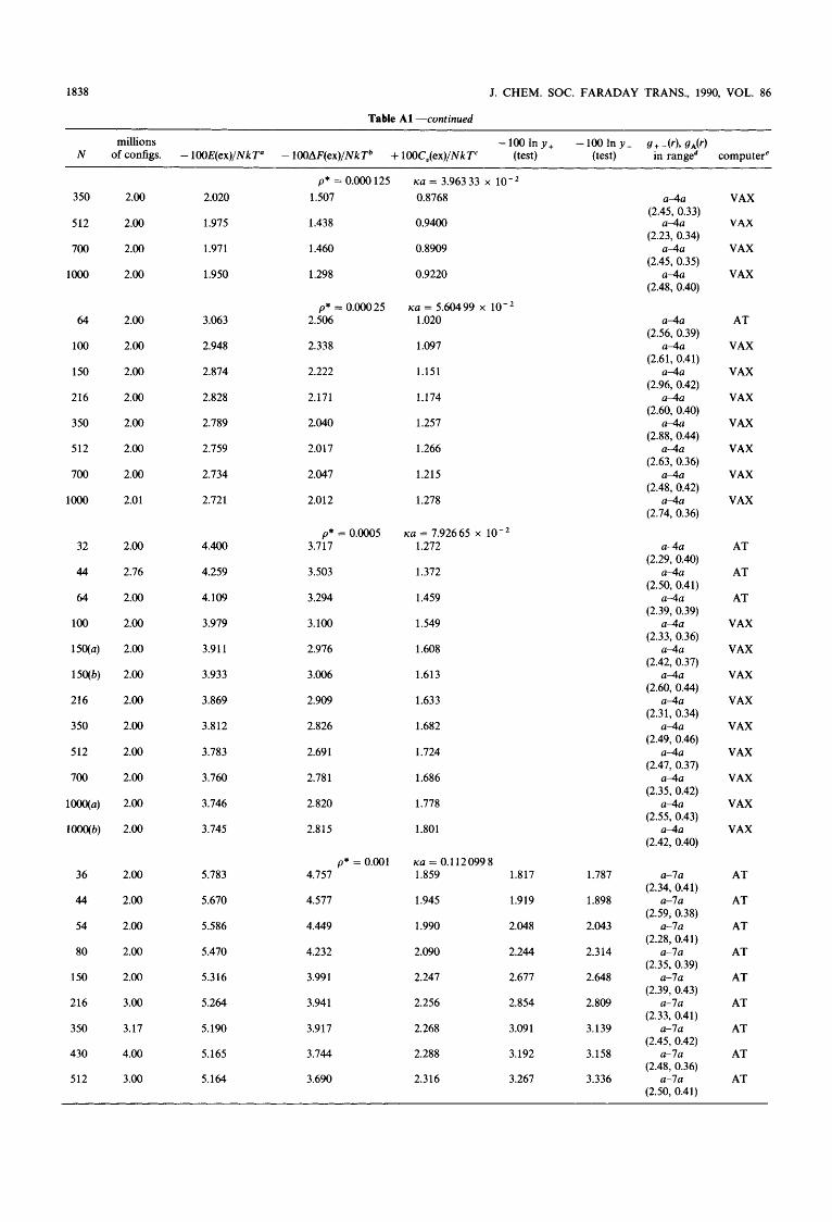
1838 J. CHEM. SOC. FARADAY TRANS., 1990, VOL. 86
Table A l -continued
millions - 100 In y , - 100 In y - g + 49, gA(r) N of configs. - 100E(ex)/NkT" - 100AF(ex)/NkTb + 100C,(ex)/NkT' (test) (test) in ranged computere
p* = 0.000 125 1.507
ua = 3.96333 x
0.8768 3 50
512
700
1000
64
100
150
216
3 50
512
700
1000
32
44
64
100
150(a)
15W)
216
3 50
512
700
1 W a )
1 ooo(b)
36
44
54
80
150
216
3 50
430
512
2.00
2.00
2.00
2.00
2.00
2.00
2.00
2.00
2.00
2.00
2.00
2.01
2.00
2.76
2.00
2.00
2.00
2.00
2.00
2.00
2.00
2.00
2.00
2.00
2.00
2.00
2.00
2.00
2.00
3.00
3.17
4.00
3 .OO
2.020
1.975
1.971
1.950
3.063
2.948
2.874
2.828
2.789
2.759
2.734
2.721
4.400
4.259
4.109
3.979
3.91 1
3.933
3.869
3.812
3.783
3.760
3.746
3.745
5.783
5.670
5.586
5.470
5.316
5.264
5.190
5.165
5.164
a 4 a (2.45, 0.33)
a 4 a (2.23, 0.34)
a 4 a (2.45, 0.35)
a 4 a (2.48, 0.40)
a 4 a (2.56, 0.39)
a 4 a (2.61, 0.41)
a-4a (2.96, 0.42)
a 4 a (2.60, 0.40)
a 4 a (2.88, 0.44)
a 4 a (2.63, 0.36)
a-4a (2.48, 0.42)
a 4 a (2.74, 0.36)
a 4 a (2.29, 0.40)
a 4 a (2.50, 0.41)
a 4 a (2.39, 0.39)
a 4 a (2.33, 0.36)
a-4a (2.42, 0.37)
a 4 a
a 4 a (2.31, 0.34)
a-4a (2.49, 0.46)
a-4a (2.47, 0.37)
a 4 a (2.35, 0.42)
a 4 a (2.55, 0.43)
a 4 a (2.42, 0.40)
a-7a (2.34, 0.41)
a-7a (2.59, 0.38)
a-7a (2.28, 0.41)
a-7a (2.35, 0.39)
a-7a (2.39, 0.43)
a-7a (2.33, 0.41)
a-7a (2.45, 0.42)
a-7a (2.48, 0.36)
a-7a (2.50, 0.41)
(2.60, 0.44)
VAX
VAX
VAX
VAX
AT
VAX
VAX
VAX
VAX
VAX
VAX
VAX
AT
AT
AT
VAX
VAX
VAX
VAX
VAX
VAX
VAX
VAX
VAX
AT
AT
AT
AT
AT
AT
AT
AT
AT
0.9400 1.438
1.460
1.298
0.8909
0.9220
ua = 5.60499 x lo-' 1.020
p* = 0.00025 2.506
1.097 2.338
2.222
2.171
1.151
1.174
2.040 1.257
2.017
2.047
1.266
1.215
2.0 12 1.278
p* = 0.0005 3.717
K a = 7.92665 x 1.272
3.503 1.372
3.294 1.459
3.100
2.976
1.549
1.608
1.613 3.006
2.909 1.633
1.682 2.826
2.69 1 1.724
2.781
2.820
1.686
1.778
2.815 1.801
p* = 0.001 4.757
K a = 0.1120998 1.859 1.817 1.787
1.898
2.043
2.314
2.648
2.809
3.139
3.158
3.336
4.577 1.945 1.919
1.990 2.048 4.449
4.232 2.090 2.244
3.99 1 2.247 2.677
3.941
3.917
2.256 2.854
2.268 3.09 1
3.744 2.288 3.192
3.690 2.316 3.267
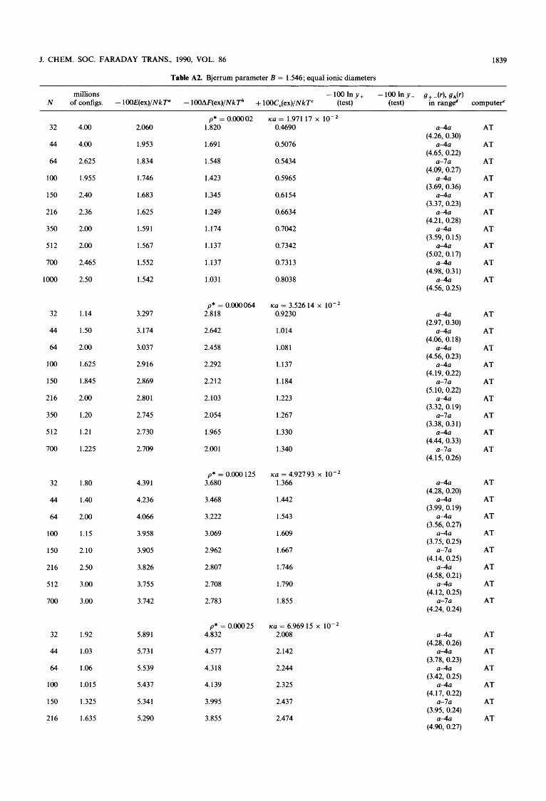
J. CHEM. SOC. FARADAY TRANS., 1990, VOL. 86 1839
Table A2. Bjerrum parameter B = 1.546; equal ionic diameters
millions - 100 In y , - 100 In y - g+ -(r) , g,(r) N of configs. - lOOE(ex)/NkT" - 100AF(ex)/NkTb + 100C,(ex)/NkTc (test) (test) in range" computere
32
44
64
100
150
216
3 50
512
700
1000
32
44
64
100
150
216
3 50
512
700
32
44
64
100
150
216
512
700
32
44
64
100
150
216
4.00
4.00
2.625
1.955
2.40
2.36
2.00
2.00
2.465
2.50
1.14
1.50
2.00
1.625
1.845
2.00
1.20
1.21
1.225
1.80
1.40
2.00
1.15
2.10
2.50
3 .00
3.00
1.92
1.03
1.06
1.015
1.325
1.635
2.060
1.953
1.834
1.746
1.683
1.625
1.591
1.567
1.552
1.542
3.297
3.174
3.037
2.916
2.869
2.801
2.745
2.730
2.709
4.39 1
4.236
4.066
3.958
3.905
3.826
3.755
3.742
5.89 1
5.731
5.539
5.437
5.341
5.290
p* = 0.00002 1.820
1.691
1.548
1.423
1.345
1.249
1.174
1.137
1.137
1.03 1
p* = 0.000064 2.818
2.642
2.458
2.292
2.212
2.103
2.054
1.965
2.001
p* = 0.000 125 3.680
3.468
3.222
3.069
2.962
2.807
2.708
2.783
p* = 0.00025 4.832
4.577
4.3 18
4.139
3.995
3.855
Ka = 1.971 17 x 0.4690
0.5076
0.5434
0.5965
0.6154
0.6634
0.7042
0.7342
0.7313
0.8038
K a = 3.526 14 x 0.9230
1.014
1.08 1
1.137
1.184
1.223
1.267
1.330
1.340
K a = 4.92793 x 1.366
1.442
1.543
1.609
1.667
1.746
1.790
1.855
K a = 6.969 15 x l op2 2.008
2.142
2.244
2.325
2.437
2.474
a 4 a (4.26, 0.30)
a 4 a (4.65, 0.22)
a-7a (4.09, 0.27)
a-4a (3.69, 0.36)
a-4a (3.37, 0.23)
a 4 a (4.21, 0.28)
a 4 a (3.59, 0.15)
a-4a (5.02, 0.17)
a 4 a (4.98, 0.31)
a 4 a (4.56, 0.25)
a 4 a (2.97, 0.30)
a-4a (4.06, 0.18)
a 4 a (4.56, 0.23)
a 4 a (4.19, 0.22)
a-7a (5.10, 0.22)
a 4 a (3.32, 0.19)
a-7a (3.38, 0.31)
a-4a (4.44, 0.33)
a-7a (4.15, 0.26)
a 4 a (4.28, 0.20)
a 4 a (3.99, 0.19)
a 4 a (3.56, 0.27)
a 4 a (3.75, 0.25)
a-7a (4.14, 0.25)
a 4 a (4.58, 0.21)
a 4 a (4.12, 0.25)
a-7a (4.24, 0.24)
a 4 a (4.28, 0.26)
a-4a (3.78, 0.23)
a 4 a (3.42, 0.25)
a 4 a (4.17, 0.22)
a-7a (3.95, 0.24)
a-4a (4.90, 0.27)
AT
AT
AT
AT
AT
AT
AT
AT
AT
AT
AT
AT
AT
AT
AT
AT
AT
AT
AT
AT
AT
AT
AT
AT
AT
AT
AT
AT
AT
AT
AT
AT
AT
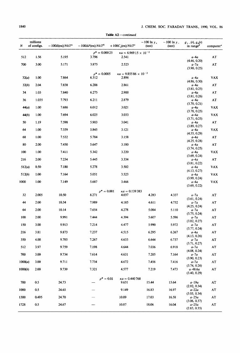
1840 J. CHEM. SOC. FARADAY TRANS., 1990, VOL. 86
Table A2 -continued
millions - 100 In y, - 100 In y- g+ -(r), gA(r) N of configs. - 100E(ex)/NkTa - 100AF(ex)/NkTb + 100C,(ex)/NkT' (test) (test) in ranged computere
512
700
3W)
3W)
34
36
44(4
Wb)
50
64
68
80
100
216
512(a)
5 lab)
1000
32
44
64
100
150
216
350
512
700
1 W4
1 W b )
700
lo00
1300
1728
1.56
3.00
1 .00
2.04
1.03
1.035
1 .00
1 .00
1.19
1 .00
1 .00
2.00
1 .OO
2.00
0.50
1 .OO
1 .00
2.005
2.00
2.00
2.00
3.00
3.8 1
4.00
3.97
3.00
3.00
2.00
0.5
0.5
0.495
0.5
5.195
5.171
7.864
7.838
7.840
7.793
7.686
7.694
7.598
7.559
7.532
7.450
7.41 1
7.234
7.180
7.164
7.149
10.50
10.34
10.14
9.99 1
9.9 13
9.873
9.785
9.759
9.734
9.71 1
9.739
24.73
24.65
24.70
24.67
p* = 0.00025 3.796
3.875
p* = 0.0005 6.312
6.288
6.275
6.21 1
6.012
6.025
5.903
5.845
5.784
5.647
5.342
5.445
5.278
5.05 1
5.687
p* = 0.001 8.271
7.989
7.654
7.444
7.214
7.237
7.267
7.198
7.614
7.734
7.321
p* = 0.01 -
Ka = 6.969 15 x lo-' 2.541
2.523
Ka = 9.85586 x lop2 2.896
2.861
2.900
2.879
3.021
3.033
3.041
3.121
3.158
3.180
3.220
3.334
3.502
3.523
3.466
Ka = 0.139 383 4.037
4.185
4.278
4.394
4.477
4.5 15
4.633
4.644
4.63 1
4.672
4.577
Ka = 0.440768 9.63 1
9.149
10.89
10.87
4.283
4.61 1
5.084
5.607
5.990
6.295
6.644
7.036
7.205
7.456
7.2 19
15.44
16.83
17.03
18.06
4.337
4.732
5.110
5.596
5.972
6.267
6.737
6.918
7.164
7.4 16
7.473
15.64
16.97
16.58
16.04
a 4 a (4.46, 0.20)
a-7a (3.90, 0.25)
a 4 a (4.86, 0.30)
a 4 a (3.81, 0.25)
a 4 a (3.81, 0.26)
a 4 a (3.70, 0.21)
a 4 a (3.78, 0.25)
a 4 a (3.71, 0.25)
a 4 a (3.89, 0.27)
a 4 a (4.55, 0.29)
a 4 a (4.25, 0.28)
a 4 a (3.74, 0.25)
a 4 a (3.69, 0.24)
a 4 a (3.81, 0.22)
a 4 a (4.13, 0.27)
a 4 a (3.99, 0.24)
a 4 a (3.69, 0.22)
a-7a (3.61, 0.24)
a-7a (4.25, 0.24)
a-7a (3.75, 0.24)
a-7a (3.82, 0.27)
a-7a (3.77, 0.24)
a 4 a (4.13, 0.26)
a-7a (3.71, 0.27)
a-7a (4.08, 0.24)
a-7a (3.90, 0.23)
a-7a (3.74, 0.26)
a48.6a (3.40, 0.29)
a-1 9a (2.92, 0.34)
a-22a (3.03, 0.34)
a-25a (3.06, 0.37)
a-25a (2.83, 0.35)
AT
AT
VAX
AT
AT
AT
VAX
VAX
AT
VAX
AT
AT
VAX
AT
VAX
VAX
VAX
AT
AT
AT
AT
AT
AT
AT
AT
AT
AT
AT
AT
AT
AT
AT

J. CHEM. SOC. FARADAY TRANS., 1990, VOL. 86 1841
Table A3. Bjerrum parameter B = 1.546; d + / d - = 3 ~ ~ ~~
millions - 100 In y + - 100 In y - gi,(r) N of configs. - lOOE(ex)/NkT" - 100AF(ex)/NkTb + 100C,(ex)/Nk' (test) (test) in ranged computer'
p* = 0.0005 5.784
K a = 9.85586 x lo-' 3.150 - 64
80
100
150
216
350
512
700
32
44
50
64
70
80
100
1 20
150
180
216
350
512
1000
1.50
2.00
1.95
1.97
2.45
1.95
1.915
1.50
3.00
2.00
1.83
2.00
2.00
2.00
2.00
2.00
2.00
2.00
2.495
2.00
2.00
2.00
7.561
7.475
7.391
7.339
7.298
7.205
7.175
7.147
10.54
10.33
10.26
10.19
10.14
10.11
10.04
9.994
9.933
9.9 19
9.907
9.832
9.775
9.788
a-7a (3.79, 0.38, 0.02)
a-7a (3.82, 0.42, 0.04)
a 4 a (3.83, 0.46, 0.08)
a-7a (3.88, 0.41, 0.05)
a-4a (4.20, 0.41, 0.03)
a-7a (3.97, 0.40, 0.00)
a-4a (3.99, 0.40, 0.06)
a-7a (4.00, 0.38, 0.12)
a-7a (4.35, 0.44, 0.02)
a-7a (3.89, 0.39, 0.06)
a-7a (3.85, 0.43, 0.03)
a-7a (3.75, 0.40, 0.02)
a-7a (3.64, 0.42, 0.03)
a-7a (3.69, 0.44, 0.01)
a-7a (3.45, 0.41, 0.07)
a-7a (4.08, 0.43, 0.05)
a-7a (3.60, 0.44, 0.06)
a-7a (4.49, 0.44, 0.02)
a-7a (3.84, 0.41, 0.06)
a-7a (4.17, 0.42, 0.02)
a-7a (3.75, 0.44, 0.03)
a-7a (3.96, 0.42, 0.01)
AT
AT
AT
AT
AT
AT
AT
AT
AT
AT
AT
AT
AT
AT
AT
AT
AT
AT
AT
AT
AT
AT
-
-
-
-
-
-
-
-
4.215
4.710
4.904
5.120
5.193
5.358
5.576
5.800
5.960
6.103
6.344
6.828
6.986
7.283
5.68 1 3.167 -
5.514
5.427
- 3.199
3.328 -
3.312 - 5.007
5.358
5.238
- 3.348
3.359 -
5.380 3.403 -
p* = 0.001 8.343
Ka = 0.139 383 3.970 4.335
7.940 4.143 4.50 1
4.192 4.607 7.904
7.752
7.670
4.237 4.925
4.280 5.045
7.513 4.310 5.136
7.533
7.448
4.376 5.439
4.436 5.513
7.390 4.462 5.830
6.986
7.493
4.429 6.022
4.486 6.034
7.221 4.695 6.485
7.228
7.977
4.63 1 6.864
4.601 7.198
Table A4. Bjerrum parameter B = 1.681; equal ionic diameters ~~~ ~~~ ~ ~
millions g*(r), g,(r) N of configs. -E(ex)/NkT" -AF(ex)/NkTb + C,(ex)/Nk" -In y+(test) -In y-(test) in ranged computer'
p* = 9.595 x lo-' K a = 0.450206 - 0.087 1 - - 0.09 12 - - 0.0998 1 0.1102
- (3.20, 0.22) c-v - (2.99, 0.32) c-v
0.1083 a 4 a AT (3.38, 0.29)
- a 4 a AT (3.34, 0.31)
0.1179 a-4a AT (3.11, 0.29)
- (2.93, 0.27) c-v 0.1312 a-4a AT
(3.19, 0.32) - a-4a AT
(3.19, 0.33)
16 32 3 w
0.040 0.040 0.855
0.2972 0.2866 0.2828
0.210 0.282 1 - 0.1003 -
- 0.1014 0.1194 44 0.900 0.2806
64 Wa)
0.040 0.550
0.28 13 0.2790
- 0.114 - - 0.1038 0.1292
0.140 0.2783 - 0.1015 -

1842 J. CHEM. SOC. FARADAY TRANS., 1990, VOL. 86
Table AGcontinued
millions g+(r) , gA(T) N of configs. -E(ex)/NkT" - AF(ex)/NkT* + C,,(ex)/Nk" -In y+(test) -In y-(test) in ranged computere
1oo(a)
1 Wb)
150
200 2 16(4
216(b)
512(a)
512(b)
700
lo00
16 32 32
44
64 64
100
150
200 216
512
0.600
0.370
0.375
0.100 0.550
0.200
0.370
0.225
0.575
0.130
0.040 0.040 0.920
0.685
0.113 0.800
0.720
0.700
0.092 0.500
0.800
0.2787
0.2756
0.2754
0.2767 0.2745
0.2771
0.2739
0.2726
0.2732
0.2747
0.6948 0.6787 0.6775
0.6732
0.6670 0.6669
0.6608
0.6580
0.6556 0.6550
0.6522
p* = 9.595 x Ica = 0.450206 - 0.1087 0.1426
- 0.1071 -
- 0.1064 0.1532
- 0.1033 - 0.1038 0.1617
-
- 0.1074 -
- 0.1 123 0.1804
_. 0.1016 -
- 0.09983 0.1817
- 0.1 105 -
p* = 0.1819 - 0.148 - 0.128 -
- 0.1504 0.5747
Ica = 1.960221 -
- 0.1394 0.5505
- - -
0.1366 0.5185 -
- 0.1495 0.4794
- 0.1479 0.4527
- 0.128 - - 0.1527 0.4304
- 0.1345 0.4094
0.1402
-
0.1563
-
0.1600
-
0.1792
-
0.1801
-
- -
0.5736
0.5556
- 0.522 1
0.4867
0.446 1
-
0.4337
0.3700
a 4 a (3.37, 0.32)
a 4 a (3.27, 0.29)
a 4 a (3.36, 0.34) (3.25, 0.32)
a 4 a (3.37, 0.30)
a 4 a (3.34, 0.29)
a 4 a (3.30, 0.32)
a 4 a (2.92, 0.30)
a-4a (3.15, 0.31)
a 4 a (3.26, 0.32)
(2.25, 0.59) (2.08, 0.63)
a-2.8~ (2.19, 0.65)
a-3.la (2.28, 0.65) (2.12, 0.70)
a-3.5~ (2.23, 0.68)
a 4 a (2.31, 0.65)
a-4a (2.29, 0.67) (2.38, 0.71)
a 4 a (2.33, 0.63)
a 4 a (2.32, 0.66)
AT
AT
AT
c-v AT
AT
AT
AT
AT
AT
c-v c-v AT
AT
c-v AT
AT
AT
c-v AT
AT
~ ~~~~
Comments for all tables in Appendix " Metropolis sampling using N ions in the central box, periodic boundary conditions and Minimum Image cut-off for the configurational
energy U(N) . The absolute values of Card and Valleau (C-V) for B = 1.681 and p* = 9.595 x l op3 tend to be too high because of an insufficient number of configurations taken (see fig. 13).
Salsburg-Chesnut sampling of the canonical average of exp[U(N)/kT] in the Metropolis Markov chain. Some values for high N , p* (and B) are systematically too high in absolute value. For the highest concentrations, the values have been omitted from the tables.
Calculated from the energy fluctuations in the Metropolis chain :
kTC,,,,(N) = <wv2> - <w9>2. The number of ions of each kind has been sampled in 60 spherical shells around each of the ions in the central box and averaged for each
spherical shell. The complete 'window' of contact distances is tabulated. The numbers were smoothed out with the most significant least-squares polynomial at the 95% level of significance. The contact values g + ( a ) and gA(u) given in parentheses are calculated from these polynomials. In the case of unequal ionic diameters, g+ -(a), g+ +(a) and 9 - -(a) are tabulated. The contact values found in this way are very dependent on the degree of the significant polynomia. Owing to the steepness of the radial distribution functions close to contact, it is better to use the procedure described in section 2 (fig. 3 and 8). The contact values of Card and Valleau (C-V) were calculated using 10-20 spherical shells and a second degree polynomial. Their 'windows' are not uniquely specified, but seem to be somewhere between l a and 1.6~-2.4~. ' AT stands for a number of 8, 10 and 16 MHz desk-top computers equipped with an INTEL 80286 processor and an INTEL 80287 coprocessor.
These computers were programmed in compiling Turbo-87 Pascal with 16 significant digits and with exponents of 10 between - 308 and + 308. VAX stands for a VAX 11/750 mainframe computer programmed in VAX 11 Pascal using 7-16 significant digits and exponents of 10 between - 38 and + 38. The two kind of machines were using different random number generators, which were reseeded after 5000 configurations (where also the total configurational energy was recalculated). No difference whatever could be seen between the two types of machines or programs. C-V stands for simulations made by Card and Valleau."
Further comments: 6qa) and 64(b) stand for two independent simulations with N = 64 ions. In y+(test) and In y-(test) are single-ion activity coefficients (McMillan-Mayer) calculated by the test particle method of W i d ~ m . ~ ~ - ~ ' A lattice with 64 double test ions (cations and anions) was used, and the configuration energies. U ( N , test) with the real ions in the usual Metropolis process were calculated. The dimensionless excess chemical potential is calculated by (for example) In y+(test) = -ln(exp[- U(N, test +) /kT] ) . The real hard-sphere ions move freely through the hard-sphere test ions in the Markov process, but in case of overlap, exp[ - U ( N , test)/kT] contributes to the mean with a zero. For the RPM (d+/d- = 1) any difference between In y + and In y- is solely due to statistical fluctuations. Some of the values forln y, and In y- for B = 1.681 and p* = 9.595 x and 0.1819 were published in ref. (34). In ref. (33 , corresponding values for d + / d - = 3 are given.
1843 J. CHEM. SOC. FARADAY TRANS., 1990, VOL. 86
References 1 2 3 4
5
6 7
8
9
10 11
12
13
14
15 16 17
18
19
20
21
22
23
24
25 26 27 28
P. Debye and E. Huckel, Phys. Z., 1923,24, 185. S. R. Milner, Philos. Mug., 1912,23, 551. S. R. Milner, Philos. Mag., 1913,25, 742. H. A. Kramers, Koninklzjke Akademie van Wetenschappen te Amsterdam, Proceedings, 1927, 30, 145. (Meeting December 18, 1926.) P. M. V. Resibois, Efectrolyte Theory (Harper and Row, New York, 1968). J. E. Mayer, J . Chem. Phys., 1950,18,1426. J. C. Poirier, in Chemical Physics of Ionic Solutions, ed. B. E. Conway and R. G. Barradas (Wiley, New York-London- Sydney, 1966). P. N. Vorontsov-Vel'yaminov, A. M. El'yaschevich and A. K. Kron, Elektrokhimiya, 1966,2,708. P. N. Vorontsov-Vel'yaminov and A. M. El'yaschevich, Elek- trokhimiya, 1968,4, 1430. D. N. Card and J. P. Valleau, J. Chem. Phys., 1970,52,6232. J. C. Rasaiah and H. L. Friedman, J. Chem. Phys., 1968, 48, 2742. J. C. Rasaiah and H. L. Friedman, J. Chem. Phys., 1969, 50, 3965. P. N. Vorontsov-Vel'yaminov, A. M. El'yaschevich, J. C. Rasaiah and H. L. Friedman, J. Chem. Phys., 1970,52,1013. J. C. Rasaiah, D. N. Card and J. P. Valleau, J. Chem. Phys., 1972,56,248. E. Waisman and J. L. Lebowitz, J. Chem. Phys., 1972,56,3086. E. Waisman and J. L. Lebowitz, J. Chem. Phys., 1972,56, 3093. L. Blum, Theoretical Chemistry: Advances and Perspectives, 1980,5, 1. W. Ebeling and K. Scherwinski, 2. Physik. Chem. (Leipzig), 1983, 264, 1. N. 0. Osterberg, J. B. Jensen and T. S. Ssrensen, Acta Chem. Scand., Part A , 1978,32,721. N. 0. IZlsterberg, J. B. Jensen, T. S. Ssrensen and L. D. Casper- sen, Acta Chem. Scand., Part A, 1980,34, 523. N. 0. Osterberg, T. S. Ssrensen and J. B. Jensen, J. Efectro- analytic and Interfacial Chemistry, 1981, 119,93. P. Sloth, T. S. Ssrensen and J. B. Jensen, J . Chem. SOC., Faruday Trans. 2, 1987,83, 881. T. S. Ssrensen, P. Sloth, H. B. Nielsen and J. B. Jensen, Acta Chem. Scand., Part A , 1988,42,237. T. S. Ssrensen and P. Sloth, in Structure, Coherence and Chaos in Dynamical Systems, ed. P. L. Christiansen and R. D. Parmen- tier (Manchester Univeristy Press, Manchester-New York, 1989). P. G. Kusalik and G. N. Patey, J. Chem. Phys., 1987,86, 5110. J. G. Kirkwood and F. P. Buff, J. Chem. Phys., 1951,19, 774. J. C. Rasaiah, J . Chem. Phys., 1982,77,5711. N. Metropolis, A. W. Rosenbluth, M. N. Rosenbluth, A. H. Teller and E. Teller, J. Chem. Phys., 1953,21, 1087.
29
30
31 32 33 34 35 36
37 38 39 40
41 42
43
44 45
46 47 48
49 50
51
52
53
54 55
56
57 58 59 60 61
Z. W. Salsburg, J. D. Jacobson, W. Fickett and W. W. Wood, J. Chem. Phys., 1959,30,65. D. A. Chesnut and Z. W. Salsburg, J. Chem. Phys., 1963, 38, 286 1. D. A. Chesnut, J. Chem. Phys., 1963,39,2081. B. Widom, J. Chem. Phys., 1963,39,2808. B. Widom, J. c'hem. Phys., 1982,86,869. P. Sloth and T. S. Ssrensen, Chem. Phys. Lett., 1988,143,140. P. Sloth and T. S. Ssrensen, Chem. Phys. Lett., 1988,146,452. T. S. Ssrensen, J. B. Jensen and P. Sloth, J. Chem. SOC., Faruday Trans. 1, 1989,85,2649. P. Sloth and T. S. Ssrensen, J. Phys. Chem., 1990,94,2116. L. N. G. Filon, Proc. R . SOC. Edinburgh, Part A, 1928,49,38. F. Mandel and R. J. Bearman, J. Comput. Phys., 1971,7,637. D. A. McQuame, Statistical Mechanics (Harper and Row, New York, 2nd edn, 1976), chap. 13, section 3. L. Verlet and D. Levesque, Physica, 1962,28, 1124. J. P. Hansen, G. M. Torrie and P. Vieillefosse, Phys. Rev., Part A , 1977,16,2153. G. A. Mansoori, N. F. Carnahan, K. E. Starling and T. W. Leland, J. Chem. Phys., 1971,54, 1523. D. D. Carley, J. Chem. Phys., 1967,46,3783. T. S. Ssrensen and J. B. Jensen, Acta Chem. Scand., Part A, 1989, 43,421. J. P. Valleau and D. N. Card, J . Chem. Phys., 1972,57,5457. H. C. Andersen and D. Chandler, J. Chem. Phys., 1971,55,1497. P. J. Davis and 1. Polonsky, in Handbook of Mathematical Func- tions, ed. M. Abramowitz and I. A. Stegun (Dover Publications, New York 1965). chap. 25, table 25.4. W. G. McMillan and J. E. Mayer, J . Chem. Phys., 1945,13,276. N. F. Carnahan and K. E. Starling, J. Chem. Phys., 1969, 51, 635. H. L. Friedman and P. S. Ramanathan, J. Phys. Chem., 1970,74, 3756. H. L. Friedman and W. D. T. Dale, in Statistical Mechanics. Part A : Equilibrium Techniques, ed. B. J. Berne (Plenum Press, New York-London, 1977). J. B. Jensen, M. Jaskula and T. S. Ssrensen, Acta Chem. Scund., Part A , 1987,41,461. K. E. Newman, J. Chem. SOC., Faruday Trans I , 1989,85,485. G. Stell, G. N. Patey and J. S. Hsye, Adv. Chem. Phys., 1981, 48, 183. G. V. Ramanathan and C. P. Woodbury, J. Chem. Phys., 1982, 77,4120. K. S. Pitzer, J. Phys. Chem., 1973,77,268. K. S. Pitzer and G. Mayorga, J . Phys. Chem., 1973,77,2300. K. S . Pitzer and G. Mayorga, J. Solution Chem., 1974,3, 539. K. S. Pitzer, Acc. Chem. Res., 1977, 10, 371. T. S. Ssrensen, P. Sloth and M. Schrerder, Acta Chem. Scand., Part A , 1984,38,735.
Paper 9/03537K; Received 18th August, 1989


![nqxZ fo'ofo|ky;] nqxZ ¼N-x-½ - durguniversity.ac.indurguniversity.ac.in/Uploads/MSC Chemistry syllabus corrected FINAL... · Duhem equation, variation of ... Debye-Huckel Onsager](https://static.fdocuments.us/doc/165x107/5af1df977f8b9a572b915073/nqxz-foofoky-nqxz-n-x-chemistry-syllabus-corrected-finalduhem-equation.jpg)