45

CHAPTER: 2

THEORETICAL MODELS

2. 0: INTRODUCTION:

In the present study, the different experimental techniques have been used in

conjunction with several theoretical equations in the evaluation of several parameters.

Hence it is necessary to present the elementary treatment of the models that generate

these equations. This is essential to understand the interpretations as well as the lapses in

the respective models.The Debye- Huckel model is the basic model of the electrolytic

solutions, proposed in the Year 1923. The lapses in this model were attempted to be

corrected in several ways in the last one (nearly) Century. Still the status did not improve

much, because of several new concepts, that came to lime light. One such concept is the

ETIPM (Eigen Tomm Ion Pair Mechanism). The present chapter starts with an

elementary treatment of the D- H Model and critically examines the lapses in it. The

Pitzer’ s model that was proposed with the usage of virial coefficients was applied earlier

by several authors, to several features of the electrolytic solutions, and it has successfully

explained the happenings in the higher ranges of concentration in many such cases, as per

the findings of the literature. So the author used this model and applied the dielectric data

to evaluate the activity coefficient, osmotic coefficient and excess Gibbs energy data.

This necessitated the presentation of the Pitzers model along with several drawbacks

involved therein to present the interpretations later. Following this logic all the basic

details of all the fundamental parameters to which the data is applied, are given in this

chapter in detail.

2. 1: Thermodynamic study:

Ionic solutions are so important that they are often ignored. Chemical reactions

have been studied for more than a century in ionic solutions [1,2,3]. Life occurs in

electrolyte solutions made of mixtures of ‘bio-ions’ (sodium Na+, potassium K+, calcium

Ca2+, and chloride Cl−), along with many other charged components. Ionic solutions are

neutral systems formed by a solute of positive and negative ions immersed in a neutral

46

polar solvent. This category includes systems of very different degree of complexity,

ranging from electrolyte solutions with cations and anions of comparable size and charge,

to highly asymmetric macromolecular ionic liquids in which macro ions like polymers,

micelles, proteins coexist with microscopic counter ions. Classical thermodynamics and

statistical mechanics describe non- interacting systems.

Electrolytes and salt solutions are ubiquitous [4] in chemical industry, biology,

and nature. However, their thermodynamic properties and applications have not been

adequately covered in a single book. Wolynes observes that the ideal theory of ionic

mobility would explain the mechanism of ion motion in terms of, the ion solvent

interaction, the structure of the solvent around the ion and the nature of the motion of the

solvent molecules. Reasonably bulky data about the Physiochemical properties of ionic

liquids are collected by several authors, but data pertaining to the Dielectric Constant as

the point of interest is of limited availability. Due to the complicated anisotropic nature

of the ion-solvent interactions and the complex nature of the local solvent

rearrangements, molecular theories are still in their infancy, in contrast to the majority of

continuum models.

The author pursued the theoretical and experimental studies, about long and short

range interactions, of the ionic liquids, in the Dielectric ,Thermodynamic ,Ultrasonic,

Electromagnetic and Densimetric aspects and this thesis is the culmination of such

attempts.

2. 1. 1: Debye - Huckel Model:

An earlier effort in describing dissolved salts was undertaken by Debye and

Huckel [5] historically, which is the first comprehensive theory developed to explain the

findings about the ionic liquids, using the Columbic interactions as the prime building

block, supported by Maxwell-Boltzmann distribution, used for the distribution of the

charged ions in the system [6]. Poisson Boltzmann equation [7] later invoked, to estimate

the potential at a central ion. This was necessitated because Electromagnetism is the

force of chemistry. Combined with the consequences of quantum and statistical

mechanics, electromagnetic forces maintain the structure and drive the processes of the

47

chemistry around and inside us. Due to the long-range nature of Columbic interactions,

electrostatics plays a particularly vital role in intra- and intermolecular interactions of

chemistry and biochemistry [8, 9, and 10]. A new concept is conceived about the

formation of ion atmosphere around the central ion, which is chosen as the point of

interest, for all the happenings. However, it was not until 1970s, liquid state theories

were well developed that a common approach to electrolyte and non- electrolyte solutions

became possible and the common basis for both happen to be the molecular distribution

functions.

Arrhenius [11, 12, and 13] suggested that “electrolytes, when dissolved in water,

are dissociated to varying degrees into electrically opposite positive and negative ions.

The degree to which this dissociation occurred depended above all on the nature of the

substance and its concentration in the solution”. In 1923, Debye- Huckel starting from

Arrhenius theory of dissociation and using the concept of chemical potential and excess

Gibbs energy developed the first complete model of a solution containing the electrolytic

ions in the dissolved state. A primitive model is applied, in which the ions are regarded as

charged hard spheres and the solvent is replaced by a dielectric continuum with dielectric

constant, through the whole medium. They conceived the ion atmosphere, and presented

a mathematical analysis for their model by considering inter-ionic attraction and

repulsion in general and the electro- phoretic and relaxation fields in particular in a

hydrodynamic and electrostatic continuum. They concluded that conductance varies

directly with the square root of concentration. Three factors cause ions to move in a

medium, they are 1. Thermal motion of random nature, 2.Flow of the medium as a whole

and 3. The forces acting on the ions, which maybe external in case of a field applied or

internal when charged ingredients are located in the solvent medium having dielectric

properties, gradients of viscosity, concentration or temperature.

48

2. 1. 2: The “Ionic Atmosphere” Concept:

Metal ions cannot exist by themselves in aqueous solutions. The principle of

electro- neutrality requires the presence of anions. Consider a positively charged ion in

solution. Due to the Columbic force of attraction between oppositely charged ions, the

positive ion will be surrounded by an ionic atmosphere consisting of an excess of

negatively charge ions as illustrated in Figure 2. 1. Similarly, a negatively charged ion

will be surrounded by its own ionic atmosphere of excess positively charged ions. Thus,

surrounding an ion of a certain charge Z, it will always find a higher than average density

of ions of the opposite charge. While enhancing the local density of the opposite charges,

this screening layer will greatly reduce the Columbic force of this ion Z on charges far

away. The thickness of the screening layer, which is given the symbol κ-1 in Debye-

Huckel theory, effectively cuts off the long- ranged nature of the Coulomb interactions.

Beyond the screening length κ-1, ions are effectively non- interacting while within κ-1,

Debye- Huckel theory provides an estimate for the charge density, and the interaction

between charge density and the charge Z can be used to determine the chemical potential

of each ion. The inter- space between the spherical ionic layer, and the central ion is

called Co- sphere. This co-sphere is treated as a dielectric continuum by Debye and

Huckel who assumed the dielectric constant of this co-sphere continuum to be a constant,

and this constant appears at all the prominent places of the D- H model, especially in ‘κ’

which represents the reciprocal of the dimension of the ionic atmosphere. This was

modified by Glueckauff [14] who pointed out that the electrostatic field in this region of

co- sphere enhances with the increment in the charge of the ions, as the concentration of

the solute in the solvent increases. This leads to the lowering of the dielectric constant of

the continuum. The detailed mathematical model is presented in the following

paragraphs.

49

Fig: 2.1.1 Approximate picture of the ionic atmosphere surrounding a central ion without

any external field applied (not drawn to scale).

A B C

Fig: 2.1.2. A: The very nearly true situation of the water molecules of the solvent of an

aqueous ionic liquid. B: The neighborhood of a solute molecule in the non-ionized state,

C: Situation around the solute molecule, after dissociation into ions [in the absence of any

external field].

50

2. 1. 3: Concepts proposed by Debye and Huckel:

The Debye- Huckel model treated ions as point charges, allows one to describe

the main features of structural and dynamical properties of very dilute electrolyte

solutions [15]. A quantitative treatment of ionic interactions requires (a) the spatial

distribution of the ions, (b) The forces which act on the ions as a result of their ionic

atmospheres. These two aspects of the problem are inter- dependent. The inter-ionic

forces depend on the distribution of the ions.

In order to develop the necessary expressions for ionic distribution and inter-ionic

forces, Debye- Huckel made the following assumptions in their model:

(a) Strong electrolytes are completely dissociated into ions.

(b) Inter- ionic interactions obey Coulomb’s Law.

(c) Ionic distribution is controlled by Coulomb’s forces and thermal motion.

(d) There are no external forces.

(e) Solvent is a continuous dielectric medium with dielectric constant ‘ε’.

When an electrolyte is free of all external forces, the ionic atmosphere around

each ion must be the same in all directions, i.e., it is spherically symmetrical. Thus the

ionic distribution functions as well as the electric field are functions of distance r, but not

of direction. All the equations presented use standard notation of symbols.

The magnitude of the Columbic force between the two charged ions can be representd as,

2 2

1 2 0( )rF z z e r (2.1.1)

where z1 and z2 : valencies of the two ions under consideration, located at a distance r,

e : electronic charge ,

ε0 : permittivity of free space,

εr : relative permittivity (dielectric constant ) of the solvent medium.

51

The force F acts inwards into the central ion under consideration, if it is attractive or

outwards away from the central ion if it is repulsive.

The charge density at the central ion and the divergence of the gradient of potential are

given by Poisson Boltzmann equation (in Cartesian coordinate system) as:

[Div (grad ψ0)] = − (2.1.2)

where ψo : the potential ,

ρc : the average charge density at the central ion .

The chemical potential or partial molar free energy of an ionic species Aj is given by

μj = μ oj + RT ln {Aj} (2.1.3)

Where μ oj

: the standard chemical potential and is constant under specified conditions of

temperature and pressure,

{Aj}: the activity of species A.

The activity may be considered as an idealized or effective concentration.

Another way of expressing the chemical potential is

μj = μ oj + RT lnγjmj (2.1.4)

where mj : molal concentration of species Aj (i.e., moles of A per kg H2O),

γj : corresponding activity coefficient.

The activity coefficient is a measure for the deviation from ideal solubility.

Max Margules [16] introduced a simple thermodynamic model for the excess Gibbs free

energy of a liquid mixture. After Lewis had introduced the concept of the activity

coefficient, this model could be used to derive an expression for the activity coefficients

‘훾 ’ of a compound i in a liquid.

52

The ionic strength is calculated using:

2 21[ ]2cI z c z c

(2.1.5)

where z+ and z‐ are the charge of the positive and negative ions, respectively and c+ and

c- are their concentrations. It is important to note that z+ and z‐ ions under consideration

that make up the solution are not necessarily the same charges as those involved in the

chemical reaction. In other words, excess ions in solution contribute to the ionic

atmosphere.

2.1.4: Debye-Huckel calculation of potential and charge density for the electrolytic

system:

Consider an electrolyte solution consisting of different ionic species represented

by the subscripts 1, 2...s., the bulk concentrations n1, n2,. . . ns ions/cm3, and the values

of the charges z1, z2,... zs respectively. Further choose a coordinate system with one of

the j ions at the origin. The electrical potential ψjI at a point r from the origin is due to the

interaction between the central ion j and its ionic atmosphere. Let n1¹’n2¹ . . . ns¹ be the

local concentrations of ions 1 to s in the ionic atmosphere.

The local ionic concentrations can be related to the bulk concentrations through

Boltzmann’s distribution law as:

ni¹(r) = ni[ ]iU

kTe (2.1.6)

Further it can write Ui as the potential energy of the ith ion at point r. If we assume

that this potential energy is due solely to the electrical field then,

Ui = zieψjI (2.1.7)

Leading to [ ]' ( )

i jz ekT

i ir n en

(2.1.8)

53

The charge density ρ (charge per cm3) at a distance r from the j ion is given by

'

1( ) ( )

s

j i ii

r n r z e

(2.1.9)

For zieψj << kT, by expanding the exponential terms in the summation,

' 2

1 1

1( ) ( ) {1 [ ] ......}2

s s

j i i i ii i

i i j i i jr n r z e z n ez e z e

kT kT

(2.1.10)

the first term in above equation vanishes because of the condition of electro neutrality,

i.e.,

1

s

i ii

z n e =0 (2.1.11)

Taking only the linear term:

2 2 2

1( )

4

si i j

j ji

z e nr

kT

(2.1.12)

Where κ has dimensions of reciprocal length and is given by (to be proved later in the

derivation) :

kT

zne4i

211

22

Another relation between electrical potential and charge density as given by Poisson’s

equation:

2 4

(2.1.13)

converting for a spherically symmetrical field and combining the linearized distribution

function, with the substitution [U = ψjr ] , gives after using the boundary conditions for

54

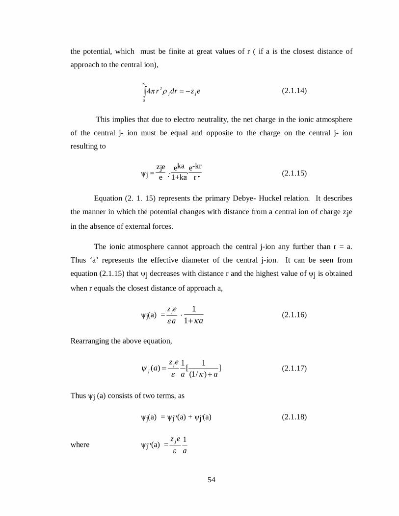
the potential, which must be finite at great values of r ( if a is the closest distance of

approach to the central ion),

24 j ja

r dr z e

(2.1.14)

This implies that due to electro neutrality, the net charge in the ionic atmosphere

of the central j- ion must be equal and opposite to the charge on the central j- ion

resulting to

ψj = zjee

eka1+ka

e-krr (2.1.15)

Equation (2. 1. 15) represents the primary Debye- Huckel relation. It describes

the manner in which the potential changes with distance from a central ion of charge zje

in the absence of external forces.

The ionic atmosphere cannot approach the central j-ion any further than r = a.

Thus ‘a’ represents the effective diameter of the central j-ion. It can be seen from

equation (2.1.15) that ψj decreases with distance r and the highest value of ψj is obtained

when r equals the closest distance of approach a,

ψj(a) = jz ea

1

1 a (2.1.16)

Rearranging the above equation,

1 1( ) [ ](1/ )

jj

z ea

a a

(2.1.17)

Thus ψj (a) consists of two terms, as

ψj(a) = ψj"(a) + ψj'(a) (2.1.18)

where ψj"(a) = 1jz ea

55

and ' ( ) [ ](1/ )

aj

j

z e eaa

The electrical potential due to an isolated charge q in a medium of dielectric

constant ε is given by

ψI = q/ε r (2.1.19)

Recalling that the charge of the central j- ion is zje and that of the ionic

atmosphere is –zje, it follows from above three equations that ψj"(a) represents the

electrical potential at r = a due to the central j-ion while ψj'(a) is the potential due to the

ionic atmosphere at r = (a + 1/κ). Thus the effect of the ionic atmosphere is equivalent to

the electric potential due to a charge –zje and distributed over a sphere of distance (a +

1/κ) from the central j-ion. The quantity 1/κ is called the thickness of the ionic

atmosphere. The parameter κ can be expressed in terms of the ionic strength (I) of an

electrolyte solution as

κ2 = 8πe2Nρ I/1000 εkt (2.1.20)

where I is defined as

212 i i

iI m z

The Gibbs free energy change of an aqueous ion, can be evaluated, from these

equations and can be given as

μje = - ka1

ke2

Nez 22j

(2.1.21)

This parameter is used to analyze the results in conjunction with the Bromley’s

model, and Lu and Maurer model discussed in the coming subtitles of the same chapter.

2. 1. 5: Inconsistencies in the D-H equation for the potential function and related

parameters that form the basis for this studies:

56

The approximations made to maneuver the mathematical hurdles, and to make the

approaches of evaluation naive leave several inconsistencies in the potential function

itself, and surprisingly, attempts are yet to be seen in the literature, to overcome this

lapse. To point out the main lapses, the following eight points are to be observed.

(1) The assumption that zieψj << kT is not too serious for points far from the central j-

ion, since in these regions, ψj should be small. However it involves errors in the

regions nearest to the j-ion at the origin.

(2) The linearization means that

ni' = ni (1 –zieyjkT ) (2.1.22)

which is referred as approximate distribution [17].

The quantity [ zieyjkT ] measures the ratio of the electrical energy of an ion to its

thermal energy, starting with this expression Bjerrum arrived at a very important

parameter called Bjerrum’s critical distance, “q”, an important parameter in connection

with ion-pair formation. It is given by Fuoss and Kraus using Bjerrum’s hypothesis [18]

as

21 2

2z z e

qkT

(2.1.23)

(3) Equation (2.1.15) fails to realize that the presence of the charged bodies in the

ionic atmosphere further entails the electric field and the dielectric constant of the

medium in the ion atmosphere or dielectric continuum. It becomes concentration

dependent, leading to a lowering with increment in the number of charged ions ,

added to the solvent . This aspect was theoretically studied by Glueckauff .

(4) Further observed that the total potential decreases monotonically with the distance

from the central ion. Since the assumptions of D- H premise that the ion- cloud

must be fine grained, expecting many ions within a distance (1/κ) from the central

57

ion. This makes the potential oscillate with increasing distance from the central

ion, instead of decreasing steadily throughout the cloud.

(5) The presence of the Potential function shown in equation (2.1.15) that it is not

uniquely defined with respect to position of the central ion because the effect due

to all the ions is incorporated . Hence for a given central ion (say J), if two more

different ions considered as central ions [say (J-1) and (J-2)], for a given fixed

volume element (dV) around them, the equation (2.1.15) may not define the

potential uniquely for them always.

(6) In the case of symmetrical single electrolyte systems, the approximations have

less limitations, under such conditions, z1 = -z2, n1 = n2 so that,

1 1 31 1 1 1

10 2 [ ] 0 [ ] .........3

j jj

z e z en z e n z e

kT kT

(2.1.24)

i.e., all terms in even powers vanish and therefore no errors of (zieψj/kT)2 etc. are

involved.

(7) Even though the model uses a distribution function for the ions on the basis of

Maxwell Boltzmann statistics, it was realized that, it was necessary to review the

distribution of the charge carriers, with an alternative distribution function.

(8) Several futile attempts for this model are available in literature by many authors,

most prominent of these are: Muller [19], Gronwall [20], Eigen and Wicke [21],

all of whom attempted to preserve the higher order terms to a greater extent, only

to lead to several complications.

Sengupta et.al., [22] used an intuitively deduced formula of Dutta and Bagchi

et.al, [23] which uses the formalism developed by Dutta [24]. This could increase the

range of calculation, but did not improve to any extent.

And also there are several parameters which influence the measurable

characteristics of electrolytic solutions which were not accounted in the electrolytic

theory of Debye-Huckle. They are:

58

1. The electrostatic short range interactions between ions of electrolyte, solvent Co-

sphere , and the cluster of ions and the single central ion.

2. The electro static field modifications are caused around any central ion which is

modified as the density of the increased charged ions and these results in a major

modification to the dielectric constant of the solvent continuum. Consequently all

the electrolytic state equations of different parameters are to be subjected to a

thorough modification, considering the lowering of dielectric constant of the

solution around the central ion.

2. 1. 6: Deviations from ideality:

The D-H theory deals with departures from ideality in electrolyte solutions [25,

26, and 27]. The main experimental evidence for this non- ideality is that:

1. Concentration equilibrium constants are variables.

2. Rate constants depend on concentration.

3. Molar conductivities for strong electrolytes vary with concentration.

4. Freezing points of electrolytes are different from what would be expected for

ideal behaviour.

These departures from ideality reduce as the concentration decreases and they

were attributed to the Columbic law of electrostatic interaction.

The activities of ions in solution are relatively large compared to neutral

compounds. Ions interact through a Columbic potential which varies as reciprocal of r,

where r is the distance between ions. Neutral solutes interact through London dispersion

forces that vary as r -6. The greater the charge on the ions, the larger the deviation from

ideality.

Pytkowicz et. al., proposed a partial long-range order model for aqueous

electrolyte solutions to avoid contradictions present in the Debye- Huckel theory. The

partial long-range order increases with increasing salt concentration because, as the ions

59

are closer together, the Columbic energy of interaction which generates, a quasi-lattice

increases. Furthermore, the order decreases with increasing temperature because the

thermal energy increases relative to the columbic attraction of the ions.

The net charge density ρj around a central ion j, according to the D-H Model can

be written as

( )2

( ) 4 1

jD raj

jD j

z e ea r

(2.1.25)

Where Zj is the valence of the ion at ‘j’, ‘ ’ is the electronic charge, is the reciprocal

of ionic atmosphere (which happens to be a function of the dielectric constant of the ionic

atmosphere), Da is the Debye radius and jr is the distance of the point under

consideration. Hence ( )j decreases monotonically from a maximum value at jr = Dai.e., the surface of the ion ‘j’, to zero.

The potential due to the effect of all the ions located in a volume element dV

in the solution situated at a distance jr from the central ‘j’ ion is not a unique function of

position, since the relative permittivity of the medium ε r, is responsible to control the

columbic interaction, between the charged entities. Consequently the depression in the

permittivity, with the concentration of the ionic system requires to be counted upon,

through the Glueckauff’s and Von Hippel’ s models. This observation was reported and

provided the necessary data, evaluated and experimentally established in this study.

2. 1. 7: Chemical Potential, Activity Coefficient, Gibbs free energy and Osmotic

Coefficient of an ion in solution:

(i) Chemical potential:

While studying the formation of ionic solutions, the most useful quantity [28] to

describe is chemical potential μi , defined as the partial molar Gibbs energy of the i th

component in a substance:

60

(2.1.26)

where xi can be any unit of concentration of the component: mole fraction, molality,

while for gases, µi is chemical potential which is a function of temperature T, pressure P

and mole fraction xi of the system, given as

lni i ikT a (2.1.27)

where ia is the activity by Lewis, designated by the symbol a . The activity gives an

indication of how active a substance is relative to its standard state as it provides a

measure of the difference between the substance’s chemical potential at the state of

interest and at its standard state. It depends on the composition. The standard state is

indicated by a superscript “δ”.

(ii) Activity coefficient:

In electrolyte solutions the activity coefficient is a measure of the deviation of the

idealized concentration {Aj} from the stoichiometric or analytical concentration, mj. An

activity coefficient is a factor used in thermodynamics to account for deviations from

ideal behavior in a mixture of chemical substances. This deviation is a result of the

electrostatic forces of attraction and repulsion which are present in electrolyte solutions.

A discussion of the concept of activity coefficient requires an analysis of the electrostatic

interactions in electrolyte solutions.

The activity coefficient ‘γi’ is defined as:

i i ia x ,

Reducing 2. 1. 27 as

lni i i ikT x (2.1.28)

61

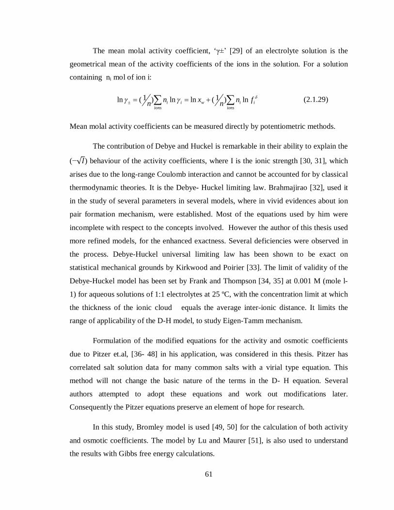
The mean molal activity coefficient, ‘γ±’ [29] of an electrolyte solution is the

geometrical mean of the activity coefficients of the ions in the solution. For a solution

containing ni mol of ion i:

1 1ln ( ) ln ln ( ) lni i w i iions ions

n x n fn n

(2.1.29)

Mean molal activity coefficients can be measured directly by potentiometric methods.

The contribution of Debye and Huckel is remarkable in their ability to explain the

(−√퐼) behaviour of the activity coefficients, where I is the ionic strength [30, 31], which

arises due to the long-range Coulomb interaction and cannot be accounted for by classical

thermodynamic theories. It is the Debye- Huckel limiting law. Brahmajirao [32], used it

in the study of several parameters in several models, where in vivid evidences about ion

pair formation mechanism, were established. Most of the equations used by him were

incomplete with respect to the concepts involved. However the author of this thesis used

more refined models, for the enhanced exactness. Several deficiencies were observed in

the process. Debye-Huckel universal limiting law has been shown to be exact on

statistical mechanical grounds by Kirkwood and Poirier [33]. The limit of validity of the

Debye-Huckel model has been set by Frank and Thompson [34, 35] at 0.001 M (mole l-

1) for aqueous solutions of 1:1 electrolytes at 25 ºC, with the concentration limit at which

the thickness of the ionic cloud equals the average inter-ionic distance. It limits the

range of applicability of the D-H model, to study Eigen-Tamm mechanism.

Formulation of the modified equations for the activity and osmotic coefficients

due to Pitzer et.al, [36- 48] in his application, was considered in this thesis. Pitzer has

correlated salt solution data for many common salts with a virial type equation. This

method will not change the basic nature of the terms in the D- H equation. Several

authors attempted to adopt these equations and work out modifications later.

Consequently the Pitzer equations preserve an element of hope for research.

In this study, Bromley model is used [49, 50] for the calculation of both activity

and osmotic coefficients. The model by Lu and Maurer [51], is also used to understand

the results with Gibbs free energy calculations.

62

(iii) Gibbs free energy:

The Gibbs potential measures the amount of work a system can do at constant

temperature (T) and pressure (P), given by:

G = U - TS + p V (2.1.30)

Hence Gibbs potential measures the amount of non-mechanical work a system

can do at constant pressure and temperature, or the amount of chemical work a system is

able to do [52].

The enthalpy measures the amount of work a system can do in an adiabatic,

isobaric process. This is the amount of non- mechanical work, since the pressure has to

be kept constant. Using Gibbs free enthalpy “G”, with standard convention, using the

standard definition of chemical potential [53]

i i i ii i

dG dN N d and

i ii

VdP SdT N d (2.1.31)

where Ni indicates the number of moles of the ith species.

Equations (2.1.31) are Gibbs- Duhem relations used to check the validity of the models.

The Gibbs free energy change which arises when an ion enters an electrolyte solution is

given by:

∆G = zje (∆j' -∆j") (2.1.32)

and can be positive or negative depending on the nature of the interactions between ions

and the solvent. This parameter is dependent upon the potential experienced by the

central ion itself, for a given concentration of the solute in the electrolyte system and that

governs all the mechanisms that come into existence, and is directly related to the

physiochemical consequences. The activity coefficient is related to the molar excess

Gibbs energy GE, by:

63

, ,ln [ ]j

Ei T P n

i

nGRT n (2.1.33)

In this equation, all the symbols have their conventional meaning. The excess

Gibbs energy of a solution is the difference between the actual Gibbs energy and the

Gibbs energy of the ideal solution at the same temperature T, pressure P and composition.

Anderko et.al [54], reviewed a large variety of models, in connection with Gibbs free

energy. Number of models with the D-H expression, like the UNIQUAC model [55] and

the NRTL models [56], using two different frame works, i.e., McMillan-Mayer (M-M)

framework, and Lewis- Randal (L-R) framework exist for the description of the excess

Gibbs energy of mixtures of molecular components. Some electrolyte models are

extended as models for the excess Gibbs energy calculation. Irrespective of the specific

model used to describe the individual thermodynamic properties as a function of factors

like concentration, temperature; it should be necessary that, the relationships between the

various functions must be thermodynamically consistent. Hence thermodynamic

parameter chosen for interpretation of the final result is to be evaluated with the

application of the fundamental definition of the same. In this thesis, Lu and Maure model

was used to calculate excess Gibbs energy values of chosen electrolytes from calculated

data of activity and osmotic coefficients from Pitzer model.

(iv) Osmotic coefficient:

In dilute aqueous solutions, the water activity and the water activity coefficient

are very close to unity. In order to report water activities without a large number of

significant digits, the osmotic coefficient is commonly used and is represented by the

symbol Φ, defined by Hammer and De Wane [57] as “an enhancement in the velocity of

the central ion, in the direction of the applied external field, as a result of more collisions

on the central ion from ions behind the central ion than from ions in front of it”. Jean

Vidal [58] gave a very detailed exposition about the thermodynamical aspects of osmotic

coefficient and its relation with several parameters.

64

2. 1. 8: Extended Debye-Huckel Equations and Debye-Huckel limiting law, for the

activity coefficient, and its limitations:

The basic concepts of D- H equation for the activity coefficient are given below.

The Debye- Huckel equation and Debye- Huckel limiting law were derived by Peter

Debye and Erich Huckel who developed a theory to calculate activity coefficients of

electrolyte solutions. Taking into account, the ion size parameter expressed in angstroms,

the original Debye- Huckel equation for the mean activity coefficient (γ), for a

completely dissociated binary electrolyte, consisting of ν ions (mole of solute)-1, with

charges Z +and Z -, Robinson and stokes [59] can be written as:

1 12 2

- ]log [ ] /[1Z Z A I aB I (2.1.34)

where I is the ionic strength in molality (m) units of concentration.

( / 2)I Z Z m , and Aγ and Bγ are parameters dependent on density and permittivity

of the solvent givenby,

2

3 3( )2 2

2 1( )1000 2.303 { }

N eAk T

in mole -1/2. I ½. (deg K)3/2 (2.1.35)

2 12

12

8 1{ } [ ]1000 ( )

NeBk T

in cm -1.mole -1/2I 1/2(deg K)1/2 (2.1.36)

For low values of I , the term [ 12aB I ], ultimately becomes negligibly smaller than

unity then

12

-log [ ]Z Z A I (2.1.37)

which is known as D-H Limiting law. The equation for the activity coefficient was

modified by K. S. Pitzer et. al.,. This model was most widely applied and reliable.

Several modifications were tried starting with the Pitzer’s model, to complement some of

the shortcomings of the assumptions of this model, and were tested by several authors. So

65

these tested equations of Pitzer model were used, for the calculation of activity

coefficient and osmotic coefficient to ensure the preliminary development over the

Debye- Huckel model, into which the dielectric constant variation was impregnated

suitably along with Bromley’s model.

2. 1. 9: Recent improvements over the Debye- Huckel equation: Pitzer model:

The activity is proportional to the concentration by a factor known as the activity

coefficient 훾, and takes into account the interaction energy of ions in the solution. It is

important to note that because the ions in the solution act together, the activity coefficient

obtained from the equation is actually a mean activity coefficient. The other approaches

based on this model are given by John Edwards [60], Maya B. Mane [61], Lloyd [62],

Bronsted [63], Guggenheim [64], Scatchard [65], McMillan Mayer [66], Chen et.al., [67-

72] and Krebs[73].

Detailed presentation of several models starting from lapses of Debye- Huckel

model are given by Horaico R Corti et.al., [74]. The electrolyte Non-Random Two-

Liquid model [75] (NRTL) is an activity coefficient model that correlates the activity

coefficients 훾 of a compound i with its mole fractions 푥 in the liquid phase concerned.

The concept of NRTL is based on the hypothesis of Hunenberger [76] that the local

concentration around a molecule is different from the bulk concentration. The NRTL

model of Chen et.al., combines a Debye- Huckel term with the NRTL local composition

model. The local composition concept is modified for ions, and the model parameters are

salt specific.The difference is due to a the interaction energy of the central molecule with

the molecules of its own kind Uii and that with the molecules of the other kind Uij. The

energy difference also introduces non-randomness at the local molecular level. The

NRTL model belongs to the so- called local- composition models. Other models of this

type are the Wilson model, the UNIQUAC model and the group contribution model

UNIFAC. These local composition models are not thermodynamically consistent due to

the assumption that the local composition around molecule ‘i’ is independent of the local

composition around molecule ‘j’. McDermott and Flemmer [77] established that this

assumption is not true.

66

McMillan and Mayer developed a theory starting from the virial equation of state.

Solutions of uncharged molecules can be treated by a modification of the McMillan-

Mayer theory. When a solution contains electrolytes, electrostatic interactions must also

be taken into account. The central ion surrounded by a spherical cloud that is made up of

ions of the opposite charge is used and expressions were derived for the variation of

single-ion activity coefficients as a function of ionic strength. Debye- Huckel theory

takes no account of the specific properties of ions such as size or shape.

Later, other types of models have been developed to extend the Debye- Huckel

law to higher concentrations [78]. The first extension was to impose a restriction for a

closest approach distance to ions as the ions in the cloud could not approach the central

ion by more than some distance.

Earlier to the Debye- Huckel theory, Brønsted had independently proposed

empirical equations for activity and osmotic coefficients where the activity coefficient

depended not only on ionic strength, but also on the concentration, m, of the specific ion

through the parameter β.

Activity Coefficient: lnγ = −αm1/2– 2βm

Osmotic Coefficient: 1 –φ = (α/3) m1/2 + βm

This is the basis of SIT theory, used to estimate single- ion activity coefficients in

electrolyte solutions at relatively high concentrations, by taking into consideration

interaction coefficients between the various ions present in solution. Interaction

coefficients are determined from equilibrium constant values obtained with solutions at

various ionic strengths. The determination of SIT interaction coefficients also yields the

value of the equilibrium constant at infinite dilution.

Guggenheim and Scatchard extended the theory to allow the interaction

coefficients to vary with ionic strength. Bromley model, the Pitzer model, were

developments from this models. Pitzer’s model took the expressions of the osmotic

coefficient obtained from the extended Debye-Huckel law and applied a virial expansion

in molality, as suggested by other theories.

67

The success of the Pitzer model lies in the fact that it opens the way to the

description of highly concentrated solutions, up to 6 or 10 mol/kg, with a few parameters.

However it was observed by many authors (mainly Guggenheim and Turgeon) that the

Pitzer’s model fails to recognise substantial major discrepancies that encounter even at

concentrations greater than 0.1 mol/kg. It fails to reveal intricate aspects of happenings at

lower concentrations than the above successful range of concentrations because of the

apparent crudeness in assumptions. At lower concentrations, the results reported even

with D- H model of electrolytic solutions would probably get masked because of the

nature of virial terms of expansion and the approximations during their application. It

curtails to reveal ions of finer traits involved in some of the interactions attempted for

study, and hence the outcome of the application of this model cannot be comprehensive.

It is to be realised that due to these conspicuous drawbacks, even the similar models like

the Bromley’s model, cannot deliver the expected improvements, leading to non-

comprehensive outcomes. The apparent inherent short comings traced by the author, are

detailed in the article 2.1.11, of this chapter. Nevertheless, the Pitzer’s parameters have

limited physical meaning, since the virial expansion was empirically introduced in the

model. It retains the basic physical concepts involved in the D- H model, to explain the

mechanisms involved.

Another method of investigation has also been explored by using the statistical

mechanics to obtain thermodynamic quantities for ionic solutions and it has been carried

out with the help of the Ornstein- Zernicke (OZ) equation and by treating the solution in

the McMillan Mayer formalism. The OZ equation treats statistically the interactions

between particles by taking Pitzer’s model. As it is the best of the earlier models, it was

chosen for application of the earlier published dielectric data in the present study.

Thomsen [79] developed equations for multi-phase flash calculations required for

aqueous electrolyte process simulations in his doctoral work and multiple steady states

were detected and analysed. Their equations are essentially similar to those of Nicolaisen

et.al., [80]. They pointed out that in order to apply the Debye- Huckel theory, to non-ideal

systems; it has to be primarily combined with a term for short-range interactions.

68

Thomsen et. al., developed the extended UNIQUAC model in which the Debye- Huckel

contribution to the excess Gibbs energy was deduced.

Pessôa Filho et.al., [81] observed that mixtures containing compounds that

undergo hydrogen bonding show large deviations from ideal behaviour. These deviations

can be accounted for chemical theory, proposed by Dolezalek [82] according to which the

formation of a hydrogen bond can be treated as a chemical reaction. This chemical

equilibrium needs to be taken into account when applying stability criteria and carrying

out phase equilibrium calculations. They illustrated the application of the stability criteria

to establish the conditions under which a liquid- phase split may occur and the

subsequent calculation of liquid- liquid equilibrium using Flory- Huggins equation

modified by a chemical- theory to describe the non- ideality of aqueous two-phase

systems composed of poly ethylene glycol and dextran. The model was found to be able

to correlate ternary liquid-liquid diagrams reasonably well by simple adjustment of the

polymer-polymer binary interaction parameter. Chemical theory to modify excess Gibbs

energy models began with Kretschmer and Richard Wiebe [83], who used this theory to

modify the Flory- Huggins equation [84, 85]. During l970’s, Waisman and Lebowitz

[86] solved the MSA for the restricted primitive model. A rapid succession of new results

on more sophisticated models of ionic solutions was developed. The MSA equations have

been solved for asymmetrical ions, mixtures of charged hard spheres and dipolar spheres,

and charged particles near a wall. The MSA itself has been improved in many ways by

the techniques of cluster resumptions [87]. This work was later supplemented and

arranged in a more complete form by Renon and Prausnitz [88], Nagata and Kawamura

[89], Nagata [90], Nath and Bender [91, 92], Brandani [93] and Evangelista [94]. They

have also used chemical theory to modify the UNIQUAC equation of Abrams and

Prausnitz et.al., [95], the parameters and various thermodynamic properties necessary for

performing calculations with the extended UNIQUAC model and published in a number

of papers [96- 102]. The main difference between these models lies in the way the

chemical equilibrium between clusters formed through hydrogen bonding is calculated.

69

2. 1. 10: Omissions in Pitzer model:

The Pitzer model was developed as an improvement upon earlier model

proposed by Guggenheim, involving some approximations about the concentration limit

in connection with the osmotic coefficient of a reference salt which worked well at low

electrolyte concentrations [103], but contained discrepancies at higher concentrations

(>0.1M). Scatchard suggested some modifications to these concepts, to provide a

compact summary of the experimental data but failed to cater to the desired requirements.

On the basis of the insight provided by the improvements of Friedman and

collaborators [104], Card and Valleau [105], the Pitzer model came to light and attempted

to resolve these discrepancies, without resorting to excessive arrays of higher- order

terms. Pitzer used AΦ, called the Debye- Huckel term, for simplification of the equations

applicable to 2- 2 electrolytes. The equations of Pitzer used in the present study are given

hereunder.

In the Pitzer model, the activity coefficient of each ion is described by two terms.

The first one is due to long-range interactions (electrostatic or Debye- Huckel behaviour)

given by f , the second one is due to short-range interactions which are expressed in

terms of second and third coefficients of a virial equation [106].

Pitzer stated that, some marked omissions are inherent in his model. They are

1: The model starts with the system proposed by Guggenheim which follows the

principle of Specific interaction of Bronsted, excluded terms related to short range

forces between the like sign ions which is fairly inaccurate when we want to

consider the electrostatic contributions for the evaluation of depression in the

dielectric constant, as conceived in the Glueckauff’s model. A similar line of

thought is continued in Pitzer’ s model which throws its impact on the final results

of findings reported in this thesis because mechanisms like the ion-pairing, polar

interactions etc. need cognizance.

2: The virial coefficients used in the equations are from the experimental origin;

their statistical method of evaluation would not consider the ionic level

70

happenings and their dependence on intricate properties like the relative

permittivity on the concentration of the electrolyte in the solvent. Consequently

the mechanisms that take place within ionic atmosphere during solvation and also

the solute- solvent interactions are not accounted in the statistical methods

involved for the virial coefficients of the Pitzer’s model.

3: Two assumptions about phenomena and concepts are erroneous. They are:

(i) The direct interactions of solute species at short distances and changes in

solvation with concentration which influence the effective inter ionic potential of

average force are not distinguished,

(ii) The distinction between molality and concentration is ‘ignored’, because mainly

the statistical calculations are used, based upon the molecular models, to develop

empirical form of qualitative understanding. Especially molality is preferred by

Pitzer since he presumes that the temperature variations influence the activity

and osmotic coefficient to a lesser extent with molality.

However happenings around the proximity of the ion in the co- sphere are not

compatible with these approximations, as the ion-pair formation around the central ion is

sensitive to even the least potential contribution either in the proximity or at a reasonable

distance from the site of mechanism.

4: Guggenheim and Turgeon pointed out that substantial discrepancies arise even at

concentrations greater than 0.1mol/kg. Several authors made variety of attempts

to accommodate this, but to no avail [107]. Scatchard and his co-workers [108]

extended and elaborated Guggenheim equations in several ways. First they

subdivided the Debye- Huckel term in the expression for excess Gibbs Energy

into a series of terms with different coefficients of I 1/2 in ‘r’ corresponding to

different distances of closest approach for the solute components .

5: Appropriate derivatives later yield complex formulae for the coefficients γ and φ.

Bronsted’ s principle of Specific interaction is abandoned and terms are

introduced for the short range interaction of ions of like sign. Arrays of third and

71

fourth virial coefficients are added by Lietzke and Stoughton [109]. The osmotic

coefficient data for 20 pure electrolytes was represented by them to a fair

accuracy. Several systems of mixed electrolytes were treated also, resulting in a

system of equations is unwieldy and raises other complications, because the

physical interpretation of the involved terms and parameters become complex.

These omissions during the development of the theoretical equations of the model

were attempted in a pragmatic way, by making the equations simpler with more

meaningful parameters introduced in the Pitzer’s work.

The fundamental deficiency in the basic Debye- Huckel theory is the recognition

of the parameter the distance of closest approach, ‘a’ in the calculation of the electrostatic

energy in the distribution of ions. However the kinetic effect of hard core on γ and φ is

ignored. Kirkwood points out that the hard-core effects cannot be treated rigorously in the

traditional way, by calculating the free energy. Terms were added by Rysselberghe and

Eisenbergto[110] improve hard core effects, only for the feature of the particular interest

to be lost. Sengupta, Bagchi and Dutta attempted the application of new statistics and

developed a new set of distribution equations. Dutta and Bagchi deduced theoretically

,

1 1rz kTr e

bn

(2.1.38)

where , rn : the number density of positive or negative ions,

b : the volume of the covering spheres of positive or negative ions ,

: parameters of distribution, z valence of the positive or negative ions and

ε , k and T have their usual significance.

The formalism used in this equation has been developed by Dutta and Bagchi, and

rests on the assumption that ions having characteristic volume of their own are under the

influence of their mutual electrostatic field in solution. Eigen and Wicke used a similar

72

distribution formula in their theory of strong electrolytes in a different form with slightly

different explanation for the parameters involved.

Sengupta et.al, evaluated the available electric energy, through the evaluation of λ

where kT

. The Poisson-Boltzmann equation was then solved. An expression for

the Activity coefficient was then deduced using separate ionic radii for the ions.

Hill [111] using Statistical mechanics proposed a convenient equation for hard

core potential and was used in the Pitzer’s model for the osmotic coefficient. However

the equations of the statistical origin involve errors in the qualitative as well as

quantitative observations. This is to be accommodated at some juncture to make the

Pitzer’s model better. Attempts of other workers in literature are not concentrating on

these aspects. Consequently there will be marked deviations between the results of the

application of the present theories and experimental findings. The explanation of the

mechanisms like Eigen and Tamm Ion pair formation leave dissonance between theory

and experiment as is found in some results in the present study, discussed in the chapter

results and discussion. The application of Pitzer model, to the dielectric data obtained

using a very accurate operational amplifier technique is presented below.

2. 1. 11: Pitzer’s retention of the " "A or slope of Debye-Huckel limiting law:

The Pitzer’s model uses primarily the concepts of the Debye- Huckel model. An

important parameter that appears in the Pitzer model is A called the Debye-Huckel term,

given by

32 2

0213 1000

dN eAkT

(2.1.39)

(Terms are explained in article:4.2.2) This is the Debye- Huckel limiting law

slopes from the basic equation of the osmotic coefficient and is a function of temperature

given by a polynomial correlation in ‘T’, used by Morteza Baghalha [112], taken from

Archer and Wang [113). This parameter was obtained from a careful evaluation of

73

density and dielectric constant data by Pitzer, Royf Sylvester , Holmes and Mesmer

[114]. Debye and Huckel originally coined this parameter, and were later modified by a

host of workers, considering the very accurate experimental data from more than one

source which gives a comprehensive picture about the ion pair formation mechanism that

will be discussed later.

2. 1. 12: The Pitzer equations for activity coefficient and osmotic coefficient:

Pitzer started with the fundamental quantity of excess Gibbs free energy and

begins with a virial expansion. Further, the free energy is expressed the sum of chemical

potentials, or partial molal free energy, and an expression for the activity coefficient is

obtained by differentiating the virial expansion with respect to molality.

For a simple electrolyte MpXq, at a concentration m, made up of ions Mz+ and Xz−,

the parameters f , MXB and MXC are defined by

( ' )

2

ffIf

(2.1.40)

' ( ){ ' } ( ){ ' }2 2MX MX MX MM MM XX XXp qB I I Iq p

(2.1.41)

3{ }( )MX MMX MXXC p qpq

(2.1.42)

The B parameter was found empirically to show an ionic strength, I dependence

(in the absence of ion-pairing) which could be expressed as

(0) (1) IMX MX MXB e (2.1.43)

For 2-2 electrolytes, activity coefficient γ given by Pitzer and Mayorga [41] as,

2ln 4 MX MXf mB m C (2.1.44)

74

Where 1/2 1/2 1/2

0[ / ( ) (2/ )ln(1 )]f A I I bI b I bI and I = 1/2 ∑mz2

1/ 21

1/ 22

2

2 2(0) (1) 1/ 21 1 1

2 2(1) 1/ 22 2

12 (2 )[1 ( ) ]2

1(2 )[1 ( ) ]2

IMX MX MX

IMX

B I I I I e

I I I I e

And

(3/ 2)MX MXC C ,3

2 2021

3 1000dN eA

kT

Osmotic coefficient ф is given by

Ф-1 =4fф+mBфMX+m2Cф

MX (2.1.45)

Where 1 12 2[ /(1 ) ]f A I bI

And 1 12 2

1 20 (1) (2)I IMX MX MX MXB e e

Similarly for (2-1), (3-1) Electrolytes,

lnγ = |zMzX| f γ+ m M X2

MXB

+ m2 3/2M X2

MXC

(2.1.46)

in which νM and νX are the numbers of the M and X ions in the formula and also

ν = νM +νX, and zM and zX give their respective charges in electronic units and

ф -1= |zMzX| f ф+ m M X2

MXфB + m2 3/2

M X2

MXфC (2.1.47)

2. 1. 13: ‘B, α and β’ relations used in the model:

Pitzer used a set of virial coefficients 0 1, ,B and 2 which can be expressed

in the form of an equation

1 1

2 21 20 1 2I IB e e

75

where (0) and (1) represent the effect of short range forces. (2) and 2

correspond to the anomalous behavior of the 2-2 electrolytes. The parameters 1 and 2

are assigned with a series of values by Pitzer et.al. The values of these coefficients are

obtained by Pitzer, from experimental data statistically, and are available in literature.

Besides the set of parameters obtained by Pitzer et. al., in 1970s, Kim [115] and

Frederick [116] published the Pitzer parameters for 304 single salts in aqueous solutions

at 298.15 K, extended the model to the concentration range up to the saturation point.

Those parameters are widely used for many complex electrolytes including organic

anions or cations, which are very significant in some related fields, were not summarized

in their paper.

In the original notation used by Pitzer et.al., all the parameters that are adjusted

for each electrolyte are given in the subscript MX. The symbols γ, (1), and (0) etc are

labels but not exponents, and b = 1.20, assumed by Pitzer (1973), in his original paper.

The data for the four parameters β(0) , β(1), β(2), and Cγ were fitted by least squares

adjustment, 1 =1.4 and 2 = 12.0 was used in all the calculations of this Thesis. The

values of these parameters used in the calculations are given in Table: 4.2.1

These equations were applied by Pitzer et.al, with minor suitable modifications to

an extensive range of experimental data at 25 °C with excellent agreement to about 6 mol

kg−1 for various types of electrolytes. The treatment can be extended to mixed

electrolytes and to include association equilibria. Values for the parameters β(0), β(1) and

C for inorganic and organic acids, bases and salts have been tabulated. Temperature and

pressure variation is also discussed at appropriate places by them.

In these Equations, the BMX term corrects for ion-ion interactions, whereas the

CMXterm corrects for ion- ion- ion interactions. Pitzer et. al., have obtained values of

β(o), β(1) and Cф for several electrolytes and obtained good agreement with

experimental data (up to 6M) when the assumption is made that for all electrolytes, α =

2.0 and b = 1.2. The Cф values are generally small, which means that in most cases, CMX

can be ignored.

76

2. 1. 14:The Bromley Model:

Friedman [117] deduced a set of equations for conversion between two frame

works of Lewis- Randall and McMillan-Mayer for the thermodynamic excess functions

of solutions. Several inconsistencies came to lime light. Martin Breil [118] finds that the

Friedman's equations only are valid for dilute solutions makes his results limited and not

generally applicable.

A generalized analytic correlation is presented for activity coefficient, osmotic

coefficient, enthalpy, and heat capacity of single and multi- component strong aqueous

solutions, by Bromley who showed that it is possible to assign individual values of β to

ions i.e;

βMX = βM+ βX (2.1.48)

Bromley’s one parameter model is much easier to use than Pitzer’ s three-

parameter equation even though the latter is established in this thesis to be more accurate

in many ways, by virtue of the fact that the Pitzer treatment is more comprehensive.

Bromley pointed out that his method does not perform satisfactorily for divalent metal

sulphates, sulfuric acid and zinc and cadmium halides. These electrolytes are all partially

associated in solution. It is this association which makes it difficult to estimate γ12 values

by a model, since this equation does not take the degree of dissociation into account. The

true ionic strength will depend on the association equilibrium and it would nevertheless

be more convenient, if a way could be found to estimate activity coefficients using the

stoichiometric or apparent ionic strengths. Pitzer and Mayorga have presented such a

model for 2- 2 electrolytes. Basically, they used their earlier equations. Bromley’s

equations of the “one parameter” model: originate from the activity coefficient equation

1 2

121 1 2

122

(0.06 0.6 )log 1.5(1 )1

z zA Z Z I B I BI

Z ZII Z Z

(2.1.49)

Bromley, [49, 50] presented values of B for 1- 1, 1- 2, 1- 3, 2- 1, 2- 2, 3- 1, 3-2

and 4-1 electrolytes which predict upto I = 6 with a maximum error not exceeding

77

5%. The B values are in the range -0.50 < B < 0.25. And for an electrolyte they can be

estimated with the equation,

B = B+ + B- + δ+ δ- (2.1.50)

The values of B for chosen electrolytes were given in table 4.2.1. Starting with above

equation, it is possible to write equations for a number of other thermodynamic properties

using rigorous thermodynamics. The resulting equation for osmotic coefficient is given

by

11221 2.303 ( ) 2.303(0.06 0.6 ) ( )

3 2I IA z z I B Z Z aI 2.303

2IB

(2.1.51)

where, Aγ is Debye- Huckle coefficient, given by 3Aф and

1.0 , 1.5a

Z Z

, 1 1 12 2 2

1 132 2

3 1( ) [1 2ln(1 )( ) [1 ]

I I II I

’

2

2 1 2 ln(1 )( ) [ ](1 )

aI aIaIaI aI aI

2. 1. 15: Electro negativity model of Keyan Li et. al., :

Keyan Li et. al., [119], proposed a model taking electro negativity scale into

consideration. Incorporating the solvent effect into the Born effective radius, they

proposed an electro negativity scale of metal ions in aqueous solution with the most

common oxidation states and hydration coordination numbers in terms of the effective

ionic electrostatic potential. They concluded that the metal ions in aqueous solution are

poorer electron acceptors compared to those in the gas phase. It is interesting to note that

the frame work of D-H Model is retained even in this model. They claim that this

solution-phase electro negativity scale showed its efficiency in predicting some important

properties of metal ions in aqueous solution such as the aqueous acidities of the metal

ions, the stability constants of metal complexes, and the solubility product constants of

the metal hydroxides. They elaborated that the standard reduction potential and the

78

solution-phase electro negativity are two different quantities for describing the processes

of metal ions in aqueous solution to soak up electrons with different final states. This

work provides a new insight into the chemical behaviours of the metal ions in aqueous

solution, indicating a potential application of this electro negativity scale to the design of

solution reactions. It intends to study and apply this model, in the future extension work

with experimental studies using suitable technique.

Fig: 2.1.3 Electro negativity model developed by Keyan Li et, al, (2012).

2.1.16: Lu and Maurer model:

During 1993, Xiaohua Lu and Maurer [120] published a model for the excess

Gibbs energy GE of aqueous solutions containing mixed electrolytes. This was extended

[121] from temperatures 298 K to temperatures up to 573 K in 1996. The extension is

achieved by introducing a universal relation for the influence of temperature on some

model parameters. Although parameters are still ion specific, the influence of temperature

on those parameters is universal. No additional parameters are required for describing

aqueous solutions of mixed electrolytes. The model accurately predicts activity

coefficients at high temperatures and at concentrations up to the solubility limit in

electrolyte aqueous solutions containing, K+, Na+, NH4+ ,(SO4 )2-,Cl- and NO3

- .

79

The model is to describe the excess Gibbs energy and related properties like

osmotic coefficient and mean activity coefficients of dissolved electrolytes in aqueous

solution.

It is assumed that dissolving strong electrolytes in water results in a mixture of

water molecules, unsolvated and solvated ions. Solvation equilibria are used to calculate

the true concentrations of solvated and unsolvated ions from the overall concentrations of

the dissolved electrolytes. Physical interactions between all species are taken into account

by combining the Debye- Huckel law with the UNIQUAC model of Abrams and

Prausnitz [122]. The emperical temperature dependence of this model was carefully

tested by the prediction of excess enthalpy, with the Gibbs-Helmholtz relation.This

model describes excess Gibbs energy and related properties. However the deppression in

the dielectric constant of the dielectric continuum of the solvent on the dissolution of the

electrolyte does not figure in the calculations, of Lu and Maurer. Application of

experimental data in this study, for this lowering of dielectric constant to (1) the Bromley

model (2) Lu and Maurer model for evaluation of activity coefficient and osmotic

coefficient, and later evaluation of Gibbs free energy, gave inconsistant results, that

would be discussed in the chapter ‘ Results and Discussion’. However concrete evidence

of the ion pair formation expected by Eigen and Tamm mechanism, was traced with the

Pitzer’s model to a greater extent.

The Excess Gibbs energy of the solution was evaluated in this thesis using the

notation of Lu et.al. , in terms of osmotic coefficient ф and activity coefficient 훾∓ .The

relationship can be expressed as:

(1 ln )EwG n mRT (2.1.52)

where nw is mole number of water and the remaing terms have their usual notation.

The relative enthalpy is related to EG by

2,

/[ ]E

P mG TL T

T

(2.1.53)

80

The Apparent Relative Molar Enthalpy that requires experimental data is given by

2,

ln[( ) ( ) ]P mw

LL RTn m T T

(2.1.54)

In all the above equations, the notation of Prigogine and Defay and Xiaohua Lu and

Maurer was used.

2.2. Dielectric Study:

Attention was focussed on Glueckauff’ s model in this thesis, and evaluated the

dielectric data using this model. An apparatus, using latest operational amplifier circuitry,

was designed and fabricated for the accurate dielectric measurements to obtain the data of

the lowering of dielectric constant of chosen aqueous electrolytic solutions. This

experimental data showed an excellent agreement with the experimental, theoretical

computation of the variation of the dielectric constant using Glueckauff’ s model. The

author of this thesis used the equations and applied his experimental dielectric data for

the relevant parameters from the several electrolytic models developed by Pitzer,

Bromley, Lu and Maurer, to evaluate chain of thermodynamic parameters like activity

coefficient, osmotic coefficient and excess Gibbs energy. The details of the present set up

are given in the chapter ‘Experimental Techniques’. However the frequency

determination was also not reasonably accurate in the dielectric constant determination.

The researchers reported the usage of an electronic network made up of vacuum tube

circuits then and even the frequency determination is better and improved now. The

experimental dielectric , acoustic and thermodynamic data for the short range as well as

long range interactions not only revealed valuable information about ion pair formation,

which is the Noble prize winning hypothesis of Manfred Eigen and Tamm for the year

1967 [123] but also in a position to provide valuable leads, for the dissemination of the

information.

81

2. 2. 1: Glueckauff’s Dielectric model, and Lowering of Dielectric Constant of the

Solvent on addition of Solute:

A careful observation of the equations for the ‘ψ’, and ‘κ’ obtained above, reveals

that a big lapse has occurred in the development of the Debye- Huckel model. It is the

electrostatic influence of the ions of the solute (carrying charge), on the electric field

caused at the central ion, with respect to the electrostatic permittivity of the dielectric

continuum of the solvent surrounding the central ion and incorporating the ionic

atmosphere. Various other attempts for the modification of the D- H model would result

in a half- hearted approach unless we take regard of this main lapse. This was done by

Glueckauff in his model for the depression in the permittivity of the solvent to which

solute ions are added.

Robinson Wright [124], Robinson and Stokes, Falkenhagen, and Harnedand

observed that the internal field around the central ion of the ionic atmosphere created by

the charged solute ions in the solvent of the electrolytic solution tend to reduce the value

of the dielectric constant of the electrolytic solution. This aspect is overlooked and the

departures exhibited in the properties of electrolytic solutions, as the concentration

increases, cannot be satisfactorily explained, by the Debye- Huckel model (adopting the

idea of self-consistent field) even with its several recent modifications proposed by a host

of workers with this objective. It was pointed out by Hasted, Ritson and Collie [125, 126]

that a variation of dielectric constant would have a significant, if not dominating, effect

on the properties of concentrated salt solutions. Further, Sack made a theoretical estimate

of the lowering of dielectric constant that would be expected due to the saturation of the

dielectric in the neighbourhood of an ion. Both these studies are of great theoretical

interest. They made dielectric measurements with more than one method at microwave

frequencies. Wolynes observed that the earlier accurate experimental data on

measurements of electrical conductivity and electric potential, and other related data on

several interesting phenomena became a point of interest and many a time a discrete

controversy. The long range ion- ion interactions could be used to arrive at the limiting

theoretical results that showed an agreement with experiment.

82

Wang and Anderko [127], developed a general model for calculating the dielectric

constant of mixed solvent electrolyte solutions, by the empirical modification of

Kirkwood theory for multi- component systems. A simple relationship between dielectric

constant of mixed solvents with solvent composition and temperature was proposed by

Abolghasem Jouyban et.al., [128].

Wear [129] reported for pure liquids a technique for relative permittivity

determination. The Sargent oscillometer technique is good enough but not compatible for

temperature controlled measurements. Even though this method is a development for the

oscillometer method, its accuracy of measurement of temperature is restricted, mainly

because a temperature bath is used to regulate the temperature by a liquid circulation

technique. Till now the dielectric properties of the ion conducting systems have not been

examined, despite their fundamental importance. Chemists are keen to obtain information

on the structure of solutions which can be provided by permittivity measurements.

Theoreticians hope to get more insight into the dynamic and transport properties of

electrolyte solutions from knowledge of relaxation times and dielectric decrements.

Theoretically [130] the equation for the temperature dependence of relative permittivity

is given as,

휀 = (휀 ) 푒 (2.2.1)

where ε is the dielectric constant , T is the absolute temperature , and L and ε0 are

constants for a given solvent .The theoretical value of ε has been evaluated using this

equation.

A similar method was [131] used for the water- ethanol system also. The water-

methanol data of Wear recorded discrete departure between theory and experiment .This

is expected, as per the observations of other prominent findings of different [132-134]

techniques, like U-V visible spectro- photometry, ion selective electrode potentiometry,

dielectric relaxation spectroscopy and titration calorimetry.

Von Hippel [135] and others [136, 137] showed that the dielectric constant in the

vicinity of the central ion is modified by the volume fraction of the ions in layer of the

solvent around the central ion. Glueckauff deduced an expression for the lowering of the

83

dielectric constant of the solvent when a solute is added to it, on the basis of

thermodynamic and electrostatic expressions given by Booth [138].

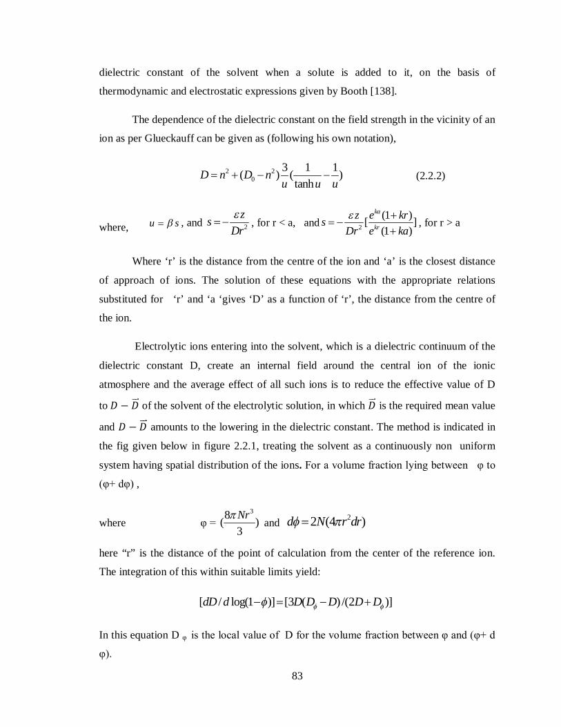
The dependence of the dielectric constant on the field strength in the vicinity of an

ion as per Glueckauff can be given as (following his own notation),

2 20

3 1 1( ) ( )tanh

D n D nu u u

(2.2.2)

where, u s , and 2

zsDr

, for r < a, and 2

(1 )[ ](1 )

ka

krz e krs

Dr e ka

, for r > a

Where ‘r’ is the distance from the centre of the ion and ‘a’ is the closest distance

of approach of ions. The solution of these equations with the appropriate relations

substituted for ‘r’ and ‘a ‘gives ‘D’ as a function of ‘r’, the distance from the centre of

the ion.

Electrolytic ions entering into the solvent, which is a dielectric continuum of the

dielectric constant D, create an internal field around the central ion of the ionic

atmosphere and the average effect of all such ions is to reduce the effective value of D

to 퐷 − 퐷⃑ of the solvent of the electrolytic solution, in which 퐷⃑ is the required mean value

and 퐷 − 퐷⃑ amounts to the lowering in the dielectric constant. The method is indicated in

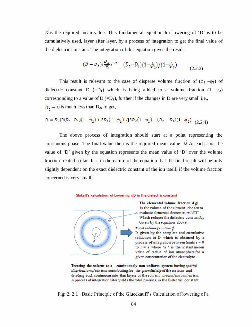
the fig given below in figure 2.2.1, treating the solvent as a continuously non uniform

system having spatial distribution of the ions. For a volume fraction lying between φ to

(φ+ dφ) ,

where φ = 38( )

3Nr

and 22 (4 )d N r dr

here “r” is the distance of the point of calculation from the center of the reference ion.

The integration of this within suitable limits yield:

[ / log(1 )] [3 ( ) /(2 )]dD d D D D D D

In this equation D φ is the local value of D for the volume fraction between φ and (φ+ d

φ).

84

is the required mean value. This fundamental equation for lowering of ‘D’ is to be

cumulatively used, layer after layer, by a process of integration to get the final value of

the dielectric constant. The integration of this equation gives the result

= (2.2.3)

This result is relevant to the case of disperse volume fraction of (φ2 –φ1) of

dielectric constant D (=D1) which is being added to a volume fraction (1- φ2)

corresponding to a value of D (=D2), further if the changes in D are very small i.e.,

is much less than D2, to get,

(2.2.4)

The above process of integration should start at a point representing the

continuous phase. The final value then is the required mean value . At each spot the

value of ‘D’ given by the equation represents the mean value of ‘D’ over the volume

fraction treated so far .It is in the nature of the equation that the final result will be only

slightly dependent on the exact dielectric constant of the ion itself, if the volume fraction

concerned is very small.

Fig: 2. 2.1 : Basic Principle of the Glueckauff’s Calculation of lowering of εr

85

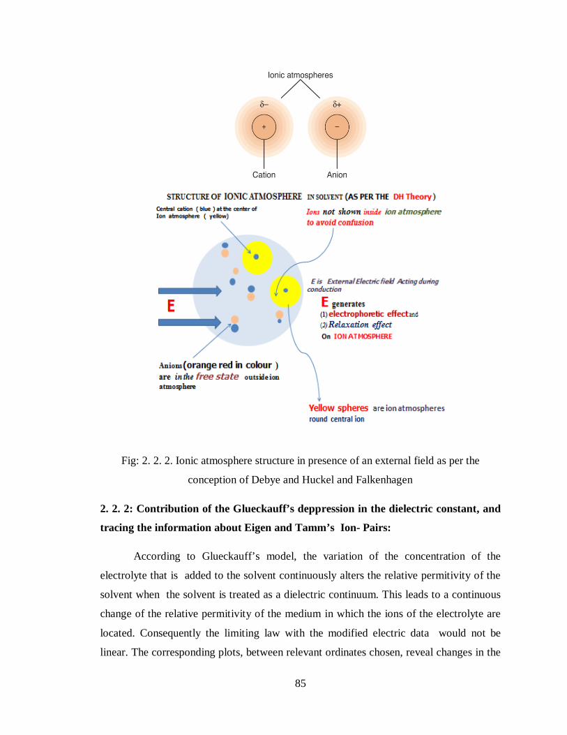
Fig: 2. 2. 2. Ionic atmosphere structure in presence of an external field as per the

conception of Debye and Huckel and Falkenhagen

2. 2. 2: Contribution of the Glueckauff’s deppression in the dielectric constant, and

tracing the information about Eigen and Tamm’s Ion- Pairs:

According to Glueckauff’s model, the variation of the concentration of the

electrolyte that is added to the solvent continuously alters the relative permitivity of the

solvent when the solvent is treated as a dielectric continuum. This leads to a continuous

change of the relative permitivity of the medium in which the ions of the electrolyte are

located. Consequently the limiting law with the modified electric data would not be

linear. The corresponding plots, between relevant ordinates chosen, reveal changes in the

86

gradients, significant of the three types of the ion pairs envisaged by Eigen and Tamm

mechanism. Aγ and Bγ are the two important locations of the basic D- H equations,

involving the impregnation of the variation of the dielectric constant data given in this

thesis, where information about the Eigen and Tomm mechanism is obtained.

2.3: Eigen and Tamm’s Ion pair Mechanism Study [ETIPM]:

The mechanism has been established on vigorous experimental data, obtained by

several workers. However the fundamental concept of ion pairs has the origin from the

basic Coulomb interaction. Hence the dielectric continuum is responsible to organize the

ion solvent interactions and the successive stages of the mechanism as envisaged from

the fundamental concepts and the equation developed by Bjerrum. Ions of opposite

charge are naturally attracted to each other by the electrostatic force given by coulomb’s

law. The most important factor to determine the extent of ion- association is the dielectric

constant of the solvent. The concept has been worked out earlier by Bjerrum, and by

other authors including Fuoss et.al., all of whom failed to realise the findings of

Glueckauff. Eigen and Tamm proposed the Ion Pair Formation Mechanism. Eigen [123]

was awarded Nobel Prize in Chemistry for the year 1967 for the study of fast ionic

reactions along with Leo de Maeyer using nanosecond ultrasound absorption and thermal

conductivity techniques and was the first to bring out the existence of the mechanism on

rigorous experimental basis. Generally ion- pairs are formed when a cation and an anion

come together. Details of the mechanism will be explained in the chapter ‘Results and

Discussions’, under the article: 4.2.1.

Presently, three distinct types of ion- pairs on the basis of solvation of the two

ions are recognized. The mechanism can be broadly viewed as a three step process, fig: 2.

3. 1. For the purpose of this presentation, secondary solvation is ignored. When both ions

have a complete primary solvation sphere, the ion-pair may be termed as ‘fully solvated’

or solvent- separated. When there is one solvent molecule between cation and anion, the

ion-pair may be termed as ‘solvent- shared’. Finally when the ions are in contact with

each other the ion-pair is termed a ‘contact ion- pair’. Even in a contact ion- pair, the ions

retain most of their solvation shell. The nature of this solvation shell is generally not

known with any certainty. In aqueous solutions and in other donor solvents, metal cations

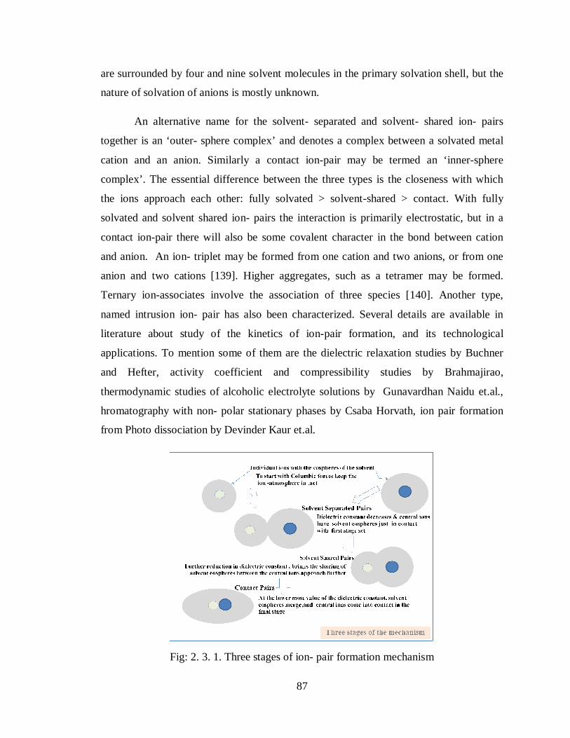
87

are surrounded by four and nine solvent molecules in the primary solvation shell, but the

nature of solvation of anions is mostly unknown.

An alternative name for the solvent- separated and solvent- shared ion- pairs

together is an ‘outer- sphere complex’ and denotes a complex between a solvated metal

cation and an anion. Similarly a contact ion-pair may be termed an ‘inner-sphere

complex’. The essential difference between the three types is the closeness with which

the ions approach each other: fully solvated > solvent-shared > contact. With fully

solvated and solvent shared ion- pairs the interaction is primarily electrostatic, but in a

contact ion-pair there will also be some covalent character in the bond between cation

and anion. An ion- triplet may be formed from one cation and two anions, or from one

anion and two cations [139]. Higher aggregates, such as a tetramer may be formed.

Ternary ion-associates involve the association of three species [140]. Another type,

named intrusion ion- pair has also been characterized. Several details are available in

literature about study of the kinetics of ion-pair formation, and its technological

applications. To mention some of them are the dielectric relaxation studies by Buchner

and Hefter, activity coefficient and compressibility studies by Brahmajirao,

thermodynamic studies of alcoholic electrolyte solutions by Gunavardhan Naidu et.al.,

hromatography with non- polar stationary phases by Csaba Horvath, ion pair formation

from Photo dissociation by Devinder Kaur et.al.

Fig: 2. 3. 1. Three stages of ion- pair formation mechanism

88

Buchner [141] used Dielectric Relaxation Spectroscopy (DRS) as a probe, using the

fact that for electrolyte solutions, polarization essentially originates from the orientation

fluctuations of permanent dipoles, from intra molecular polarizability and from ion

motion. It can be investigated either in the time domain or as a function of the frequency

of a harmonic field. In the latter case, the response is conveniently expressed in terms of

the complex total (relative) permittivity. The attractive interactions between cations and

water are dominated by electrostatic forces. Buchner established in his DRS that possible

effects of dissolved ions on the solvent spectrum are

(i) a shift of solvent relaxation time, monitoring the influence of the ions on

structure and dynamics of the bulk solvent;

(ii) a reduction of its dispersion amplitude, Ss and

(iii) the emergence of a new solvent relaxation.

The effects (ii) and (iii) essentially reflect solvation, i.e., direct ion- solvent

interactions whereas (i) and (ii) are always observed, albeit with considerably differing

magnitude depending on the solvent and the electrolyte [142,143]. So far new solvent

relaxations have only been observed for solutions of large hydrophobic ions in water

[144,145 and 146]. Buchner, Hefter and Wachter established in their studies that in the

case of H- bonding solvents, DRS essentially probe the cooperative rearrangement of the

H- bond system.

Further they found that depending on the relative strength of ion- solvent versus

solvent- solvent interactions and on the structure of the H- bond system, dissolved ions

(i) may be “neutral” toward the dynamics of the bulk solvent, (ii) act as “defects”

catalysing dipole reorientation, (iii) even act as shield against the attack of “defects” for

the solvent molecules in their primary solvation shell.

Chandrika Akhilan [132, 133, 134], presented an explanation viable to the ion

pair formation of Eigen and Tamm in her work of dielectric relaxation on copper

sulphate solutions. She concluded after a detailed investigation that the presence of

solvent- separated ion pairs was detected partially by U-V visible is spectro- photometry.

89

Further, the findings revealed the presence of three ion- pair types: double solvent-

separated, solvent-shared and contact ion pairs. This was confirmed in the present

studies. The central concept in the development of the Debye- Huckel model of ionic

solutions is that of an ionic atmosphere, a time-averaged, spherical haze around a central

ion that has a net charge equal in magnitude but opposite in sign to that of the central ion.

The ionic atmosphere causes the electric potential to decay with distance more sharply

than the Coulomb potential when the charge is scattered around the central ion with the

ionic atmosphere absent. It has several implications and more about the system is getting

revealed. Solutes of electrolytes are non- ideal, more so at relatively low concentrations.

2. 3. 1: Pseudo- Lattice Theory by Bahe and Varela:

Robinson and Stokes included experimental evidence of the existence of a lattice

arrangement in concentrated NaCl solutions and a short description of a Pseudo- Lattice

model in their classical book on electrolytes. Gouy- Chapman theory of inhomogeneous

ionic solutions assumes the electrical double layer in contrast to central concepts in the

Debye- Huckel theory of homogeneous electrolyte solutions. These inhomogeneities in

the distribution of charge in the bulk solution are associated to local electro neutrality and

they provide the structural tools for the understanding of these systems in the dilute

concentration regime.

The result which constitutes the basis of the contemporary pseudo lattice theory of

ionic solutions is due to Bahe [147]. He reported a qualitatively and quantitatively correct

interpretation of the thermodynamic properties of concentrated electrolyte solutions in

terms of the existence of a statistical arrangement of the ions in the bulk, in agreement

with X-ray data induced by long range Coulomb interactions and dielectric constant

gradients. He provided correct deduction of the cube- root law which was known to fit

activity coefficient data at very low molal concentrations taking into account Coulomb

forces and the interactions between the electric fields of the ions and the gradient of

dielectric constant near the surface of ions in solution induced by their electric fields.

Varela et al.,[148] after extensive work on these aspects, adopted the suggestion

of Frank and Thompson, that to make the Poisson Boltzmann distribution viable even at

90

reasonably higher concentrations of electrolytic solutions. Starting with the experimental

evidence of Robinson and Stokes, the Pseudo- Lattice model was developed by Bahe

introducing short- range ion- ion interactions in the Pseudo- Lattice formalism, modelling

them by a hard- core potential with an attractive tail representing Vander Waals

interactions. The resulting theory is capable of describing the thermodynamic and

transport properties of highly concentrated solutions in a satisfactory manner. The Debye

constant corresponding to an ionic cloud model is replaced by the average distance

between ions, in the Pseudo- lattice formalism. The Pseudo- lattice theory of electrolyte

solutions is capable of accounting for the thermodynamic properties of binary and ternary

mixtures of ionic liquids.

As the concentration of the electrolyte solution increases, the average distance

between ions decreases, so the short-range interactions between them become

progressively more important with respect to their Coulomb counterparts. Assuming a

Restricted Primitive Model (RPM) description, all the ions were treated as having the

same hard-core radius,

푟 = (푟 + 푟 )/2 (2. 3. 1)

where r+ and r - are the radii of cations and anions, respectively.

Starting from the energy of interaction between ions i and j separated by a

distance, the attractive tail of the potential was evaluated. Attractive dispersive London

forces and Debye and Keesom dipole- dipole interaction forces were included in this.

From the theoretical perspective, one expects that a pseudo- lattice model is particularly

well adapted to the peculiarities of ionic liquids. Bahe-Varela pseudo-lattice theory of

electrolyte solutions is capable of accounting for the thermodynamic properties of binary

and ternary mixtures of ionic liquids. The free energy of the system could be estimated

and Bahe’s approach completed by Varela et al., concerning structured electrolyte

solutions with short- range interactions was successfully applied by Bou Malham, et.al,

[149], to understand volumetric properties of several aqueous and non-aqueous mixtures

of ionic liquids. Consequently, the pseudo-lattice theory as for the first time proved to be

valid for mixtures of conventional molecular solvent.

91

The surface tension of the pseudo- lattice ionic systems could be calculated

adapting the treatment of Shuttle Worth [150]. This surface area can be related to the

pseudo-lattice cell size. It may be assumed to start with that in pure ionic liquids ion-

isolvent interactions are absent and that the short- range repulsive term is expected to be

dominant due to the great number of ionic contacts. It reduces to the simple relation that

the surface tension ‘γ’ is directly proportional to the fourth power of density i.e., ρ4. This

result was verified for ionic liquids by Deetlefs et. al., [151]. In this theory, the ions were

assumed to move randomly between the cells in a statistical lattice representing the

cooperatively rearranging regions in the liquid.

Classical hopping over energy barriers in between adjacent cells are the main

mechanism by which the charge transport takes place. On average, only two different

types of ionic environments of an ion were supposed to occur: i) β -cells with no ions in

nearest neighbour cells, on which an ion experiences an energy barrier ε β , and ii) α -

cells associated to ions in its neighbourhood, with a well depth εα. The first ones are

mainly associated to solvent molecules in the lattice or even to low density regions in the

bulk (hole-like regions), and the latter to other ions.

2. 4: Ultrasonic, densimetry and Refractive Index studies:

The study of propagation behaviour of ultrasonic waves in liquid system and

solids is now rather well established as an effective means for examining certain physical

properties of the materials. It is particularly well adapted for examining changes in

physical properties while they occur. The data obtained from ultrasonic propagation

parameters viz., ultrasonic velocity and attenuation and its variation with concentration of

one of the components helps to understand the nature of molecular interaction in terms of

these physical parameters. Owing to the sensitivity to very low population densities at

high energy states, ultrasonic methods have been preferred and are reported to be the

complementary to the other techniques like dielectric relaxation, infrared spectroscopy,

nuclear magnetic resonance etc. Several empirical and semi empirical formulae have

been developed correlating velocity and density with very useful thermodynamic

parameters.

92

2. 4. 1: Flickering Cluster model of liquid water:

According to this model, the water is supposed to consist of hydrogen-bonded

clusters and unbonded water molecules. The molecules in the interior of the clusters are

quadruplet bonded (ice like) and unbounded water molecules are supposed to occupy the

space in between the clusters. The clusters are sometimes referred as’ open structure'

water and the dense mono- meric fluid is referred to as 'closed structure’ water. The

mixture is a dynamic mixture and the breakdown of clusters is a cooperative process.

When one hydrogen bond breaks in the cluster, the whole cluster breaks down resulting

of an increase in the close packed structure of water. The flickering cluster model of

liquid water is given in figure below. When the organic and inorganic solutes are

dissolved in water, it splits them into positive and negative ions, whose net structure

breaking property would first disturb the open structure of water thereby increasing free

monomer population, an action that would be followed by structural reorganization

leaving the molecules in closely fitted helical cavities. Such an increase in the closed

packed structure of water results in increased cohesion of water molecules leading to an

increase in the ultrasonic velocity and viceversa. Rajarajan, in his thesis [152], discussed

in detail about the application of this model to paramagnetic substances.

Fig: 2. 3. 2. Flickering Cluster model of liquid water

93

2. 4. 2: Ultrasonic velocity:

Ultrasonic velocity and related data of liquid mixtures are found to be the most

powerful tool in testing the theories of liquid state due to its ability of characterizing

physiochemical behaviour of the medium or interacting components. The ion- dipole

attractions vary directly as the size of the ion, charge and magnitude of the dipole.

The displacement (ψ) and the velocity(c) of the waves are related by the wave equation,

2 2

2 2 2

1x c t

(2.4.1)

assuming that the compressions and rarefactions are both reversible and adiabatic.

This assumes the form 2 2

2 2sx t

(2.4.2)

In terms of adiabatic or isentropic compressibility ‘βs’, and density of the medium ‘ρ’,

giving the primary relation 2 1

sc

(2.4.3)

however when the strain generated by the applied sound wave during the process of

propagation is compression. a negative sign gets added, to get

2 1

sc

(2.4.4)

hence the numerical value of the βs is chosen in calculation.

The variation of ultrasonic velocity in a solution depends upon the increase or

decrease of intermolecular free length after mixing the component.

94

2. 4. 3: Adiabatic compressibility and Apparent molal compressibility :

It is fractional decrease of volume per unit increase of pressure, when no heat

flows in or out and again it is inversely proportional to square of the ultrasonic velocity.

The compressibility data indicate an ordering interaction leading to the formation of ionic

complex. The deviation in this data can be explained by considering loss of dipolar

association , difference in size and shape of the component molecules which leads to

decrease in velocity and increase in compressibility. Dipole- dipole interaction between

unlike molecules leads to increase in velocity and decrease of compressibility.

Adiabatic compressibility of a solution was calculated using the relation,

βs=1/c2ρ (2.4.5)

In general the apparent molar compressibility is given by the equation

00

00

1000[ ] [ ]k oM

m

(2.4.6)

in which β, β0 are the adiabatic compressibilities and ρ, ρ0, are densities of the

solution and solvent , respectively.

2. 4. 4: Jacobson’s Inter-molecular Free Length Theory:

It is the distance between the surfaces of the neighbouring molecules. It indicates

significant interaction between solute and solvent molecules due to which the structural

arrangements in the neighbourhood of the constituent ions is considerably affected.

The Lewi Tonk’s equation of state [153] for liquid is given by

a gPV R T (2.4.7)

where Rg is universal constant, Va is the available volume which is the difference

between the molar volume V and the geometric closest packing of the molecules Vo, i.e.,

Va+VO = V (2.4.8)

95

The ultrasonic velocity in a liquid is given by the relation

2 PC

(2.4.9)

where ‘P’ is the change in pressure due to the sound wave and ‘ρ’ is the corresponding

change in density of the medium under adiabatic conditions. From these equations Kittel

[154] showed that the ultrasonic velocity (c) in a liquid is given by

12

3[ ]g

a liq

R TVCV MV

(2.4.10)

in which liqV is the ratio of specific heats at constant pressure to constant volume.

Equation (2.4.10) indicates a linear relation between Va and liqV Jacobson [155]

suggested that the adiabatic compressibility of a liquid can be understood in terms of the

intermolecular free length, Lf.

Lf is related to the available volume Va and the surface area per molecule Y through the

relation

2 af

VLY

(2.4.11)

where, 12 9

0[36 ]Y NnV

N is Avagadro Number and V0 is the volume at a temperature of absolute zero. The

intermolecular free length depends on the type of packing and the extent of association in

a given liquid.

From the study of adiabatic compressibility and Lf in the case of non – associated

organic liquids, Jacobson has shown that the plot of log βs Vs log Lo is a linear one

suggesting a relation of the type,

s fKL (2.4.12)

96

where K and x are constants and the values of the constants X and log K are 2.082

and 7.097 C.G.S units at 20°Cin the case of non - associated liquids. The free length Lf

calculated using the relation (2.4.11) agrees with the free length calculated using the

relation (2.4.12) and the maximum deviation being approximately 3% and this is

attributed to uncertainties of the parameters in (2.4.11).

The computation of the free length for mixtures of liquids from molar volumes

has been extended by Jacobson by revising the definition Lf = [2 Va / Y] , as

2[ ( )]( )

A BM A O B O

fA A B B

V X V X VLX Y X Y

(2.4.13)

in which AX and BX AOV and B

OV represent the mole fractions and volumes at absolute zero

of liquid components A and B ,and MV is the molar volume of the mixture, AY and BY

represent the surface areas of each of the molecules belonging to the component.

2. 4. 5: Relative Association:

Relative association is a parameter used to assess the association in any solution

relative to the association existing in water or solvent at 0°C. It is estimated using the

following relation.

10 3

0

. ( )[ ]CR AC

(2.4.14)

Where and C are the density and ultrasonic velocity of the solution at any

temperature, and

0, and C0, are density and ultrasonic velocity of water (solvent) at O°C.

The relative association is influenced by the breaking up of the solvent molecules on

addition of solute to it and subsequent salvation of ions by the free solvent molecules.

The former effect results a decrease while the latter increase the values of relative

association.

97

2. 4. 6: Acoustic impedance:

Several studies on the intermolecular interactions in the liquid mixtures are based

on acoustic impedance data.

The specific characteristic impedance or acoustic impedance, Z is given as the

ratio of the acoustic pressure p in the media to the associated particle speed С as

zC

(2.4.15)

And for plane waves this ratio becomes,

zC

(2.4.16)

In terms of Ultrasonic velocity and density using the earlier discussed relations to get

Z = U ρ (2.4.17)

With c being the sound speed of a medium, and with the sign dependent upon the

direction of the propagation. The acoustic impedance can be a complex or a real quantity

dependent upon the visco- elastic properties of the media. For plane waves, reflection

coefficient R can be related to the acoustic impedance of the propagation media as

1 2 2 2 1 1

1 2 2 2 1 1

z z C CRz z C C

(2.4.18)

This is a very useful relation, since it relates all important fundamental parameters.

2. 4. 7: Surface Tension:

The property of a liquid on account of which it tends to keep minimum number of

molecules in its free surface is defined as surface tension. The property of surface tension

is caused by cohesion of similar molecules, and is responsible for many of the behaviours

of liquids. This parameter is used to study the surface composition of aqueous solution of

the mixtures. The surface tension of a liquid mixture is not a simple function of the

surface tension of the pure liquids. At the interface, there is migration of the species

98

having the lowest surface tension, or free energy per unit area, at the temperature of the

system. This migration results in liquid phase and vapour phase rich in the components

with highest and lowest surface tensions respectively. A variation of surface tension

shows the attractive interactions between the two solutions.

Surface tension can be calculated in terms of ultrasonic velocity and density using

the relation,

σ = (6.3х10-4) ρ c3/2 (2.4.19)

2. 4. 8: Density:

The density of a solution is the sum of mass concentrations of the components of

that solution.

Mass concentration of each given component ρi in a solution sums to density of

the solution.

Expressed as a function of the densities of pure components of the mixture and

their volume participation, it reads:

Density is the measure of solvent-solvent and ion-solvent interactions.

2. 4. 9: Apparent molal volume:

The apparent and partial molal volumes of electrolyte solutions have proved a

very important tool in elucidating the structural interactions i.e. ion-ion, ion-solvent and

solute-solvent interactions occurring in solution.

If the concentration of solute is expressed as the number of moles of solute per

1000 grams of solvent, then apparent molal volume can be expressed as

[1000(ρ0-ρ)/mρ0] + M/ρ0 (2.4.20)

99

where ρ0 is density of solvent, ρ is density of solution , m is the molality of solution and

M is molecular weight of the solute.

2. 4. 10: Refractive index:

The knowledge of refractive index property at different temperatures of liquid

mixtures is an important step for their structure characterization. Along with other

thermodynamic data, refractive index values are also useful for practical purposes in

engineering calculations. Refractive index is useful to assess purity of substances, to

calculate the molecular electronic polarizability, to estimate the boiling point with

Meissner method or to estimate other properties such as viscosity and other

thermodynamic properties. The studied systems have industrial utility. The aqueous

organic type solvents are frequently used as chemical and biochemical reaction media.

The refractive index data can be used to study mixing rules of Lorentz-Lorenz, Wiener,

Heller, Gladstone- Dale, Arago- Biot and Edwards to predict the refractive index of

binary and ternary mixtures using refractive indices of pure components.

100

References

[1] Varela et.al; ”Pseudolattice Theory of Ionic Liquids” , Chapter 15, Edited by

Prof. ‘Alexander Kokorin, (2011).

[2] Barbara Kirchner, “Ionic Liquids” Springer Verlag, Berlin, Germany, (2010).

[3] Kaj Thomsen, Ph. D Thesis entitled “Aqueous Electrolytes Model Parameters

and Process Simulation”, Technical University of Denmark, Denmark, (1997).

[4] Llyed. L. Lee, Review on “Molecular Thermodynamics of Electrolyte Solutions”,

(2008).

[5] Debye and Huckel, Physikalische. Zeitschrift, 24(9), pp 185-206, (1923).

[6] Falkenhagen , Book, “Electrolytes “ Oxford University press, London, (1934).

[7] Michael.J.Holst, “Analysis and Multilevel Numerical Solution”, pp 5-7, (1994).

[8] Davis and McCammon, “Electrostatics and Bimolecular Structure and Dynamics”

Chem. Review; 90, pp 509-521, (1990).

[9] Looker , Ph. D. Thesis entitled “The Electrokinetics of Porous Colloidal Particles”

The University of Melbourne, Australia, (2006).

[10] Carsten Rub, Ph. D Thesis entitled “From Triplet Correlations to ... Suspensions”,

der University, Konstanz, (2007).

[11] Arrhenius, Z. Physik.Chem.,Vol. I, pp 631, (1887).

[12] Bockris and Amulya K. N. Reddy, “Modern Electrochemistry”, Vol. I, Chapter: 3,

(1977).

[13] Harned and Owen, “The Physical Chemistry of Electrolytic Solutions” 3rd edition,

1958.

[14] Glueckauff, Trance Faraday, “Digest of literature on Dielectrics” Soc. 60, pp

1637, 572, (1964).

101

[15] Orye, Praunsnitz, Ind. Eng. Chem., 57, pp19, (1965).

[16] Margules, Sitzb. d. nathem. nature., 104, pp 1243, (1895).

[17] Robinson and Stokes, Book, “Electrolyte solutions”, chapter- 4, pp 73-86,

(2002).

[18] Bjerrum, K., Dan. Vidensk., 9, pp 7, (1949).

[19] Muller, Phys. Z, 28, pp 324, (1927).

[20] Gronwall et.al; Phys. Z, 29, pp 358, (1928).

[21] Eigen and Wicke, Nature wissenschaften; 38, pp 453. (1951).

Eigen et.al. Nobel Symposium, No5, Stockholm, (1967), pp 477. Eigen , Nobel

Lecture ,(1967),

http://www.nobelprize.org/nobel.prizes/chemistry/laureates/1967/eigen-

lecture.pdf

[22] Senguptaet.al;”A Theory of Strong Electrolytes in with solution based on a new

Statistics- II” Proc. Nat. Inst. Sci. India, 22A, pp 13-20, (1955).

[23] Dutta Bagchi, “On the Distribution of Ions in Solutions of strong Electrolytes”

Ind. J. Phys; 24, Pp 61, (1950).

[24] Dutta ., Proc. Nat. Inst. Sci. India, 13, pp 247, (1948).

[25] Wolyness, “Dynamics of Electrolyte Solutions” Ann. Rev. Phys. Chem., 31, pp

345-376, (1980).

[26] Robinson Wright, Book, “An Introduction to Aqueous Electrolyte Solutions”,

John Wiley and Sons Ltd, England, Copyright # 2007.

[27] Conway, Barradas, Book, “Chemical Physics of Ionic Solutions” J. Wiley, New

York, (1966).

102

[28] Klotze and Rosenberg, Book, “Chemical Thermodynamics, Basic Concepts and

Methods”, John Wiley and sons, U.S.A., (2008).

[29] Barthel, Krienke and Kunz, Book, “Physical Chemistry of Electrolytic Solutions:

Modern Aspects”, Edited by Deutsche Bunsen Gasellscha Physikalische Chemie,

(2000).

[30] Kusik and Meissner, “Calculating Activity Coefficients in Hydrometallurgy- A

Review”, Int. J. Mineral Process, 2, pp 105-115, (1975).

[31] Helgeson and Kirkham, Amer. J. Sci., 274, pp 1199-1261, (1974).

[32] Brahmajirao, Ph. D. Thesis entitled “Influence of Dielecrtic Constant ... Ion Pair

Formation”, Andhra University, India, (1977).

[33] Kirkwood and Poirier, J. Phys. Chem., 58(8), pp 591- 596, (1954).

[34] Frank and Thompson, J. Chem. Phys., 31(4), pp 1086- 1095, (1959).

[35] Frank and Thompson, Book, “The Structure of Electrolyte Solutions “, John

Wiley and Sons, Inc., New York, (1959).

[36] Pitzer and Brewer, Book, “Thermodynamics”, 2nd Edition, McGraw-Hill, New

York, (1961).

[37] Pitzer et.al, J. Phys. Chem. 77, pp 268- 277, (1972).

[38] Pitzer, J. Phys. Chem., 77, pp 268- 277, (1973).

[39] Pitzer, “Molecular Structure and Statistical Thermodynamics”, selected papers,

Editor: Pitzer, World Scientific, (1993).

[40] Pitzer and Mayorga, J. Solution Chem.; 3(7), pp 539-546, (1974).

[41] Pitzer, Mayorga, J. Phys. Chem., 77 (19), pp 2300- 2308, (1973).

[42] Pitzer and Kim, J. Amer. Chem. Soc., 96 (18), pp 5701- 5707, (1974).

[43] Pitzer, Mayorga, J. Phys. Chem., 77, pp 2300- 2308, (1973).

103

[44] Pitzer, Roy and Silvester, J. Amer. Chem. Soc., 99, pp 4930-4936, (1976).

[45] Pitzer, J. Amer. Chem. Soc., 102, pp 2902, (1980).

[46] Pitzer, Proc. Natl Acad. Sci., U.S.A, 80, pp 4575-4576, (1983).

[47] Li Zhi-wei et. al; ‘Review on The Application of Clegg and Pitzer’s

Semiemperical model for 1-1 electrolyte solutions, Trans. of Tianjin University,

(2001).

[48] Clegg and Pitzer, J. Phys. Chem., 96, pp 3513-3520, (1992).

[49] Bromley, J. Chem. Thermo., 4, pp 669- 673, (1972).

[50] Bromley, AIChE J, 19, pp 313- 320, (1973).

[51] Lu and Maurer, AIChE J, 39(9), pp 1527, (1993).

[52] Jansen, Book , “Thermodynamics”, pP 47-48, (2003).

[53] Ohtaki and Radnai, Chem. Rivew. 93, pp 1157-1204, (1993).

[54] Anderko and Rafal, “Fluid Phase Equilibria” 194- 197 p 123-142, (2002).

[55] Maurer, “Electrolyte Solutions, Fluid Phase Equilibria”, 13, pp 269, (1983).

[56] Renon, Prausnitz , AIChE J., 14(1), pp 135-144, (1968).

[57] Hammer and DeWane, Nat. Bur. Stand, 33, pp 37, U.S.A., (1970).

[58] Jean Vidal, “Thermodynamics” Technip, Paris, ISBN 2-7108-0800-5.

[59] Robinson and Stokes “Electrolyte Solutions” Dover Publications, INC, New

York, pp 229-252, (2002).

[60] John E. Edward “Process Modelling and Selection of Thermodynamic Methods”,

(2008).

[61] Maya B. Mane et. al., Sci. Revs. Chem. Commun., 2(2), pp 158-171, (2012).

104

[62] Lloyd and Lee, Book, “Molecular Thermodynamics of Electrolytic Solutions”,

World Scientific Publishing Co. Pvt. Ltd., (2008).

[63] Bronsted, J. Amer. Chem. Soc., 44, pp 877, (1922).

[64] Guggenheim, Trance Fara Soc., 51, pp 747- 761, (1955).

[65] Scatchard, Rush and Johnson, J. Phys. Chem., 74, pp 3786, (1970).

[66] McMillan, Mayer, J. Chem. Phys., 13(7), pp 276, (1945).

[67] Chen, Bokis and Mathias, Fluid Phase Equil., 83, pp 301, (1993).

[68] Chen,Bokis and Mathias, AIChE J., 47,pp 2593, (2001).

[69] Chen, J. King, Wang, AIChE J., 41, pp 1015, (1995).

[70] Chen, Mathias, Orbey, AIChE J., 45, pp 1576, (1999).

[71] Chen, Britt, Boston and Evans, AIChE J., 28, pp 588, (1982).

[72] Chen. Kreglewski, Bunsenges. Phys. Chem., 81, pp1048, (1977).

[73] Stephen Krebs, Ph.D. Thesis entitled “Modelling of Thermodynamic Properties “

del University, Paris, (2006).

[74] Horaico Ri Corti et. al., Book, “Aqueous Systems at some Elevated Temperatures

and Pressures” Chapter 10, Elsevier Publishers, (2004).

[75] Renon, Prausnitz , AIChE J., 14(1), pp 135-144, (1968).

[76] Hunenberger, Maria Reif, Books 2010, Royal Society of Chemistry, Cambridge,

U. K. (2010).

[77] McDermott, Flemmer, Fluid Phase Equilibria, 1, pp 33, (1977).

[78] Horvath, Hand book of Aqueous Electrolyte Solutions, J. Wiley, New York,

(1985).

105

[79] Kaj Thomsen, Ph. D Thesis“Aqueous Electrolytes Model Parameters and Process

Simulation”, Technical University of Denmark, Denmark, (1997).

[80] Nicolaisen, Rasmussen, Sorensen, Chem. Eng. Sci., 48, pp 3149, (1993).

[81] Pessoa Filho et. al.,Brezilian Journal of Chemical Engineering, 21(3) pp 471- 478

(2004).

[82] Dolezalek, J. Phys. Chem., 64, pp 727- 747, (1908).

[83] Kretschmer, Wiebe, J. Chem. Phys., 22, pp 1697- 1701, (1954).

[84] Flory, Book, “Principles of Polymer Chemistry”, Cornell University Press,

(1953).

[85] Flory, J. Amer. Chem. Soc., 86, pp 3515, (1964).

[86] Weizmann et. al., J. Chem. Phys., 52, pp 4307 (1970), 53, pp 3093, (1972).

[87] Andersen, Chandler, J. Chem. Phys., 55, pp 1497, (1971).

[88] Renon, Prausnitz , Chem. Eng. Sci., 22, pp 299- 307. (1967).

[89] Nagata, Kawamura, Z. Physik. Chem. Neue Folge., 107, pp 141-158, (1977).

[90] Nagata, Fluid Phase Equilibria, 19, pp 153, (1985).

[91] Nath, Bender, Fluid Phase Equilibria, 7, pp 275- 287, (1981).

[92] Nath, A., Bender, Fluid Phase Equilibria, 10, pp 43- 56, (1983).

[93] Brandani, Fluid Phase Equilibria, 12, pp 87, (1983).

[94] Brandani, Evangelista, F., Fluid Phase Equilibria, 17, pp 281, (1984).

[95] Abrams, Prausnitz, AIChe J., 21, pp 116- 128, (1975).

[96] Kaj Thomsen, Rasmussen, Gani, Chem. Eng. Sci., 51, pp 3675, (1996).

[97] Kaj Thomsen, Rasmussen, Chem. Eng. Sci., 54, pp 1787, (1999).

106

[98] Pareda, Kaj Thomsen, Rasmussen, Chem. Eng. Sci., 55, pp 2663, (2000).

[99] Iliuta, Kaj Thomsen, Rasmussen, Chem. Eng. Sci., 55, pp 2673, (2000).

[100] Iliuta, Kaj Thomsen, Rasmussen, AIChe J., 48, pp 2664, (2002).

[101] Chrestensen, KajThomsen, Ind. Eng. Chem. Res., 42, pp 4260, (2003).

[102] Kaj Thomsen, Iliuta, Rasmussen, Chem. Eng. Sci., 59, pp 3631, (2004).

[103] Lionel Sebastein Belveze, Ph. D. Thesis entitled “Modelling and Measurement of

Thermodynamic Properties of Ionic Liquids”,, University of Notre Dame,

Indiana, (2004).

[104] Rasaiah, Friedman, J. Chem. Phys., 48, pp 7242, (1968).

[105] Card, Valleau, J. Chem. Phys., 54, p 6232, (1970).

[106] Bard, Parson, Jordan, Marcel Decker, New York, pp 567-573, (1985).

[107] Meyer, J. Chem. Phys., 18, pp 1426, (1958).

[108] Scatchard, J. Amer. Chem., Soc., 83, pp 2636, (1961).

[109] Stoughton, J. Phys. Chem., 66, pp 508, (1962).

[110] Rysselberghe, Eisenberg, J. Amer. Chem. Soc., 61, pp 3030, (1939).

[111] Hill, Book, “Statistical Mechanics”, McGraw Hill, New York, (1956).

[112] Morteza Baghalha, Ph. D Thesis entitled “Aqueous H2SO4 ... Solutions at ...”, The

University of Toronto, Canada, (1999).

[113] Archer and Wang, J. Phys. Chem., 19(2), pp 371- 411, (1990).

[114] Holmes and Mesmer, J. Chem. Thermodynamics, 24(3), pp 17-28, (1992).

[115] Kim and Frederick, J. Chem. Eng. Data, 33, pp 177- 184, (1954).

[116] Kim and Frederick, J. Chem. Eng. Data, 33, pp 278- 283, (1988).

107

[117] Friedman, Journal of Solution Chemistry, 1, pp 387- 412, (1972).

[118] Martin P. Breil, Ph. D Thesis “Thermodynamics, Experimental and Modelling ...

Solutions”, Technical University of Denmark, Denmark, (2001).

[119] Keyan Li, Min Li, Dongfeng , J. Phys. Chem,, 116(16), pp 4192- 4198, (2012).

[120] Lu and Maurer, AIChE J, 39(9), pp 1527, (1993).

[121] Lu and Maurer, Ind. Eng. Chem. Res., 35, pp 1777- 1784, (1996). Lu, Zhang,

Wang Shi, Fluid Phase Equilibria, 116, pp 201-208, (1996).

[122] Abrams, Prausnitz, Wertheim, J. Stat.Phys., 35, pp 19-34, (1984).

[123] Eigen, J. Phys. Chem. Frankfurt, 1, p 176, (1954), Discussions. Faraday.Soc., 24,

pp 25 Eigen , Nobel Lecture , (1967),

[124] Robinson Wright, Book, “An Introduction to Aqueous Electrolyte Solutions”,

John Wiley and Sons Ltd, England, Copyright # 2007.

[125] Hasted, Ritson and Coolie, J. Chem. Phys., 16(1), pp 1-21, (1947).

[126] Hasted, Ritson and Coolie, Proc. Phys. Soc., 73, (1948).

[127] Wang and Anderko, Fluid Phase Equilibria, 186, pp 103-122, (2001).

[128] Abolghasem Jouybanlet, et. al., Int. J. Pharmaceutics 269(2), pp 353-360, (2004).

[129] Wear, Arkansas Academy of Science Procedings, XXIV, (1970).

[130] Hughes, Book, 2nd Edition, pp 854, Pergamon Press, New York, (1964).

[131] LeHueron and Guerillot, Comp. Rendus , 258, pp 2549, (1964).

[132] Chandrika Akhilan, Ph. D Thesis entitled “Thermodynamic and related Studies of

Aqueous Copper Sulphate Solutions”, Murdoch University, Perth, West Australia,

(2008).

[133] Chandrika Akhilan et. al., J. Physical Chem., 7(11), pp 2319-2330, (2006).

108

[134] Chandrika Akhilan et. al., J. Physical Chem., 110(30), pp 14961-14970, (2006).

[135] Von Hippel, Book, “Dielectric materials and applications” The Technology Press,

M. I. T. Massachusets, U. S. A., (1954).

[136] P. S. Sastry, Ph. D Thesis entitled “Theoretical and Experimental Investigations

on the dielectric behaviour of Electrolytes”, Andhra University, Visakhapatnam,

India, (1970).

[137] P. S. K. M. Rao, Ph. D Thesis entitled “Theoretical and Experimental

Investigations on the dielectric behaviour of Electrolytes in Solutions”, Andhra

University, Visakhapatnam, India, (1967).

[138] Booth, J. Chem. Phys., 19, pp 191; 19, pp 1327; 19, pp 1615, (1951).

[139] Bahe, J. Phys. Chem., 76(7), pp 1062- 1071, (1972).

[140] Oscar Cabeza et. al., “Physical Properties of Binary Mixtures of Ionic Liquids

with water and Ethanol” – A Review, (2003).

[141] Wachter, Buchner and Hefter. J. Phys. Chem. B, 110, 5147 (2006).

[142] Sears, Francis Weston, Zemanski and Mark , Book, “University Physics” 2nd

Edition, Addison Wesley, ( 1955).

[143] Buchner., et. al., NATO Science Ser. II, 133, pp. 265–288, Dordrecht, (2004).

[144] Buchner, Barthel. Annu. Rep. Prog. Chem., 97, pp 349, (2001).

[145] Buchner, Hölzl, Stauber and Barthel, Phys. Chem. Chem. Phys. 4, pp 2169,

(2002).

[146] Tromans, May, Hefter, Sato and Buchner, J. Phys. Chem. B, 108, 13789 (2004).

[147] Bahe, et. al, .J. Am. Chem. Soc., 92(20), pp 5664- 5670, ISSN 0002-7863,

(1975).

[148] Varela, et. al., J. Chem. Phys., 107(16), pp 6415- 6419, (1997).

109

[149] Bou Malham, et.al, Talanta, 72(1), pp 155–164, ISSN: 0039-9140, (2007).

[150] Shuttle worth ,www.physics.usyd.edu.au/.../..., (1950).

[151] Deetlefs, .et. al, Phys. Chem. , 8, pp 642–649, (2006).

[152] Rajarajan, Ph. D Thesis entitled “Ultrasonic Relaxation Studies in Aqueous and

Non-aqueous Systems” , Pondicherry University, Pondicherry, India, (2005).

[153] Lewi Tonks, Phys. Rev., 50, pp 955- 963, (1936).

[154] Kittel, J. Chem. Phys., 14, pp 614, (1946).

[155] Jacobson, Acta. Chem. Scand. 6, pp 1485, (1951).