Fan Stage Broadband Noise Benchmarking Programme ... · Fan Stage Broadband Noise Benchmarking...

FC2 Specification

Fan Stage Broadband Noise Benchmarking Programme

Specification of Fundamental Test Case 2 (FC2)

Version 1 : 4 April 2014

Test Case Coordinator John Coupland ISVR University of Southampton UK E-mail : [email protected]

Programme Website

The programme website is

http://www.oai.org/aeroacoustics/FBNWorkshop

Information on the programme organisation and all the test cases are available there.

Introduction

The purpose of this test case is to benchmark broadband noise calculation methods for the

prediction of the far-field noise due to the interaction of isotropic turbulence with an annular

cascade of vanes.

Methods expected to be benchmarked for this test case include

Analytic turbulence-plate interaction models

CAA methods using stochastic source modelling

Flow simulation methods such as LES or DNS

Submission of results using these or other relevant models will be welcomed.

Results submitted by contributors for this test case will initially be discussed and compared with the

available experimental results during a Panel Session on Fan Broadband Noise Prediction to be held

at the 20th AIAA/CEAS Aeroacoustics Conference in Atlanta, Georgia, USA, on 16-20 June 2014.

Further details on the Panel Session will be available on the Programme Website.

Test Rig Description

This test case is based on data taken in the anechoic subsonic open jet facility at the Ecole Centrale

de Lyon, Lyon, France. The open jet exhausts into an anechoic chamber. More details of the test rig

are available in [1]. A turbulence grid is located in the wind tunnel exhaust nozzle upstream of an

annular cascade of vanes. The noise generated by the interaction of the grid-generated turbulence

with the annular cascade of vanes is measured by a microphone polar arc traverse.

mailto:[email protected]

http://www.oai.org/aeroacoustics/FBNWorkshop

FC2 Specification

Rig Geometry

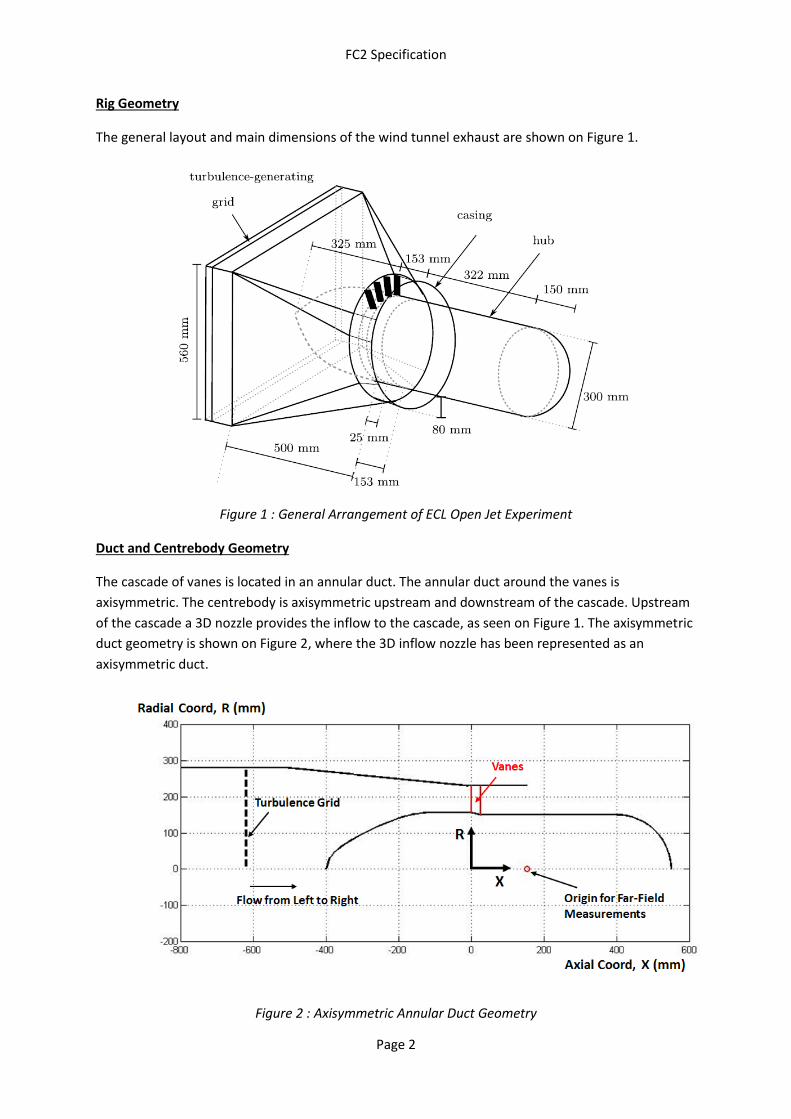
The general layout and main dimensions of the wind tunnel exhaust are shown on Figure 1.

Figure 1 : General Arrangement of ECL Open Jet Experiment

Duct and Centrebody Geometry

The cascade of vanes is located in an annular duct. The annular duct around the vanes is

axisymmetric. The centrebody is axisymmetric upstream and downstream of the cascade. Upstream

of the cascade a 3D nozzle provides the inflow to the cascade, as seen on Figure 1. The axisymmetric

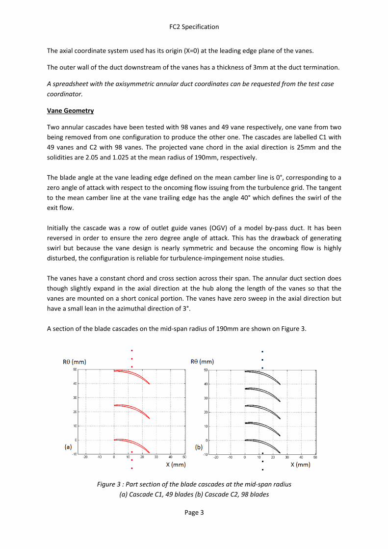
duct geometry is shown on Figure 2, where the 3D inflow nozzle has been represented as an

axisymmetric duct.

Figure 2 : Axisymmetric Annular Duct Geometry

FC2 Specification

The axial coordinate system used has its origin (X=0) at the leading edge plane of the vanes.

The outer wall of the duct downstream of the vanes has a thickness of 3mm at the duct termination.

A spreadsheet with the axisymmetric annular duct coordinates can be requested from the test case

coordinator.

Vane Geometry

Two annular cascades have been tested with 98 vanes and 49 vane respectively, one vane from two

being removed from one configuration to produce the other one. The cascades are labelled C1 with

49 vanes and C2 with 98 vanes. The projected vane chord in the axial direction is 25mm and the

solidities are 2.05 and 1.025 at the mean radius of 190mm, respectively.

The blade angle at the vane leading edge defined on the mean camber line is 0°, corresponding to a

zero angle of attack with respect to the oncoming flow issuing from the turbulence grid. The tangent

to the mean camber line at the vane trailing edge has the angle 40° which defines the swirl of the

exit flow.

Initially the cascade was a row of outlet guide vanes (OGV) of a model by-pass duct. It has been

reversed in order to ensure the zero degree angle of attack. This has the drawback of generating

swirl but because the vane design is nearly symmetric and because the oncoming flow is highly

disturbed, the configuration is reliable for turbulence-impingement noise studies.

The vanes have a constant chord and cross section across their span. The annular duct section does

though slightly expand in the axial direction at the hub along the length of the vanes so that the

vanes are mounted on a short conical portion. The vanes have zero sweep in the axial direction but

have a small lean in the azimuthal direction of 3°.

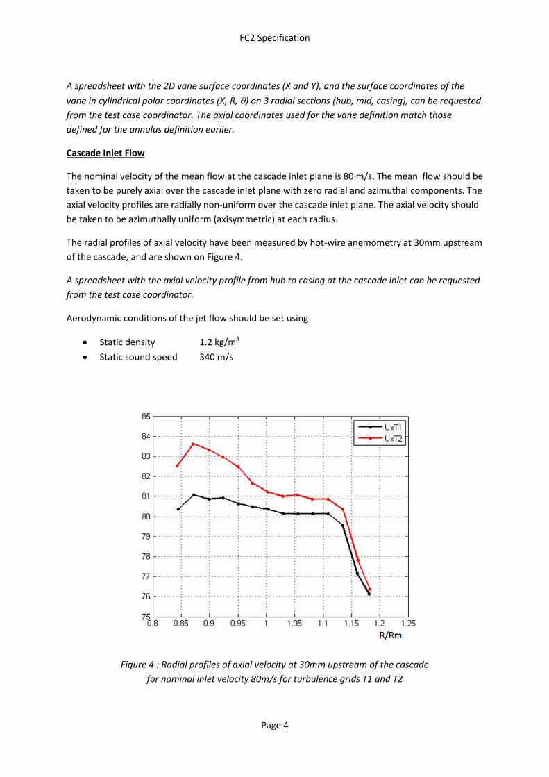
A section of the blade cascades on the mid-span radius of 190mm are shown on Figure 3.

Figure 3 : Part section of the blade cascades at the mid-span radius

(a) Cascade C1, 49 blades (b) Cascade C2, 98 blades

FC2 Specification

A spreadsheet with the 2D vane surface coordinates (X and Y), and the surface coordinates of the

vane in cylindrical polar coordinates (X, R, ) on 3 radial sections (hub, mid, casing), can be requested

from the test case coordinator. The axial coordinates used for the vane definition match those

defined for the annulus definition earlier.

Cascade Inlet Flow

The nominal velocity of the mean flow at the cascade inlet plane is 80 m/s. The mean flow should be

taken to be purely axial over the cascade inlet plane with zero radial and azimuthal components. The

axial velocity profiles are radially non-uniform over the cascade inlet plane. The axial velocity should

be taken to be azimuthally uniform (axisymmetric) at each radius.

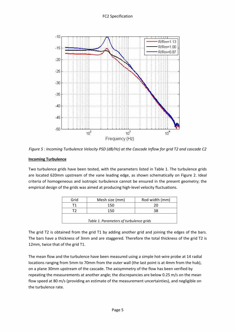
The radial profiles of axial velocity have been measured by hot-wire anemometry at 30mm upstream

of the cascade, and are shown on Figure 4.

A spreadsheet with the axial velocity profile from hub to casing at the cascade inlet can be requested

from the test case coordinator.

Aerodynamic conditions of the jet flow should be set using

Static density 1.2 kg/m3

Static sound speed 340 m/s

Figure 4 : Radial profiles of axial velocity at 30mm upstream of the cascade

for nominal inlet velocity 80m/s for turbulence grids T1 and T2

FC2 Specification

Figure 5 : Incoming Turbulence Velocity PSD (dB/Hz) at the Cascade Inflow for grid T2 and cascade C2

Incoming Turbulence

Two turbulence grids have been tested, with the parameters listed in Table 1. The turbulence grids

are located 620mm upstream of the vane leading edge, as shown schematically on Figure 2. Ideal

criteria of homogeneous and isotropic turbulence cannot be ensured in the present geometry; the

empirical design of the grids was aimed at producing high-level velocity fluctuations.

Grid Mesh size (mm) Rod width (mm)

T1 150 20

T2 150 38

Table 1. Parameters of turbulence grids

The grid T2 is obtained from the grid T1 by adding another grid and joining the edges of the bars.

The bars have a thickness of 3mm and are staggered. Therefore the total thickness of the grid T2 is

12mm, twice that of the grid T1.

The mean flow and the turbulence have been measured using a simple hot-wire probe at 14 radial

locations ranging from 5mm to 70mm from the outer wall (the last point is at 4mm from the hub),

on a plane 30mm upstream of the cascade. The axisymmetry of the flow has been verified by

repeating the measurements at another angle; the discrepancies are below 0.25 m/s on the mean

flow speed at 80 m/s (providing an estimate of the measurement uncertainties), and negligible on

the turbulence rate.

FC2 Specification

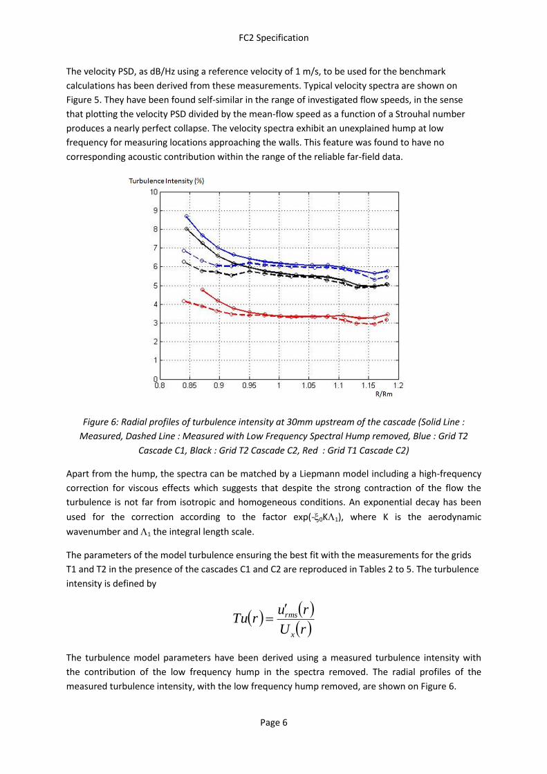
The velocity PSD, as dB/Hz using a reference velocity of 1 m/s, to be used for the benchmark

calculations has been derived from these measurements. Typical velocity spectra are shown on

Figure 5. They have been found self-similar in the range of investigated flow speeds, in the sense

that plotting the velocity PSD divided by the mean-flow speed as a function of a Strouhal number

produces a nearly perfect collapse. The velocity spectra exhibit an unexplained hump at low

frequency for measuring locations approaching the walls. This feature was found to have no

corresponding acoustic contribution within the range of the reliable far-field data.

Figure 6: Radial profiles of turbulence intensity at 30mm upstream of the cascade (Solid Line :

Measured, Dashed Line : Measured with Low Frequency Spectral Hump removed, Blue : Grid T2

Cascade C1, Black : Grid T2 Cascade C2, Red : Grid T1 Cascade C2)

Apart from the hump, the spectra can be matched by a Liepmann model including a high-frequency

correction for viscous effects which suggests that despite the strong contraction of the flow the

turbulence is not far from isotropic and homogeneous conditions. An exponential decay has been

used for the correction according to the factor exp(-0K1), where K is the aerodynamic

wavenumber and 1 the integral length scale.

The parameters of the model turbulence ensuring the best fit with the measurements for the grids

T1 and T2 in the presence of the cascades C1 and C2 are reproduced in Tables 2 to 5. The turbulence

intensity is defined by

rU

rurTu

x

rms

The turbulence model parameters have been derived using a measured turbulence intensity with

the contribution of the low frequency hump in the spectra removed. The radial profiles of the

measured turbulence intensity, with the low frequency hump removed, are shown on Figure 6.

FC2 Specification

Table 2 Characteristics of the turbulence of grid T1. in %, 1 in mm, 103x0. Cascade C1

r/Rm 0.84 0.87 0.895 0.92 0.95 0.975 1.00 1.02 1.06 1.08 1.11 1.13 1.16 1.18

4.63 4.07 3.87 3.78 3.68 3.61 3.63 3.60 3.53 3.49 3.36 3.18 3.14 3.22

1 23 21 20.5 19 17.5 17 17 16 16 16 15.5 15 16 17

0 14 14 14 14 14 14 14 14 14 13 13 10 0 0


r/Rm 0.84 0.87 0.895 0.92 0.95 0.975 1.00 1.02 1.06 1.08 1.11 1.13 1.16 1.18

6.87 6.33 6.06 6.03 6.20 6.09 6.05 6.00 5.96 5.97 5.86 5.71 5.31 5.46

1 23 23 22 20 20 19 19 19 19 19 19 17 19 19

0 20 20 20 20 18 18 18 18 17 16 15 13 13 10


r/Rm 0.84 0.87 0.895 0.92 0.95 0.975 1.00 1.02 1.06 1.08 1.11 1.13 1.16 1.18

4.16 3.90 3.65 3.47 3.40 3.40 3.34 3.31 3.33 3.32 3.13 2.98 2.95 3.16

1 26 26 25 24 23 23 22 21 21 21 20 19 19 19

0 10 5 0 0 0 0 0 0 0 0 0 0 0 2


r/Rm 0.84 0.87 0.895 0.92 0.95 0.975 1.00 1.02 1.06 1.08 1.11 1.13 1.16 1.18

6.27 5.78 5.71 5.54 5.75 5.64 5.54 5.47 5.44 5.28 5.09 4.89 4.92 5.08

1 27 27 26 26 26 26 25 25 25 25 25 25 25 25

0 10 7 7 7 7 7 7 7 6 5 5 0 0 0

The characteristics of the turbulence differ not only for grids T1 and T2 but also when they are

measured with either the cascade C1 or C2 installed. In view of the very small thickness of the vanes

some potential effect at the location of the hot-wire measurements is not expected. But because

the cascade C2 has twice the vane number of the cascade C1, additional pressure losses are more

probably responsible for this effect.

A spreadsheet with the turbulence characteristics at a number of radial positions from hub to casing

for turbulence grids T1 and T2, and cascades C1 and C2, should be requested from the test case

coordinator.

Measured turbulence velocity spectra are only available for turbulence grids T1 and T2 with cascade

C2, and for turbulence grid T2 with cascade C1. The turbulence velocity spectra for turbulence grid

T1 with cascade C2 should also be used for grid T1 with cascade C1. The upstream effect of the

different cascades with grid T1 is weaker than that for grid T2.

A spreadsheet with the turbulent velocity spectra at a number of radial positions from hub to casing

for turbulence grids T1 and T2 for cascade C2, and for turbulence grid T1 for cascade C2, should be

requested from the test case coordinator.

FC2 Specification

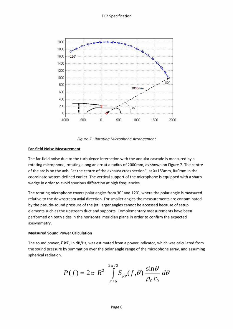
Figure 7 : Rotating Microphone Arrangement

Far-field Noise Measurement

The far-field noise due to the turbulence interaction with the annular cascade is measured by a

rotating microphone, rotating along an arc at a radius of 2000mm, as shown on Figure 7. The centre

of the arc is on the axis, “at the centre of the exhaust cross section”, at X=153mm, R=0mm in the

coordinate system defined earlier. The vertical support of the microphone is equipped with a sharp

wedge in order to avoid spurious diffraction at high frequencies.

The rotating microphone covers polar angles from 30° and 120°, where the polar angle is measured

relative to the downstream axial direction. For smaller angles the measurements are contaminated

by the pseudo-sound pressure of the jet; larger angles cannot be accessed because of setup

elements such as the upstream duct and supports. Complementary measurements have been

performed on both sides in the horizontal meridian plane in order to confirm the expected

axisymmetry.

Measured Sound Power Calculation

The sound power, PWL, in dB/Hz, was estimated from a power indicator, which was calculated from

the sound pressure by summation over the polar angle range of the microphone array, and assuming

spherical radiation.

dc

fSRfP pp

00

3/2

6/

2 sin),(2)(

FC2 Specification

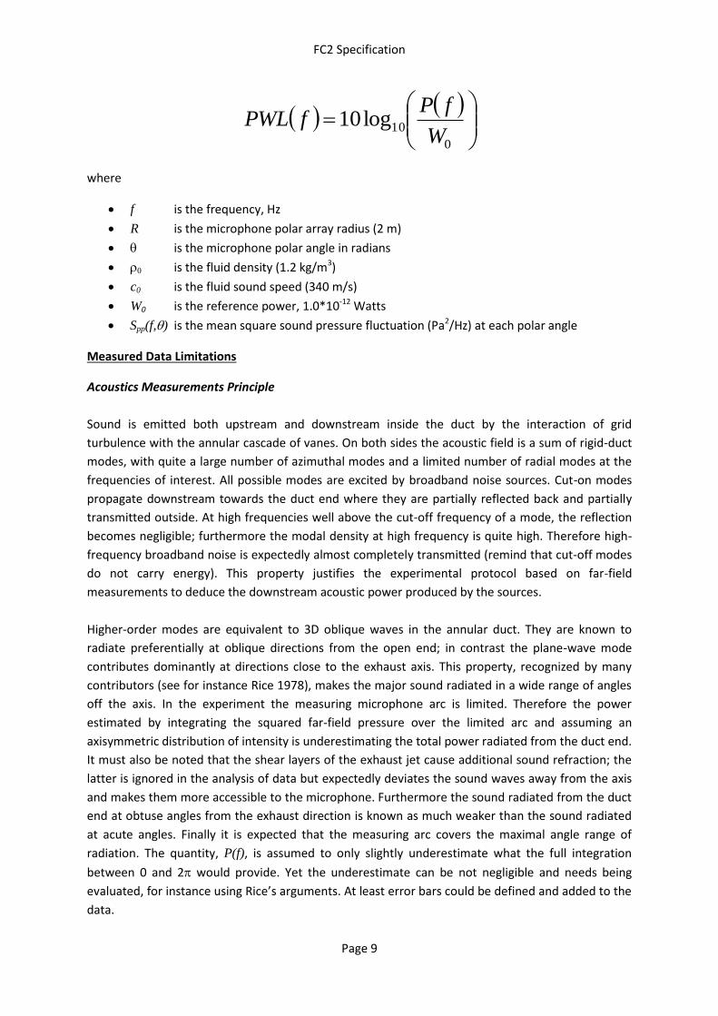
0

10log10W

fPfPWL

where

f is the frequency, Hz

R is the microphone polar array radius (2 m)

is the microphone polar angle in radians

is the fluid density (1.2 kg/m3)

c0 is the fluid sound speed (340 m/s)

W0 is the reference power, 1.0*10-12 Watts

Spp(f,) is the mean square sound pressure fluctuation (Pa2/Hz) at each polar angle

Measured Data Limitations

Acoustics Measurements Principle

Sound is emitted both upstream and downstream inside the duct by the interaction of grid

turbulence with the annular cascade of vanes. On both sides the acoustic field is a sum of rigid-duct

modes, with quite a large number of azimuthal modes and a limited number of radial modes at the

frequencies of interest. All possible modes are excited by broadband noise sources. Cut-on modes

propagate downstream towards the duct end where they are partially reflected back and partially

transmitted outside. At high frequencies well above the cut-off frequency of a mode, the reflection

becomes negligible; furthermore the modal density at high frequency is quite high. Therefore high-

frequency broadband noise is expectedly almost completely transmitted (remind that cut-off modes

do not carry energy). This property justifies the experimental protocol based on far-field

measurements to deduce the downstream acoustic power produced by the sources.

Higher-order modes are equivalent to 3D oblique waves in the annular duct. They are known to

radiate preferentially at oblique directions from the open end; in contrast the plane-wave mode

contributes dominantly at directions close to the exhaust axis. This property, recognized by many

contributors (see for instance Rice 1978), makes the major sound radiated in a wide range of angles

off the axis. In the experiment the measuring microphone arc is limited. Therefore the power

estimated by integrating the squared far-field pressure over the limited arc and assuming an

axisymmetric distribution of intensity is underestimating the total power radiated from the duct end.

It must also be noted that the shear layers of the exhaust jet cause additional sound refraction; the

latter is ignored in the analysis of data but expectedly deviates the sound waves away from the axis

and makes them more accessible to the microphone. Furthermore the sound radiated from the duct

end at obtuse angles from the exhaust direction is known as much weaker than the sound radiated

at acute angles. Finally it is expected that the measuring arc covers the maximal angle range of

radiation. The quantity, P(f), is assumed to only slightly underestimate what the full integration

between 0 and 2 would provide. Yet the underestimate can be not negligible and needs being

evaluated, for instance using Rice’s arguments. At least error bars could be defined and added to the

data.

FC2 Specification

Acquisitions

The measuring angles of the microphone are every 5° from 30° to 120° from the axis in the exhaust

direction. For smaller angles the measurements are contaminated by the pseudo-sound pressure of

the jet; larger angles cannot be accessed because of setup elements such as the upstream duct and

supports. Complementary measurements have been performed on both sides in the horizontal

meridian plane in order to confirm the expected axisymmetry.

The measured noise in the far-field includes both the broadband noise of interest emitted by the

annular cascade and radiated by the duct termination, and so-called background noise from

extraneous sources. The background noise is made of:

1) Residual noise produced by the flow through the turbulence grid, negligible in the present

case (isolated-airfoil noise studies at ECL with a turbulence grid installed upstream of an

open-jet anechoic facility led to similar conclusions).

2) Turbulent mixing noise from the jet

3) Low-frequency broadband noise due to flow separation and buffeting around the

hemispherical back-end, probably coupled with large-scale oscillations of the jet.

4) Trailing-edge noise generated as the turbulent flow developing inside the duct is convected

past the circular trailing edge of the nozzle. This contribution is present also in the

configuration of clean flow upstream of the cascade; in this case the turbulence is produced

in the vane wakes. The question of whether or not it significantly differs with and without

turbulence grid remains open.

Sources 2) and 3) are negligible at the low investigated Mach number and in the frequency range of

the turbulence impingement noise. Furthermore measurements made in clean inflow condition (no

turbulence grid) exhibit tones at very high frequencies that are attributed to laminar instabilities in

the cascade. The corresponding frequency range must be discarded from the analysis. In the data

post-processing, the broadband noise attributed to the turbulence-cascade interaction is obtained

by making the difference between the far-field spectra measured with and without turbulence grid.

This is based on the assumption that the background noise sources are not significantly modified

when introducing the grid, and that they are not correlated with turbulence-cascade interaction

noise. Due to all aforementioned issues, reliable values of the power indicator can only be obtained

in a limited frequency range.

Required Data to be Submitted to the Test Case Coordinator

The following data must be submitted to the test case coordinator for the specified test case input :

For turbulence grids T1 and T2, and then for cascades C1 and C2 for each turbulence grid

o Sound power PSD (PWL) spectrum in dB/Hz, calculated as described above, over the

frequency range 200-20000 Hz (use a reference power of 1.0*10-12 Watts for the

PWL dB calculation). The data should be provided to the test case coordinator as a

table of frequency versus PWL, either as a text file or in a spreadsheet. Data file

names should be of the form ‘FC2_”Contributor Name”_ TnCm_Far_Field_PWL_.......’,

FC2 Specification

where “n” and “m” correspond to the number of the turbulence grid and cascade

respectively.

Along with their results, contributors are requested to submit to the test case coordinator a 1 Slide

overview of their method used for this test case, including key assumptions and limitations, and

providing information on numerical methods and grids used where appropriate. The data file name

for the summary slides should be of the form ‘FC2_”Contributer_Name”_Overview_.......’

Optional Data to be Submitted to the Test Case Coordinator

If generated by the calculation method the following data may optionally be submitted to the test

case coordinator for the specified test case input :

For turbulence grids T1 and T2, and then for cascades C1 and C2 for each grid,

o Sound pressure PSD (SPL), in dB/Hz, at polar angles 30°, 60°, 90° and 120° over the frequency range 200-20000 Hz (use a reference pressure of 2.0*10-5 Pa for the SPL dB calculation). The data should be provided to the test case coordinator as a table of frequency versus SPL, either as a text files for each angle or in a spreadsheet. Data file names should be of the form ‘FC2_”Contributor Name”_ TnCm_Far_Field_SPL_.......’, where “n” and “m” correspond to the number of the turbulence grid and cascade respectively, or as ‘FC2_”Contributor Name”_ TnCm_Far_Field_SPL_Angle_aa_.......’ if in separate files, where “aa” is the polar angle in degrees.

o Sound pressure PSD (SPL), in dB/Hz, of the surface pressure around the vane over the frequency range 200-20000 Hz (use a reference pressure of 2.0*10-5 Pa for the SPL dB calculation) at the following chordwise locations on both the suction and pressure surfaces of the vane

1% chord 5% chord 20% chord 50% chord

The data should be provided to the test case coordinator as a table of frequency versus SPL, either as a text files for each chordwise position or in a spreadsheet. Data file names should be of the form ‘FC2_”Contributor Name”_ TnCm_Blade_SPL_.......’, where “n” and “m” correspond to the number of the turbulence grid and cascade respectively, or as ‘FC2_”Contributor Name”_ TnCm_Blade_SPL_pcChordX_pp_.......’ if in separate files, where the “X” is S or P for suction or pressure surface respectively, and “pp” is the percent chord value.

Measurements are not available for comparison with these calculated data, but comparison of the data between different calculation methods may shed light on the effectiveness of the methods.

Acknowledgements

The support of Prof. Michel Roger at ECL in setting up this test case for the broadband noise

benchmark programme is gratefully acknowledged.

FC2 Specification

References

1. Posson,H. & Roger,M., “Experimental Validation of a Cascade Response Function for Fan

Broadband Noise Predictions”, AIAA Journal, 49(9), 1907-1918, 2011

2. Rice,E.J., “Multimodal Far-Field Acoustic Radiation Pattern Using Mode Cut-off Ratio”, AIAA

Journal, 16(9), pp.906-911, 1978

Fan Stage Broadband Noise Benchmarking Programme ... · Fan Stage Broadband Noise Benchmarking...

Documents

Transcript of Fan Stage Broadband Noise Benchmarking Programme ... · Fan Stage Broadband Noise Benchmarking...