Extension of the Nonuniform Transformation Field Analysis ... · Extension of the Nonuniform...

Extension of the Nonuniform Transformation Field

Analysis to linear viscoelastic composites in the presence

of aging and swelling

Rodrigue Largenton, Jean-Claude Michel, Pierre Suquet

To cite this version:

Rodrigue Largenton, Jean-Claude Michel, Pierre Suquet. Extension of the Nonuniform Trans-formation Field Analysis to linear viscoelastic composites in the presence of aging and swelling.Mechanics of Materials, Elsevier, 2014, 73, pp.76-100. .

HAL Id: hal-00978984

https://hal.archives-ouvertes.fr/hal-00978984

Submitted on 15 Apr 2014

HAL is a multi-disciplinary open accessarchive for the deposit and dissemination of sci-entific research documents, whether they are pub-lished or not. The documents may come fromteaching and research institutions in France orabroad, or from public or private research centers.

L’archive ouverte pluridisciplinaire HAL, estdestinee au depot et a la diffusion de documentsscientifiques de niveau recherche, publies ou non,emanant des etablissements d’enseignement et derecherche francais ou etrangers, des laboratoirespublics ou prives.

https://hal.archives-ouvertes.fr

https://hal.archives-ouvertes.fr/hal-00978984

Extension of the Nonuniform Transformation Field Analysis to linear

viscoelastic composites in the presence of aging and swelling.

Rodrigue Largentona,∗, Jean-Claude Michelb, Pierre Suquetb

aMMC, EDF R&D Site des Renardieres, Avenue des Renardieres 77818 Moret sur Loing, France,

[email protected] de Mecanique et d’Acoustique, CNRS, UPR 7051, Aix-Marseille Univ, Centrale Marseille, 31,

Chemin Joseph Aiguier, 13402 Marseille Cedex 20, France, {michel,suquet}@lma.cnrs-mrs.fr

Abstract

This study presents a micromechanical modeling by the Nonuniform Transformation Field Anal-ysis (NTFA) of the viscoelastic properties of heterogeneous materials with aging and swellingconstituents. The NTFA proposed by Michel and Suquet (2003, 2004) is a compromise be-tween analytical models and full-field simulations. Analytical models, which are available onlyfor specific microstructures, provide effective constitutive relations which can be used in macro-scopic structural computations, but often fail to deliver sufficiently detailed information at smallscale. At the other extreme, full-field simulations provide detailed local fields, in addition tothe composite effective response, but come at a high cost when used in nested Finite ElementMethods. The NTFA method is a technique of model reduction which achieves a compromisebetween both approaches. It is based on the observation that the transformation strains (vis-cous strains, eigenstrains) often exhibit specific patterns called NTFA modes. It delivers botheffective constitutive relations and localization rules which allow for the reconstruction of localfields upon post-processing of macroscopic quantities.

A prototype of the materials of interest here is MOX (mixed oxides), a nuclear fuel which isa three-phase particulate composite material with two inclusion phases dispersed in a contigu-ous matrix. Under irradiation, its individual constituents, which can be considered as linearviscoelastic, are subject to creep, to aging (time dependent material properties) and to swelling(inhomogeneous eigenstrains). Its overall behavior is therefore the result of the combinationof complex and coupled phenomena. The NTFA is applied here in a three-dimensional settingand extended to account for inhomogeneous eigenstrains in the individual phases.

In the present context of linear viscoelasticity the modes can be identified following twoprocedures, either in each individual constituent, as initially proposed in Michel and Suquet(2003, 2004), or globally on the volume element, resulting into two slightly different models.

For non aging materials, the predictions of both models are in excellent agreement withfull-field simulations for various loading conditions, monotonic as well as non proportionalloading, creep and relaxation. The model with global modes turns out to be as predictive asthe original one with less internal variables. For aging materials, satisfactory results for the

∗Corresponding author. Tel: +33 442257382 ; fax: +33 442254747

Preprint submitted to Mechanics of Materials. March 10, 2014

overall as well as for the local response of the composites are obtained by both models at theexpense of enriching the set of modes. The prediction of the global model for the local fields isless accurate but remains acceptable. Use of the global NTFA model is therefore recommendedfor linear viscoelastic composites.

Keywords: Composite materials, viscoelasticity, aging, model reduction.

1. Introduction

Constitutive relations of solid materials are usually formulated at the engineering, or macro-scopic, scale. However, as the loadings become more complex, an accurate description of theirresponse requires the introduction of more internal variables, whose physical meaning is notalways clear and for which calibration of more material parameters is needed.

Micromechanical approaches provide an alternative to this phenomenological formulationof macroscopic constitutive relations, based on the observation that all solid materials are het-erogeneous at a small enough scale. The present study develops a micromechanically based,reduced model for the effective behavior of linear viscoelastic composites with individual con-stituents which, in addition to being viscoelastic, undergo aging and swelling. This is typicallythe case of the nuclear fuel MOX (mixed oxides) under irradiation. Our objective is to predictthe effective response of such composites under proportional and nonproportional mechanicalloadings as well as under irradiation where aging and swelling play an important role.

Micromechanical models for viscoelastic composites fall, roughly speaking, into one of threecategories:

1. Analytical models. For viscoelastic composites, the earlier analytical models can be tracedback to Hashin (1965) and Laws and Mc Laughlin (1978) where, using, the Laplace trans-form, the problem is reduced to finding the effective properties of elastic composites withmoduli depending on the Laplace parameter. It is now well-known that the effectiveproperties of linear viscoelastic composites with short memory gives rise to long memoryeffects (Sanchez-Hubert and Sanchez-Palencia, 1978; Suquet, 1987; Barbero and Luciano,1995). Even when the relaxation spectrum of the individual constituents is discrete (Diracmasses corresponding to a finite number of relaxation times), the effective spectrum ofthe composite may be a continuous functions with an infinite number of relaxation times(see Rougier et al., 1993; Beurthey and Zaoui, 2000; Masson et al., 2012, among others).Ricaud and Masson (2009) showed that for specific microstructures (two-phase compos-ites whose overall elastic properties are given by one of the Hashin-Shtrikman bounds) therelaxation spectrum of the composites remains discrete. This implies (Ricaud and Masson,2009; Vu et al., 2012) that the overall constitutive relations of such composites can bealternatively written with a finite number of internal variables. Conversely for compositeswith a continuous relaxation spectrum, an infinite number of internal variables is requiredand the advantage of an analytical model for subsequent use in a macroscopic numericalcomputation is lost. This has motivated the introduction of approximate models witha finite number of internal variables (or equivalently with a finite number of relaxation

2

times) mostly based on the approximation of the continuous relaxation spectrum by Pronyseries (Rekik and Brenner, 2011; Vu et al., 2012).

The main advantage of the analytical models, exact or approximate, when they requireonly a finite number of internal variables, is that their use in a numerical simulation is notsignificantly higher than that of usual linear viscoelastic constitutive relations (obviouslythis cost depends on the number of internal variables, or relaxation times, in the model).A first limitation of the analytical models for viscoelastic composites is that they makeuse of the Laplace transform to convert a viscoelastic problem into an elastic one. Thisprocedure does not apply rigorously to aging materials whose material properties dependon time. A second limitation of analytical models is that they only deliver the effectiveresponse of the composite and no information about the distribution of the fields (stress,strain) at the microscopic scale, except for the first moment (average) of the fields perphase. The same limitation applies to semi-analytical models based on the inclusionproblem (Kowalczyk-Gajewska and Petryk, 2011). However, a more detailed informationabout the statistics of the fields in the phases (field distribution, intra-phase standarddeviation) is often essential to predict the lifetime of structures which is governed bylocal values of the fields (damage or fracture). An approximation of the statistics of thefields in each phase up to second-order can be obtained by means of the effective internalvariable theory of Lahellec and Suquet (2007), Lahellec and Suquet (2013). However thislatter approach does not deliver effective constitutive relations and can only be used toobtain the response of the composite to a prescribed loading path.

2. Full-field simulations. The response (overall and local) of a representative volume ele-ment of the composite can be simulated directly (among many other references, see forinstance Michel et al., 1999; Zohdi and Wriggers, 2005; Gonzalez and Llorca, 2007, forcomputational micromechanics in general). For linear viscoelastic constituents the unit-cell problem is either solved as an elastic problem after use of the Laplace transform(Yi et al., 1998) or directly by a standard time-integration scheme. The advantage offull-field methods is that they account for all details of the microstructure and provide anaccurate (exact to round-off errors) description of the local fields. However, a first limi-tation of these methods is their computational cost. A second limitation is that full-fieldsimulations provide a constitutive update in a step-by-step time integration, but do notprovide a closed form expression for the constitutive relations. And even though the in-vestigation of three-dimensional complex microstructures has become a common practicein the recent years, the coupling between computations at the microscopic scale (mate-rial) and at the macroscopic scale (structure) is still the exception, despite the attemptsto perform computations at both scales simultaneously through nested Finite ElementMethods (FEM2, see Feyel, 1999; Feyel and Chaboche, 2000).

3. Reduced-order models. Reduced models aim at achieving a compromise between the twofirst class of approaches. On the one hand, they are based on numerical simulationsat the microscopic scale (which can sometimes be replaced by analytical calculations)and on the other hand they deliver constitutive relations with a finite number of inter-nal variables which can be used in macroscopic computations, at the expense of certain

3

approximations which depend on the reduction method. One of the earliest method ofthis type is the Transformation Field Analysis (TFA) of Dvorak (1992) further devel-oped in Dvorak et al. (1994) and extended to periodic composites by Fish et al. (1997).Assuming uniform eigenstrains within each individual constituent, Fish et al. (1997) de-rived an approximate scheme which they called, for a two-phase material, the two-pointhomogenization scheme. The original scheme and this extended scheme have been incor-porated successfully in structural computations (Dvorak et al., 1994; Fish and Yu, 2002;Kattan and Voyiadjis, 1993). However, it has been noticed that the TFA induces a spuri-ous kinematic hardening in the effective constitutive relations (Suquet, 1997) and that theapplication of the TFA to two-phase systems may require, in certain circumstances, a sub-division of each individual phase into several (and sometimes numerous) sub-domains toobtain a satisfactory description of the effective behavior of the composite (Michel et al.,2000; Chaboche et al., 2001; Michel and Suquet, 2003). The need for a finer subdivisionof the phases stems from the intrinsic nonuniformity of the plastic strain field whichcan be highly heterogeneous even within a single material phase. As a consequence, thenumber of internal variables needed to achieve a reasonable accuracy in the effective con-stitutive relations, although finite, is prohibitively high. In order to reproduce accuratelythe actual effective behavior of the composite, it is important to capture correctly theheterogeneity of the plastic strain field.

This last observation has motivated the introduction in Michel et al. (2000), Michel and Suquet(2003) of the Nonuniform Transformation Field Analysis (NTFA) where the (visco)plastic strainfield within each phase is decomposed on a finite set of plastic modes which can present largedeviations from uniformity. An approximate effective model for the composite can be derivedfrom this decomposition where the internal variables are the components of the (visco)plasticstrain field on the (visco)plastic modes. In addition, the NTFA provides localization rules whichallow for the reconstruction of local fields upon post-processing of macroscopic quantities and itcan predict local phenomena such as the distribution of the plastic dissipation at the microscopicscale (Michel and Suquet, 2009) under cyclic loading. A common feature shared by the TFA andthe NTFA is that these methods are applicable in situations where the superposition principleapplies, which in practice restrict their range of application to infinitesimal strains.

First applied to two-dimensional situations by Michel and Suquet (2004), the NTFA methodhas also been implemented in three-dimensional problems by Fritzen and Bohlke (2010) andextended to composites composed of a viscoelastic matrix containing elastic inclusions byFritzen and Bohlke (2013). By contrast with this latter work, the three phases consideredhere are all viscoelastic. This opens a new choice for the definition of the modes, which can bedefined in each individual constituents or over the whole volume element. Another distinctivefeature of the present work is that swelling and aging of the phases are explicitly taken intoaccount.

The paper is organized as follows. Section 2 presents the microstructure of MOX andthe behavior of its individual constituents. The NTFA procedure is recalled in section 3 andextended to account for swelling of the constituents. Two possible definitions of the modes,

4

either defined in each individual phase (as done in Michel and Suquet, 2003) and on the entirevolume element are introduced. The accuracy of both models is assessed by comparison withfull-field simulations in section 4 for non-aging materials and in section 5 for aging materials.

2. Three-phase particulate composites

Mixed oxide fuel, commonly referred to as MOX fuel, will serve to illustrate the theorydeveloped in this study. It is a nuclear fuel that contains more than one oxide of fissile material,usually consisting of plutonium blended with natural uranium, reprocessed uranium, or depleteduranium (Oudinet et al. , 2008). It is therefore of composite with, roughly speaking, threedistinct phases. A brief account on its microstructure and on the behavior of its individualconstituents is given here for the reader convenience.

2.1. Microstructure

(a) (b)

Figure 1: Maps of the Pu concentration in a 1 mm2 zone of a MOX pellet. (a) Longitudinal cross-section. b)Transverse cross-section.

MOX is a three-phase composite with a connected matrix containing two inclusion phasesdispersed in the matrix (Oudinet et al. , 2008). These phases are shown in Figure 1 obtainedby electon probe microanalysis (EPMA) where the different colors correspond to different con-centrations in plutonium. The three phases can be roughly described as follows:

1. The first inclusion phase (shown in red in Figure 1) is a plutonium rich phase with 25to 30 % of plutonium in mass. This phase will be referred to as the Pu clusters. Theswelling of these plutonium clusters under irradiation is quite significant. Their volumefraction in the composite is of the order of 15%. The diameter of Pu clusters varies inthe range [10µm, 70µm].

5

2. The second inclusion phase is a Plutonium poor phase and depleted Uranium rich (shownin blue in Figure 1). Its concentration in plutonium is less than 1 % in mass. It is calledthe U clusters. The swelling of this phase under irradiation is low. Its volume fractionin the composite is of the order of 25%. The diameter of the U clusters is of the order of30µm.

3. The matrix phase (shown in green in Figure 1) is intermediate between the two otherphases, with a moderate concentration in plutonium (typically 6 to 8 % in mass) andwith a moderate swelling strain under irradiation.

2.2. Individual constituents

In nominal conditions, the strains remain small and the total strain at a material point xin each of the phases can be decomposed into three contributions:

ε(x, t) = εe(x, t) + εv(x, t) + εs(x, t), (1)

where εe is the elastic strain, εv is the viscous strain due to creep of the material underirradiation and εs is the eigenstrain (or transformation strain) associated with solid swelling(due to irradiation here, but it could be a consequence of thermal or hygrometric effects in adifferent context). The elastic strain is related to the Cauchy stress σ by the elastic complianceM (inverse of the elastic stiffness L):

εe(x, t) = M (r) : σ(x, t) when x is in phase r. (2)

The creep strain is purely deviatoric and depends on the stress σ through a linear relationinvolving a shear viscosity G

(r)v which is a time dependent scalar, uniform in phase r,

εv(x, t) =1

2G(r)v (t)

s(x, t) in phase r, (3)

where s is the stress deviator. The time dependence of the shear viscosity G(r)v (t) is due to

aging and is discussed in Appendix C. The swelling strain is isotropic, uniform per phase anddepends on irradiation (and therefore is a function of time):

εs(x, t) = ε(r)s(t) i in phase r, (4)

where i is the second-order identity tensor. The three phases can be assumed to be isotropic andisotropically distributed in the matrix. To a good level of approximation their elastic moduli canbe assumed to be the same. However their viscosity and swelling coefficients differ significantly.For the same applied stress, the creep strains in the Pu clusters are approximately 2.5 timeslarger than in the matrix where they are 3 times larger than in the U clusters. Similarly theswelling strains in the Pu clusters are 3 times larger than in the matrix where they are 2.5larger than in the U clusters.

6

2.3. Reference results by full-field simulations

To the authors’ knowledge no complete experimental data are available for the mechanicalresponse of a volume element of irradiated MOX under complex loadings. Most available datapertain to actual pellets where the macroscopic fields (macroscopic strain, temperature) arenonuniform with an unknown spatial distribution. Therefore reference results for the effectiveresponse of these three-phase composites under mechanical and irradiation loadings have to begenerated using full-field simulations. For this purpose a volume element V of the compositeis chosen or generated in such a way that it respects all known statistical information on themicrostructure of the material. The response of this volume element to a mechanical andirradiation loading is simulated numerically on a time interval [0, T ] by solving the equilibriumand compatibility equations, together with the constitutive relations of the individual phasesand appropriate boundary conditions:

div(σ(x, t)) = 0, ε(x, t) = 12

(∇u+∇uT

),

σ(x, t) = L(x) : (ε(x, t)− εs(x, t)− εv(x, t)) ,

εs(x, t) =N∑

r=1

χ(r)(x) ε(r)s(t) i , εv(x, t) =

N∑

r=1

χ(r)(x)s(x, t)

2G(r)v (t)

u(x, t) = ε(t).x+ u∗(x, t) , u∗(x, t) # and σ(x, t).n(x) -# ,

(5)

where χ(r)(x) is the characteristic function of phase r. Periodic boundary conditions are as-sumed on the boundary of the volume element and this choice is reflected by the periodicity ofu∗ (notation #) and anti-periodicity of σ.n (notation -#) on the boundary of V .

The loading is specified by imposing the macroscopic strain path ε(t) and the irradiation

history (in other words the history ε(r)s (t) in each phase). The effective (or homogenized)

constitutive relations relate the overall stress σ(t) defined as the average of the local stress field

σ(t) = 〈σ(x, t)〉 = 1

|V |

∫

V

σ(x, t) dx,

to the history of the overall strain ε and of the swelling strains ε(r)s . As is well-known (and

discussed for instance in Michel et al., 1999), different loading conditions can be considered, forinstance by imposing the macroscopic stress history σ(t), or by imposing the direction of themacroscopic stress and the history of the macroscopic strain in the direction of the macroscopicstress. This latter type of loading, which corresponds for instance to a uniaxial tensile testwhere the strain the direction of the applied tension is controlled, is best suited for capturingsoftening effects in the macroscopic response (as it is the case for aging materials) and will beused in the examples of sections 4 and 5.

Generating one, or several, realizations of a “representative volume element” from micro-graphs of the actual microstructure of the material is an issue by itself. First a software has beendeveloped to process two-dimensional micrographs of the actual material such as those shownin figure 1 and to generate (periodic) artificial three-dimensional microstructures (figure 2).

7

The main ingredients of the tools developed for this purpose are presented in Largenton et al.(2010) and will not be discussed here in great details. The main steps of the procedure are asfollows:

1. First, the two-dimensional micrographs (such as that shown in figure 1) are analyzed: eachinclusion phase is segmented according to a procedure described in Oudinet et al. (2008).For each inclusion phase, the surface fraction is determined together with the distributionof diameters in each phase, assuming that each single inclusion can be approximated bya sphere (or a disk).

2. The three-dimensional distribution of diameters of each inclusion phase is deduced fromthe corresponding two-dimensional distribution by means of standard stereological rela-tions (see Saltykov, 1970, for instance).

3. A realization of the RVE is generated by the Random Sequential Adsorption Algorithmwith these data. All spherical inclusions are assumed to be impenetrable with a safetydistance 5 µm.

4. Finally the two-point correlation function for each realization is compared to the experi-mental one. The agreement is observed to be quite good (Largenton et al., 2010).

By contrast with the more elaborate procedure of Lee et al. (2009) where the two-point cor-relation function is used to define an error between the experimental data and the artificialrealization, here the two-point correlation function plays no role in the generation of the real-ization. However it serves to check a posteriori that both two-point correlation functions arein good agreement.

Eight realizations have been generated with the same statistical data namely 15% in volumefraction of Pu clusters with diameter in the range [10µm, 70µm], matching the experimentaldistribution of diameters, 25% in volume fraction of U clusters with 30µm in diameter, thevolume element being a cube with size (150µm)3. Each realization contains 121 Pu clusters ofdifferent sizes and 57 U clusters.

A parametric study of the effective response has been performed by a method based on fastFourier transforms which is a convenient alternative to Finite Elements for volume elementssubjected to periodic boundary conditions (Michel et al., 1999). It shows that the ratio betweenthe size of the volume element and that of the inclusions is sufficient to approach stationarityof the effective behavior with a good accuracy. Similarly it has been found that the statisticsof the field distribution in the different phases is also almost invariant from one realization toanother. Therefore a single realization (shown in figure 2) has been retained in the full-fieldsimulations.

A parametric study of the convergence of the results with respect to the discretization of thevolume element has been conducted in parallel. In the FFT method, a realization is an imagediscretized into equi-sized voxels and the discretization refers to the number of voxels presentin the image. Three different discretizations have been considered for a given realization,753, 1473 and 2453 voxels, and the response of the volume element to a tension-torsion test(test 1 in section 4) with swelling (but no-aging) has been simulated with the three different

8

discretizations. The results for the two finer discretizations showed no significant differencesand all subsequent simulations were performed with realizations discretized into 1473 voxels.

(a) (b)

Figure 2: Periodic realization of a three-dimensional volume element of MOX (discretized into 1473 pixels). (a)Inclusions only - Pu clusters (in red) U clusters (blue).( b) Entire volume element - matrix (green).

Typical material data for the individual phases used in the full-field simulations can befound in table 1. It should be noticed that the contrast in the swelling strain between the Pu

Phase E ν G(r)v ε

(r)s

(GPa) (-) (GPa.s) (s−1)Matrix (r=1) 200 0.3 52.94 7.00E − 05Pu clusters (r=2) 200 0.3 21.43 2.10E − 03U clusters (r=3) 200 0.3 158.83 2.84E − 05

Table 1: Material data for the individual phases.

clusters and the matrix used in the numerical simulations is artificially larger than in reality(30 instead of 3). This is done on purpose to magnify the effect of the mismatch between thephases.

3. NTFA models

3.1. Nonuniform transformation fields

The basic feature of the NTFA theory (Michel and Suquet, 2003, 2004) is a decompositionof the viscous strain on a set of a few, well-chosen, fields, called modes:

εv(x, t) =

M∑

k=1

ε(k)v(t) µ(k)(x) , (6)

9

where

• the modes(µ(k)(x)

)k=1,...,M

are incompressible tensorial fields (tr(µk))=0). The choice of

these modes is essential in the method and will be discussed in section 3.4.

• the(ε(k)v (t)

)k=1,...,M

’s are the generalized viscous strains associated with each mode for

which evolution equations will be derived (section 3.2).

Under the approximation (6), the determination of the field εv(x, t) reduces to the determi-

nation of the M tensorial variables ε(k)v (t). These variables are the internal variables of the

effective constitutive relations as will be clear from (17). In this sense, the NTFA is a methodfor model reduction. It should be emphasized that the number of modes M is chosen by theuser and is different from N , the number of phases in the composite.

Schematically, the NTFA proceeds in two successive steps:

• Choice of the modes. It will be seen in section 3.4 that two strategies are possible, eitherto define the modes on the entire volume element, or to choose the modes with supportin each individual constituent.

• Evolution equations for the generalized viscous strains. The evolution equation (3) forthe field of viscous strains has to be reduced to a set of differential equations for thegeneralized viscous strains. These differential equations are derived in section 3.2.

The outcomes are (see section 3.3):

• Explicit constitutive relations relating the overall stress σ(t) to the overall strain ε(t) and

to the generalized viscous strains(ε(k)v (t)

)

k=1,...,M. The macroscopic state variables of

the effective constitutive relations are therefore the observable variable ε and the internalvariables

(ε(k)v

)

k=1,...,M.

• Explicit expressions for the local stress and strain fields σ(x, t) and ε(x, t) in terms of

the state variables ε and(ε(k)v

)k=1,...,M

.

3.2. Reduced variables and evolution equations

Assume that the modes µ(k)(x) have been chosen (this choice is discussed in section 3.4).Then under the decomposition (6), it follows from the superposition principle that the localstrain field ε in the composite can be written as:

ε(x, t) = A(x) : ε(t) +M∑

ℓ=1

(D ∗ µ(ℓ))(x) ε(ℓ)v(t) +

N∑

r=1

(D ∗ χ(r)i)(x) ε(r)s(t) , (7)

where A(x) is the fourth-order tensorial field of elastic strain localization, ∗ denotes the con-volution product, D(x,x′) is the nonlocal operator expressing the strain at point x resulting

10

from an eigenstrain at point x′. The strain localization tensor A(x) and the influence tensors(D ∗ µ(k)

)k=1,...,M

,(D ∗ χ(r)i

)r=1,...,N

can be computed once for all by solving 6+M+N linear

elasticity problems on the RVE (see Appendix B). The corresponding stress field reads as:

σ(x, t) = L(x) : A(x) : ε(t) +

M∑

ℓ=1

L(x) :((D ∗ µ(ℓ))(x)− µ(ℓ)(x)

)ε(ℓ)v(t)

+N∑

r=1

L(x) :((D ∗ χ(r)i)(x)− χ(r)(x) i

)ε(r)s(t) .

(8)

The reduced stress associated with the k-th mode is defined as

τ (k)(t) = 〈µ(k)(x) : σ(x, t)〉.

Using eq. (8), the following relation is obtained:

τ (k)(t) = a(k) : ε(t) +

M∑

ℓ=1

(D(kℓ) − L(kℓ))ε(ℓ)v(t) +

N∑

r=1

(H(kr) − J (kr))ε(r)s(t) . (9)

where

a(k) = 〈µ(k) : L : A〉, D(kℓ) = 〈µ(k) : L : (D ∗ µ(ℓ))〉, L(kℓ) = 〈µ(k) : L : µ(ℓ)〉,H(kr) = 〈µ(k) : L : (D ∗ χ(r)i)〉, J (kr) = 〈µ(k) : L : χ(r) i〉.

}(10)

Using the constitutive equation (3) for the viscous strain-rate, the following relation betweenthe τ (k)’s and the ε(ℓ)’s is obtained:

τ (k)(t) = 〈µ(k)(x) : σ(x, t)〉 =M∑

ℓ=1

V (kℓ)(t)ε(ℓ)v(t), (11)

where the incompressibility of the modes has been used and V (kℓ) = 〈2Gv µ(k) : µ(ℓ)〉. Con-

versely

ε(ℓ)v(t) =

M∑

m=1

W (ℓm)(t)τ (m)(t) where W = V −1. (12)

Taking the time derivative of (9) and using (12), a differential equation for the τ (k)’s is obtained:

τ (k)(t)−M∑

ℓ=1

M∑

m=1

(D(kℓ) − L(kℓ))W (ℓm)(t)τm(t) = a(k) : ε(t) +N∑

r=1

(H(kr) − J (kr))ε(r)s(t) . (13)

Therefore the τ (k)’s solve a systems of differential equation of order one where the forcing termis the prescribed history of ε and ε

(r)s . A similar differential system for the ε

(k)v ’s can be obtained

by means of the relation (12). The history of the internal state variables (ε(k)v (t))|k=1,...,M is

completely determined by the resolution of these differential equations.

11

3.3. Effective response and local fields

The local stress and strain field can be expressed in terms of the state variables by meansof relations (8) and (7) which can be re-written in a more compact form as:

ε(x, t) = A(x) : ε(t) +

M∑

ℓ=1

η(ℓ)(x) ε(ℓ)v(t) +

N∑

r=1

ξ(r)(x) ε(r)s(t) , (14)

and

σ(x, t) = L(x) : A(x) : ε(t) +M∑

ℓ=1

ρ(ℓ)(x) ε(ℓ)v(t) +

N∑

r=1

ζ(r)(x) ε(r)s(t) (15)

where

η(ℓ)(x) = D ∗ µ(ℓ)(x), ξ(r)(x) = D ∗ χ(r)i(x),

ρ(ℓ)(x) = L(x) :(η(ℓ)(x)− µ(ℓ)(x)

), ζ(r)(x) = L(x) : (ξr(x)− χr(x)i) .

(16)

Finally the overall stress is obtained by averaging the local stress field (8):

σ(t) = L : ε(t) +M∑

k=1

〈ρ(k)〉 ε(k)v(t) +

N∑

r=1

〈ζ(r)〉 ε(r)s(t) , (17)

with (as is classical) L = 〈L : A〉.

3.4. Selection of the modes

The choice of the modes plays a key-role in the efficiency of the method. There is nouniversal choice for these modes and they should rather be chosen according to the type ofloading which the structure is likely to be subjected to. This implies that the user should havea rough a priori estimate of the domain of variation of the macroscopic strain (or stress), aswell as of the intensity of the swelling and of the aging of the phases (variation of the viscousmoduli along time). This domain of variation is explored numerically, not in its entirety, butalong specific paths, in the same way as an experimentalist would perform uniaxial or multiaxialtests to calibrate a constitutive model. For instance, in the case of swelling, the modes shouldincorporate information about the response of the volume element under pure swelling of thephases. Similarly if one is interested in the response of the structure under monotonic loadingwith limited amplitude, the information about the response of the unit-cell will be limited tocertain monotonic loading paths in stress space up to a limited amount of deformation. In theabsence of such information, standard test should be performed. Given the complexity of themicrostructures under consideration, the modes are not determined analytically but numericallyfrom actual viscous strain fields in the unit-cell.

12

3.4.1. Snapshot method

The modes are selected by the Karhunen-Loeve method applied to snaphsots of the viscousstrains along certain loading paths. This procedure of selection is sometimes referred to asthe Proper Orthogonal Decomposition (POD) snapshot method, widely used in the scientificcomputing community (pattern recognition, statistical analysis of data....). It seems to havebeen rediscovered several times under different names (Sirovich, 1987). It is perhaps bestknown in Fluid Mechanics (Sirovich, 1987; Berkooz et al., 1993; Holmes et al., 1996) and itsuse in Solid Mechanics is more recent. It was not known to the authors of the first versionof the NTFA method (Michel and Suquet, 2003). The POD has been extended in variousdirections, including the Proper Generalized Decomposition method where the shape functionschange with time and are computed on-the-fly (Chinesta et al., 2011; Ladeveze et al., 2010).The simplest version of the Karhunen-Loeve method is sufficient here for our purpose.

To keep the loading conditions rather general, monotonic loadings of the volume elementare simulated along given directions in the space of overall loadings, consisting of the overallstress σ and of the swelling of the individual phases. In the present study, 6 purely mechanicalloading paths have been defined by loading the volume element along 6 stress “directions” Σ0

s

with no swelling of the phases,

σ(t) = σ(t)Σ0s, ε(r)

s= 0 in each phase, (18)

with1 ≤ s ≤ 3 : Σ0

s = es ⊗ es,

and

4 ≤ s ≤ 6 : Σ0s =

1

2(ei ⊗ ej + ej ⊗ ei) , s = 9− i− j,

whereas the 7-th test correspond to pure swelling of the phases with no overall stress,

Σ07 = 0, ε(r)

sas in Table 1 for each phase.

The first 3 stress directions correspond to uniaxial tension in the three different directions andthe next 3 stress directions correspond to pure shear. Numerical simulations are carried outalong these paths by increasing monotonically the strain in the direction of the applied stress(except for the loading case 7) up to 10 % deformation along the applied stress for the 6 firstloading paths ε : Σ0 = 10%, and up to t = 10 s for the 7-th loading path. For the first 6 loadingpaths the overall strain-rate is fixed ε : Σ0 = 10−2s−1 so that 10 % deformation is attained in10 s. The material data used in these simulations can be found in Table 1.

For each loading case Σ0, snapshots θ(k)|k=1,..P of the viscous strain field are saved forfurther processing at different values of the strain ε : Σ0 along the applied stress Σ0. These

snapshots are normalized i.e. divided by 〈θ(k)eq 〉 where θeq =(23θijθij

)1/2(recall that the viscous

strains are incompressible). At the end of each simulation of a given loading case, P snapshotsare stored (and normalized). In the present study, the snapshots are stored every 0.4 s andtherefore P = 25 (each test lasts 10 s).

The actual modes are then extracted from these snapshots by means of the Karhunen-

Loeve (K-L) transform (or Proper Orthogonal Decomposition) which is well documented in theliterature (see for instance Holmes et al., 1996).

13

First the P × P correlation matrix between the snapshots for the same loading path isformed

g(kℓ) = 〈θ(k)(x) : θ(ℓ)(x)〉, k, ℓ = 1, . . . , P ,

and its eigenvalues λ(k) and eigenvectors v(k) are computed. The actual modes are expressedas a combination of the eigenvectors as

µ(k)(x) =P∑

ℓ=1

v(k)ℓ θ(ℓ)(x) . (19)

Note that the modes, as the eigenvectors of the symmetric matrix g, are orthogonal to eachother. Another well-known feature of the K-L transform is that the quantity of relevant infor-mation (its correlation with the set of snapshots) contained in an eigenvector v(k) is expressedby the magnitude of the corresponding eigenvalue λ(k). This property can be used to truncatethe set of modes, retaining the most relevant ones. Ordering the eigenvalues in decreasing order,the M modes corresponding to the largest eigenvalues can be selected by applying a thresholdcriterion

M∑

k=1

λ(k)/

(P∑

k=1

λ(k)

)≥ α,

In the present study α = 0.9999 = 1− 10−4.

A first application of the K-L transform is performed with the snapshots correspondingto the same loading path. The resulting modes are mutually orthogonal, but not necessarilyorthogonal to the modes corresponding to the other loading paths. Then the K-L transform isapplied a second time with the modes selected for each loading path as new snapshots. Onecould think that the same result would be achieved by applying the K-L transform in one stepto all snapshots mixing all loading paths, but this is not the case. Our experience is that themost accurate predictions are obtained with the modes generated by a double application ofthe K-L transform.

In conclusion, after (re-iterated) application of the Karhunen-Loeve transform, M modeshave been constructed. These modes are orthogonal to each other, they are incompressible andnormalized:

〈µ(k) : µ(ℓ)〉 = 0 k 6= ℓ, 〈µ(k)eq 〉 = 1, tr(µ(k)) = 0.

3.4.2. Local or global modes?

In the early version of the NTFA (Michel and Suquet, 2003), deviced for nonlinear con-stituents, the modes are defined independently in each individual phase. The restrictions of thesnapshots of the viscous strains to each individual phase are stored and processed by the K-Ltransform. In other words, there are as many sets of modes as phases. The independence of themodes from one phase to the other is essential in deriving the systems of differential equationsfor the reduced stress τ (k) whose evolution is governed by the other reduced stresses from the

same phase (projection of the stress on the modes in a given phase) but not by those of theother phases. In this sense, this earlier approach leads to local modes defined independently inthe different phases.

14

In the present study where the phases have a linear behavior, the differential equations forthe reduced stresses can be derived without the assumption that the modes are localized ina single phase (see the derivation of eq. (13) where the linearity of the relation between theviscous strain and the stress plays a crucial role). Therefore the modes can alternatively bedefined over the whole volume element V . These modes will be called global modes. Note thatthe above mentioned local modes are not simply the restriction to each phase of the globalmodes.

Both definitions of modes, local or global, have been used in the course of the present study.

1. For the local modes which is the original setting of the NTFA (Michel and Suquet, 2003),we have 7 loading paths, 25 snapshots per paths and 3 phases, hence a total of 525snapshots. After the first application of the K-L transform and with the threshold valueα = 0.9999, the K-L transform selects 3 modes for each loading path, hence a total of 21modes per phase, and 63 modes for the 3 phases altogether. When the K-L transform isrun for the second time, phase by phase, but combining the 21 modes obtained for thedifferent loading paths, 18 new modes are generated for each individual phase, hence atotal of 54 modes for the 3 phases.

2. The same procedure is followed for the global modes approach. To achieve the samerequired accuracy α, 3 modes are required for each loading path, hence a total of 21modes. Then, when the K-L transform is run again on these 21 modes, 18 modes aregenerated.

The two approaches are illustrated in Figure 3. The first modes extracted in each phase by theapplication of the K-L transform (iterated) are shown in subfigures (a), (b) and (c). The lastsubfigure (d) shows the first global mode over the whole volume element for the same loadingpath. As can be seen the local modes are not just the restriction to the phases of the globalmode.

The approach by global modes requires less internal variables at the macroscopic scale (18internal variables instead of 54) and it is certainly more attractive from the point of view ofthe cost of the structural calculations performed with the effective constitutive relations (17).However, before concluding in favor of the global approach, it is worth comparing the accuracyof both approaches on more complex loading paths, with or without aging of the constituents.

4. Non-aging constituents

To check the accuracy of the two NTFA approaches, with global and local modes respec-tively, four tests have been performed. In this section, aging of the constituents is not takeninto account.

Test 1. Radial monotonic loading along a stress direction which has not been used for the iden-tification of the modes, involving tension and torsion along the first axis:

Σ0 =1√2(e1 ⊗ e1 + e1 ⊗s e2 + e1 ⊗s e3) . (20)

The volume element is loaded at constant strain-rate ε : Σ0 = (1/√2)10−2s−1 for 10 s.

15

(a) (b)

(c) (d)

Figure 3: Snapshot of µ(1)eq . (a): First local mode in phase 1 (matrix). (b): First local mode in phase 2 (Pu

clusters). (c): First local mode in phase 3 (U clusters). (d): First global mode.

16

Test 2. A creep test in uniaxial tension in direction 3:

Σ0 = e3 ⊗ e3.

First a linear ramp is applied in 0.1 s from σ33 = 0 to σ33 = 100 MPa. Then σ33 is keptfixed (= 100 MPa).

Test 3. A relaxation test under uniaxial tension (σij = 0, except σ33). The overall strain indirection 3 is increased in 0.1 s from 0 to ε33 = 0.02 and kept constant.

Test 4. A non radial test involving a rotation of principal axes of the overall stress. The overallstrain is imposed in the form

ε(t) = ε0 sinωt

[e1 ⊗ e1 −

1

2e2 ⊗ e2 −

1

2e3 ⊗ e3

]+ε0(1−cos(ωt)) [e1 ⊗s e2 + e1 ⊗s e3] ,

(21)with ε0 = 0.1, ω = π

2. Swelling is not activated. The response of the volume element is

investigated for the first 5 cycles (20 s).

For all 4 tests, the predictions of the two NTFA approaches (with global or local modes) arecompared with reference results obtained by full-field simulations using the material data inTable 1. For completeness, the predictions of the TFA method (where the viscous strain isassumed to be uniform within each individual phase) have also been added for Test 1.

The comparison is carried out for three types of information:

i) the effective response of the composite,

ii) the average response of the phases,

iii) the distribution of the stress field in the phases.

4.1. Effective response

The predictions of the two NTFA approaches, with global and local modes, for the overallresponse of the composite are compared in Figure 4. In Figure 4(a), the prediction of the TFAis also shown. The following comments can be made:

1. The predictions of the TFA deviate significantly from the full-field simulations.

2. Both NTFA approaches are in excellent agreement with the reference results. In otherwords, the coarser model (NTFA with global modes with 18 internal variables) is asaccurate as the finer one (NTFA with modes per phase with 54 internal variables), atleast for predicting the effective response of the composite.

3. It worth noting that although the modes have been generated from a set of snapshotscorresponding to monotonic loading along specific directions, the NTFA models are stillaccurate for the more complex loadings of tests 2, 3, 4.

4. The same conclusion applies with or without swelling in the phases.

17

0.0

0.1

0.2

0.3

0.4

0.5

0.6

0.7

0.8

0.9

1.0

1.1

1.2

||σ||(G

Pa)

0 1 2 3 4 5 6 7 8 9 10

t (s)

Tension-torsion + swelling

Full-field

NTFA local modes

NTFA global modes

TFA

(a)

0.0

0.001

0.002

0.003

0.004

0.005

0.006

0.007

0.008

0.009

0.01

ε 33

0 1 2 3 4 5 6 7 8 9 10

t (s)

Creep test

NTFA local modes

NTFA global modes

Full-field

with swelling

without swelling

(b)

-0.5

0.0

0.5

1.0

1.5

2.0

2.5

3.0

3.5

4.0

σ33

(GPa)

0 1 2 3 4 5 6 7 8 9 10

t (s)

Relaxation testNTFA local modes

NTFA global modes

Full-field

without swelling

with swelling

(c)

-10.0

-7.5

-5.0

-2.5

0.0

2.5

5.0

7.5

10.0

σ13

(GPa)

-15 -10 -5 0 5 10 15

σ11 (GPa)

Rotation of the principal axes of stress

(no swelling)

Full-field

NTFA local modes

NTFA global modes

(d)

Figure 4: Non-aging constituents - Effective response. Comparison between full-field simulations (symbols) andthe two NTFA approaches with global modes (dashed line) and with local modes (dotted line). (a): Test 1. (b)Test 2. (c): Test 3. (d): Test 4.

18

4.2. Average response of the phases

The average of the stress in the three different phases are compared in Figure 5a, c, d fortests 1, 3, 4 and the average strain in the phases is shown in Figure 5b. The norm of the averagestress σ(r) in each constituent is used for this comparison:

σ(r)ij =

1

Vr

∫

Vr

σij(x) dx,∣∣∣∣σ(r)

∣∣∣∣ =(

3∑

i,j=1

σ(r)ij σ

(r)ij

)1/2

. (22)

The predictions of the TFA are clearly unrealistic and will not be investigated further. Theagreement of the two NTFA approaches with the reference results is again excellent, both withswelling and without swelling. In test 3 (relaxation), both approaches are able to capture thequick relaxation of stress in the the Pu phase, followed by a progressive reloading of this phase,consequence of swelling and of the relaxation of the two other phases. This illustrates the factthat even though the overall loading is monotonic, the local response in the phases can be quitecomplex, a complexity that the NTFA captures well.

4.3. Local stress fields

The local stress fields in the phases at the end of test 1 (at t=10 s) and test 4 (at t=20 s)reconstructed by means of the relation (15) are compared in Figures 6, 7 and 8 where the localnorm of σ, defined as

||σ(x)|| =(

3∑

i,j=1

σij(x)σij(x)

)1/2

, (23)

is plotted. They can hardly been distinguished. It is only when comparing the probabilitydistribution of the stress fields in the phases that a slight discrepancy can be observed. Thisis done in Figure 9 for test 1 and Figure 10 for test 4. The NTFA approach with local modes(dotted line) fits well the full-field simulations, whereas a little deviation can be seen withthe NTFA approach with global modes. But the discrepancy remains small (compared to thedispersion of the results for different realizations, see Appendix A) and both NTFA approachescan be considered as being in excellent agreement with the reference results.

4.4. Gain in computational time

The CPU times for the different methods (TFA, NTFA with global modes, NTFA with localmodes and full-field simulations) have been compared for Test 1. The different CPU times (IntelCore i7-2920XM) are as follows:

• Full-field simulations (discretization in 1473 voxels): 1231 s.

• TFA (18 internal variables): 0.018s.

• NTFA with local modes (54 internal variables): 0.64s.

• NTFA with global modes (18 internal variables): 0.046 s.

19

0.0

0.2

0.4

0.6

0.8

1.0

1.2

1.4

1.6

1.8

∣ ∣ ∣ ∣∣ ∣ ∣ ∣σ(r)∣ ∣ ∣ ∣∣ ∣ ∣ ∣(G

Pa)

0 1 2 3 4 5 6 7 8 9 10

t (s)


Full-field

NTFA local modes

NTFA global modes

TFA

Matrix (phase 1)

U clusters (phase 3)

Pu clusters (phase 2)

(a)

0.0

0.005

0.01

0.015

0.02

0.025

0.03

0.035

0.04

∣ ∣ ∣ ∣∣ ∣ ∣ ∣ε(r)∣ ∣ ∣ ∣∣ ∣ ∣ ∣

0 1 2 3 4 5 6 7 8 9 10

t (s)

Creep + swellingNTFA local modes

NTFA global modes

Full-field

Matrix (phase 1)



(b)

0.0

0.5

1.0

1.5

2.0

2.5

3.0

3.5

4.0

∣ ∣ ∣ ∣∣ ∣ ∣ ∣σ(r)∣ ∣ ∣ ∣∣ ∣ ∣ ∣(G

Pa)

0 1 2 3 4 5 6 7 8 9 10

t (s)

Relaxation + swellingNTFA local modes

NTFA global modes

Full-field

Matrix (phase 1)



(c)

-10.0

-7.5

-5.0

-2.5

0.0

2.5

5.0

7.5

10.0

σ(r)

13(G

Pa)

-15 -10 -5 0 5 10 15

σ(r)11 (GPa)

Rotation of the principal axes of stress

(no swelling)

Last cycle

Full-fieldNTFA local modesNTFA global modes

Matrix

Pu clusters

U clusters

(d)

Figure 5: Non-aging constituents -Average response of the phases. Comparison between full-field simulations(symbols), the NTFA approach with global modes (dashed line) and the NTFA approach with local modes(dotted line). (a): Test 1. (b): Test 2. (c): Test 3. (d): Test 4, last cycle.

20

(a) (b) (c)

Figure 6: Non-aging constituents. Norm of the stress field in the matrix (units: GPa). (a): Full-field. (b):NTFA with local modes. (c): NTFA with global modes.

(a) (b) (c)

Figure 7: Non-aging constituents. Norm of the stress field in the Pu clusters (units: GPa). (a): Full-field. (b):NTFA with local modes. (c): NTFA with global modes.

(a) (b) (c)

Figure 8: Non-aging constituents. Norm of the stress field in the U clusters (units: GPa). (a): Full-field. (b):NTFA with local modes. (c): NTFA with global modes.

21

0.0

0.01

0.02

0.03

0.04

0.05

0.06

0.07

0.08

0.09

0.1

0.11

0.12

Frequency

0.25 0.5 0.75 1.0 1.25 1.5 1.75 2.0 2.25 2.5 2.75 3.0

||σ|| (GPa)

Tension-torsion without aging, with swelling

t = 10 s

Full-field

NTFA local modes

NTFA global modes

Matrix (phase 1)



Figure 9: Non-aging constituents. Test 1. Probability distribution of the norm of the stress field in the differentphases at t = 10 s.

0.0

0.01

0.02

0.03

0.04

0.05

0.06

0.07

0.08

0.09

0.1

0.11

Frequency

7.5 8.75 10.0 11.25 12.5 13.75 15.0 16.25 17.5

||σ|| (GPa)

Rotation of the principal axes of stress,

without aging, without swelling

t = 20 s

Full-field

NTFA local modes

NTFA global modes

Matrix (phase 1)



Figure 10: Non-aging constituents - Test 4 - Probability distribution of the norm of the stress field in thedifferent phases at t = 20s.

22

The TFA is the costless method but is, by far, too inaccurate. Its accuracy can be improvedby subdividing the phases into several subdomains but then its costs will be much larger thanthat of the NTFA with less accuracy. The gain in CPU times obtained by using the NTFA withglobal modes over the full-field simulations is 2× 104. This is quite significant. Finally the twoNTFA methods with local and global modes differ in cost by a factor of 10 approximatively.

4.5. Conclusions

For non-aging constituents the predictions of both NTFA approaches, with modes defined inthe whole volume or per phase, with or without swelling in the phases, are in excellent agreementwith full-field simulations over a wide variety of loading paths. Given that the NTFA with globalmodes has less internal variables (18 instead of 54 in the NTFA approach wih local modes), theuse of this reduced model seems amply sufficient for macroscopic structural calculations. Theobjective of the next section is to check the validity of this conclusion for aging constituents.

5. Composites with aging constituents

When the constituents of the composite are subject to aging, care should be used in thechoice of the modes on which the decomposition (6) is based. By construction the modes donot depend on time, unlike the material properties of the constituents which, because of aging,vary with time. Therefore it is not clear which material data should be used in the tests fromwhich the modes are constructed. A first possibility is to construct the modes as in section 4with the initial material properties of the phases and to keep them unchanged through the whole

evolution process of the material. The question which arises naturally is whether these modes,which are relevant in the initial stage of the deformation, contain sufficient information on thedeformation of the microstructure throughout the whole loading history. Another possibilitywould be to use the material data at the end of the aging history or the actual aging properties,whenever they are known, to generate the modes. A last possibility is to mix the two sets ofmodes obtained with the initial and final material properties. The aim of this section is toinvestigate these different possibilities.

5.1. Aging constituents

The level of aging of the constituents depends on the history of irradiation to which thefuel is subjected. Since irradiation is a known function of time, specifying an aging historyis equivalent to specifying a time dependence of the material properties of the constituents.Aging affects mostly the viscosity G

(r)v of the individual constituents (Scdap Relap5, 1997), or

equivalently their fluidity defined as 1/G(r)v , whereas the other material properties (elasticity,

swelling rate) can be considered as time independent.

Since aging softens the matrix (phase 1), the matrix fluidity increases with irradiation,corresponding to an acceleration of the creeping-rate. The increase in matrix fluidity withirradiation is a consequence of the increase in content of the plutonium (239 and 241) byneutron capture from uranium (238). To make things simple the variations of the matrixfluidity with respect to time on an interval of study [0, T ] are assumed to be bilinear, witha first linear ramp from 0 to a transition time t1 and a second ramp from t1 to the final

23

time T (see Appendix C). The two intervals [0, t1] and [t1, T ] correspond for instance to twodifferent regimes of irradiation. The first interval corresponds to the case where uranium (238)and plutonium (239 and 241) contents are hardly consumed. This regime of irradiation isrepresentative of low power pressure water reactor (PWR) conditions. The second intervalcorresponds to the case where the plutonium (239 and 241) and uranium (238) contents areconsumed. This regime of irradiation is representative of PWR nominal conditions. The specificexpression of G

(1)v (t) corresponding to the plots of Figure 11 is given in Appendix C. It was

obtained by the neutron model of the nuclear fuel code Cyrano3 (Baron et al., 2008).

2

5

10

2

5

102

2

5

G(r)

v(G

Pa.s)

0 1 2 3 4 5 6 7 8 9 10

t (s)

Scenario 1 Matrix (phase 1)



ζ=5

ζ=3

ζ=2

ζ=1

10

2

5

102

2

5

G(r)

v(G

Pa.s)

0 1 2 3 4 5 6 7 8 9 10

t (s)

Scenario 2 Matrix (phase 1)



ζ=0.5

ζ=0.1865

Figure 11: Aging constituents - Different scenarii for the evolution of G(r)v (t) with time for the three phases.

The U clusters follow the same trend as the matrix but creep 3 times slower since theplutonium content is lower. Therefore the viscosities of phase 1 and phase 3 are linked through

G(3)v(t) = 3G(1)

v(t),

and the evolution in time of the viscosity in the matrix and in the U clusters are parallel (Figure11).

As for the Pu phase, its viscosity is initially the lowest of the three phases (Table 1), whichcorresponds to creep eigenstrains in the Pu phase being 2.5 time larger than in the matrix.Two scenarii for the time-dependence of the creeping properties of the Pu phase have beeninvestigated corresponding either to softening or hardening of this phase relative to the matrix.These scenarii differ by the value of the parameter ζ which measures the variation of the

24

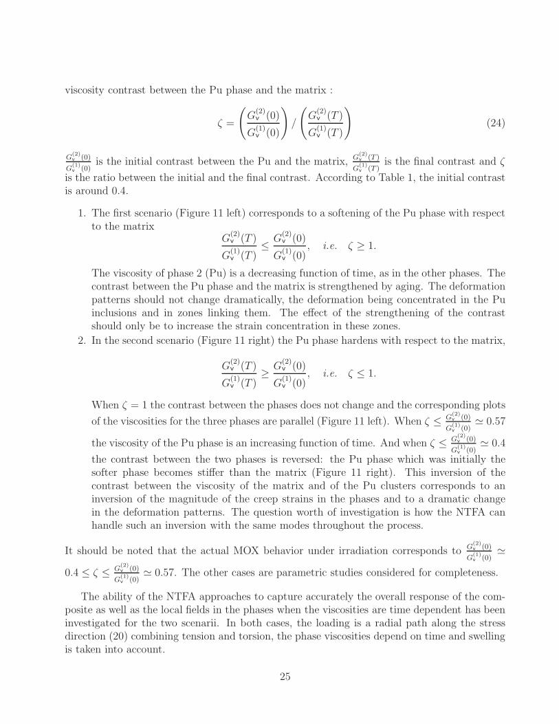
viscosity contrast between the Pu phase and the matrix :

ζ =

(G

(2)v (0)

G(1)v (0)

)/

(G

(2)v (T )

G(1)v (T )

)(24)

G(2)v (0)

G(1)v (0)

is the initial contrast between the Pu and the matrix, G(2)v (T )

G(1)v (T )

is the final contrast and ζ

is the ratio between the initial and the final contrast. According to Table 1, the initial contrastis around 0.4.

1. The first scenario (Figure 11 left) corresponds to a softening of the Pu phase with respectto the matrix

G(2)v (T )

G(1)v (T )

≤ G(2)v (0)

G(1)v (0)

, i.e. ζ ≥ 1.

The viscosity of phase 2 (Pu) is a decreasing function of time, as in the other phases. Thecontrast between the Pu phase and the matrix is strengthened by aging. The deformationpatterns should not change dramatically, the deformation being concentrated in the Puinclusions and in zones linking them. The effect of the strengthening of the contrastshould only be to increase the strain concentration in these zones.

2. In the second scenario (Figure 11 right) the Pu phase hardens with respect to the matrix,

G(2)v (T )

G(1)v (T )

≥ G(2)v (0)

G(1)v (0)

, i.e. ζ ≤ 1.

When ζ = 1 the contrast between the phases does not change and the corresponding plots

of the viscosities for the three phases are parallel (Figure 11 left). When ζ ≤ G(2)v (0)

G(1)v (0)

≃ 0.57

the viscosity of the Pu phase is an increasing function of time. And when ζ ≤ G(2)v (0)

G(1)v (0)

≃ 0.4

the contrast between the two phases is reversed: the Pu phase which was initially thesofter phase becomes stiffer than the matrix (Figure 11 right). This inversion of thecontrast between the viscosity of the matrix and of the Pu clusters corresponds to aninversion of the magnitude of the creep strains in the phases and to a dramatic changein the deformation patterns. The question worth of investigation is how the NTFA canhandle such an inversion with the same modes throughout the process.

It should be noted that the actual MOX behavior under irradiation corresponds to G(2)v (0)

G(1)v (0)

≃

0.4 ≤ ζ ≤ G(2)v (0)

G(1)v (0)

≃ 0.57. The other cases are parametric studies considered for completeness.

The ability of the NTFA approaches to capture accurately the overall response of the com-posite as well as the local fields in the phases when the viscosities are time dependent has beeninvestigated for the two scenarii. In both cases, the loading is a radial path along the stressdirection (20) combining tension and torsion, the phase viscosities depend on time and swellingis taken into account.

25

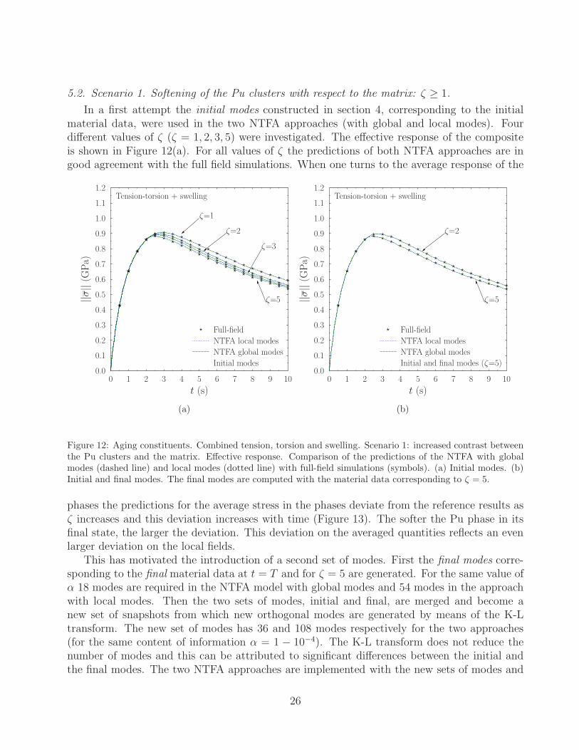
5.2. Scenario 1. Softening of the Pu clusters with respect to the matrix: ζ ≥ 1.

In a first attempt the initial modes constructed in section 4, corresponding to the initialmaterial data, were used in the two NTFA approaches (with global and local modes). Fourdifferent values of ζ (ζ = 1, 2, 3, 5) were investigated. The effective response of the compositeis shown in Figure 12(a). For all values of ζ the predictions of both NTFA approaches are ingood agreement with the full field simulations. When one turns to the average response of the

0.0

0.1

0.2

0.3

0.4

0.5

0.6

0.7

0.8

0.9

1.0

1.1

1.2

||σ||(G

Pa)

0 1 2 3 4 5 6 7 8 9 10

t (s)


Full-field

NTFA local modes

NTFA global modes

Initial modes

ζ=1

ζ=2

ζ=3

ζ=5

(a)

0.0

0.1

0.2

0.3

0.4

0.5

0.6

0.7

0.8

0.9

1.0

1.1

1.2

||σ||(G

Pa)

0 1 2 3 4 5 6 7 8 9 10

t (s)


Full-field

NTFA local modes

NTFA global modes

Initial and final modes (ζ=5)

ζ=2

ζ=5

(b)

Figure 12: Aging constituents. Combined tension, torsion and swelling. Scenario 1: increased contrast betweenthe Pu clusters and the matrix. Effective response. Comparison of the predictions of the NTFA with globalmodes (dashed line) and local modes (dotted line) with full-field simulations (symbols). (a) Initial modes. (b)Initial and final modes. The final modes are computed with the material data corresponding to ζ = 5.

phases the predictions for the average stress in the phases deviate from the reference results asζ increases and this deviation increases with time (Figure 13). The softer the Pu phase in itsfinal state, the larger the deviation. This deviation on the averaged quantities reflects an evenlarger deviation on the local fields.

This has motivated the introduction of a second set of modes. First the final modes corre-sponding to the final material data at t = T and for ζ = 5 are generated. For the same value ofα 18 modes are required in the NTFA model with global modes and 54 modes in the approachwith local modes. Then the two sets of modes, initial and final, are merged and become anew set of snapshots from which new orthogonal modes are generated by means of the K-Ltransform. The new set of modes has 36 and 108 modes respectively for the two approaches(for the same content of information α = 1 − 10−4). The K-L transform does not reduce thenumber of modes and this can be attributed to significant differences between the initial andthe final modes. The two NTFA approaches are implemented with the new sets of modes and

26

0.0

0.2

0.4

0.6

0.8

1.0

1.2

1.4

1.6

∣ ∣ ∣ ∣∣ ∣ ∣ ∣σ(r)∣ ∣ ∣ ∣∣ ∣ ∣ ∣(G

Pa)

0 1 2 3 4 5 6 7 8 9 10

t (s)


Full-field

NTFA local modes

NTFA global modes

Initial modes

ζ=2

Matrix (phase 1)



(a)

0.0

0.2

0.4

0.6

0.8

1.0

1.2

1.4

1.6

∣ ∣ ∣ ∣∣ ∣ ∣ ∣σ(r)∣ ∣ ∣ ∣∣ ∣ ∣ ∣(G

Pa)

0 1 2 3 4 5 6 7 8 9 10

t (s)


Full-field

NTFA local modes

NTFA global modes

Initial modes

ζ=5

Matrix (phase 1)



(b)

Figure 13: Aging constituents. Combined tension, torsion and swelling. Scenario 1: increased contrast betweenthe Pu clusters and the matrix. Average stress in the individual phases. Comparison between full-field simula-tions (symbols) and the two NTFA approaches, with global modes (dashed line) and with local modes (dottedline). Modes generated with the initial material data. (a): ζ = 2. (b): ζ = 5.

27

the predictions for ζ = 2 and ζ = 5 are shown in Figure 14. Even though the final modes havebeen computed only for ζ = 5, the agreement is excellent for ζ = 2 and ζ = 5, both for theeffective response (Figure 12(b)) and for the average stress in the phases (Figure 14). If we now

0.0

0.2

0.4

0.6

0.8

1.0

1.2

1.4

1.6

∣ ∣ ∣ ∣∣ ∣ ∣ ∣σ(r)∣ ∣ ∣ ∣∣ ∣ ∣ ∣(G

Pa)

0 1 2 3 4 5 6 7 8 9 10

t (s)


Full-field

NTFA local modes

NTFA global modes


ζ=2

Matrix (phase 1)



(a)

0.0

0.2

0.4

0.6

0.8

1.0

1.2

1.4

1.6

∣ ∣ ∣ ∣∣ ∣ ∣ ∣σ(r)∣ ∣ ∣ ∣∣ ∣ ∣ ∣(G

Pa)

0 1 2 3 4 5 6 7 8 9 10

t (s)


Full-field

NTFA local modes

NTFA global modes


ζ=5

Matrix (phase 1)



(b)

Figure 14: Aging constituents. Combined tension, torsion and swelling. Scenario 1: increased contrast betweenthe Pu clusters and the matrix. Average stress in the individual phases. Combination of initial and final modes(generated with the initial material data and with the final material data with ζ = 5)). Comparison betweenfull-field simulations (symbols) and the two NTFA approaches, with global modes (dashed line) and with localmodes (dotted line). (a): ζ = 2. (b): ζ = 5.

turn to more local informations, i.e. to the distribution of the stress field in the phases shownin Figure 15, it is observed that the NTFA model with global modes is slightly less accuratethan the NTFA approach with local modes, essentially in the U and Pu phases. However thedifference remains small and given the reduction in cost provided by the model with globalmodes, it can be used with a good accuracy.

To conclude this discussion, when aging makes the Pu phase even softer than in its initialcondition, the NTFA with the initial global modes can be used to capture accurately theeffective response of the composite. However in order for the NTFA to deliver an accurate localresponse of the composite, use of the NTFA with both the initial and final global modes isrecommended. The resulting effective constitutive relations involve 36 internal variables. Thisnumber is significant but this is the price to pay to capture accurately both to the effectiveresponse and the local fields in the composite throughout its entire time history.

5.3. Scenario 2. Stiffening of the Pu clusters with respect to the matrix

We now turn to the most difficult situation, namely the case where the contrast between thePu and the matrix switches from the initial state where the Pu inclusions are softer than the

28

0.0

0.015

0.03

0.045

0.06

0.075

0.09

0.105

Frequency

0.0 0.25 0.5 0.75 1.0 1.25 1.5 1.75

||σ|| (GPa)


t = 10 s

Full-field

NTFA local modes

NTFA global modes


ζ=2

Matrix (phase 1)



(a)

0.0

0.015

0.03

0.045

0.06

0.075

0.09

0.105

Frequency

0.0 0.25 0.5 0.75 1.0 1.25 1.5 1.75

||σ|| (GPa)


t = 10 s

Full-field

NTFA local modes

NTFA global modes


ζ=5

Matrix (phase 1)



(b)

Figure 15: Aging constituents. Combined tension, torsion and swelling. Scenario 1: increased contrast betweenthe Pu clusters and the matrix. Combination of initial and final modes (generated with the initial materialdata and with the final material data with ζ = 5). Comparison between full-field simulations (full bars) and thepredictions of the NTFA with global modes (dashed line) and local modes (dotted line). (a) ζ = 2. (b) ζ = 5.

29

0.0

0.1

0.2

0.3

0.4

0.5

0.6

0.7

0.8

0.9

1.0

1.1

1.2

||σ||(G

Pa)

0 1 2 3 4 5 6 7 8 9 10

t (s)


Full-field

NTFA local modes

NTFA global modes

Initial modes

ζ=0.1865

(a)

0.0

0.1

0.2

0.3

0.4

0.5

0.6

0.7

0.8

0.9

1.0

1.1

1.2

||σ||(G

Pa)

0 1 2 3 4 5 6 7 8 9 10

t (s)


Full-field

NTFA local modes

NTFA global modes

Final modes (ζ=0.1865)

ζ=0.1865

(b)

0.0

0.1

0.2

0.3

0.4

0.5

0.6

0.7

0.8

0.9

1.0

1.1

1.2

||σ||(G

Pa)

0 1 2 3 4 5 6 7 8 9 10

t (s)


Full-field

NTFA local modes

NTFA global modes

Aging modes (ζ=0.1865)

ζ=0.1865

(c)

0.0

0.1

0.2

0.3

0.4

0.5

0.6

0.7

0.8

0.9

1.0

1.1

1.2

||σ||(G

Pa)

0 1 2 3 4 5 6 7 8 9 10

t (s)


Full-field

NTFA local modes

NTFA global modes

Initial and final modes (ζ=0.1865)

ζ=0.1865

(d)

Figure 16: Aging constituents. Combined tension, torsion and swelling. Scenario 2: hardening of the Pu clusterswith respect to the matrix with inversion of the contrast (ζ = 0.1865). Effective response of the composite.Comparison between full-field simulations (symbols) and the two NTFA approaches with global modes (dashedline) and local modes (dotted line). (a): with initial modes. (b): with final modes. (c): Modes generated fromsnapshots obtained with the actual, aging, material data. (d): Combination of the initial and final modes.

30

matrix (higher fluidity) to the final state where they are stiffer (higher viscosity). This situationcorresponds to ζ ≤ 0.4. In the specific example under consideration here ζ was chosen equal to0.1865.

To account for the expected change in the deformation patterns four different set of modeswere generated and the predictions of the NTFA approaches for these four sets of modes arecompared in Figure 16 with full-field simulations.

a) The first set of modes corresponds to the modes identified in section 4, constructed fromsnapshots obtained with the initial material data given in Table 1. The constitutiverelations for the two NTFA approaches involve respectively 18 internal variables (globalmodes) and 54 internal variables (local modes). It is first observed in Figure 16a that thepredictions of both NTFA approaches deviate from the full-field results beyond t ≃ 7s,which corresponds to the inversion of the contrast between the matrix and the Pu clusters.Therefore the initial modes give a satisfactory answer before this inversion but not beyondit. A second observation is that the deviation of the NTFA approach with local modesremains smaller than that of the NTFA with global modes. Therefore the NTFA withlocal modes is preferable when only the initial material data are available.

b) The second set of modes has been generated using the final material data (the viscositiesof the phases are taken as in Figure 11 at t = 10 s). Again, the constitutive relationsfor the two NTFA approaches involve respectively 18 internal variables (global modes)and 54 internal variables (local modes). Not surprizingly, the predictions of the NTFAapproaches at the beginning of the test are not in good agreement with the referenceresults, as can be seen in Figure 16(b) whereas they come closer to them at the end ofthe test. The approach with global modes deviates more significantly from the referencethan the approach with local modes.

At this stage, it can be concluded that the modes computed with only the initial material dataor the final ones do not lead to an accurate description of the effective response over the wholeinterval of study. The inversion of the contrast between the viscosities leads to a deep changein the deformation patterns. This change is illustrated in Figure 17 where snapshots of theviscous strain at t = 10 s computed with the initial material data and with the final materialdata are shown. When the initial viscosities are used, the viscosity of the Pu clusters beingless than the viscosity of the matrix, the viscous strains tend to concentrate in the Pu clustersor to go through them. Conversely, when the final material data are used, the viscosity in thePu clusters being larger than in the matrix, the strain tends to avoid the Pu clusters and toconcentrate in the matrix. A good set of modes must be rich enough to accommodate thistransition in the deformation patterns. This is clearly not the case if one chooses either theinitial modes or the final ones. In order to complete the missing information in the choices a)and b), two other directions have been explored.

c) A third set of modes was generated using the actual time-dependent viscosities of Figure11. More modes are necessary to achieve the required accuracy α = 1 − 10−4 and theNTFA approaches involve respectively 24 internal variables (global modes) and 72 internal

31

(a) (b)

Figure 17: Aging constituents. Combined tension, torsion and swelling. Scenario 2: hardening of the Pu clusterswith respect to the matrix with inversion of the contrast (ζ = 0.1865). Snapshots at t = 10 s of εeqv /〈εeqv 〉 wherethe field of the equivalent viscous strain εeq

vis normalized by its average 〈εeq

v〉. In both snapshots 〈εeq

v〉 ≃ 0.1.

(a) : Full-field simulation with the initial material data. (b) Full-field simulation with the final material data.

32

variables (local modes). The agreement of both approaches with full-field simulations isnow excellent (Figure 16(c)). The major down side of this way of generating the modes isthat the whole time history of the viscosities of the phases is required, whereas in practiceone has often access to the initial and final states of the fuel, but not to its intermediatestates (which, in addition, may vary with the loading history). This has motivated theinvestigation of a fourth procedure.

d) Finally the last predictions are obtained by considering both set of modes, initial and final,as snapshots, and applying the K-L transform to generate a new set of orthogonal modes.This choice is consistent with the above remark that often only the initial and final stateof the material are known. Again the agreement with full field simulations is excellent(Figure 16(d)). However, doubling the number of modes has a cost which is a doublingof the number of internal variables in the constitutive relations: 36 for the global modes,108 for the local modes. On the other hand, by combining both sets of modes (initial andfinal) the model is more general and can be expected to cover various loading historiesbetween the initial and the final states of the material.

In conclusion, when the contrast between the viscosities in the matrix and the Pu clustersis reversed, it is not sufficient to use a single set of modes generated with only the initial orthe final material data. The best modes are obtained by using the actual aging material data(procedure c). If the history of these material data is not known, the modes obtained withthe initial and final material data can be used to generate a new set of modes (procedure d).The predictions for the overall response of the composite of the NTFA method with the modesgenerated by procedures a and b are not satisfactory for this case with contrast inversion. Theywill not be discussed any further. On the other hand, the predictions for the overall responseof the composite of the NTFA method with the modes generated by procedures c and d (witheither local modes or global modes) are excellent. It remains to check that they remain accuratefor the field averages and for the field distribution in the phases.

The average stress in the phases are shown in Figure 18. As can be seen the agreementis excellent for both procedures. As for the field distribution, Figure 19 confirms that whenthe modes are chosen according to procedures c or d the predictions of the NTFA are in goodagreement with the full field simulations. Again the NTFA model with global modes is lessaccurate than the model with local modes. However the accuracy of the NTFA model withglobal modes is still very satisfactory and, given that this model requires less internal variables(36 for procedure d and 24 for procedure c), it is probably the best choice if the history of thematerial data is available. The procedure d should be preferred when the time history of thematerial data is not known.

5.4. Concluding remarks on aging constituents

Two scenarii have been considered in this section for the evolution of the contrast in viscositybetween the Pu phase and the matrix. Concerning the choice of the modes, the followingobservations have been made, depending on the level of information which is expected.

33

0.0

0.2

0.4

0.6

0.8

1.0

1.2

1.4

1.6

∣ ∣ ∣ ∣∣ ∣ ∣ ∣σ(r)∣ ∣ ∣ ∣∣ ∣ ∣ ∣(G

Pa)

0 1 2 3 4 5 6 7 8 9 10

t (s)


Full-field

NTFA local modes

NTFA global modes


ζ=0.1865

Matrix (phase 1)



(a)

0.0

0.2

0.4

0.6

0.8

1.0

1.2

1.4

1.6

∣ ∣ ∣ ∣∣ ∣ ∣ ∣σ(r)∣ ∣ ∣ ∣∣ ∣ ∣ ∣(G

Pa)

0 1 2 3 4 5 6 7 8 9 10

t (s)

Tension-torsion with aging,

with swelling

Full-field

NTFA local modes

NTFA global modes


ζ=0.1865

Matrix (phase 1)



(b)

Figure 18: Aging constituents. Combined tension, torsion and swelling. Scenario 2: hardening of the Pu clusterswith respect to the matrix with inversion of the contrast (ζ = 0.1865). Average stress in the phases. Comparisonbetween the predictions of the NTFA with global modes (dashed line) and local modes (dotted line) and full-fieldsimulations (symbols). (a): Modes generated with the actual aging material data. (b): Combination of theinitial and final modes.

34

0.0

0.015

0.03

0.045

0.06

0.075

0.09

0.105

0.12

0.135

Frequency

0.25 0.5 0.75 1.0 1.25 1.5 1.75

||σ|| (GPa)


t = 10 s

Full-field

NTFA local modes

NTFA global modes


ζ=0.1865

Matrix (phase 1)



(a)

0.0

0.015

0.03

0.045

0.06

0.075

0.09

0.105

0.12

0.135

Frequency

0.25 0.5 0.75 1.0 1.25 1.5 1.75

||σ|| (GPa)


t = 10 s

Full-field

NTFA local modes

NTFA global modes


ζ=0.1865

Matrix (phase 1)



(b)

Figure 19: Aging constituents. Combined tension, torsion and swelling. Scenario 2: hardening of the Pu clusterswith respect to the matrix with inversion of the contrast (ζ = 0.1865). Distribution of the stress in the phases.Comparison between the predictions of the NTFA with global modes (dashed line) and local modes (dottedline) and full-field simulations (full bars). (a): Modes generated with the actual aging material data. (b):Combination of the initial and final modes.

35

1. Generating the modes with the actual, time-dependent, properties of the constituentsleads to the most accurate model, both for the overall response of the composite, theaverage response of the phases and the distribution of the fields, independently of theevolution of the contrast between the phases.

2. When the time history of the material properties is not available, but the initial and finalstates of the constituents are known, the most accurate predictions at the same threelevels (effective, average per phase, local fields) are obtained by merging the initial andthe final modes.

3. When the contrast between the phases between the initial and final states is not reversed,accurate predictions for the effective response are obtained with the initial modes. How-ever a more local description of the fields in the phases requires to combine the initial andfinal modes or to generate them with the actual time-dependent properties of the phases.

4. When the contrast between the phases is reversed, predicting accurately the effectiveresponse of the composite requires the initial and final modes. This is even more true forthe local response.

5. The best compromise between accuracy and performance is to use the NTFA approachwith global modes.

6. General conclusion

The present study has shown the capability of the Non Uniform Transformation Field Anal-ysis to predict the overall response, as well as the distribution of the local fields, in three-phaseviscoelastic composites with three-dimensional microstructure. In particular, its ability tohandle individual constituents undergoing aging and swelling, in addition to creep, has beendemonstrated. This situation is typically encountered in the nuclear fuel MOX under irradia-tion which has been chosen to illustrate the theory. The NTFA is based on the notion of modeswhich serve as shape functions for the viscous or transformation strains. Two different modelshave been investigated:

a) In the first model (global model), the modes are defined on the whole volume element(global modes).

b) In the second model (local model), the modes are identified separately in each individualphase (local modes). This second model was initially proposed by Michel and Suquet(2003, 2004) for nonlinear viscous composites.

A first conclusion of this study is that, in the present context of linear constituents, the modelwith global modes is a good compromise between accuracy and cost. Its extension to nonlinearconstituents remains widely open.

A second conclusion is that, for aging constituents, the best compromise for the modes is tocombine the modes in the initial state of the material with those in the final state of thematerial.

36

Acknowledments: J.C. Michel and P. Suquet acknowledge the financial support of the FrenchCommissariat a l’Energie Atomique via grant CEA-EDF-CNRS 038279, of the Labex MEC andof A*Midex through grants ANR-11-LABX-0092 and ANR-11-IDEX-0001-02. R. Largentonacknowledges the financial support of Electricite de France via the COMCRAY project. Theauthors are indebted to R. Masson and G. Thouvenin for fruitful discussions.

References

Barbero, E., Luciano, R., 1995. Micromechanical formulas for the relaxation tensor of linearviscoelastic composites with transversely isotropic fibers. Int. J. Solids Structures 32, 1859–1872.

Baron, D., Thevenin, P., Largenton, R., Masson, R., Pujet, S.,Arnaud, R., 2008. CYRANO3 theEDF Fuel Performance code Especially designed for Engineering applications. Proc. WaterReactor Fuel Performance. paper 8032.

Berkooz, G., Holmes, P., Lumley, J. L., 1993. The proper orthogonal decomposition in theanalysis of turbulent flows. Annual Review of Fluid Mechanics 25, 539–575.

Beurthey, S., Zaoui, A., 2000. Structural morphology and relaxation spectra of viscoelasticheterogeneous materials. Eur. J. Mech. A/Solids 19, 1–16.

Chaboche, J.-L., Kruch, S., Maire, J., Pottier, T., 2001. Towards a micromechanics basedinelastic and damage modeling of composites. Int. J. Plasticity 17, 411–439.

Chinesta, F., Ammar, A., Leygue, A., Keunings, R., 2011. An overview of the proper generalizeddecomposition with applications in computational rheology. J. Non-Newtonian Fluid Mech.166, 578–592.

Dvorak, G., 1992. Transformation field analysis of inelastic composite materials. Proc. R. Soc.Lond. A 437, 311–327.

Dvorak, G., Bahei-El-Din, Y., Wafa, A., 1994. The modeling of inelastic composite materialswith the transformation field analysis. Modelling Simul. Mater. Sci. Eng 2, 571–586.

Feyel, F., 1999. Multiscale FE2 elastoviscoplastic analysis of composite structures. Comput.Mater. Sc. 16, 344–354.

Feyel, F., Chaboche, J.-L., 2000. FE2 multiscale approach for modelling the elastoviscoplasticbehaviour of long fibre SiC/Ti composite materials. Computer Methods in Applied Mechan-ical Engineering 183, 309–330.

Fish, J., Shek, K., Pandheeradi, M., Shepard, M., 1997. Computational plasticity for compositestructures based on mathematical homogenization: Theory and practice. Comput. MethodsAppl. Mech. Engrg. 148, 53–73.

37

Fish, J., Yu, Q., 2002. Computational Mechanics of Fatigue and Life Predictions for CompositeMaterials and Structures. Comput. Methods Appl. Mech. Engrg. 191, 4827–4849.

Fritzen, F., Bohlke, T., 2010. Three-dimensional finite element implementation of the nonuni-form transformation field analysis. International Journal for Numerical Methods in Engineer-ing 84, 803–829.

Fritzen, F., Bohlke, T., 2013. Reduced basis homogenization of viscoelastic composites. Com-posites Science and Technology 76, 84–91.

Gonzalez, C., Llorca, J., 2007. Virtual fracture testing of composites: A computational mi-cromechanics approach. Engineering Fracture Mechanics 74, 1126–1138.

Hashin, Z., 1965. Viscoelastic behavior of heterogeneous media. J. Appl. Mech. 32, 630–636.

Holmes, P. J., Lumley, J. L., Berkooz, G., 1996. Structures, Dynamical Systems and Symmetry.Cambridge University Press, Cambridge.

Kattan, P., Voyiadjis, G., 1993. Overall damage and elastoplastic deformation in fibrous metalmatrix composites. Int. J. Plasticity 9, 931–949.

Kowalczyk-Gajewska, K., Petryk, H., 2011. Sequential linearization method for viscous/elasticheterogeneous materials. Eur. J. Mech.-A/Solids 30 (5), 650–664.

Ladeveze, P., Passieux, J. C., Neron, D., 2010. The LATIN multiscale computational methodand the proper orthogonal decomposition. Computer Methods in Applied Mechanics andEngineering 199, 1287–1296.

Lahellec, N., Suquet, P., 2007. Effective behavior of linear vicoelastic composites: a time-integration approach. Int. J. Sol. Struct. 44, 507–529, doi:10.1016/j.ijsolstr.2006.04.038.

Lahellec, N., Suquet, P., 2013. Effective response and field statistics in elasto-(viscoplastic)composites under radial and non-radial loadings. Int. J. Plasticity 40, 1–30.

Largenton, R., Blanc, V., Thevenin, P., Baron, D., 2010. Simulation and modelling theheterogeneous effects of microstructure mox fuels on their effective properties in nomi-nal pressure water reactor conditions. Advances in Science and Technology 73, 91–96.doi:10.4028/www.scientific.net/AST.73.91

Laws, N., Mc Laughlin, R., 1978. Self-consistent estimates for the viscoelastic creep complianceof composite materials. Proc. R. Soc. London A 359, 251–273.

Lee, H., Brandyberry, M., Tudor, A., and Matous K., Three-dimensional reconstruction ofstatistically optimal unit cells of polydisperse particulate composites from microtomography,Physical Review E, 80(6), 061301-1 061301-12.

Masson, R., Brenner, R., Castelnau, O., 2012. Incremental homogenization approach for ageingviscoelastic polycrystals. C. R. Mecanique 340, 378–386.

38

Michel, J.-C., Galvanetto, U., Suquet, P., 2000. Constitutive relations involving internal vari-ables based on a micromechanical analysis. In: Maugin, G., Drouot, R., Sidoroff, F. (Eds.),Continuum Thermomechanics: The Art and Science of Modelling Material Behaviour. KluwerAcad. Pub., pp. 301–312.

Michel, J.-C., Moulinec, H., Suquet, P., 1999. Effective properties of composite materials withperiodic microstructure: a computational approach. Comp. Meth. Appl. Mech. Engng. 172,109–143.

Michel, J.-C., Suquet, P., 2003. Nonuniform Transformation Field Analysis. Int. J. Solids Struc-tures 40, 6937–6955, doi:10.1016/S0020-7683(03)00346-9.

Michel, J.-C., Suquet, P., 2004. Computational analysis of nonlinear composite structures usingthe Nonuniform Transformation Field Analysis. Comp. Meth. Appl. Mech. Engrg. 193, 5477–5502.

Michel, J.-C., Suquet, P., 2009. Nonuniform Transformation Field Analysis: a reduced modelfor multiscale nonlinear problems in Solid Mechanics. In: Aliabadi, F., Galvanetto, U. (Eds.),Multiscale Modelling in Solid Mechanics – Computational Approaches. Imperial CollegePress, pp. 159–206, chapter 4.

Oudinet, G., Munoz-Viallard, I., Aufore, L., Gotta, M.-J., Becker, J.-M., Chiarelli, G.,Castelli,R., 2008. Characterization of plutonium distribution in MIMAS MOX by image analysis.Journal of Nuclear Materials 375, 86–94, doi:10.1016/j.jnucmat.2007.10.013.

Rekik, A., Brenner, R., 2011. Optimization of the collocation inversion method for the linearviscoelastic homogenization. Mech. Res. Comm. 38, 305–308.

Ricaud, J.-M., Masson, R., 2009. Effective properties of linear viscoelastic heterogeneous media:Internal variables formulation and extension to ageing behaviours. Int. J. Solids Structures46, 1599–1606.

Rougier, Y., Stolz, C., Zaoui, A., 1993. Representation spectrale en viscoelasticite lineaire desmateriaux heterogenes. C.R. Acad. Sc. Paris, II 316, 1517–1522.

Saltykov S. A., 1970, Stereometric Metallography. Metallurgy. Moscow.

Sanchez-Hubert, J., Sanchez-Palencia, E., 1978. Sur certains problemes physiquesd’homogeneisation donnant lieu a des phenomenes de relaxation. C.R. Acad. Sc. Paris SerieA 286, 903–906.

SCDAP RELAP5, Development Team., 1997. A library of materials properties for light waterreactor accident analysis. In: SCDAP RELAP5 MOD3.2, Code Manual. Vol. 4. NUREGCR-6150, INEL-96 0422, pp. 2-70–2-84.

Sirovich, L., 1987. Turbulence and the dynamics of coherent structures. Quarterly of AppliedMathematics 45, 561–590.

39

Suquet, P., 1987. Elements of Homogenization for Inelastic Solid Mechanics. In: Sanchez-Palencia, E., Zaoui, A. (Eds.), Homogenization Techniques for Composite Media. Vol. 272of Lecture Notes in Physics. Springer Verlag, New York, pp. 193–278.

Suquet, P., 1997. Effective properties of nonlinear composites. In: Suquet, P. (Ed.), ContinuumMicromechanics. Vol. 377 of CISM Lecture Notes. Springer Verlag, New York, pp. 197–264.

Vu, Q. H., Brenner, R., Castelnau, O., Moulinec, H., Suquet, P., 2012. A self-consistent esti-mate for linear viscoelastic polycrystals with internal variables inferred from the collocationmethod. Modell. Simul. Mater. Sci. Eng. 20, 024003.

Yi, Y., Park, S., Youn, S., 1998. Asymptotic homogenization of voiscoelastic composites withperiodic microstructure. Int. J. Solids Structures 35, 2039–2055.

Zohdi, T. I., Wriggers, P., 2005. Introduction To Computational Micromechanics. Vol. 20 ofLecture Notes in Applied and Computational Mechanics. Springer-Verlag, Berlin.

Appendix A. Representativity of the volume element

Results of full-field simulations performed on 8 different realizations of the microstructureare reported and compared in this appendix. The aim of this comparison is first to obtainreference results for the reduced models (section 4), second to assess the variability of thefull-field results when different realizations are considered.

Appendix A.1. Different realizations

Eight realizations of the three-phase volume element have been generated with the samestatistical data namely 15% in volume fraction of Pu clusters with diameter in the range[10µm, 70µm] and 25% in volume fraction of U clusters. More specifically the unit-cell is acube with size (150µm)3, each realization contains a total of 121 Pu inclusions, namely 97inclusions with a diameter of 10µm, 16 inclusions with diameter of 20µm, 3 inclusions with adiameter of 30µm, 3 inclusions with a diameter of 40µm, 1 inclusion with a diameter of 50µmand 1 inclusion with a diameter of 70µm and 57 U inclusions with a diameter of 30µm.

The variablity in the realizations comes from the position of the inclusions which are ran-domly located (under the only constraint of non overlapping) and vary from one realization toanother. The first realization is the one shown in Figure 2. (Fig. A.20). In order to investigatethe sensitivity of the reponse of the composite to the choice of the microstructure, all realiza-tions are subjected to the first loading case (20), namely tension-torsion at constant strain-ratewith swelling. The constitutive relations of the phases are given in section 2.2. Two cases whereconsidered, with or without aging of the phases. In the non-aging case, the material data aretaken from Table 1. In the aging case, the material data are that of section 5.3, with ζ = 0.1865with inversion of the contrast of the viscosity between the matrix and the Pu inclusions. Thereader is referred to section 5.3 and to Appendix C for more details about the variations intime of the viscosity of the phases.

40

(a) Realization 1 (b) Realization 2 (c) Realization 3 (d) Realization 4

(e) Realization 5 (f) Realization 6 (g) Realization 7 (h) Realization 8

Figure A.20: Three-phase composites with polydisperse inclusions. Eight different periodic realizations.

When the phases are non-aging, the effective response, the average response of the individualphases and the distribution of the local stress in the phases are shown in Figure A.21. Theeffective response of the 8 realizations are very close to each other. Therefore the characteristicsof the volume element (number and size of the inclusions compared to the size of the cube)are sufficient to approach the effective response with a good accuracy. The size of this volumeelement is 150 µm, which is small compared to the size of the MOX pellet (4.0 mm). Howeverthe ratio between the size of the volume element and the largest inclusion (70 µm) is about2.14. Figure A.21(a) shows that even if this ratio is not very large, it is sufficient to attainstationarity of the effective properties. However, this does not guarantee stationarity of otherproperties, such as the field distribution. Therefore the average the intensity of the stress overeach individual constituent is also shown in Figure A.21(b) for the 8 different realizations. The

intensity is defined as (σijσij)1/2. Again the curves in each constituent show little dispersion,

except in the U clusters where the difference between the min and max values can reach 6.0 %of the average stress. This discrepancy remains acceptable. Moreover the deviation from themean value over the 8 realizations is less than 4 % for the first realization which will be retainedto generate the NTFA modes. Given the small discrepancy, the size of the volume element canalso be considered as sufficient to deliver a representative response for the averages of the fieldsover each phase. Finally the distribution of the local fields has been investigated and shown infigure A.21(c). The standard deviation from the average does not exceed 13.0% and is maximalin the U clusters. For the first realization, which has been chosen for implementation of theNTFA, this deviation is less than 8 %.

41

When the phases are aging, the deviations among the eight representative cell realizationsof materials exhibiting swelling and aging are similar to that observed in the previous cases ofnon-aging phases (see figure A.22).

0.0

0.1

0.2

0.3

0.4

0.5

0.6

0.7

0.8

0.9

1.0

1.1

1.2

||σ||(G

Pa)

0 1 2 3 4 5 6 7 8 9 10

t (s)


Full-field (8 realizations)

Mean and dispersion

(a)

0.0

0.2

0.4

0.6

0.8

1.0

1.2

1.4

1.6

1.8

∣ ∣ ∣ ∣∣ ∣ ∣ ∣σ(r)∣ ∣ ∣ ∣∣ ∣ ∣ ∣(G

Pa)

0 1 2 3 4 5 6 7 8 9 10

t (s)



Mean and dispersion

Matrix (phase 1)



(b)

0.0

0.01

0.02

0.03

0.04

0.05

0.06

0.07

0.08

0.09

0.1

0.11

0.12

Frequency

0.25 0.5 0.75 1.0 1.25 1.5 1.75 2.0 2.25 2.5 2.75 3.0

||σ|| (GPa)


t = 10 s


Mean and dispersion

Matrix (phase 1)



(c)

Figure A.21: Non-aging constituents. Tension-torsion test at constant strain-rate with swelling. (a): Effectiveresponse. (b): Average stress in the individual phases. Mean and dispersion. (c) Probability distribution of thestress in the different phases.

42

0.0

0.1

0.2

0.3

0.4

0.5

0.6

0.7

0.8

0.9

1.0

1.1

1.2

||σ||(G

Pa)

0 1 2 3 4 5 6 7 8 9 10

t (s)

Tension-torsion + swelling ζ=0.1865


Mean and dispersion

(a)

0.0

0.2

0.4

0.6

0.8

1.0

1.2

1.4

1.6

1.8

∣ ∣ ∣ ∣∣ ∣ ∣ ∣σ(r)∣ ∣ ∣ ∣∣ ∣ ∣ ∣(G

Pa)

0 1 2 3 4 5 6 7 8 9 10

t (s)



Mean and dispersion

Matrix (phase 1)



(b)

0.0

0.015

0.03

0.045

0.06

0.075

0.09

0.105

0.12

0.135

Frequency

0.25 0.5 0.75 1.0 1.25 1.5 1.75

||σ|| (GPa)


t = 10 s


Mean and dispersion

Matrix (phase 1)



(c)

Figure A.22: Aging constituents. Tension-torsion test at constant strain-rate with swelling. (a): Effectiveresponse. (b): Average stress in the individual phases. Mean and dispersion. (c) Probability distribution of thestress in the different phases.

43

Appendix B. A priori elastic computations required by the NTFA

The implementation of the NTFA requires to solve once for all a few elastic problems todetermine the tensor field A and D entering (7) and from which other quantities of interestcan be deduced (see (10)).

Appendix B.1. Elastic localization

The elastic localization tensor A is obtained by solving 6 elasticity problems in the form

div (σ(x)) = 0, ε(x) = 12

(∇u+∇uT

),

σ(x) = L(x) : ε(x), u− ε.x #, σ.n −#

}(B.1)

where ε is successively prescribed to the 6 elementary strain states i(ij)

i(ij)kh =

1

2(δikδjh + δihδjk) ,

(δ being the Kronecker symbol). Let u(kh) be the displacement field solution of (B.1) whenε = i(kh). Then the localization tensor A reads as:

Aijkh(x) = εij(u(kh)(x)). (B.2)

Once A is determined, the 4-th order effective stiffness tensor L and the 2nd-order tensor ak

in (10) are obtained as:

L = 〈L : A〉 = 〈AT : L : A〉, ak = 〈µk : L : A〉.

Appendix B.2. Influence tensors

By definition D ∗ µ is the strain field created by an eigenstrain field µ under a vanishingoverall deformation. It solves the following thermoelastic problem (interpreting µ as a thermalstrain field)

div (σ(x)) = 0, ε(x) = 12

(∇u+∇uT

),

σ(x) = L(x) : (ε(x)− µ(x)) , u− ε.x #, σ.n −#

}(B.3)

D ∗ µk(x) and D ∗ χ(r)i are solution of the thermoelastic problem (B.3) with µ = µk andµ = χri respectively. The stress field ρk and ξr are the corresponding stress fields.

Appendix C. Aging constituents. Variations of the phase viscosity with time

The variations of the fluidity (inverse of the viscosity) of the matrix with respect to timeare assumed to be bilinear, with a first linear ramp from 0 to t(1) and a second ramp fromt(1) to the final time T . These variations, obtained by a neutron model implemented in the

44

nuclear fuel code Cyrano3 (Baron et al., 2008), are better expressed by comparing the value ofthe viscosity at time t with its initial value at time t = 0:

G(1)v (0)

G(1)v (t)

=

1 + θ(1)t, 0 ≤ t ≤ t(1),

(1 + θ(1)t(1)) +

(T − t

T − t(1)

)+

G(1)v (0)

G(1)v (T )

(t− t(1)

T − t(1)

), t(1) ≤ t ≤ T.

The plots shown in Figure 11 correspond to the following data:

t(1) = 2 s, T = 10 s, θ(1) = 0.38969 10−3,G

(1)v (0)

G(1)v (T )

= 1.78. (C.1)

Similarly the fluidity in the Pu clusters is governed by

G(2)v (0)

G(2)v (t)

=

1 + θ(2)t, 0 ≤ t ≤ t(1)

(1 + θ(2)t(1))

(T − t

T − t(1)

)+

G(2)v (0)

G(2)v (T )

(t− t(1)

T − t(1)

), t(1) ≤ t ≤ T.

with

θ(2) =ζ G

(1)v (0)

G(1)v (T )

− 1

G(1)v (0)

G(1)v (T )

− 1θ(1), ζ =

(G

(2)v (0)

G(2)v (T )

)/

(G

(1)v (0)

G(1)v (T )

).

ζ is the parameter which controls the contrast of viscosity between the Pu clusters and thematrix. When ζ = 1, the two viscosities have the same time dependence (see Figure 11 wherefor ζ = 1 all viscosity curves are parallel). When ζ > 1 the two curves diverge, whereas theyconverge when ζ < 1.

45

Extension of the Nonuniform Transformation Field Analysis ... · Extension of the Nonuniform...

Documents

Transcript of Extension of the Nonuniform Transformation Field Analysis ... · Extension of the Nonuniform...