Exploiting opportunistic observations to estimate changes ... · PDF fileExploiting...

1

Exploiting Opportunistic Observations to Estimate Changes in

Seasonal Site Use: An Example with Wetland Birds

Alejandro Ruete*a, Tomas Pärta, Åke Bergb, Jonas Knapea

a. Department of Ecology, Swedish University of Agricultural Sciences, Uppsala,

Sweden.

b. Swedish Biodiversity Centre, Swedish University of Agricultural Sciences, Uppsala,

Sweden.

* Corresponding author. Telephone: [email protected]

Running headline: Exploiting daily opportunistic observations

Abstract

Non-systematically collected, a.k.a. opportunistic, species observations are accumulating at a

high rate in biodiversity databases. Occupancy models have arisen as the main tool to reduce

effects of limited knowledge about effort in analyses of opportunistic data. These models are

generally using long closure periods (e.g. breeding season) for the estimation of probability

of detection and occurrence. Here we use the fact that multiple opportunistic observations in

biodiversity databases may be available even within days (e.g. at popular birding localities) to

reduce the closure period to one day in order to estimate daily occupancies within the

breeding season. We use a hierarchical dynamic occupancy model for daily visits to analyse

opportunistic observations of 71 species from nine wetlands during 10 years. Our model

derives measures of seasonal site use within seasons from estimates of daily occupancy.

PeerJ Preprints | https://doi.org/10.7287/peerj.preprints.2612v1 | CC BY 4.0 Open Access | rec: 30 Nov 2016, publ:

mailto:[email protected]

2

Comparing results from our “seasonal site use model” to results from a traditional annual

occupancy model (using a closure criterion of two months or more) showed that our model

provide more detailed biologically relevant information. For example, when the aim is to

analyse occurrences of breeding species, an annual occupancy model will over-estimate site

use of species with temporary occurrences (e.g. migrants passing by, single itinerary

prospecting individuals) as even a single observation during the closure period will be viewed

as an occupancy. Alternatively, our model produce estimates of the extent to which sites are

actually used. Model validation based on simulated data confirmed that our model is robust to

certain changes and variability in sampling effort and species detectability. We conclude that

more information can be gained from opportunistic data with multiple replicates (e.g. several

reports per day almost every day) by reducing the time window of the closure criterion to

acquire estimates of occupancies within seasons.

Key-words: citizen science data, GBIF, migratory birds, non-systematic observations,

species lists, Sweden, Swedish Species Gateway

Introduction

The occupancy of sites by species is a fundamental entity in macroecology, landscape

ecology and metapopulation ecology (Hanski 1999; Royle & Dorazio 2008). From a practical

perspective, the probability of occurrence of a species is a commonly used measure of habitat

suitability (Boyce & McDonald 1999) and knowing the distribution of a species is basic

knowledge needed to make management decisions. Knowledge about the occurrence of

species can be gained from systematic surveys where detection/non-detection data of species

is recorded (MacKenzie et al. 2006), but also from non-systematically collected (a.k.a.

opportunistic) species observations that are accumulating at a high rate in biodiversity


3

databases (especially for birds; Graham et al. 2004). Opportunistic data offer benefits in the

form of a wide coverage at spatial and temporal scales (Suarez & Tsutsui 2004) and often a

large number of repeated observations. However, opportunistic data are not collected in a

standardised way and there are several potential sources of bias (Lukyanenko, Parsons &

Wiersma 2016); absences of species are often not available as non-detections are frequently

not reported, and corrections for variation in sampling effort are needed (Szabo et al. 2010).

Other issues include spatial biases (e.g. more reports close to where people live: Fernández &

Nakamura 2015; Mair & Ruete 2016), trends in recording intensity (Jeppsson et al. 2010;

Snäll et al. 2014) and differential recording rates among species (Jeppsson et al. 2010; Snäll

et al. 2011) that makes it difficult to compare distribution, occupancy or abundance patterns

among species. These biases have to be considered when analysing opportunistic data in

order to reduce the risk of inferring spurious patterns (van Strien, van Swaay & Termaat

2013; Isaac et al. 2014).

Occupancy models are popular in ecology because they enable disentangling the occurrence

status from the probability of detection (MacKenzie et al. 2006; Royle & Dorazio 2008; Kéry

2010). These models require replicated data on the detection or non-detection of species at

multiple sites within a period for which the sites can be assumed closed to colonization and

extinction in order to estimate both probability of occupancy and probability of detection

(MacKenzie et al. 2006).

Occupancy models were quickly adapted to deal with variation in recording effort in

opportunistic citizen science data (van Strien et al. 2013). Recently, Isaac et al. (2014)

highlighted the usefulness of applying occupancy models to opportunistic data, including

measures of effort to partly overcome the problems with several sources of sampling bias. A


4

common approach is to construct absences of species by compiling species lists for individual

observers visiting sites. The length of species lists corresponding to observer visits to specific

sites are then used as covariates for detection probability, as a proxy for sampling effort and

tendency to report species (Szabo et al. 2010; van Strien et al. 2013; Isaac et al. 2014).

So far, in order to gather sufficient replicate visits per sample unit (space and time units) to

get robust estimates of occupancy probabilities, ecologist have defined appropriate grid

square sizes (e.g. 1 km2; van Strien et al. 2013; or 100 km2; Kamp et al. 2016) or selected

habitat patches (Cruickshank et al. 2016) and closure periods, often a breeding season of two

months or more (Kendall et al. 2013; van Strien et al. 2013; Kamp et al. 2016; Cruickshank

et al. 2016). In such an annual occupancy model occupancy is then defined as the proportion

of occupied sites or grid squares at a landscape or regional scale during each season. Some

previous studies relaxed the closure assumption by defining the period over which the species

is available for detection (Kendall et al. 2013; Roth, Strebel & Amrhein 2014), but still

assume that the species is always present during a consecutive period within the season and

are still restricted to few (e.g. 1-4) sampling periods within the season. In this way, short-term

dynamics in site use (e.g. as stop-over for migratory individuals; vagrants) will be

oversimplified.

For some taxonomic groups, such as birds, there are often multiple opportunistic observations

reported within very short time-windows at certain sites. For example, at especially popular

birding localities many different observers visit and report birds within the same day. Using

frequent reports to narrow down the length of closure periods in occupancy models of

opportunistic observations may enable us to address more detailed questions about within-

season population dynamics, as well as investigating how such dynamics change over time


5

within biologically relevant spatial units holding sub-populations. For example, using a daily

closure period, we could estimate the number of days during the season for which a site is

being used, which may be more informative than a binary annual occupancy only providing

information about whether or not the species was present in a given year. Additionally, a

seasonal site use model could potentially help to disentangle whether the species is using a

site as a stop-over or as a breeding site, and between-year variation and trends can be

estimated for individual sites.

Here we introduce a seasonal site use model that exploits data-rich opportunistic citizen-

science data bases (e.g. GBIF www.gbif.org; Swedish Species Gateway www.artportalen.se)

to narrow down the within-season closure assumption to within-day closure. The models are

based on a dynamic, daily colonization-extinction occupancy sub-model within each season

that copes with most common biases in opportunistic data. We use the model to analyse

opportunistic reports from citizen-science data of 71 wetland bird species from nine wetlands

collected during 2005-2014 to estimate species-specific patterns in site use within and

between seasons. Then, we compared patterns of dynamics produced by our seasonal site use

model based on daily occupancy estimates to the patterns of dynamics produced by the

annual occupancy model with a three months closure period. To validate and further test to

what extent our model is able to correct for variation in effort and reporting, we simulated

data under nine scenarios displaying different patterns in expected levels of occupancy and

temporal trends in persistence/colonisation rates, number of visits per day and in detection

probabilities (see Table 1). With this we investigated whether model predictions were

sensitive to systematic biases in the data.


http://www.gbif.org/

http://www.artportalen.se/

6

Materials and methods

Observational data for wetland bird species

We obtained a total of 39 384 observations of 71 wetland bird species (Table S1) from nine

wetland sites (Table S2 and Fig. S1) in Uppland Province, Sweden, recorded between April 1

and June 30 over the years 2005-2014. Data were obtained via the Swedish Species Gateway

(www.artportalen.se), a national gateway for storage of mainly voluntarily reported

(opportunistic) biodiversity data. The selected wetland bird species are mainly migratory

species that are nesting or foraging in the wetlands (including open waters, reeds, meadows

and areas adjacent to the wetlands) during the investigated time period. The species include

swans, ducks, geese, waders, gulls, terns and passerine birds associated with wetlands and

surrounding wet grasslands. Nomenclature follows the dynamic taxonomic database of the

organisms of Sweden (http://www.slu.se/dyntaxa). Subspecies were not analysed and

observations with uncertain species determination were excluded from the analyses.

Non-detection Records

Each observation consists of a report of a single species, but there is no information about

species that were not seen. In order to construct artificial data on non-detections we first

consider each unique observer reporting at least one species at a site on a specific day to

constitute a replicate visit within that day, following Kéry et al. (2010) and van Strien et al.

(2010). Then, for each visit j, in day d, year t and site i any observation of the focal species

was considered as a detection if the species was reported during the visit (yj,d,t,i = 1) and as a

non-detection if it was not reported (yj,d,t,i = 0). A non-detection then corresponds to the focal

species not being reported by an observer reporting at least one other species at the wetland in

that day. This procedure was repeated for all study species. Observations were recorded as


http://www.slu.se/dyntaxa

7

“missing value” for days and sites without visits (i.e. when no observations were reported

from the site in that day).

List length as a proxy for effort

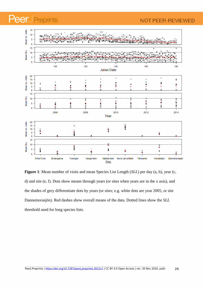
We calculated the length of the list of observed species for each visit (Species List Length;

SLL hereafter), later to be used as a measure of effort (Szabo et al. 2010). For computational

reasons, we restricted the maximum number of visits to 40 per day and site, prioritizing visits

with the longest species lists. SLLs ranged from 1 to 45 species. Around 60% of all visits

consisted of single observations (SLL = 1), although this proportion decreased over time (Fig.

1). In Figure S3 we compare the results of the model using the full dataset and only visits

with long species lists (SLL ≥ 10).

Seasonal site use model: Daily site occupancies using daily-based replicated observations

For each species, we use a dynamic state-space occupancy model (MacKenzie et al. 2006;

van Strien et al. 2013) to estimate daily occurrence status, adjusted for detection and

reporting probability (hereafter simply called detection probability). The occupancy model

consists of two sub-models coupled hierarchically: a process model (for the daily occurrence

status) and an observation model (for the stochasticity of species detections); the latter being

conditional on the process sub-model. In this way, each observation yj,d,t,i is modelled as

𝑦𝑗,𝑑,𝑡,𝑖 ~𝐵𝑒𝑟𝑛𝑜𝑢𝑙𝑙𝑖(𝑢𝑑,𝑡,𝑖×𝑝𝑗,𝑑,𝑡,𝑖) (eqn 1)

where ud,t,i is the (binary) occurrence status of the species in day d, year t and site i, and pj,d,t,i

is the detection probability of the species in each visit j, given that the species is present. The

occurrence status u depends on the occurrence probability ψ per day d, year t and site i

recursively through:

𝑢𝑑,𝑡,𝑖 ~𝐵𝑒𝑟𝑛𝑜𝑢𝑙𝑙𝑖(𝜓𝑑,𝑡,𝑖), (eqn 2)


8

𝜓𝑑,𝑡,𝑖 = 𝑢𝑑−1,𝑡,𝑖×𝜑𝑑−1,𝑡,𝑖 + (1 − 𝑢𝑑−1,𝑡,𝑖)×𝛾𝑑−1,𝑡,𝑖, (eqn 3)

Thus, whether site i that is occupied in day d-1 is still occupied in day d is determined by the

persistence probability (φ), whereas whether site i that is unoccupied in day d-1 is occupied

in day d depends on the colonization probability (γ). Because we expect persistence and

colonization probabilities to vary along the season, we further modelled these parameters as

𝑝𝑟𝑜𝑏𝑖𝑡(𝜑𝑑−1,𝑡,𝑖) = 𝑝𝐶𝑜𝑒𝑓1 + 𝑝𝐶𝑜𝑒𝑓2×𝐽𝐷𝑎𝑦𝑑−1 + 𝑝𝐶𝑜𝑒𝑓3×𝐽𝐷𝑎𝑦𝑑−12 + 휀𝑝𝐼𝑖 + 휀𝑝𝑇𝑡, (eqn 4)

𝑝𝑟𝑜𝑏𝑖𝑡(𝛾𝑑−1,𝑡,𝑖) = 𝑔𝐶𝑜𝑒𝑓1 + 𝑔𝐶𝑜𝑒𝑓2×𝐽𝐷𝑎𝑦𝑑−1 + 𝑔𝐶𝑜𝑒𝑓3×𝐽𝐷𝑎𝑦𝑑−12 + 휀𝑔𝐼𝑖 + 휀𝑔𝑇𝑡, (eqn 5)

where JDay is the Julian date. We modelled the effect of the Julian date as a quadratic

function to allow the colonization and persistence parameters to increase, decrease or both

within the season. In this way the model may be suitable for a wider range of species with

different phenology. We also added random effects for site (εpI and εgI) and year (εpT and

εgT) (see Appendix S1 for commented scripts).

The annual average use of site i by the focal species can be defined from the derived quantity

𝑧𝑡,𝑖 = (∑ 𝑢𝑑,𝑡,𝑖𝑛𝑑=1 ) 𝑛⁄ where n is the number of days during the season. In the same way, a

regional annual site use (Zt) can be defined as the average number of occurrence across all

days and sites.

The observation sub-model contains a detection probability p per visit j. Because we expected

detection to vary between visits, we modelled it as a saturation function of each visit’s SLL,

𝑝𝑗,𝑑,𝑡,𝑖 = 1 − 𝛿𝑡,𝑖 (𝑆𝐿𝐿𝑗,𝑑,𝑡,𝑖 + 𝛿𝑡,𝑖)⁄ , (eqn 6)

where δt,i is a real positive number defining the SLL required to obtain a detection probability

equal to 0.5 for a visit. Consequently, the shorter the list the lower the assumed observation

effort or the likelihood to report an observed species(Szabo et al. 2010; van Strien et al.

2013). With this function pj,d,t,i converges asymptotically to 1 as SLLj,d,t,i gets closer to ∞;


9

however, note that pj,d,t,i will be lower than 1 even when SLL is equal to the local species

richness. We further modelled δt,i as

log(𝛿𝑡,𝑖) = 𝑑𝐶𝑜𝑒𝑓1𝑖 + 𝑑𝐶𝑜𝑒𝑓2×𝑃𝐿𝐿𝑡, (eqn 7)

where dCoef1 is a site-specific parameter accounting for detectability varying among sites.

The variable PLLt is the proportion of long species lists (≥ 10 of the study species) over the

total number of lists each year among the nine sites (Fig. S2) and serves as a proxy to account

for potential non-linear changes in reporting behaviour among observers over time.

Preliminary results showed that this model cannot estimate variability in probability of

detection as a function of Julian date because it interfered with the estimation of the

persistence and colonization parameters in the occurrence sub-model. Therefore, detectability

is assumed to be constant within the season (see the Discussion section for pros and cons of

this model feature).

Annual site-occupancy model using within-season replication of observations

We also fitted a dynamic occupancy model to estimate annual occupancy probability (i.e.

using a closure period of 90 days; see e.g. van Strien et al. 2013), in order to directly compare

our results to previous methods adopted for opportunistic data. Given the abundance of

replicated visits we only used visits with SLL ≥ 10.

All models were fitted within the Bayesian framework using JAGS (Appendix S1; Plummer

2012). We chose conventional vague priors for all parameters, using Normal distributions

centred at zero and with standard deviation (SD) 1000 for effect parameters. We assumed

random effects to follow a Normal distribution centred at zero with independent standard

variation defined as σ = (1/τ)1/2 where τ is a precision parameter following a Gamma

distribution with shape and scale parameters equal 0.001. We used sufficient MCMC


10

iterations to achieve convergence of the models (burn-in = 5000, update = 15000). We used

95% quantiles as credible intervals to describe the precision of parameter estimates (Kéry

2010).

Goodness of fit through prediction

To investigate goodness-of-fit we checked if the model was able to reconstruct the original

data given the estimated parameter values (Gelman & Hill 2007; Kéry 2010; Chambert,

Rotella & Higgs 2014). To do so, we predicted observation events of a species given its

estimated daily occupancy status, and the effort spent in each visit. We summarized daily

observations (both observed and predicted data) into mean observed annual site use by

keeping the maximum detection status among the daily visits (1 if detected at least once

during the day, 0 otherwise) and averaging these values across the seasons (90 days) at each

site. We then graphically compared observed and predicted data of mean annual site use on a

1:1 discrepancy plot for all sites together.

We also evaluated goodness-of-fit of the models using site-specific Bayesian p-values, a.k.a.

“posterior predictive checks” (Kéry 2010; Chambert et al. 2014). Bayesian p-values quantify

the probability that the lack of fit of data replicated under the fitted model (i.e. data replicated

from the posterior distributions) is smaller than the lack of fit of the observed data. P-values

close to 0.5 indicate the model fits the data adequately and values close to 0 or to 1 indicate

under- or overfitting (Kéry 2010). The measure of discrepancy chosen in this case is the sums

of squares of differences (SSQ; eqn 8) between observed mean annual site use (𝑤𝑡,𝑖 =

(∑ max𝑗

𝑦𝑗,𝑑,𝑡,𝑖𝑛𝑑=1 ) 𝑛⁄ ; and w.newt,i for replicated data) and the model prediction of observed

mean annual site use (i.e. the average of the daily probabilities of detecting the species at

least once if present; �̅�𝑡,𝑖 = (∑ 𝑢𝑑,𝑡,𝑖×(1 − ∏ (1 − 𝑝𝑗,𝑑,𝑡,𝑖))𝑗𝑛𝑑=1 ) 𝑛⁄ ), as follow:


11

𝑆𝑆𝑄𝑖𝑜𝑏𝑠 = ∑ (𝑤𝑡,𝑖 − �̅�𝑡,𝑖)

2 (�̅�𝑡,𝑖 + 0.5)⁄𝑡 ;

𝑆𝑆𝑄𝑖𝑛𝑒𝑤 = ∑ (𝑤. 𝑛𝑒𝑤𝑡,𝑖 − �̅�𝑡,𝑖)

2 (�̅�𝑡,𝑖 + 0.5)⁄𝑡 , (eqn 8)

where 0.5 in the denominator is a correction for binomial variables to avoid dividing by

zeros.

Validation through simulations

We tested the assumptions and performance of our model under different scenarios by fitting

it to simulated data with known occurrence and sampling patterns. We simulated data using

the same sampling structure as for the real data, that is, daily replicates of visits during ten

90-day seasons at five sites, and using the observed increasing proportion of long lists

through time (PLLt, Fig. S2). The number of visits per day was drawn from a Poisson

distribution constrained at [1, 50] with expected value = 5 and site specific variability (see

Appendix S2). The length of each visits` species lists was randomly drawn according to the

observed proportion of single, short and long species lists (see Appendix S2 for more details).

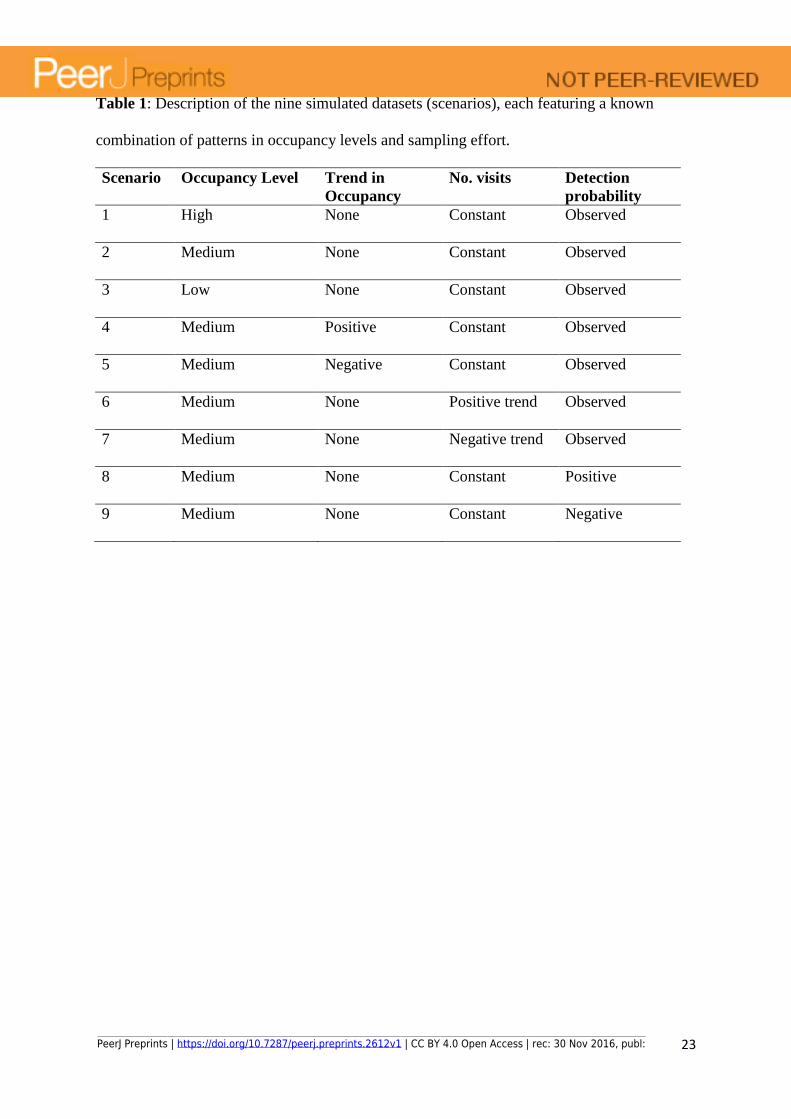
We fitted the model to nine simulated datasets partly mimicking patterns that are likely

observed in the opportunistic data (scenarios hereafter; Table 1), each featuring a known

combination of patterns in occupancy levels and effort that may influence model performance

but that are not explicitly accounted for in the model:

i) high, medium or low overall occupancy levels with variability among lakes in all

other parameters but stable occupancy through time;

ii) positive or negative trends over time on the persistence and colonization rates

iii) increasing or decreasing number of visits over time (maintaining the variability in

effort among sites)

iv) positive or negative trends in detection (and reporting) probabilities, on top of the

observed trend in PLLt that is common to all scenarios.


12

For more details about the simulation procedure and parameters settings, read Appendix

S2. We evaluated the goodness-of-fit of the models in the same way as described above,

and the ability of the models to estimate the known occurrence data.

Results

Analyses with real data on wetland birds

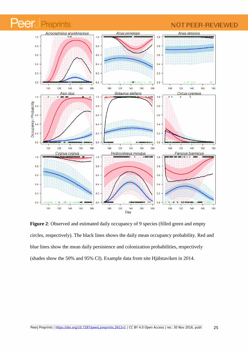
The model estimates daily occupancy statuses by correcting for false absences based on each

day’s effort (both number of visits and each visit’s SLL) and on the assumed species

colonization/extinction dynamics at a site and year (Fig. 2). Estimated mean annual site use

(summarised from estimated daily occupancy status) varies from year to year, displaying

large between-year changes for some species (Fig. 3, exemplified with nine selected bird

species). Estimates of occupancy probability were in general precise (i.e. small credible

intervals) even for rare species, as long as some of the sites were well sampled (i.e. enough to

confidently separate occupancy and detection probabilities) and if the species occurred

regularly at those sites (i.e. consistently during the same periods across all years it was

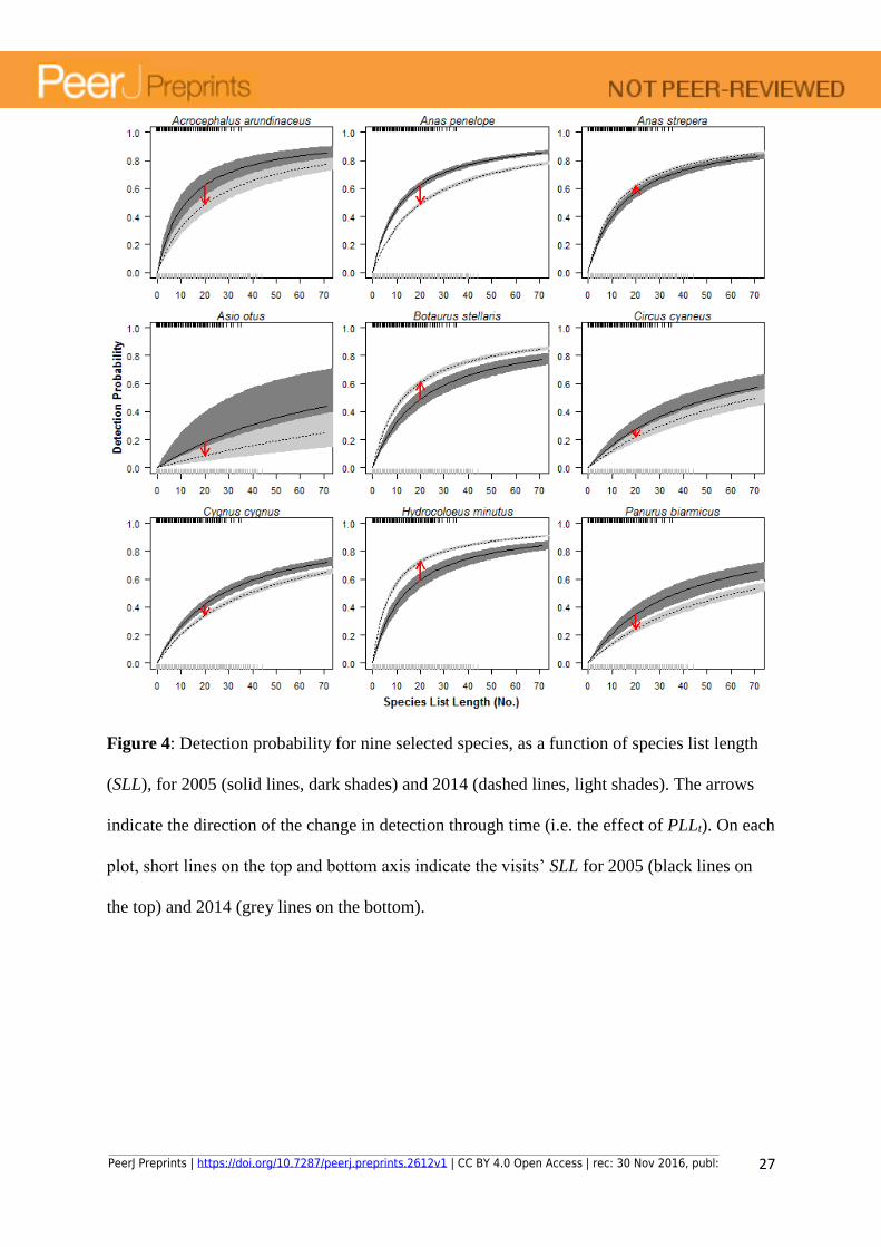
present; e.g. Asio otus). The probability of detection depended on the visits’ SLL and on the

proportion of long lists, PLLt. Estimates of the probability of detection were less precise for

species with lower site use (Fig. 4). We observed low discrepancy between observations and

predicted observations of mean annual site use, and no systematic bias was observed for 64

out of 71 investigated species (Appendix S3). However, deviations from the 1:1 line between

observations and expectations (to either side) were noted for seven species with anecdotic

occurrences in some sites. Bayesian p-values (posterior predictive checks) were useful to

corroborate if the observed local daily dynamics adjust to the overall daily dynamics

estimated from all sites. Bad fit was then only observed on individual sites with little data

were the local dynamics does not match the dynamics observed in other sites (Appendix S3).


13

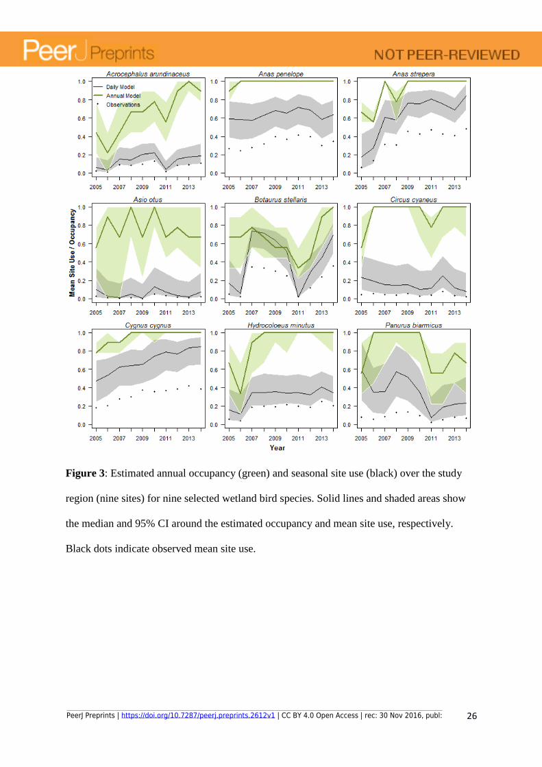
Comparing patterns of dynamics from the seasonal site use vs. the annual occupancy model

Using the visits with long species list we calculated the corresponding annual occupancy over

the nine wetlands between 2005 and 2014. Although annual occupancy levels are generally

higher than the mean site use, they frequently display a similar broad pattern of temporal

dynamics (Fig. 3). However, for some more common or widespread species the annual

occupancy model often displayed no temporal variation in occupancy, as all sites were

determined occupied in all years (e.g. A. penelope and C. cyaneus, and C. cygnus and H.

minutus after 2008, Fig. 3). By contrast, for some of these species the site use model

suggested a positive trend (C. cygnus) or a possible negative trend (C. cyaneus) in site use.

Similarly, large differences between annual occupancy and mean site use as estimated by the

annual vs. daily occupancy models respectively, show that the annual model fails to handle

the effects of temporary visits by over-estimating the species annual occupancy during the

breeding season (see Discussion for an example).

Validation of the seasonal site use model by simulated data

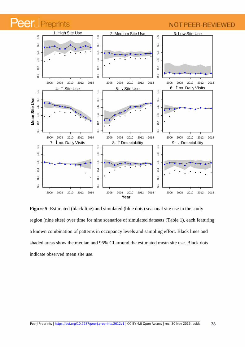
The daily occupancy model gave accurate and robust estimates of annual site use for the

simulated data regardless of the mean site use level (i.e. number of days present in any site in

the region; Scenarios 1, 2 and 3), and trends in occupancy (Scenarios 4 and 5), number of

visits (Scenarios 6 and 7) or in detectability (Scenarios 8 and 9). Most of the simulated yearly

site use data points were overlapping with the site use values estimated from the model (i.e.

all simulated points were within the 95% CI, but mostly close to the median of the estimates)

across all scenarios (Fig. 5).


14

The model uncertainty (95% CI), however, depends on the combined effect of number of

daily visits and each visit’s SLL, but also on the mean site use level (i.e. number of days

present at the site).When mean site use level is very low (Scenario 3), there are too few

detections to inform the model, which becomes less accurate and less precise at estimating

the probabilities of detection and the colonization/extinction probabilities (Fig. 5, Scenario 3).

This results in high uncertainties unless the sampling effort is high enough to detect every

presence of the species.

The model estimated temporal trends in site use regardless of trends in number of

observations per day (Scenarios 4 and 5). As expected, model uncertainty is higher the lower

the number of visits per day (Scenarios 6 and 7) and the lower the species detectability

(Scenarios 8 and 9). Regardless of the probability of detection, the higher the number of visits

per day the more likely the species is detected if present. Therefore, the higher the number of

visits per day, the smaller the discrepancy between observations and the occupancy status of

the species (Scenario 6). Alternatively, even accounting for an increase in PLLt in all visits,

detections are not guaranteed if the number of visits are too few (Scenario 7). Despite an

increase in model uncertainty, the model correctly estimated the occurrence status of the

species under both changing number of visits and changing species detectability.

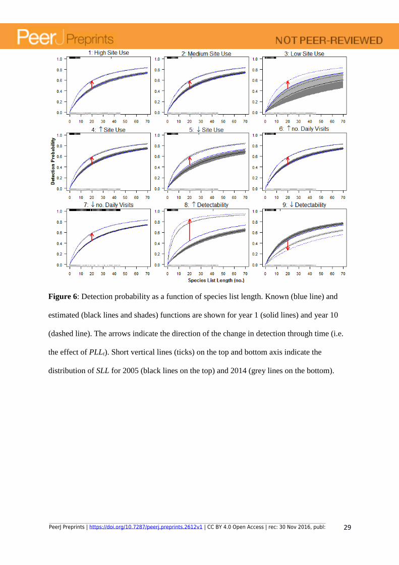
The model identifies changes in detectability independently of the trends in number of visits

and PLLt. Despite the observed increase in proportion of long lists (PLLt, Fig. 1 and Fig. S2)

is included in the model as a time-dependent variable affecting the probability of detection,

the model also adjusts the effect parameter for PLLt to non-observed changes in detectability

(Scenarios 8 and 9, Figs. 5 and red arrows in Fig. 6). That is, even when the proportion of

long lists among visits is high (high PLLt), detectability can naturally decrease due to e.g.


15

change in habitat conditions. However, for the simulated data the model is able to correct for

this trend and estimates of occupancy are not affected.

Discussion

We estimate the daily probability of occupancy at sites and the average site use during each

breeding season for wetland birds, including migratory species that may display strong

seasonal dynamics depending on the timing of arrival and departure from breeding areas. We

use dynamic occupancy models within seasons by narrowing the time window traditionally

used from a year or season to a single day. We achieve this by making use of opportunistic

citizen science data that contain multiple visits made by different observers at a site within a

day. The two occupancy model variants (annual- and daily-based) summarize different

aspects of the species dynamics in the study area. While the annual occupancy model used so

far inform us about the proportion of sites in which we can expect a species to be present at

some point during the season, the seasonal site use model informs us about the proportion of

days each site is likely to be used. Although there are similarities between yearly summaries

of both models (Fig. 3), the seasonal site use model make opportunistic data available to

answer new questions and investigate within-season dynamics. As an example, one could

study phenology of arrival and departure (Fig. 2), and actual site use to potentially separate

temporary occurrences, e.g. by migrants and prospectors, from those linked to breeding

activities. Furthermore, model validation based on simulated data suggests that the

performance of the seasonal site use model in terms of capturing the species mean site use

over time is robust to underlying variability and trends in effort and species detectability.


16

Seasonal site use vs. annual occupancy models

Previous annual occupancy models have typically used the breeding season (e.g. two-three

months) as the time window to estimate annual occupancy at sites (e.g. 1 km2 grid squares)

(Royle & Kéry 2007; Royle & Dorazio 2008; van Strien et al. 2013; Isaac et al. 2014).

However, using such long time window may likely violate the assumption of closure for

mobile species with within-season dynamics, thus potentially reducing estimates of

probability of detection and increase the uncertainty of occupancy estimates (MacKenzie et

al. 2003). For example, when the aim is to analyse occurrences of breeding species, an annual

occupancy model will over-estimate site use of species with temporary occurrences (e.g.

migrants passing by, single itinerary prospecting individuals) as even a single observation

during the closure period will be viewed as an occupancy. On the other hand, an occupancy

model with within-season dynamics, such as our seasonal site use model will produce

estimates of the extent to which sites are actually used. Two illustrative examples are the little

gull (H. minutus) and the hen harrier (Circus cyaneus) which we know from careful

observations made by the local ornithological society attempted to breed in only three and

none of the nine wetlands, respectively, during 2005 to 2014 (Annual birds reports from the

Ornithological Society of Uppland 2005-2014). These species regularly stop-over at these

wetlands on their way to their breeding areas in northern Sweden and Finland, being

frequently observed for several days during spring and early summer. The annual model

therefore suggests an occupancy probability close to one for most years for this species (Fig.

3). The seasonal site use model, on the other hand, suggest a relatively low site use. In this

way, the site use model may be used to detect these passages of migrants thus enabling a

separation between potential breeders and migrants or vagrants (Fig. 3 and Appendix S3).

Furthermore, as individuals may move in and out of the sites during the study period, daily

occupancy of a site may indicate how site use is changing during the season. In this way such


17

a seasonal site use model may also be able to estimate the relative importance of different

sub-localities as foraging or stop-over sites in a network of e.g. wetland sites.

Opportunistic data at frequently visited sites offer good opportunities to narrow the time

window of the closure period because of the large amount of data at specific sites. Several of

the localities in our study, which include popular birding wetlands with observation towers,

were visited two or more times per day by different observers during the spring 2005-2014.

In general, the span of the within season closure period of our model may be optimized to the

data at hand. If, for instance, multiple visits to sites are common on a weekly but not on a

daily basis, a closure period of one week might be used instead.

Opportunistic data and the robustness of the seasonal site use model

The probability of at least one reported observation of a species at a site on a particular day is

the result of a combination between the probability of detection of each visit, and the number

of visits made. The probability of detection during each visit depends on effort allocated to

observing species and the willingness to report them if seen. SLL is an established surrogate

for the effort of a visit in opportunistic data (Szabo et al. 2010; van Strien et al. 2013; Barnes

et al. 2015). Even though detection probability and willingness to report an observation differ

largely among species, it is expected that the longer the SLL the lower the chance of

deliberately leaving species out of the report (van Strien et al. 2013). However, even “low-

quality” observations (e.g. SLL = 1) may be informative for the occupancy status of the few

species that are on such a list. If there are sufficient visits reporting only one or a few species

they can be useful for estimating occupancy (e.g. beginning of Scenario 7, where plenty of

visits each with very short species lists are enough to precisely estimate the mean site use).

Therefore, as an alternative to the seminal species list comparison approach proposed by


18

Szabo et al. (2010) where short species list were omitted, we also make use of even single

(incidental) observations that have often been regarded as containing little information

(Szabo et al. 2010; Isaac & Pocock 2015). This addition does not add noise but rather

improves precision in estimates of daily occupancy and mean site use of rare species (Fig.

S3).

In our site use model, detectability is assumed to be site- and year-specific but constant

within the season. This is because trying to estimate daily variations in detectability would

interfere with the estimation of the daily persistence and colonization parameters in the

occurrence sub-model. However, because the probability of detection is determined by each

visit’s SLL that varies among visits and may decrease along the season (Strebel et al. 2014),

the model implicitly allows for some variation in the probability of detection within the

season. Alternatively, in case there are good reasons to believe that detectability changes

during the breeding season (e.g. due to increased cryptic behaviour) a change in detectability

between intermediate time windows (e.g. months) could be parameterized and tested with this

model by adding a time covariate to Equation 7 (see methods).

The seasonal site use model presented here accounts for effects of changes in the behaviour

of observers over time on species detectability, using the overall proportion of species lists

longer than 10 (PLLt) as a proxy. Specifically, PLLt captures a non-linear increase in the

proportion of visits with long lists during the first few years in the data analysed here,

suggesting that the overall quality of reports may have increased. The effect of PLLt was,

however, negative for some species (red arrows in Fig. 4) indicating that observers are

decreasingly reporting certain species despite an overall change towards longer lists. This

may suggest a negative trend in the species abundance that is not reflected in the species


19

occupancy. Alternative proxies, such as temporal trend, could also be used to adjust for

changes in reporting behaviour over time, although when tested in this study the model did

not converge into a solution.

In addition to the assumption that species list length serves as a reasonable proxy for

sampling effort, site-occupancy models of opportunistic data rely on additional assumptions.

For example, a general assumption of site-occupancy models is that reports from different

visits are independent, which may not be the case if observers share their sightings. Despite

estimates of site use being robust to the deviations explored in the simulated scenarios, there

is thus no guarantee that the model correctly adjusts for variation in effort, observer

behaviour and observer willingness to report a species. Unfortunately, no further conclusion

can be drawn without validation against systematically collected data. Currently, little is

known about variations in observer behaviours and the decisions underlying whether

observations are reported or not. Some studies comparing analyses of opportunistic data

against survey data do suggest that occupancy models may handle the most serious causes of

bias (van Strien et al. 2013; Isaac et al. 2014), while other studies suggest a poor fit between

opportunistic and survey data (Kamp et al. 2016).

In conclusion, by making use of dense opportunistic data at popular localities we could

markedly reduce the time interval for the closure criterion (here to one day periods) and get

repeated estimates of occupancy within a pre-defined time period (here the breeding season

of three months) to estimate: (i) daily site occupancy and (ii) site use during the breeding

season (here mean number of days a species is present at a site) in contrast to a binary

variable produced by an annual occupancy model, and hence (iii) the possibility to redefine

the criteria for counting a species as present at a site based on its activity within the season.


20

Furthermore, the seasonal site use model has the potential to estimate the relative importance

of each site in a wetland network in terms of site use.

Data Accessibility

Species daily observations: We intend to archive the original data on Dryad, but it could also

be obtained from www.artportalen.se at any time.

Acknowledgements

We are thankful to Guillaume Chapron for useful comments on the manuscript and to

Frederik Barraquand for fruitful discussions at early stages of this work. The research was

financially supported by the Swedish Research Council VR (J. K.) and FORMAS (T. P.).

Literature Cited

Barnes, M., Szabo, J.K., Morris, W.K. & Possingham, H. (2015) Evaluating protected area effectiveness using bird lists in the Australian Wet Tropics. Diversity and Distributions, 21, 368–378.

Boyce, M.S. & McDonald, L.L. (1999) Relating populations to habitats using resource selection functions. Trends in Ecology & Evolution, 14, 268–272.

Chambert, T., Rotella, J.J. & Higgs, M.D. (2014) Use of posterior predictive checks as an inferential tool for investigating individual heterogeneity in animal population vital rates. Ecology and Evolution, 4, 1389–1397.

Cruickshank, S.S., Ozgul, A., Zumbach, S. & Schmidt, B.R. (2016) Quantifying population declines based on presence-only records for red-list assessments. Conservation Biology, 30, 1112–1121.

Fernández, D. & Nakamura, M. (2015) Estimation of spatial sampling effort based on presence-only data and accessibility. Ecological Modelling, 299, 147–155.

Gelman, A. & Hill, J. (2007) Data Analysis Using Regression and Multilevel/hierarchical Models. Cambridge University Press Cambridge, New York, USA.


http://www.artportalen.se/

21

Graham, C.H., Ferrier, S., Huettman, F., Moritz, C. & Peterson, A.T. (2004) New developments in museum-based informatics and applications in biodiversity analysis. Trends in Ecology & Evolution, 19, 497–503.

Hanski, I. (1999) Metapopulation Ecology. Oxford University Press, Oxford, UK.

Isaac, N.J.B. & Pocock, M.J.O. (2015) Bias and information in biological records. Biological Journal of the Linnean Society, 115, 522–531.

Isaac, N.J.B., van Strien, A.J., August, T.A., de Zeeuw, M.P. & Roy, D.B. (2014) Statistics for citizen science: extracting signals of change from noisy ecological data. Methods in Ecology and Evolution, 5, 1052–1060.

Jeppsson, T., Lindhe, A., Gärdenfors, U. & Forslund, P. (2010) The use of historical collections to estimate population trends: A case study using Swedish longhorn beetles (Coleoptera: Cerambycidae). Biological Conservation, 143, 1940–1950.

Kamp, J., Oppel, S., Heldbjerg, H., Nyegaard, T. & Donald, P.F. (2016) Unstructured citizen science data fail to detect long-term population declines of common birds in Denmark. Diversity and Distributions, n/a-n/a.

Kendall, W.L., Hines, J.E., Nichols, J.D. & Grant, E.H.C. (2013) Relaxing the closure assumption in occupancy models: staggered arrival and departure times. Ecology, 94, 610–617.

Kéry, M. (2010) Introduction to WinBUGS for Ecologists, 1st edition. Academic Press, Amsterdam.

Kéry, M., Gardner, B. & Monnerat, C. (2010) Predicting species distributions from checklist data using site-occupancy models. Journal of Biogeography, 37, 1851–1862.

Lukyanenko, R., Parsons, J. & Wiersma, Y.F. (2016) Emerging problems of data quality in citizen science. Conservation Biology, 30, 447–449.

MacKenzie, D.I., Nichols, J.D., Hines, J.E., Knutson, M.G. & Franklin, A.B. (2003) Estimating site occupancy, colonization, and local extinction when a species is detected imperfectly. Ecology, 84, 2200–2207.

MacKenzie, D.I., Nichols, J.D., Royle, J.A., Pollock, K.H., Bailey, L.L. & Hines, J.E. (2006) Occupancy Estimation and Modeling: Inferring Patterns and Dynamics of Species Occurrence. Academic Press, London, UK.

Mair, L. & Ruete, A. (2016) Explaining spatial variation in the recording effort of citizen science data across multiple taxa. PLOS ONE, 11, e0147796.

Plummer, M. (2012) JAGS: A Program for Analysis of Bayesian Graphical Models Using Gibbs Sampling.

Roth, T., Strebel, N. & Amrhein, V. (2014) Estimating unbiased phenological trends by adapting site-occupancy models. Ecology, 95, 2144–2154.

Royle, J.A. & Dorazio, R.M. (2008) Hierarchical Modeling and Inference in Ecology: The Analysis of Data from Populations, Metapopulations and Communities. Academic Press, Amsterdam.


22

Royle, J.A. & Kéry, M. (2007) A bayesian state-space formulation of dynamic occupancy models. Ecology, 88, 1813–1823.

Snäll, T., Forslund, P., Jeppsson, T., Lindhe, A. & O’Hara, R.B. (2014) Evaluating temporal variation in Citizen Science Data against temporal variation in the environment. Ecography, 37, 293–300.

Snäll, T., Kindvall, O., Nilsson, J. & Pärt, T. (2011) Evaluating citizen-based presence data for bird monitoring. Biological Conservation, 144, 804–810.

Strebel, N., Kéry, M., Schaub, M. & Schmid, H. (2014) Studying phenology by flexible modelling of seasonal detectability peaks. Methods in Ecology and Evolution, 5, 483–490.

van Strien, A.J., van Swaay, C.A.M. & Termaat, T. (2013) Opportunistic citizen science data of animal species produce reliable estimates of distribution trends if analysed with occupancy models. Journal of Applied Ecology, 50, 1450–1458.

van Strien, A.J., Termaat, T., Groenendijk, D., Mensing, V. & Kéry, M. (2010) Site-occupancy models may offer new opportunities for dragonfly monitoring based on daily species lists. Basic and Applied Ecology, 11, 495–503.

Suarez, A.V. & Tsutsui, N.D. (2004) The value of museum collections for research and society. BioScience, 54, 66–74.

Szabo, J.K., Vesk, P.A., Baxter, P.W.J. & Possingham, H.P. (2010) Regional avian species declines estimated from volunteer-collected long-term data using List Length Analysis. Ecological Applications, 20, 2157–2169.


23

Table 1: Description of the nine simulated datasets (scenarios), each featuring a known

combination of patterns in occupancy levels and sampling effort.

Scenario Occupancy Level Trend in

Occupancy

No. visits Detection

probability

1 High None Constant Observed

2 Medium None Constant Observed

3 Low None Constant Observed

4 Medium Positive Constant Observed

5 Medium Negative Constant Observed

6 Medium None Positive trend Observed

7 Medium None Negative trend Observed

8 Medium None Constant Positive

9 Medium None Constant Negative


24

Figure 1: Mean number of visits and mean Species List Length (SLL) per day (a, b), year (c,

d) and site (e, f). Dots show means through years (or sites when years are in the x axis), and

the shades of grey differentiate dots by years (or sites; e.g. white dots are year 2005, or site

Dannemorasjön). Red dashes show overall means of the data. Dotted lines show the SLL

threshold used for long species lists.


25

Figure 2: Observed and estimated daily occupancy of 9 species (filled green and empty

circles, respectively). The black lines shows the daily mean occupancy probability. Red and

blue lines show the mean daily persistence and colonization probabilities, respectively

(shades show the 50% and 95% CI). Example data from site Hjälstaviken in 2014.


26

Figure 3: Estimated annual occupancy (green) and seasonal site use (black) over the study

region (nine sites) for nine selected wetland bird species. Solid lines and shaded areas show

the median and 95% CI around the estimated occupancy and mean site use, respectively.

Black dots indicate observed mean site use.


27

Figure 4: Detection probability for nine selected species, as a function of species list length

(SLL), for 2005 (solid lines, dark shades) and 2014 (dashed lines, light shades). The arrows

indicate the direction of the change in detection through time (i.e. the effect of PLLt). On each

plot, short lines on the top and bottom axis indicate the visits’ SLL for 2005 (black lines on

the top) and 2014 (grey lines on the bottom).


28

Figure 5: Estimated (black line) and simulated (blue dots) seasonal site use in the study

region (nine sites) over time for nine scenarios of simulated datasets (Table 1), each featuring

a known combination of patterns in occupancy levels and sampling effort. Black lines and

shaded areas show the median and 95% CI around the estimated mean site use. Black dots

indicate observed mean site use.

2006 2008 2010 2012 2014

0.0

0.2

0.4

0.6

0.8

1.0

1: High Site Use

2006 2008 2010 2012 2014

0.0

0.2

0.4

0.6

0.8

1.0

2: Medium Site Use

2006 2008 2010 2012 2014

0.0

0.2

0.4

0.6

0.8

1.0

3: Low Site Use

2006 2008 2010 2012 2014

0.0

0.2

0.4

0.6

0.8

1.0

4: Site Use

Me

an

Sit

e U

se

2006 2008 2010 2012 2014

0.0

0.2

0.4

0.6

0.8

1.0

5: Site Use

2006 2008 2010 2012 2014

0.0

0.2

0.4

0.6

0.8

1.0

6: no. Daily Visits

2006 2008 2010 2012 2014

0.0

0.2

0.4

0.6

0.8

1.0

7: no. Daily Visits

2006 2008 2010 2012 2014

0.0

0.2

0.4

0.6

0.8

1.0

8: Detectability

Year

2006 2008 2010 2012 2014

0.0

0.2

0.4

0.6

0.8

1.0

9: Detectability


29

Figure 6: Detection probability as a function of species list length. Known (blue line) and

estimated (black lines and shades) functions are shown for year 1 (solid lines) and year 10

(dashed line). The arrows indicate the direction of the change in detection through time (i.e.

the effect of PLLt). Short vertical lines (ticks) on the top and bottom axis indicate the

distribution of SLL for 2005 (black lines on the top) and 2014 (grey lines on the bottom).


Exploiting opportunistic observations to estimate changes ... · PDF fileExploiting...

Documents

Transcript of Exploiting opportunistic observations to estimate changes ... · PDF fileExploiting...