Opportunistic Physical Design for Big Data Analytics

Jeff LeFevre+†

Jagan Sankaranarayanan∗ Hakan Hacıgümüs∗

Junichi Tatemura∗ Neoklis Polyzotis+ Michael J. Carey%

∗NEC Labs America, Cupertino, CA +University of California, Santa Cruz %University of California, Irvine

{jlefevre,alkis}@cs.ucsc.edu, {jagan,hakan,tatemura}@nec-labs.com, mjcarey@ics.uci.edu

ABSTRACTBig data analytical systems, such as MapReduce, perform aggressivematerialization of intermediate job results in order to support fault tol-erance. When jobs correspond to exploratory queries submitted bydata analysts, these materializations yield a large set of materializedviews that we propose to treat as an opportunistic physical design.We present a semantic model for UDFs that enables effective reuseof views containing UDFs along with a rewrite algorithm that prov-ably finds the minimum-cost rewrite under certain assumptions. Anexperimental study on real-world datasets using our prototype basedon Hive shows that our approach can result in dramatic performanceimprovements.

1. INTRODUCTIONData analysts have the crucial task of analyzing the ever increasing

volume of data that modern organizations collect in order to produceactionable insights. As expected, this type of analysis on big datais highly exploratory in nature and involves an iterative process: thedata analyst starts with an initial query over the data, examines theresults, then reformulates the query and may even bring in additionaldata sources, and so on [9]. Typically, these queries involve sophis-ticated, domain-specific operations that are linked to the type of dataand the purpose of the analysis, e.g., performing sentiment analysisover tweets or computing network influence. Because a query is oftenrevised multiple times in this scenario, there can be significant overlapbetween queries. There is an opportunity to speed up these explo-rations by reusing previous query results either from the same analystor from different analysts performing a related task.

MapReduce (MR) has become a de-facto tool for this type of anal-ysis. It offers scalability to large datasets, easy incorporation of newdata sources, the ability to query right away without defining a schemaup front, and extensibility through user-defined functions (UDFs). An-alyst queries are often written in a declarative query language, e.g.,HiveQL or PigLatin, which are automatically translated to a set ofMR jobs. Each MR job involves the materialization of intermediateresults (the output of mappers, the input of reducers and the output ofreducers) for the purpose of failure recovery. A typical Hive or Pigquery will spawn a multi-stage job that will involve several such ma-

†Work done when the author was at NEC Labs America

Permission to make digital or hard copies of all or part of this work for personal or class-room use is granted without fee provided that copies are not made or distributed for profitor commercial advantage and that copies bear this notice and the full citation on the firstpage. Copyrights for components of this work owned by others than ACM must be hon-ored. Abstracting with credit is permitted. To copy otherwise, or republish, to post onservers or to redistribute to lists, requires prior specific permission and/or a fee. Requestpermissions from permissions@acm.org.SIGMOD’14, June 22–27, 2014, Snowbird, UT, USA.Copyright is held by the owner/author(s). Publication rights licensed to ACM.ACM 978-1-4503-2376-5/14/06 ...$15.00.http://dx.doi.org/10.1145/2588555.2610512 .

terializations. We refer to these execution artifacts as opportunisticmaterialized views.

We propose to treat these views as an opportunistic physical de-sign and to use them to rewrite queries. The opportunistic nature ofour technique has several nice properties: the materialized views aregenerated as a by-product of query execution, i.e., without additionaloverhead; the set of views is naturally tailored to the current work-load; and, given that large-scale analysis systems typically execute alarge number of queries, it follows that there will be an equally largenumber of materialized views and hence a good chance of finding agood rewrite for a new query. Our results indicate the savings in queryexecution time can be dramatic: a rewrite can reduce execution timeby up to an order of magnitude.

Rewriting a query using views in the context of MR involves aunique combination of technical challenges that distinguish it from thetraditional problem of query rewriting. First, the queries and viewsalmost certainly contain UDFs, thus query rewriting requires somesemantic understanding of UDFs. These MR UDFs for big data anal-ysis are composed of arbitrary user-code and may involve a sequenceof MR jobs. Second, any query rewriting algorithm that can utilizeUDFs now has to contend with a potentially large number of opera-tors since any UDF can be included in the rewriting process. Third,there can be a large search space of views to consider for rewriting dueto the large number of materialized views in the opportunistic physicaldesign, since they are almost free to retain (storage permitting).

Recent methods to reuse MR computations such as ReStore [6] andMRShare [21] lack any semantic understanding of execution artifactsand can only reuse/share cached results when execution plans are syn-tactically identical. We strongly believe that any truly effective so-lution will have to a incorporate a deeper semantic understanding ofcached results and “look into” the UDFs as well.

Contributions. In this paper we present a novel query-rewrite algo-rithm that targets the scenario of opportunistic materialized views in anMR system with queries that contain UDFs. We propose a UDF modelthat has a limited semantic understanding of UDFs, yet enables effec-tive reuse of previous results. Our rewrite algorithm employs tech-niques inspired by spatial databases (specifically, nearest-neighborsearches in metric spaces [12]) in order to provide a cost-based in-cremental enumeration of the huge space of candidate rewrites, gen-erating the optimal rewrite in an efficient manner. Specifically, ourcontributions can be summarized as follows:• A gray-box UDF model that is simple but expressive enough to

capture a large class of MR UDFs that includes many commonanalysis tasks. The UDF model further provides a quick way tocompute a lower-bound on the cost of a potential rewrite givenjust the query and view definitions. We provide the model and thetypes of UDFs it admits in Sections 3–4.

• A rewriting algorithm that uses the lower-bound to (a) graduallyexplode the space of rewrites as needed, and (b) only attempts arewrite for those views with good potential to produce a low-cost

MATERIALIZED  VIEW  METADATA  STORE  

EXECUTION  ENGINE  

OPTIMIZER  

REWRITER  

Rewrites

Plan

ANALYST  

ANALYST  

ANALYST  

q Plan, Cost

Base Data & Materialized Views

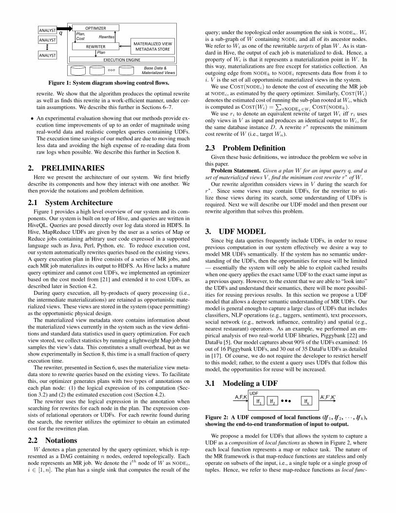
Figure 1: System diagram showing control flows.

rewrite. We show that the algorithm produces the optimal rewriteas well as finds this rewrite in a work-efficient manner, under cer-tain assumptions. We describe this further in Sections 6–7.

• An experimental evaluation showing that our methods provide ex-ecution time improvements of up to an order of magnitude usingreal-world data and realistic complex queries containing UDFs.The execution time savings of our method are due to moving muchless data and avoiding the high expense of re-reading data fromraw logs when possible. We describe this further in Section 8.

2. PRELIMINARIESHere we present the architecture of our system. We first briefly

describe its components and how they interact with one another. Wethen provide the notations and problem definition.

2.1 System ArchitectureFigure 1 provides a high level overview of our system and its com-

ponents. Our system is built on top of Hive, and queries are written inHiveQL. Queries are posed directly over log data stored in HDFS. InHive, MapReduce UDFs are given by the user as a series of Map orReduce jobs containing arbitrary user code expressed in a supportedlanguage such as Java, Perl, Python, etc. To reduce execution cost,our system automatically rewrites queries based on the existing views.A query execution plan in Hive consists of a series of MR jobs, andeach MR job materializes its output to HDFS. As Hive lacks a maturequery optimizer and cannot cost UDFs, we implemented an optimizerbased on the cost model from [21] and extended it to cost UDFs, asdescribed later in Section 4.2.

During query execution, all by-products of query processing (i.e.,the intermediate materializations) are retained as opportunistic mate-rialized views. These views are stored in the system (space permitting)as the opportunistic physical design.

The materialized view metadata store contains information aboutthe materialized views currently in the system such as the view defini-tions and standard data statistics used in query optimization. For eachview stored, we collect statistics by running a lightweight Map job thatsamples the view’s data. This constitutes a small overhead, but as weshow experimentally in Section 8, this time is a small fraction of queryexecution time.

The rewriter, presented in Section 6, uses the materialize view meta-data store to rewrite queries based on the existing views. To facilitatethis, our optimizer generates plans with two types of annotations oneach plan node: (1) the logical expression of its computation (Sec-tion 3.2) and (2) the estimated execution cost (Section 4.2).

The rewriter uses the logical expression in the annotation whensearching for rewrites for each node in the plan. The expression con-sists of relational operators or UDFs. For each rewrite found duringthe search, the rewriter utilizes the optimizer to obtain an estimatedcost for the rewritten plan.

2.2 NotationsW denotes a plan generated by the query optimizer, which is rep-

resented as a DAG containing n nodes, ordered topologically. Eachnode represents an MR job. We denote the ith node of W as NODEi,i ∈ [1, n]. The plan has a single sink that computes the result of the

query; under the topological order assumption the sink is NODEn. Wi

is a sub-graph of W containing NODEi and all of its ancestor nodes.We refer to Wi as one of the rewritable targets of plan W . As is stan-dard in Hive, the output of each job is materialized to disk. Hence, aproperty of Wi is that it represents a materialization point in W . Inthis way, materializations are free except for statistics collection. Anoutgoing edge from NODEk to NODEi represents data flow from k toi. V is the set of all opportunistic materialized views in the system.

We use COST(NODEi) to denote the cost of executing the MR jobat NODEi, as estimated by the query optimizer. Similarly, COST(Wi)denotes the estimated cost of running the sub-plan rooted at Wi, whichis computed as COST(Wi) =

∑∀NODEk∈Wi

COST(NODEk).We use ri to denote an equivalent rewrite of target Wi iff ri uses

only views in V as input and produces an identical output to Wi, forthe same database instance D. A rewrite r∗ represents the minimumcost rewrite of W (i.e., target Wn).

2.3 Problem DefinitionGiven these basic definitions, we introduce the problem we solve in

this paper.Problem Statement. Given a plan W for an input query q, and a

set of materialized views V , find the minimum cost rewrite r∗ of W .Our rewrite algorithm considers views in V during the search for

r∗. Since some views may contain UDFs, for the rewriter to uti-lize those views during its search, some understanding of UDFs isrequired. Next we will describe our UDF model and then present ourrewrite algorithm that solves this problem.

3. UDF MODELSince big data queries frequently include UDFs, in order to reuse

previous computation in our system effectively we desire a way tomodel MR UDFs semantically. If the system has no semantic under-standing of the UDFs, then the opportunities for reuse will be limited— essentially the system will only be able to exploit cached resultswhen one query applies the exact same UDF to the exact same input asa previous query. However, to the extent that we are able to “look into”the UDFs and understand their semantics, there will be more possibil-ities for reusing previous results. In this section we propose a UDFmodel that allows a deeper semantic understanding of MR UDFs. Ourmodel is general enough to capture a large class of UDFs that includesclassifiers, NLP operations (e.g., taggers, sentiment), text processors,social network (e.g., network influence, centrality) and spatial (e.g.,nearest restaurant) operators. As an example, we performed an em-pirical analysis of two real-world UDF libraries, Piggybank [22] andDataFu [5]. Our model captures about 90% of the UDFs examined: 16out of 16 Piggybank UDFs, and 30 out of 35 DataFu UDFs as detailedin [17]. Of course, we do not require the developer to restrict herselfto this model; rather, to the extent a query uses UDFs that follow thismodel, the opportunities for reuse will be increased.

3.1 Modeling a UDF

lf2  lf1   lfk  

UDF A,F,K A’,F’,K’

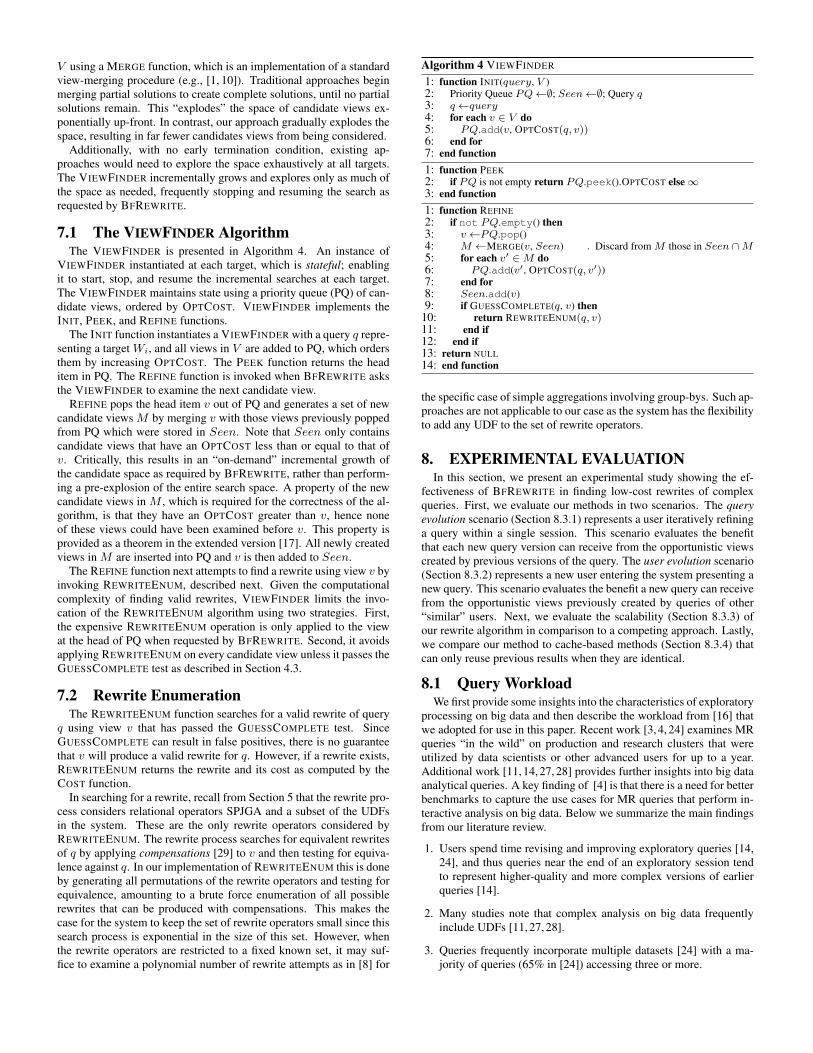
Figure 2: A UDF composed of local functions (lf1, lf2, · · · , lfk),showing the end-to-end transformation of input to output.

We propose a model for UDFs that allows the system to capture aUDF as a composition of local functions as shown in Figure 2, whereeach local function represents a map or reduce task. The nature ofthe MR framework is that map-reduce functions are stateless and onlyoperate on subsets of the input, i.e., a single tuple or a single group oftuples. Hence, we refer to these map-reduce functions as local func-

tions. A local function can only perform a combination of the follow-ing three types of operations performed by map and reduce tasks.1. Discard or add attributes, where an added attribute and its values

may be determined by arbitrary user code

2. Discard tuples by applying filters, where the filter predicates maybe performed by arbitrary user code

3. Perform grouping of tuples on a common key, where the groupingoperation may be performed by arbitrary user code

The end-to-end transformation of a UDF is obtained by compos-ing the operations performed by each local function lf in the UDF.Our model captures the fine-grain dependencies between the input andoutput tuples in the following way.

The UDF input is modeled as (A,F,K) where A is the set of at-tributes, F is set of filters previously applied to the input, and Kis the current grouping of the input, which captures the keys of thedata. The output is modeled as (A′, F ′,K′) with the same semantics.Our model describes a UDF as the transformation from (A,F,K) to(A′, F ′,K′) as performed by a composition of local functions usingoperation types (1) (2) (3) above. Figure 2 shows how to semanticallymodel a UDF that takes any arbitrary input represented as A,F,Kand applies local functions to produce an output that is represented asA′, F ′,K′. Additionally, for any new attribute produced by a UDF(in the output schema A′), its dependencies on the input (in termsof A,F,K) are recorded as a signature along with the unique UDF-name. Note that since the model only captures end-to-end transfor-mations, for a UDF containing multiple internal jobs (e.g., the localfunctions in Figure 2), the system only retains the final output but notthe intermediate results of local functions.

The model also captures UDFs that take multiple inputs, which issimilar to the single input case shown in Figure 2. For example, aUDF that combines 2 inputs on a common key (similar to an equi-join) can be described in the following way. The inputs {A1, F1,K1}and {A2, F2,K2} produce an output {AJ , FJ ,KJ} such that: AJ isthe union of A1 and A2, FJ is the conjunction of the filters F1, F2 andthe join condition, and KJ is K1 union K2 intersected with the joinattributes. Note that the model only concerns itself with the end-to-endtransformation of the inputs to the outputs, the actual implementationof an operator is not captured by the model.

// T1 is input table, T2 is output table // user_id, tweet_text are input attributes, threshold is a UDF parameter // sent_sum is an output attribute whose dependencies are recorded UDF_FOODIES (T1, T2, user_id, tweet_text, threshold) { CREATE TABLE T2 (user_id, sent_sum) FROM T1 MAP user_id, text USING “hdfs://udf-foodies-lf1.pl” AS user_id, sent_score CLUSTER BY user_id REDUCE user_id, sent_score, threshold USING “hdfs://udf-foodies-lf2.pl” AS (user_id, sent_sum) } UDF model for UDF_FOODIES: A={user_id, tweet_text, …}, F= {f}, K = {k} A’={user_id, sent_sum}, F’ = {f} [{sent_sum > threshold}, K’ = {user_id} Sig. of new attribute sent_sum = {UDF_FOODIES, user_id, tweet_text,{f},{k}}

(a)

(b)

Figure 3: UDF_FOODIES a) implementation composed of two lo-cal functions, b) UDF model showing the end-to-end transforma-tion of input to output.

As an example, consider UDF_FOODIES that applies a food senti-ment classifier on tweets to identify users that tweet positively aboutfood. An abbreviated HiveQL definition of the UDF is given in Fig-ure 3(a) that invokes the following two local functions lf1 and lf2written in a high-level language (Perl in this example). lf1: For each(user_id, tweet_text), apply the food sentiment classifier func-tion that computes a sentiment value for each tweet about food. lf2:For each user_id, compute the sum of the sentiment values to pro-duce sent_sum, then filter out users with a total score greater thana threshold. Although the filter in this example is a simple com-

// Extract tweet_id, user_id and tweet_text from twitter log CREATE TABLE T1 SELECT tweet_id, user_id, tweet_text FROM large_twitter_log; // Create table T2 containing sent_sum for each user_id UDF_FOODIES(T1, T2, user_id, tweet_text, 0.5) // Join T1 and T2 to produce Result CREATE TABLE Result SELECT T2.user_id, Foo.count, T2.sent_sum FROM T2, (SELECT user_id, COUNT(*) AS count FROM T1 GROUP BY user_id) AS Foo WHERE Foo.user_id = T2.user_id AND Foo.count > 100;

(a)

A={tweet_id, user_id, tweet_text} F={} K={tweet_id}

A’={user_id, sent_sum} F’={sent_sum > 0.5} K’={user_id}

A’’={user_id, count} F’’={} K’’={user_id}

A’’’={user_id, count, sent_sum} F’’’={sent_sum > 0.5, count > 100} K’’’={user_id}

large_twitter_log

PROJECT

GROUPBY-COUNT UDF_FOODIES

JOIN

(b)

Figure 4: (a) Example query to obtain prolific foodies, and (b)corresponding annotated query plan.

parison operator, as noted above in (2) the filter expression may bea function containing arbitrary user code (i.e., a UDF) and may evencontain a nesting of UDFs.

The two local functions correspond to arbitrary user code that per-form complex text processing tasks such as parsing, word-stemming,entity tagging, and word sentiment scoring. Yet, the UDF model suc-cinctly captures the end-to-end transformation of this complex UDFas shown in Figure 3(b). In the figure, the end-to-end transformationof UDF_FOODIES is captured by recording the changes made to theinput A, F and K by the UDF functions that produces A′, F ′ and K′

using a simple notation. Furthermore, for the new attribute sent_-sum in A′, its dependencies on the subset of the inputs are recorded.We provide a more concrete example of the application of the UDFmodel in a HIVEQL query in Section 3.2. In this way, the model en-codes arbitrary user-code representing a sequence of MR jobs, by onlycapturing its end-to-end transformations.

Our approach represents a gray-box model for UDFs, giving thesystem a limited view of the UDF’s functionality yet allowing the sys-tem to understand the UDF’s transformations in a useful way. In con-trast, a white-box approach requires a complete understanding of howthe transformations are performed, imposing significant overhead onthe system. While with a black-box model, there is very little over-head but no semantic understanding of the transformations, limitingthe opportunity to reuse any previous results.

3.2 Applying the UDF Model and AnnotationsHaving presented our model for UDFs, we now show how to use

it to annotate a query plan that contains both UDFs and relational op-erators. In Figure 4(a), we show a query that uses Twitter data toidentify prolific users who talk positively about food (i.e., “foodies”).The query is expressed in a simplified representation of HiveQL andapplies UDF_FOODIES from Figure 3(a) that computes a food senti-ment score (sent_sum) per user based on each user’s tweets.

The HiveQL query is converted to an annotated plan as shown inFigure 4(b) by utilizing the UDF model of UDF_FOODIES as given inFigure 3(b). In addition to modeling UDFs, the three operations types(denoted as 1, 2, 3 above) can also be used to characterize standardrelational operators such as select (2), project (1), join (2,3), group-

by (3), and aggregation (3,1). Joins in MR can be performed as agrouping of multiple relations on a common key (e.g., co-group inPig) and applying a filter. Similarly, aggregations are a re-keying ofthe input (reflected in K′) producing a new output attribute (reflectedin A′). These A,F,K annotations can be applied to both UDFs andrelational operations, enabling the system to automatically annotateevery edge in the query plan.

Figure 4(b) shows the input to the UDF is modeled as〈A={user_id, tweet_id, tweet_text}, F=∅, K=tweet_-id〉. The output is 〈A′={user_id, sent_sum}, F ′=sent_-sum > 0.5, K′=user_id〉. UDF_FOODIES produces the new at-tribute sent_sum whose dependencies are recorded (i.e., signature)as: 〈A={user_id, tweet_text}, F=∅, K=tweet_id, udf_-name=UDF_FOODIES〉. Lastly, as shown in Figure 4(b), the outputof the UDF (A′, F ′,K′) forms one input to the subsequent join oper-ator, which in turn transforms its inputs to the final result.

This example shows how a query containing a UDF with arbitraryuser code can be semantically modeled. The A,F,K properties arestraightforward and can be provided as annotations by the UDF cre-ator with minimal overhead, or alternatively they may be automati-cally deduced using a static code analysis method such as [13], whichis an emerging area of research. In this paper, we rely on the UDFcreator to provide annotations, which is a one-time effort. From ourexperience evaluating the two UDF libraries [5,22] it took less than 10minutes per UDF to examine the code and determine the annotations.

As noted earlier, our model is expressive enough to capture a largeclass of common UDFs. Two classes of UDFs not captured by ourmodel, as noted in [17], are: (a) non-deterministic UDFs such as thosethat rely on runtime properties (e.g., current time, random, and statefulUDFs) and (b) UDFs where the output schema itself is dependent uponthe input data values (e.g., pivot UDFs, contextual UDFs).

4. USING THE UDF MODEL TO PERFORMREWRITES

Our goal is to leverage previously computed results when answeringa new query. The UDF model aids us in achieving this goal in threeways, as described in the following three sections. First, it provides away to check for equivalence between a query and a view. Second, itaids in the costing of UDFs. Third, it provides a lower-bound on thecost of a potential rewrite.

4.1 Equivalence TestingThe system searches for rewrites using existing views and can test

for semantic equivalence in terms of our model. We consider a queryand a view to be equivalent if they have identical A, F and K prop-erties. If a query and a view are not equivalent, our system considersapplying transformations (sometimes referred to as compensations) tomake the existing view equivalent to the query.

Here we develop the mechanics to test if a query q (i.e., a target inthe annotated plan) can be rewritten using an existing view v. Queryq can be rewritten using view v if v contains q. The containmentproblem is know to be computationally hard [2] even for the class ofconjunctive queries, hence we make a first guess that only serves as aquick conservative approximation of containment. This conservativeguess allows us to focus computational efforts toward checking con-tainment on the most promising previous results and avoid wastingcomputational effort on less promising ones.

We provide a function GUESSCOMPLETE(q, v) that performs thisheuristic check. GUESSCOMPLETE(q, v) takes an optimistic ap-proach, representing a guess that v can produce a complete rewrite ofq. This guess requires the following necessary conditions as describedin [10] (SPJ) and [7] (SPJGA) that a view must satisfy to participatein a complete rewrite of q.

(i) v contains all attributes required by q; or contains all necessaryattributes to produce those attributes in q that are not in v

(ii) v contains weaker selection predicates than q

(iii) v is less aggregated than q

The function GUESSCOMPLETE(q, v) performs these checks andreturns true if v satisfies the properties i–iii with respect to q. Notethese conditions under-specify the requirements for determining that avalid rewrite exists, as they are necessary but not sufficient conditions.Thus the guess may result in a false positive, but will never result in afalse negative. The purpose of GUESSCOMPLETE(q, v) is to providea quick way to distinguish between views that can possibly produce arewrite from views that cannot. As rewriting is an expensive process,this helps to avoid examining views that cannot produce valid rewrites.

4.2 Costing a UDFGiven that our goal is to find a low cost rewrite for queries contain-

ing UDFs, we require a method of costing an MR UDF. We define thecost of a UDF as the sum of the cost of its local functions. Estimatingthe cost of a local function that performs any of the three operationtypes is complicated by two factors:

(a) Each operation type is performed by arbitrary user code, and thuscan have varying complexity. For instance, although an NLP sen-tence tagger and a simple word-counter function perform the sameoperation type (discard or add attributes), they can have signifi-cantly different computational costs.

(b) There could be multiple operation types performed in the samelocal function, making it unrealistic to develop a cost model forevery possible local function.

Due to these factors, we desire a conservative way to estimate thecost of a local function of varying complexity that may apply a se-quence of operation types without knowing specifically how these op-erations interact with each other inside the local function.

Developing an accurate cost model is a general problem for anydatabase system. In our framework, the importance of the cost modelis only in guiding the exploration of the space of rewrites. For thisreason, we appeal to an existing cost model from the literature [21],but slightly modify it to be able to cost UDFs. To this end, we extendthe “data only” cost model in [21] in a limited way so that we are ableto produce cost estimates for UDFs. Although this results in a roughcost estimate, experimentally we show that our cost model is effectivein producing low cost rewrites (Section 8). The cost model we develophere is simple but works well in practice; however, an improved costmodel may be plugged-in as it becomes available.

Recall that UDFs are composed of local functions, where each localfunction must be performed by a map task or a reduce task. The costmodel in [21] accounts for the “data” costs (read/write/shuffle), andwe augment it in a limited way to account for the “computational”cost of local functions. Since a UDF can encompass multiple jobs,we express the cost of each job as the sum of: the cost to read thedata and apply a map task (Cm), the cost of sorting and copying (Cs),the cost to transfer data (Ct), the cost to aggregate data and apply areduce task (Cr), and finally the cost to materialize the output (Cw).Using this as a generic cost model, we first describe our approachtoward solving (a) above by assuming that each local function onlyperforms one instance of a single operation type. Then we describeour approach for (b), above.

For (a) we model the cost of the three operation types rather thaneach local function, which provides the baseline cost value for eachoperation type. Since there may be a high variation in the cost of aUDF’s local functions, we apply a scalar multiplier to the baselinecost of Cm, Cr . To calibrate Cm, Cr we take an empirical approachto estimate the scalar values. The first time the UDF is added to the

system, we execute the UDF on a 1% uniform random sample of theinput data to determine the scalar values. Due to data skew and one-time calibration, this may result in imprecise cost estimates. However,we do not preclude (a) recalibrating Cm, Cr when the UDF is appliedto new data, (b) a better sampling method if more is known about thedata, and (c) periodically updating Cm, Cr after executing the UDFon the full dataset.

For (b), since a local function performs an arbitrary sequence ofoperations of any type, it is difficult to estimate its cost. This wouldrequire knowing how the different operations actually interact withone another, which requires a white-box approach. For this reasonwe desire a conservative way to estimate the cost of a local function,which we do by appealing to the following property of any cost modelperforming a set S of operations.

DEFINITION 1. Non-subsumable cost property: Let COST(S,D)be defined as the total cost of performing all operations in S on adatabase instance D. The cost of performing S on D is at least asmuch as performing the cheapest operation in S on D.

COST(S,D) ≥ min(COST(x,D),∀x ∈ S)

The gray-box model of the UDFs only captures enough informationabout the local functions to provide a cost corresponding to the leastexpensive operation performed on the input. We cannot use the mostexpensive operation in S (i.e., max(COST(x,D),∀x ∈ S)), since thisrequires COST(S′, D) ≤ COST(S,D), where S′ ⊆ S. The “max”requirement is difficult to meet in practice, which we can show usinga simple example. Suppose S contains a filter with high selectivity,and a group-by with higher cost than the filter when considering theseoperations independently on database D. Let S′ contain only group-by. Suppose that applying the filter before group-by results in fewor no tuples streamed to group-by. Then applying group-by can havenearly zero cost and it is plausible that COST(S′, D) > COST(S,D).

The cost model utilizes the non-subsumable cost property in the fol-lowing way. A local function that performs multiple operation typest is given an initial cost corresponding to the generic cost of applyingthe cheapest operation type in t on its input data. This initial valuecan then be scaled-up as described previously in our solution for (a).

4.3 Lower-bound on Cost of a Potential RewriteNow that we have a quick way to determine if a view v can poten-

tially produce a rewrite for query q, and a method for costing UDFs,we would like to compute a quick lower bound on the cost of any po-tential rewrite – without having to actually find a valid rewrite, whichis computationally hard. To do this, we will utilize our UDF model andthe non-subsumable cost property when computing the lower-bound.The ability to quickly compute a lower-bound is a key feature of ourapproach.

A={a,b,c} F={ } K={ } v

A={b,c,d} F={d<10} K={c} q f(a,b)! d; d < 10; groupby(c)

lf1  

Figure 5: Synthesized UDF to perform the fix between a view vand a query q.

Figure 5 provides an example showing a view v and a query q anno-tated as per the model, and a hypothetical local function lf 1, which wecan use to compute a lower-bound as described next. View v is givenby attributes {a, b, c}with no applied filters or grouping keys. Query qis given by {b, c, d}, has a filter d < 10, and has key c, where attributed is computed using a and b. It is clear that v is guessed to be completewith respect to q because v has all of the required attributes to producethose in q, and v has weaker filters and grouping keys (i.e., is less ag-gregated) than q. Note that even though v is guessed to be complete,grouping on c may remove a and b, which may render the creation ofd not possible; hence, it only a guess. However, since it does pass the

GUESSCOMPLETE(q, v) test, we can then compute what we term asthe fix for v with respect to q. To determine the fix, we take the setdifference between the attributes, filters, and keys (A,F,K) of q andv, which is straightforward and simple to compute. In Figure 5, the fixfor v with respect to q is given by: a new attribute d; a filter d < 10;and re-keying on c, as indicated in lf 1.

To produce a valid rewrite we need to find a sequence of local func-tions that “perform” the fix; these are the operations that when appliedto v will produce q. As this a known hard problem, we synthesize ahypothetical UDF comprised of a single local function that applies alloperations in the fix (e.g., lf 1 in Figure 5). The cost of this synthe-sized UDF, which serves as an initial stand-in for a potential rewriteshould one exist, is obtained using our UDF cost model. This costcorresponds to a lower-bound for any valid rewrite r. By the non-subsumable cost property, the computational cost of this single localfunction is the cost of the cheapest operation in the fix. The benefit ofthe lower-bound is that it lets us cost views by their potential abilityto produce a low-cost rewrite, without having to expend the compu-tational effort to actually find one. Later we show how this allowsus to consider views that are “more promising” to produce a low-costrewrite before the “less promising” views are considered.

We define an optimistic cost function OPTCOST(q, v) that com-putes this lower-bound on any rewrite r of query q using view v onlyif GUESSCOMPLETE(q, v) is true. Otherwise v is given OPTCOST of∞, since in this case it cannot produce a complete rewrite, and hencethe COST is also ∞. The properties of OPTCOST(q, v) are that it isvery quick to compute and

OPTCOST(q, v) ≤ COST(r).

When searching for the optimal rewrite r∗ of W , we use OPTCOSTto enumerate the space of the candidate views based on their cost po-tential, as we describe in the next section. This is inspired by near-est neighbor finding problems in metric spaces where computing dis-tances between objects can be computationally expensive, thus pre-ferring an alternate distance function (e.g., OPTCOST) that is easy tocompute with the desirable property that it is always less than or equalto the actual distance.

5. PROBLEM OVERVIEW FOR REWRIT-ING QUERIES CONTAINING UDFS

Our UDF model enables reuse of views to improve query per-formance even when queries contain complex functions. However,reusing an existing view when rewriting a query with any arbitraryUDF requires the rewrite process to consider all UDFs in the system.The rewrite problem is known to be hard even when both the queriesand the views are expressed in a language that only includes conjunc-tive queries [10, 19].

In our scenario, users are likely to include many UDFs in theirqueries. If the rewrite process were to consider every UDF as an op-erator in the rewrite language, searching for the optimal rewrite wouldquickly become impractical for any realistic workload and number ofviews. This is because the search space for finding a rewrite is expo-nential in both 1) the number of views in V and 2) the number of op-erators (e.g., Relational and UDFs) considered by the rewrite process,which may include multiple applications of the same operator. Forour rewrite algorithm, the worst case complexity is O(n ·J |V | ·k|LR|)where n is the number of nodes in the plan W , J is the maximumnumber of views that can participate in a rewrite, |V | represents thenumber of views in the system, k is maximum number of times thata particular operator can appear in a rewrite, and |LR| is the numberof operators considered by the rewrite algorithm. For the experimen-tal evaluation of our rewrite algorithm presented in Section 8, we setJ = 4 and k = 2 for practical reasons.

In our system, both the queries and the views can contain any arbi-trary UDF, creating a potentially large number of UDFs in the system.Due to the complexity of the rewrite search process, in practice it is agood idea to limit the rewrite process to consider only a small subsetof all UDFs in the system. For this reason, in our system the rewriterconsiders relational operators — select, project, join, group-by, aggre-gations (SPJGA), and a few of the most frequently used UDFs, whichincreases the possibility of reusing previous results. Selecting the rightsubset of UDFs to include in the rewrite process is an interesting openproblem that must consider the tradeoff between the added expres-siveness of the rewrite process versus the additional exponential costincurred to search for rewrites.

A naive solution is to search for the optimal rewrite only for tar-get Wn. However, (a) even if a rewrite is found for Wn, there maybe a cheaper rewrite of W using a rewrite found for a different tar-get Wi, and (b) if one cannot find a rewrite for Wn, one may be ableto find a rewrite at a different target Wi. The source of this prob-lem is that Wn may contain a UDF that is not included in the set ofrewrite operators, and hence search process cannot be restricted onlyto Wn. For example, a rewrite for Wn can be expressed by composinga rewrite ri for a target Wi with the remaining nodes in W indicatedby NODEi+1 · · · NODEn. The composition of this rewrite could becheaper than the rewrite found at Wn, thus the search process for theoptimal rewrite must happen at all n targets in W .

A better solution is to independently search for the best rewrite ateach of the n targets of W , and then use a dynamic programming so-lution to choose a subset among these to obtain the optimal rewriter∗. One drawback of this approach is that there is no way of earlyterminating the search at a particular target since each search is inde-pendent. Hence, the search at one target does not inform the searchat another. For instance, the algorithm may have searched for a longtime at a target Wi only to find an expensive rewrite, when it couldhave found a better (lower-cost) rewrite at an upstream target Wi−1

more quickly had it known to look there first.The approach we take in this paper, called BFREWRITE, remedies

these two shortcomings of the dynamic programming approach by (1)using the lower bound function OPTCOST introduced in Section 4.3to guide the search process at each target, and (2) using results fromthe search process at one target to guide the search at the other targets.First, after finding a rewrite r with cost c at a target Wi, there is noneed to continue searching for rewrites at Wi if the OPTCOST of thethe remaining unexplored space at Wi is greater than c. Second, rand c can be used to prune the search space at other targets in W bycomposing a rewrite of Wn using r and the remaining nodes (e.g.,NODEi+1 · · · NODEn) in W .

NODE2  NODE1  

NODE3  

NODEn  

VF   VF  

VF  

VF  

FINDNEXTMINTARGET()

BESTPLANn BESTPLANCOSTn

INIT(), PEEK(), REFINE()

BESTPLAN3 BESTPLANCOST3

BESTPLAN2 BESTPLANCOST2

BESTPLAN1 BESTPLANCOST1

BFREWRITE  

target

VF  

Figure 6: High level overview of the BFREWRITE algorithm.

Figure 6 provides a high-level overview of our BFREWRITE algo-rithm with plan W represented as a DAG. Each node is associated withan instance of the VIEWFINDER module (VF), which is represented asa black box alongside described below. Additionally, each node storesits best rewrite found so far along with its cost. BFREWRITE interactswith this DAG using a function that identifies the next target to con-tinue the rewrite search. On the right side of the figure, the interfaceto the black box VIEWFINDER is shown, which implements 3 simple

primitives. Using this setup, the BFREWRITE algorithm performs asearch for the globally optimal rewrite of W. There are 3 main compo-nents to the BFREWRITE algorithm.1. VIEWFINDER at each target implements three operations — INIT

sets up the initial search space of candidate views, ordering theavailable views by their OPTCOST; PEEK provides the OPTCOSTof the next potential rewrite at the target; and REFINE which in-crementally grows the space and attempts to find a rewrite of thetarget. This constitutes the local search at each target.

2. BFREWRITE’s FINDNEXTMINTARGET interface queries theDAG to identify the next target to explore. This constitutes theglobal search among the targets in W .

3. When a low-cost rewrite is found at a target, it is propagated tothe remaining targets in W by updating their best plan and its cost(BESTPLAN and BESTPLANCOST). This constitutes the updatemechanism that coordinates the search of all targets in W .

These three components represent the global logic of BFREWRITEthat explores the rewrite search space, at each step deciding the nexttarget to explore. For each local search, the termination condition isthat the remaining views to be examined (PEEK) have a lower boundcost that is greater than the best rewrite found so far. For the globalsearch, the termination condition is that none of the targets has a poten-tial of producing a lower cost rewrite of Wn than the best one found sofar. Note that due to the propagation, a node’s best plan and cost do notnecessarily correspond to the best rewrite found by the VIEWFINDERat that particular node, but could be a composition of rewrites found atother nodes.

In the next two sections, we provide the details of these componentsand the process outlined above. We first describe BFREWRITE in Sec-tion 6.1, which is the main driver of the rewrite search process, andis shown in Algorithm 1 and Algorithm 2. The mechanism to prop-agate the best rewrite is given in Algorithm 3. Then in Section 7 wedescribe the details of the VIEWFINDER component that is utilized asblack box in the figure above.

6. BEST-FIRST REWRITEThe BFREWRITE algorithm produces a rewrite of W that can be

composed of rewrites found at multiple targets in W . The computedrewrite r∗ has provably the minimum cost among all possible rewritesin the same class. Moreover, the algorithm is work-efficient: eventhough COST(r∗) is not known a-priori, it will never examine any can-didate view with OPTCOST higher than the optimal cost COST(r∗).To be work efficient, the algorithm must choose wisely the next can-didate view to examine. As we will show below, the OPTCOST func-tionality plays an essential role in choosing the next target to refine.Intuitively, the algorithm explores only the part of the search spacethat is needed to provably find the optimal rewrite. We prove thatBFREWRITE finds r∗ while being work-efficient in Section 6.2.

6.1 The BFREWRITE AlgorithmAlgorithm 1 presents the main BFREWRITE function. In lines 2–

6, BFREWRITE initializes a VIEWFINDER at each target Wi andsets BESTPLANi and BESTPLANCOSTi to be the original plan andits cost. In lines 7–10, it repeats the following procedure: InvokeFINDNEXTMINTARGET (described in Algorithm 2) to choose thenext best target to continue the search, which returns (Wi, d), indi-cating that target Wi can potentially produce a rewrite with a lowerbound cost of d. Next, invoke REFINETARGET (described in Algo-rithm 2) which asks the VIEWFINDER to search for the next rewrite attarget Wi. This continues until there is no target that can possibly im-prove BESTPLANn, at which point BESTPLANn (i.e., r∗) is returned.

FINDNEXTMINTARGET in Algorithm 2 identifies the next best tar-get Wi to be refined in W , as well as the minimum cost (OPTCOST)

Algorithm 1 Optimal rewrite of W using VIEWFINDER

1: function BFREWRITE(W , V )2: for each Wi ∈W do . Init Step per target3: VIEWFINDER.INIT(Wi, V )4: BESTPLANi←Wi . original plan to produce Wi

5: BESTPLANCOSTi←COST(Wi) . plan cost6: end for

7: repeat8: (Wi, d)← FINDNEXTMINTARGET(Wn)9: REFINETARGET(Wi) if Wi 6= NULL

10: until Wi = NULL . i.e., d > BESTPLANCOSTn11: Return BESTPLANn as the best rewrite of W12: end function

Algorithm 2 Identify next best target to refine1: function FINDNEXTMINTARGET(Wi)2: d′ ← 0; WMIN ← NULL; dMIN ←∞3: for each incoming vertex NODEj of NODEi do4: (Wk, d)←FINDNEXTMINTARGET(Wj)5: d′ ← d′ + d6: if dMIN > d and Wk 6= NULL then7: WMIN ←Wk

8: dMIN ← d9: end if

10: end for11: d′←d′ + COST(NODEi)12: di ← VIEWFINDER.PEEK()13: if min(d′, di) ≥ BESTPLANCOSTi then14: return (NULL, BESTPLANCOSTi)15: else if d′ < di then16: return (WMIN , d′)17: else18: return (Wi, di)19: end if20: end function1: function REFINETARGET(Wi)2: ri←VIEWFINDER.REFINE(Wi)3: if ri 6= NULL and COST(ri) < BESTPLANCOSTi then4: BESTPLANi←ri5: BESTPLANCOSTi←COST(ri)6: for each edge (NODEi, NODEk) do7: PROPBESTREWRITE(NODEk)8: end for9: end if

10: end function

of a potential rewrite for Wi. There can be three outcomes of a searchat a target Wi. Case 1: Wi and all its ancestors cannot provide a betterrewrite. Case 2: An ancestor target of Wi can provide a better rewrite.Case 3: Wi can provide a better rewrite. By recursively making theabove determination at each target Wi in W , the algorithm identifiesthe best target to refine next.

For a target Wi, the cost d′ of the cheapest potential rewrite that canbe produced by the ancestors of NODEi is obtained by summing theVIEWFINDER.PEEK values at NODEi’s ancestors nodes and the costof NODEi (lines 3–11). Note that we also record the target WMIN rep-resenting the ancestor target with the minimum OPTCOST candidateview (lines 6–9). Then di is assigned to the next candidate view at Wi

using VIEWFINDER.PEEK (line 12).Next the algorithm deals with the three cases outlined above. If

both d′ and di are greater than or equal to BESTPLANCOSTi (case1), there is no need to search any further at Wi (line 13). If d′ is lessthan di (line 15), then WMIN is the next target to refine (case 2). Else(line 18), Wi is the next target to refine (case 3).

Finally, REFINETARGET in Algorithm 2 describes the process ofrefining a target Wi. Refinement is a two-step process. In the first stepit obtains a rewrite ri of Wi from VIEWFINDER if one exists (line 2).The cost of the rewrite ri obtained by REFINETARGET is compared

Algorithm 3 Update Mechanism1: function PROPBESTREWRITE(NODEi)2: ri←plan initialized to NODEi3: for each edge (NODEj , NODEi) do4: Add BESTPLANj to ri5: end for6: if COST(ri) < BESTPLANCOSTi then7: BESTPLANCOSTi←COST(ri)8: BESTPLANi←ri9: for each edge (NODEi, NODEk) do

10: PROPBESTREWRITE(NODEk)11: end for12: end if13: end function

against the best rewrite found so far at Wi. If ri is found to be cheaper,the algorithm suitably updates BESTPLANi and BESTPLANCOSTi

(lines 3–9). In the second step (line 7), the algorithm tries to composea new rewrite of Wn using ri, through the recursive function given byPROPBESTREWRITE in Algorithm 3. After this two-step refinementprocess, BESTPLANn contains the best rewrite of W found so far.

PROPBESTREWRITE in Algorithm 3 describes the recursive updatemechanism that pushes the new BESTPLANi downward along the out-going nodes and towards NODEn. At each step it composes a rewriteri using the immediate ancestor nodes of NODEi (lines 2–5). It com-pares ri with BESTPLANi and updates BESTPLANi if ri is found tobe cheaper (lines 6–12).

6.2 Proof of Correctness and Work-EfficiencyThe following theorem provides the proof of correctness and the

work-efficiency property of our BFREWRITE algorithm.

THEOREM 1. BFREWRITE finds the optimal rewrite r∗ of W andis work-efficient.

PROOF. To ensure correctness, finding the optimal rewrite requiresthat the algorithm must not terminate before finding r∗. To ensurework-efficiency (defined earlier) requires that the algorithm should notexamine any candidate views that cannot be possibly included in r∗.

A proof sketch by contradiction for a single target case (i.e., n = 1)is as follows. Assume two cases: First, suppose that the algorithmfound a candidate view v resulting in a rewrite r, while the candi-date view v∗, which produces the optimal rewrite r∗, is not consid-ered before terminating even though COST(r) > COST(r∗). Second,the algorithm examined a candidate view v′ with OPTCOST(v′) >cost(r∗). We can then show both these cases are not possible, provingthat BFREWRITE finds r∗ in a work-efficient manner. The full prooffor this single target case, which is then extended to the multi-targetcase, is provided in the extended version [17].

7. VIEWFINDERThe key feature of VIEWFINDER is its OPTCOST functionality that

enables it to incrementally explore the the space of rewrites using theviews in V . As noted earlier in Section 4.1, rewriting queries us-ing views is known to be a hard problem. Traditionally, methods forrewriting queries using views for SPJG queries use a two stage ap-proach [1, 10]. The pruning stage determines which views are rele-vant to the query, and among the relevant views, those that contain allthe required join predicates are termed as complete otherwise they arecalled partial solutions. This is typically followed by a merge stagethat joins the partial solutions using all possible equijoin methods toform additional relevant views. The algorithm repeats until only thoseviews that are useful for answering the query remain.

We take a similar approach in that we identify partial and completesolutions, then follow with a merge phase. The VIEWFINDER con-siders candidate views C when searching for rewrite of a target. Cincludes views in V as well as views formed by “merging” views in

V using a MERGE function, which is an implementation of a standardview-merging procedure (e.g., [1, 10]). Traditional approaches beginmerging partial solutions to create complete solutions, until no partialsolutions remain. This “explodes” the space of candidate views ex-ponentially up-front. In contrast, our approach gradually explodes thespace, resulting in far fewer candidates views from being considered.

Additionally, with no early termination condition, existing ap-proaches would need to explore the space exhaustively at all targets.The VIEWFINDER incrementally grows and explores only as much ofthe space as needed, frequently stopping and resuming the search asrequested by BFREWRITE.

7.1 The VIEWFINDER AlgorithmThe VIEWFINDER is presented in Algorithm 4. An instance of

VIEWFINDER instantiated at each target, which is stateful; enablingit to start, stop, and resume the incremental searches at each target.The VIEWFINDER maintains state using a priority queue (PQ) of can-didate views, ordered by OPTCOST. VIEWFINDER implements theINIT, PEEK, and REFINE functions.

The INIT function instantiates a VIEWFINDER with a query q repre-senting a target Wi, and all views in V are added to PQ, which ordersthem by increasing OPTCOST. The PEEK function returns the headitem in PQ. The REFINE function is invoked when BFREWRITE asksthe VIEWFINDER to examine the next candidate view.

REFINE pops the head item v out of PQ and generates a set of newcandidate views M by merging v with those views previously poppedfrom PQ which were stored in Seen. Note that Seen only containscandidate views that have an OPTCOST less than or equal to that ofv. Critically, this results in an “on-demand” incremental growth ofthe candidate space as required by BFREWRITE, rather than perform-ing a pre-explosion of the entire search space. A property of the newcandidate views in M , which is required for the correctness of the al-gorithm, is that they have an OPTCOST greater than v, hence noneof these views could have been examined before v. This property isprovided as a theorem in the extended version [17]. All newly createdviews in M are inserted into PQ and v is then added to Seen.

The REFINE function next attempts to find a rewrite using view v byinvoking REWRITEENUM, described next. Given the computationalcomplexity of finding valid rewrites, VIEWFINDER limits the invo-cation of the REWRITEENUM algorithm using two strategies. First,the expensive REWRITEENUM operation is only applied to the viewat the head of PQ when requested by BFREWRITE. Second, it avoidsapplying REWRITEENUM on every candidate view unless it passes theGUESSCOMPLETE test as described in Section 4.3.

7.2 Rewrite EnumerationThe REWRITEENUM function searches for a valid rewrite of query

q using view v that has passed the GUESSCOMPLETE test. SinceGUESSCOMPLETE can result in false positives, there is no guaranteethat v will produce a valid rewrite for q. However, if a rewrite exists,REWRITEENUM returns the rewrite and its cost as computed by theCOST function.

In searching for a rewrite, recall from Section 5 that the rewrite pro-cess considers relational operators SPJGA and a subset of the UDFsin the system. These are the only rewrite operators considered byREWRITEENUM. The rewrite process searches for equivalent rewritesof q by applying compensations [29] to v and then testing for equiva-lence against q. In our implementation of REWRITEENUM this is doneby generating all permutations of the rewrite operators and testing forequivalence, amounting to a brute force enumeration of all possiblerewrites that can be produced with compensations. This makes thecase for the system to keep the set of rewrite operators small since thissearch process is exponential in the size of this set. However, whenthe rewrite operators are restricted to a fixed known set, it may suf-fice to examine a polynomial number of rewrite attempts as in [8] for

Algorithm 4 VIEWFINDER

1: function INIT(query, V )2: Priority Queue PQ←∅; Seen←∅; Query q3: q←query4: for each v ∈ V do5: PQ.add(v, OPTCOST(q, v))6: end for7: end function1: function PEEK2: if PQ is not empty return PQ.peek().OPTCOST else∞3: end function1: function REFINE2: if not PQ.empty() then3: v←PQ.pop()4: M ←MERGE(v, Seen) . Discard from M those in Seen ∩M5: for each v′ ∈M do6: PQ.add(v′, OPTCOST(q, v′))7: end for8: Seen.add(v)9: if GUESSCOMPLETE(q, v) then

10: return REWRITEENUM(q, v)11: end if12: end if13: return NULL14: end function

the specific case of simple aggregations involving group-bys. Such ap-proaches are not applicable to our case as the system has the flexibilityto add any UDF to the set of rewrite operators.

8. EXPERIMENTAL EVALUATIONIn this section, we present an experimental study showing the ef-

fectiveness of BFREWRITE in finding low-cost rewrites of complexqueries. First, we evaluate our methods in two scenarios. The queryevolution scenario (Section 8.3.1) represents a user iteratively refininga query within a single session. This scenario evaluates the benefitthat each new query version can receive from the opportunistic viewscreated by previous versions of the query. The user evolution scenario(Section 8.3.2) represents a new user entering the system presenting anew query. This scenario evaluates the benefit a new query can receivefrom the opportunistic views previously created by queries of other“similar” users. Next, we evaluate the scalability (Section 8.3.3) ofour rewrite algorithm in comparison to a competing approach. Lastly,we compare our method to cache-based methods (Section 8.3.4) thatcan only reuse previous results when they are identical.

8.1 Query WorkloadWe first provide some insights into the characteristics of exploratory

processing on big data and then describe the workload from [16] thatwe adopted for use in this paper. Recent work [3, 4, 24] examines MRqueries “in the wild” on production and research clusters that wereutilized by data scientists or other advanced users for up to a year.Additional work [11, 14, 27, 28] provides further insights into big dataanalytical queries. A key finding of [4] is that there is a need for betterbenchmarks to capture the use cases for MR queries that perform in-teractive analysis on big data. Below we summarize the main findingsfrom our literature review.

1. Users spend time revising and improving exploratory queries [14,24], and thus queries near the end of an exploratory session tendto represent higher-quality and more complex versions of earlierqueries [14].

2. Many studies note that complex analysis on big data frequentlyinclude UDFs [11, 27, 28].

3. Queries frequently incorporate multiple datasets [24] with a ma-jority of queries (65% in [24]) accessing three or more.

10

100

1000

10000

A1 v

1-4

A2 v

1-4

A3 v

1-4

A4 v

1-4

A5 v

1-4

A6 v

1-4

A7 v

1-4

A8 v

1-4

Exe

cu

tio

n T

ime

(se

c) ORIG

REWR

0

20

40

60

80

100

A1 v

2-4

A2 v

2-4

A3 v

2-4

A4 v

2-4

A5 v

2-4

A6 v

2-4

A7 v

2-4

A8 v

2-4

% I

mp

rove

me

nt

(a) (b)

Figure 7: Query Evolution comparisons for (a) execution time (log-scale), and (b) execution time improvement.

10

100

1000

10000

A1 A2 A3 A4 A5 A6 A7 A8

Execution T

ime (

sec) ORIG

REWR

0.1

1

10

100

1000

A1 A2 A3 A4 A5 A6 A7 A8

Data

Manip

ula

ted in G

B

ORIGREWR

0

20

40

60

80

100

A1 A2 A3 A4 A5 A6 A7 A8

% Im

pro

vem

ent

(a) (b) (c)

Figure 8: User Evolution comparisons for (a) execution time (log-scale), (b) data moved, and (c) execution time improvement.

Both [24] and [3] note that users frequently re-access their data andthere can be significant benefits from caching. A majority of jobsinvolve data re-accesses with many occurring within 1 hour (50% [3]and up to 90% [24]). These frequent re-access patterns make a strongcase for a method such as BFREWRITE.

The experimental workload from [16] contains 32 queries on threedatasets that simulate 8 analysts A1–A8 who write complex ex-ploratory analytical queries for business marketing scenarios. Eachquery uses at least one of 10 unique UDFs. The workload usesthree real-world datasets: A Twitter log (TWTR) of user tweets, aFoursquare log (4SQ) of user check-ins, and a Landmarks log (LAND)containing locations of interest. Many queries begin by accessing onlyone or two datasets, but subsequent revisions use all three datasets.Each of the 8 analysts poses 4 versions of a query, representing theinitial query followed by three subsequent revisions made during dataexploration and hypothesis testing. Hence, there is some overlap ex-pected between subsequent versions of a query. The queries are long-running with many operations, and executing the queries with Hivecreated 17 opportunistic materialized views per query on average.

Since each query in the workload has multiple versions, we useAivj to denote Analyst i executing version j of her query. Sincethere are 4 versions of each query, Aivj+1 represents a revision ofAivj . Below is a high-level description of query A1v1 and A1v2,taken from [16].

EXAMPLE 1. Analyst1 (A1) wants to identify a number of “winelovers” to send them a coupon for a new wine being introduced in alocal region.

Query A1v1: (a) From TWTR, apply UDF-CLASSIFY-WINE-SCORE on each user’s tweets and group-by user to produce a wine-sentiment-score for each user and then threshold on wine-sentiment-score. (b) From TWTR, compute all pairs 〈u1, u2〉 of users that com-municate with each other, assigning each pair a friendship-strength-score based on the number of times they communicate and then thresh-old on the friendship-strength-score. (c) From TWTR, apply UDAF-CLASSIFY-AFFLUENT on users and their tweets. Join results from(a), (b), (c) on user_id.

Query A1v2: Revise the previous version by reducing the wine-sentiment-score threshold, adding new data sources (4SQ and LAND)to find the check-in counts for users that check-in to places of typewine-bar, then threshold on count, joining this result with the usersfound in the previous version. Queries A1v3 and A1v4 are similarlyrevised by changing the threshold parameters and requiring that auser’s friends also have a high check-in count to wine-bars.

The performance of any method that reuses results from previousqueries will obviously depend on the degree of “similarity” between

queries. However, choosing a meaningful metric to compute the simi-larity between queries in the workload from [16] was not clear. Whilemethods such as [14] characterize query similarity in terms of querytext (FROM clause, WHERE clause, etc.), we found this did not di-rectly correspond with result reusability. We observed this effect in amicrobenchmark we performed based on revising queries, and reportthose results in the extended version of the paper [17].

8.2 Experimental MethodologyOur experimental system consists of 20 machines running Hive

version 0.7.1 and Hadoop version 0.20.2. Each node has the samehardware: 2 Xeon 2.4GHz CPUs (8 cores), 16 GB of RAM, and exclu-sive access to its own disk (2TB SATA 2012 model). We use HiveQLas the declarative query language, and Oozie as a job coordinator. TheMR UDFs are implemented in Java, Perl, and Python and executedusing the HiveCLI. UDFs implemented in our system include a logparser/extractor, text sentiment classifier, sentence tokenizer, lat/lonextractor, word count, restaurant menu similarity, and geographicaltiling, among others. All UDFs are annotated using the model as perthe example annotations given in Section 3.2. For each UDF in theworkload we calibrate its cost model using the procedure described inSection 4.2. We provide an additional experiment in the extended ver-sion [17] to show that although we calibrate our cost model only thefirst time the UDF is added, it is able to discriminate between goodplans and really bad plans for the purpose of query rewriting.

Our experiments use over 1TB of data that includes 800GB ofTWTR tweets, 250GB of 4SQ check-ins, and 7GB of LAND con-taining 5 million landmarks. The identity of a user (user_id) iscommon across the TWTR and 4SQ logs, while the identity of a land-mark (location_id) is common across 4SQ and LAND.

We report the following metrics for all experiments. Experimentson query execution time report both the original execution time of thequery in Hive, labelled as ORIG, and the execution time of the rewrit-ten query, labelled as REWR. The reported time for REWR includesthe time to run the BFREWRITE algorithm, the time to execute therewritten query, and any time spent on statistics collection. Experi-ments on the runtime of rewrite algorithms report the total time usedby the algorithm to find a rewrite of the original query using the viewsin the system. For these experiments, BFR denotes our BFREWRITErewriting algorithm, and DP represents a competing approach basedon dynamic programming. DP does not use OPTCOST, and searchesexhaustively for rewrites at every target. DP then rewrites a query byapplying a dynamic programming solution to choose the best subsetof rewrites found at each target. We note that both algorithms produceidentical rewrites (i.e., r∗). The primary comparison metric for BFRand DP is algorithm runtime. In addition, we report results for two sec-

100

1000

10000

100000

A1 A2 A3 A4 A5 A6 A7 A8Candid

ate

Vie

ws C

onsid

ere

d

BFR

DP

1

10

100

1000

10000

A1 A2 A3 A4 A5 A6 A7 A8

Rew

rite

Attem

pts

BFRDP

0.1

1

10

100

A1 A2 A3 A4 A5 A6 A7 A8

Alg

orith

m R

untim

e (

sec)

BFRDP

(a) (b) (c)

Figure 9: Algorithm comparisons for (a) candidate views considered, (b) rewrite attempts, and (c) Algorithm runtime (log-scale).

ondary metrics: the number of candidate views examined during thesearch for rewrites, and the number of valid rewrites attempted andproduced during the search process. These correspond to the candi-date space explored and rewrites attempted before identifying r∗.

8.3 Experimental Results

8.3.1 Query EvolutionIn this experiment, for each analyst Ai, query Aiv1 is executed fol-

lowed by query Aiv2, Aiv3, and Aiv4, applying BFREWRITE eachtime to rewrite the new query using the opportunistic views generatedby the previous query versions. Before each Analyst Ai begins, allviews are dropped from the system. This experiment creates a sce-nario where an analyst may benefit by reusing results from previousversions of their own query. Figure 7(a) shows the execution time ofthe original query (ORIG) and the rewritten query (REWR), while Fig-ure 7(b) reports the corresponding percent improvement in executiontime of REWR over ORIG for each query (v1 is not shown since thepercent improvement is always zero). Figure 7(b) shows that REWRprovides an overall improvement of 10% to 90%; with an average im-provement of 61% and up to an order of magnitude. As a concrete datapoint, A5v4 requires 54 minutes to execute ORIG, but only 55 secondsto execute the rewritten query (REWR). REWR has much lower execu-tion time because it is able to take advantage of the overlapping natureof the queries, e.g., version 2 has some overlap with version 1. REWRis able to reuse previous results, providing significant savings in bothquery execution time and data movement (read/write/shuffle) costs.

8.3.2 User EvolutionIn this experiment, each analyst (except one, a holdout analyst) exe-

cutes the first version of their query. Then, we execute the first versionof the holdout analyst’s query (e.g., Aiv1) after applying BFREWRITEto rewrite the holdout query using the opportunistic views generatedby the previous queries. We then drop all views from the system andrepeat using a different holdout analyst each time. This experimentcreates a scenario where an analyst may benefit by reusing resultsfrom previous versions of other analysts’ queries. Figure 8(a) showsthe execution time for REWR and ORIG for each different holdout ana-lyst along the x-axis, while Figure 8(b) shows the corresponding datamanipulated (read/write/shuffle) in GB. These data statistics are au-tomatically collected and reported by Hadoop and include the amountof data read from HDFS, moved across the network, and written toHDFS. These results demonstrate that the execution time of REWRis always lower than ORIG, and the data manipulated shows similartrends. The percentage improvement in execution time is given in Fig-ure 8(c) which shows REWR results in an overall improvement of about50%–90%. Of course, these results are workload dependent but theyshow that even when several analysts query the same data sets whiletesting different hypothesis, our approach is able to find some overlapand hence benefit from previous results.

Table 1: Improvement in execution time of A5v3 as more analystsbecome present in the system.

Analysts added 1 2 3 4 5 6 7Improvement 0% 73% 73% 75% 89% 89% 89%

As an additional experiment for user evolution, we first execute asingle analyst’s query (A5v3) with no opportunistic views in the sys-tem, to create a baseline execution time. Then we “add” another ana-lyst by executing all four versions of that analyst’s query, which cre-ates new opportunistic views. Then we re-execute A5v3 and report theexecution time improvement over the baseline, and repeat this processfor the other remaining analysts. We chose A5v3 as it is a complexquery that uses all three logs. Table 1 reports the execution time im-provement after each analyst is added, showing that the improvementincreases when more opportunistic views are present in the system.

8.3.3 Algorithm ComparisonsWe first compare BFR to DP in terms of the number of candi-

date views considered, the number of times the algorithm attemptsa rewrite, and the algorithm runtime in seconds. We use the userevolution scenario from the previous experiment, where there wereapproximately 100 views in the system when each holdout analyst’squery was executed. Figure 9(a) shows that even though both algo-rithms find identical rewrites, BFR searches much less of the spacethan DP since it considers far fewer candidate views when search-ing for rewrites. Similarly, Figure 9(b) shows that BFR attempts farfewer rewrites compared to DP. This improvement can be attributedto GUESSCOMPLETE identifying the promising candidate views, andOPTCOST enabling BFR to incrementally explore the candidate views,thus applying REWRITEENUM far fewer times. Together, these con-tribute to BFR doing far less work than DP, which is reflected in thealgorithm runtime shown in Figure 9(c). By growing the candidateviews incrementally as needed (Figure 9(a)) and by controlling thenumber of times a rewrite is attempted (Figure 9(b)), BFREWRITE re-sults in runtime significant savings since the both of these operationsincrease the search space exponentially.

We next test the scalability of BFR and DP by scaling up the numberof views in the system from 1–1000 and report the algorithm run-time for both algorithms as they search for rewrites for one query(A3v1). During the course of design and development of our system,we created and retained about 9,600 views; from these we discardedduplicate views as well as those views that are an exact match to thequery (simply to prevent the algorithms from terminating trivially).In Figure 10, the x-axis reports the the number of views (views arerandomly drawn from among these candidates), while the y-axis re-ports the algorithm run time (log-scale). DP becomes prohibitivelyexpensive even when 250 views are present in the system, due to theexponential search space. BFR on the other hand scales much betterthan DP and has a runtime under 1000 seconds even when the systemhas 1000 views relevant to the given query. This is due to the abilityof BFR to control the exponential space explosion and incrementallysearch the rewrite space in a principled manner.

While this runtime is not trivial, we note that these are complexqueries involving UDFs that run for thousands of seconds. The amountof time spent to rewrite a query plus the execution time of the rewrittenquery is far less than the execution time of the original query. Forinstance, Figure 8(a) reports a query execution time of 451 secondsfor A5 optimized versus 2134 seconds for unoptimized. Even if therewrite time for A5 were 1000 seconds (it is actually 3.1 seconds hereas seen in Figure 9(c)), the total execution time would still be 32%faster than the original query.

1

10

100

1000

10000

250 500 750 1000Alg

orith

m R

un

tim

e (

se

cs)

Materialized Views in System

BFRDP

Figure 10: Runtime of BFR and DP for varying number of views.

0

20

40

60

80

100

0.1 0.5 1 1.5

% E

rro

r R

ela

tive

to

Op

tim

al R

ew

rite

Execution Time (seconds)

A1V2

13

6912

15

16A1V3

111

1618

22

25A1V4

13

6

910

46

Figure 11: Execution time analysis of the quality of BFR’s rewritesolutions found during its search for the optimal rewrite.

Finally, we show the effectiveness of OPTCOST in pruning thesearch space for BFR. Figure 11 shows the runtime behavior ofBFREWRITE as it explores the space of rewrites in its search to iden-tify the optimal rewrite. In this experiment, query A1v1 is first ex-ecuted, producing a number of views. For each subsequent query(A1v2, A1v3, A1v4), BFREWRITE searches for a rewrite given theviews produced by the previous queries. The x-axis reports theBFREWRITE’s elapsed run time, and the y-axis reports the percenterror relative to the optimal rewrite, in terms of cost. For each querythe error begins at 100% (i.e., no rewrite has been found yet) and asBFREWRITE finds rewrites, the error is reduced until it reaches zeropercent. At this point BFREWRITE has identified the optimal rewriteand can terminate the search (note that this is the same rewrite identi-fied by the exhaustive DP algorithm). During the initial “flat” periodfor each query, BFREWRITE is growing the space of candidate viewsby examining views with the lowest OPTCOST. Since they failed toproduce a rewrite, BFREWRITE begins merging them with views thathave the next lowest OPTCOST. This phase represents BFREWRITEincrementally growing the space of candidate views, which is in con-trast to an exhaustive approach (DP) that first grows the entire spaceof all possible candidate views before beginning to search for rewrites.The execution time for BFREWRITE increases slightly for the subse-quent queries A1v3 and A1v4 since the execution of each subsequentquery adds more views to the system.

In Figure 11, BFREWRITE finds the first and second valid rewritesfor query A1v4 at about 0.9 seconds (indicated by the numbers 1 and3) which reduces the error to 96% and 90% respectively. At shortlyafter 1 second, BFREWRITE finds valid rewrite number 46 which isthe optimal rewrite and hence reduces the relative error to 0% andterminates. Two notable take-aways from Figure 11 are: (a) onceBFREWRITE finds the first rewrite, it quickly converges to the op-timal rewrite, and (b) when BFREWRITE finds the optimal rewriteand terminates for A1v4, it only had to find 46 rewrites before ter-minating, while the DP algorithm (not shown in figure) found 4656rewrites. Similarly, BFREWRITE only had find 16 and 25 rewrites forA1v2 and A1v3 respectively, whereas DP found 66 and 323. This re-sult illustrates a case when BFREWRITE can terminate early withoutexamining all possible rewrites. These observations suggest that theOPTCOST is effective at pruning the search space for BFREWRITE.

8.3.4 Comparison with Caching-based methodsNext we provide a brief comparison of our approach with caching-

based methods (such as [6]) that perform only syntactic matchingwhen reusing previous results. With this class of solutions, results can

only be reused to answer a new query when their respective executionplans are identical, i.e., the new query’s plan and the plan that pro-duced the previous results must be syntactically identical. This meansthat if the respective plans differ in any way (e.g., different join ordersor predicate push-downs), then reuse is not possible. For instance,with syntactic matching, a query that applies two filters in sequencea, b will not match a view (i.e., a previous result) that has applied thesame two filters in a different sequence b, a. In contrast, our BFR ap-proach performs semantic matching and query rewriting. In this case,not only will BFR match a, b with b, a, but it would also match thequery to a view that only has filter b, by applying an additional filter aduring the rewrite process.

To represent the class of syntactic caching methods, we presenta conservative variant of our approach that performs a rewrite onlyif a view and a query have identical A,F,K properties as well ashave identical plans. We term this variant BFR-SYNTACTIC. Fig-ure 12 highlights the limitations of caching-based methods by repeat-ing the query evolution experiment for Analyst 1 (A1v1–A1v4). Wefirst execute query A1v1 to produce opportunistic views, and thenwe apply both BFR and BFR-SYNTACTIC to queries A1v2, A1v3 andA1v4 and report the results in terms of query execution time im-provement of the solutions produced by BFR and BFR-SYNTACTIC.

0

20

40

60

80

100

A1v2 A1v3 A1v4

% Im

pro

vem

ent

BFRBFR-SYNTACTIC

Figure 12: Execution timeimprovement over ORIG.

Figure 12 shows that both BFRand BFR-SYNTACTIC result inthe same execution time im-provement for A1v2. Thisis because both methods wereable to reuse some of the (syn-tactically identical) views fromthe previous query. How-ever, BFR-SYNTACTIC performsworse than BFR for query A1v3and A1v4. This is because BFR-SYNTACTIC was unable to find

many views that were exact syntactic matches, whereas BFR was ableto exploit additional views due to BFR’s ability to reuse and re-purposeprevious results through semantic query rewriting. Although this re-sult is workload dependent, this example highlights the fact that whilereusing identical results is clearly beneficial, our approach completelysubsumes those that only reuse syntactically identical results: evenwhen there are no identical views our method may still find a low-cost rewrite. To further illustrate this, we next perform an additionalexperiment after removing all identical views from the system beforeapplying our BFREWRITE algorithm.

Table 2: Execution time improvement without identical views.A1 A2 A3 A4 A5 A6 A7 A8

BFR 57% 64% 83% 85% 51% 96% 88% 84%BFR-SYNTACTIC 0% 0% 0% 0% 0% 0% 0% 0%

Here we repeat the user evolution experiment after discarding fromthe system all views that are identical to a target in each of the hold-out queries (A1−8v1). Without these views, syntactic caching-basedmethods will not be able to find any rewrites, resulting in 0% improve-ment. Table 2 reports the percentage improvement for each analystA1–A8 after discarding all identical views. This shows BFR contin-ues to reduce query execution time dramatically even when there areno views in the system that are an exact match to the new queries.The performance improvements are comparable to the result in Fig-ure 8(c) which represents the same experiment without discarding theidentical views. Notably there is a drop for A5 compared to the re-sults reported in Figure 8(c) for A5. This is because previously inFigure 8(c), A5 had benefited from an identical view correspondingto a restaurant-similarity computation that it now has to recompute.The identical views discarded constituted only 7% of the view storagespace in this experiment, indicating there are many other useful views.

Given that analysts pose different but related queries, any method thatrelies solely on identical matching may have limited benefit.

9. RELATED WORKQuery Rewriting Using Views. There is a rich body of previous

work on rewriting queries using views, but these only consider a re-stricted class of queries. Representative work includes the popularalgorithm MiniCon [23], recent work [15] showing how rewriting canbe scaled to a large number of views, and rewriting methods imple-mented in commercial databases [7,29]. However, in these works boththe queries and views are restricted to the class of conjunctive queries(SPJ) or additionally include groupby and aggregation (SPJGA).

Our work differs in the following two ways: (a) We show howUDFs can be included in the rewrite process using our UDF model,which results in a unique variant of the rewrite problem when thereis a divergence between the expressivity of the queries and that ofthe rewrite process; (b) Our rewrite search process is cost-based—OPTCOST enables the enumeration of candidate views based on theirability to produce a low-cost rewrite. In contrast, traditional ap-proaches (e.g., [7, 23]) typically determine containment first (i.e., ifa view can answer a query) and then apply cost-based pruning in aheuristic way. This unique combination of features has not been ad-dressed in the literature for the rewrite problem.

Online Physical Design Tuning. Methods such as [25] adapt thephysical configuration to benefit a dynamically changing workloadby actively creating or dropping indexes/views. Our work is oppor-tunistic, and simply relies on the by-products of query execution thatare almost free. However, view selection methods could be applica-ble during storage reclamation to retain only those views that providemaximum benefit.

Reusing Computations in MapReduce. Other methods for optimiz-ing MapReduce jobs have been introduced such as those that supportincremental computations [20], sharing computation or scans [21],and re-using previous results [6]. As shown in Section 8.3.4, our ap-proach completely subsumes these methods.

Multi-query optimization (MQO). The goal of MQO [26] (and sim-ilar approaches [21]) is to maximize resource sharing, in particularcommon intermediate data, by producing a scheduling strategy for aset of in-flight queries. Our work produces a low-cost rewrite ratherthan a schedule for concurrent query plans.

10. DISCUSSION AND CONCLUSIONBig data analysis frequently includes exploratory queries that con-

tain UDFs. Hence, to exploit previous results, a semantic understand-ing of UDF computation is required. In this work, we presented agray-box UDF model that is simple but expressive enough to capturea large class of big data UDFs, enabling our system to effectively ex-ploit prior computation. We also presented a rewrite algorithm thatefficiently explores the large space of views.

Retaining opportunistic views within a limited storage space budgetrequires navigating the tradeoff between storage cost and query perfor-mance, which is equivalent to the view selection problem. During ourexperiments, accumulating all views for every query resulted in an ad-ditional storage space of only 2.0× the base data size (≈2TB). Therelatively small total size of all the views with respect to the log basedata is due to several reasons. First, the logs are very wide, as theyrecord a large number of attributes. However, a typical query onlyconsumes a small fraction of these log attributes, which is consistentwith observations in big data systems. Second, it is not uncommon forthe log attributes to have missing values, since the data may be dirty orincomplete. For instance, in the Twitter log, a tweet may have missinglocation values, which a query may discard.

Developing a good view selection policy in this space is an inter-esting area of future work. One could consider access-based policies

such as LRU and LFU, or cost-benefit based policies commonly usedfor physical design tuning. In the extended version [17] we show thatthe rewriter performs well even with a trivial storage reclamation pol-icy, while in [18] we address a variant of this problem that considersseveral policies.

Acknowledgement: We thank Jeffrey Naughton for his insightfulcomments on the earlier versions of the paper. We also thank theanonymous SIGMOD reviewers for their useful feedback. J. LeFevreand N. Polyzotis were partially supported by NSF grant IIS-0447966and a research grant from NEC labs.

11. REFERENCES[1] S. Agrawal, S. Chaudhuri, and V. Narasayya. Automated selection of

materialized views and indexes in SQL databases. In VLDB, 2000.[2] A. Chandra and P. M. Merlin. Optimal implementation of conjunctive

queries in relational databases. In STOC, 1977.[3] Y. Chen, S. Alspaugh, and R. Katz. Interactive analytical processing in

big data systems: A cross-industry study of MapReduce workloads.PVLDB, 5(12), 2012.

[4] Y. Chen, A. Ganapathi, R. Griffith, and R. Katz. The case for evaluatingMapReduce performance using workload suites. In MASCOTS, 2011.

[5] DataFu. http://data.linkedin.com/opensource/datafu.[6] I. Elghandour and A. Aboulnaga. ReStore: Reusing results of

MapReduce jobs. PVLDB, 5(6), 2012.[7] J. Goldstein and P.-A. Larson. Optimizing queries using materialized

views: A practical, scalable solution. In SIGMOD, 2001.[8] S. Grumbach and L. Tininini. On the content of materialized aggregate

views. In PODS, 2000.[9] H. Hacigümüs, J. Sankaranarayanan, J. Tatemura, J. LeFevre, and

N. Polyzotis. Odyssey: A multi-store system for evolutionary analytics.PVLDB, 6(11), 2013.

[10] A. Halevy. Answering queries using views: A survey. VLDBJ, 10(4),2001.

[11] J. M. Hellerstein, C. Ré, F. Schoppmann, D. Z. Wang, E. Fratkin,A. Gorajek, K. S. Ng, C. Welton, X. Feng, K. Li, et al. The MADlibanalytics library: or MAD skills, the SQL. PVLDB, 5(12), 2012.

[12] G. Hjaltason and H. Samet. Index-driven similarity search in metricspaces. TODS, 28(4), 2003.

[13] F. Hueske, M. Peters, M. J. Sax, A. Rheinländer, R. Bergmann,A. Krettek, and K. Tzoumas. Opening the black boxes in data flowoptimization. PVLDB, 5(11), 2012.

[14] N. Khoussainova, Y. Kwon, W.-T. Liao, M. Balazinska, W. Gatterbauer,and D. Suciu. Session-based browsing for more effective query reuse. InSSDBM, 2011.

[15] G. Konstantinidis and J. L. Ambite. Scalable query rewriting: agraph-based approach. In SIGMOD, 2011.

[16] J. LeFevre, J. Sankaranarayanan, H. Hacıgümüs, J. Tatemura, andN. Polyzotis. Towards a workload for evolutionary analytics. InSIGMOD Workshop on Data Analytics in the Cloud (DanaC), 2013.

[17] J. LeFevre, J. Sankaranarayanan, H. Hacıgümüs, J. Tatemura,N. Polyzotis, and M. J. Carey. Exploiting opportunistic physical designin large-scale data analytics. CoRR, abs/1303.6609, 2013.

[18] J. LeFevre, J. Sankaranarayanan, H. Hacıgümüs, J. Tatemura,N. Polyzotis, and M. J. Carey. MISO: Souping up big data queryprocessing with a multistore system. In SIGMOD, 2014.

[19] A. Y. Levy, A. O. Mendelzon, and Y. Sagiv. Answering queries usingviews (extended abstract). In PODS, 1995.

[20] B. Li, E. Mazur, Y. Diao, A. McGregor, and P. Shenoy. A platform forscalable one-pass analytics using MapReduce. In SIGMOD, 2011.

[21] T. Nykiel, M. Potamias, C. Mishra, G. Kollios, and N. Koudas.MRShare: Sharing across multiple queries in MapReduce. PVLDB,3(1-2), 2010.

[22] PiggyBank. https://wiki.apache.org/pig/PiggyBank.[23] R. Pottinger and A. Halevy. MiniCon: A scalable algorithm for

answering queries using views. VLDBJ, 10(2), 2001.[24] K. Ren, Y. Kwon, M. Balazinska, and B. Howe. Hadoop’s adolescence:

An analysis of Hadoop usage in scientific workloads. PVLDB, 6(10),2013.

[25] K. Schnaitter, S. Abiteboul, T. Milo, and N. Polyzotis. On-line indexselection for shifting workloads. In ICDE, 2007.

[26] T. Sellis. Multiple-query optimization. TODS, 13(1), 1988.[27] A. Simitsis, K. Wilkinson, M. Castellanos, and U. Dayal. Optimizing

analytic data flows for multiple execution engines. In SIGMOD, 2012.[28] R. S. Xin, J. Rosen, M. Zaharia, M. J. Franklin, S. Shenker, and

I. Stoica. Shark: SQL and rich analytics at scale. In SIGMOD, 2013.[29] M. Zaharioudakis, R. Cochrane, G. Lapis, H. Pirahesh, and M. Urata.

Answering complex SQL queries using automatic summary tables. InSIGMOD, 2000.