
Experiments with Bose-Einstein ... - Department of Physics
154
Experiments with Bose-Einstein Condensates in Optical Traps Giuseppe Smirne A thesis submitted in partial fulfilment of the requirements for the degree of Doctor of Philosophy at the University of Oxford Balliol College University of Oxford Hilary Term 2005
Transcript of Experiments with Bose-Einstein ... - Department of Physics

Experiments with Bose-Einstein Condensates
in Optical Traps
Giuseppe Smirne
A thesis submitted in partial fulfilment ofthe requirements for the degree of
Doctor of Philosophy at the University of Oxford
Balliol CollegeUniversity of Oxford
Hilary Term 2005


Abstract
Experiments with Bose-Einstein Condensatesin Optical Traps
Giuseppe Smirne, Balliol College, University of Oxford
D.Phil thesis, Hilary Term 2005
This thesis presents an account of experimental investigations performed on a Bose-Einstein condensate (BEC) of 87Rb atoms trapped in an optical potential. TheBEC itself is created by evaporative cooling in a Time-Orbiting Potential magnetictrap, in which more than 105 atoms are cooled to temperatures below 300 nK inabout one minute.
The arrangement for two kinds of optical trap for neutral atoms is described:a standing wave, which creates a 1-D optical lattice, and a crossed-beam opticaldipole trap. These two systems are used in the investigation of a Feshbach reso-nance that occurs in 87Rb at magnetic field strengths of 1007 G. This resonanceis identified and information on the rate of three-body collisions in a BEC in thevicinity of the resonance is extracted and compared with the theory.
The presence of a Feshbach resonance provides a tool with which to control thestrength of the interatomic interactions, opening the way to a wide range of appli-cations from atomic and molecular physics to quantum information processing.
In the vicinity of this specific Feshbach resonance the dependence of the rate ofthree-body collisions with the magnetic field was investigated. The tunability ofthe interactions can be exploited in order to associate ultracold atoms into diatomicmolecules. In order to investigate this possibility, the losses of atoms from the BECwhile ramping the magnetic field across the resonance were measured and resultsin this direction are presented. No conclusive evidence of molecule formation isobserved, and we find the most likely cause of this to be the limitations of theexperimental apparatus. The validity of the experimental approach, however, wasdemonstrated in the meantime by another group who successfully made moleculeswith a slightly different apparatus.
i

ii

Acknowledgements
The last three years have been full of important events in my life, and all ofthese contributed, in my opinion, to help me get through the research that led tothis thesis. For these reasons there are many people to whom I feel indebted withgratitude. I must start the list of people I want to acknowledge with a thoughtand a dedication to my mum. After having supported and encouraged me throughmy studies in Pisa, she expressed the natural desire that all these efforts wouldnot be in vain and that I should try to work as a physicist. The wish not to lether down encouraged me to keep up with it, therefore this thesis is also dedicatedto her memory.
Now I want to thank all those people who have helped, in many different ways,during these three years. I must start by thanking my supervisor Prof. Chris Footfor the opportunity to work on an interesting experiment, for the many usefuldiscussions, and for having proof read the whole manuscript of this thesis, givingnumerous and helpful comments and suggestions.
These years at the Clarendon Laboratory have been important in my educationas a physicist, and I am greatly indebted to the three post-docs with whom I wasfortunate enough to share the challenge of the research and who taught me somany things. I must start by saying thank you to Rachel Godun for the infinitepatience with which she has for three years corrected my English, described Englishcustoms, and explained physics (again and again!). Donatella Cassettari welcomedme on my arrival to Oxford, and together we have had many physics discussionsand long data taking afternoons and evenings all of which have been an invaluablesource of learning. I must thank her also for having rescued the experiment froma rather large accident ! Vincent Boyer joined us in the summer of my first year inOxford, and ever since has been a source of ideas, as well as a lunch companion fora few months. I must also thank the three of them for reading different chaptersof my thesis and for giving me many important and helpful comments.
All this work would not have been possible without the skilful contributionof the Clarendon Laboratory technical staff. Therefore a big thank you goes toGraham Quelch, our technician, to both the research and mechanical workshops,to Chris Goodwin for making our special mirrors, and to David Smith for theelectronic components.
I am grateful to the BEC people in the Clarendon Laboratory, both theorist andexperimentalists, for having contributed to make the daily routine lighter through
iii

their cheerful mood at tea-breaks and for the many helpful physics discussions.Starting with the basement people who, at different times, have been here dur-ing these years, I thank Onofrio Marago, who encouraged me to apply to cometo study in Oxford, Nathan Smith and Zhaoyuan Ma who have shared the officewith me, and Zhaoyuan also for having taught me some Chinese words, luckilynow I remember the most important: xie xie (thank you!). Then Michael d’Arcy,who has been an excellent mentor at Balliol College and football team captain,Chandrashekar, Eleanor Hodby, Angharad Thomas, Simon Cornish, Andrian Har-sono, Will Heathcote, Eileen Nugent, Gerald Hechenblaikner, Gil Summy, PeterBaranowski, Min Yoon, Amita Deb, all for making the basement such a lively andfriendly place. From the theory-top-floor people I must start with the two dot-tori Thorsten Kohler and Krzysztof Goral, whom I have to thank for providingme with some theoretical plots, for long interesting discussions, and Thorsten alsofor having read the theoretical parts of my thesis giving invaluable comments andexplanations. A big thanks also to the other members of the KBG who have oftencontributed to relaxing tea-breaks. I want to acknowledge also Oliver Morsch, inPisa, for having always been available, since the time of my application, for ad-vice, encouragement, and useful discussions. I would also like to thank my tutorin Balliol College, Dr. Jonathon Hodby for his guidance and for giving me theopportunity to demonstrate on his practical course of Electricity and Magnetism.
My time in Oxford would not have been so enjoyable without being a memberof the Balliol College MCR. So I must thank the whole Holywell Manor commu-nity and the very friendly and helpful porters who have always tried to make ourstudents life easier. But the biggest thank you goes to the Holywell Manor ItalianSociety: Rachel Ahern (a.k.a. la Consigliera), Isabelle Avila (Apo), Victor Camp-bell (Don Vito), Leonora Fitzgibbons, Fok-Shuen Leung (Falcon), Alan Smillie,Alessandro Tricoli (GF111), and Paul Yowell. With them all I share memoriesof nice Sunday afternoons spent watching Italian movies and eating Italian food.Again on the Italian side, gratitude goes to Mariella and Edward Bliss for theirwarm friendship (and delicious Italian dinners!). I want to thank also my sisters,Nicoletta and Stefania, my brother in law Giuseppe, and my two lovely little niecesClaudia and Camilla for their love and for making my holidays in Calabria so re-laxing. The same gratitude goes to Arianna’s family for being supportive and forthe holidays in Tuscany.
And now I must come to the one acknowledgement that I feel I owe the most,and this is to my wife Arianna, for having always believed that I would get to theend of this thesis even when I didn’t believe it myself. And more importantly, forputting up daily with me when I was particularly moody, for her sacrifices, forhaving visited me in Oxford so often before our wedding and for having come to aforeign country to stay with me for a year and a half now, after becoming my wife,and for having succeeded in settling down and learning the language at a speedthat amazes me every day. But most of all for her daily smiles and constant love,
iv
that have been a real source of energy to keep me working. For all these reasonsshe must share the dedication with which I started these acknowledgments, andmy thanks and love will never be enough.
I also acknowledge financial support for my studies from the EU through the ColdQuantum Gases Research Network.
v

vi

The search for truth is more precious than its possession.Everything should be made as simple as possible, but not simpler.
Albert Einstein
vii

viii

Contents
1 Introduction 1
1.1 Bose-Einstein Condensation . . . . . . . . . . . . . . . . . . . . . . 11.2 Making cold molecules . . . . . . . . . . . . . . . . . . . . . . . . . 31.3 Overview of our approach . . . . . . . . . . . . . . . . . . . . . . . 51.4 Thesis layout . . . . . . . . . . . . . . . . . . . . . . . . . . . . . . 6
2 Theoretical foreword 9
2.1 Laser cooling techniques . . . . . . . . . . . . . . . . . . . . . . . . 92.1.1 Optical molasses . . . . . . . . . . . . . . . . . . . . . . . . 10
2.2 The Magneto-Optical Trap . . . . . . . . . . . . . . . . . . . . . . . 112.3 Magnetic Trapping . . . . . . . . . . . . . . . . . . . . . . . . . . . 12
2.3.1 TOP trap . . . . . . . . . . . . . . . . . . . . . . . . . . . . 132.3.2 Effect of gravity . . . . . . . . . . . . . . . . . . . . . . . . . 15
2.4 Dilute Bose gas in a harmonic trap . . . . . . . . . . . . . . . . . . 162.4.1 The ideal Bose gas . . . . . . . . . . . . . . . . . . . . . . . 162.4.2 Theory of a weakly interacting Bose gas . . . . . . . . . . . 18
2.5 Evaporative cooling . . . . . . . . . . . . . . . . . . . . . . . . . . . 192.5.1 Radio frequency evaporation . . . . . . . . . . . . . . . . . . 202.5.2 Evaporation in a TOP trap . . . . . . . . . . . . . . . . . . 21
2.6 Optical trapping . . . . . . . . . . . . . . . . . . . . . . . . . . . . 222.6.1 1D Optical Lattice . . . . . . . . . . . . . . . . . . . . . . . 242.6.2 Crossed-beam dipole trap . . . . . . . . . . . . . . . . . . . 26
2.7 Feshbach resonances . . . . . . . . . . . . . . . . . . . . . . . . . . 272.7.1 Feshbach Resonances in 87Rb . . . . . . . . . . . . . . . . . 29
2.8 Formation of ultracold molecules exploiting a Feshbach resonance . 302.8.1 Landau-Zener approach . . . . . . . . . . . . . . . . . . . . 32
3 Experimental apparatus 37
3.1 Vacuum system . . . . . . . . . . . . . . . . . . . . . . . . . . . . . 373.1.1 Rubidium dispensers . . . . . . . . . . . . . . . . . . . . . . 39
ix

x CONTENTS
3.2 Laser sources . . . . . . . . . . . . . . . . . . . . . . . . . . . . . . 40
3.2.1 Master lasers . . . . . . . . . . . . . . . . . . . . . . . . . . 40
3.2.2 Frequency stabilization . . . . . . . . . . . . . . . . . . . . . 41
3.2.3 Slave lasers . . . . . . . . . . . . . . . . . . . . . . . . . . . 42
3.3 Optical bench layout . . . . . . . . . . . . . . . . . . . . . . . . . . 43
3.4 Magnetic fields . . . . . . . . . . . . . . . . . . . . . . . . . . . . . 46
3.4.1 Pyramid quadrupole . . . . . . . . . . . . . . . . . . . . . . 46
3.4.2 Shim coils . . . . . . . . . . . . . . . . . . . . . . . . . . . . 47
3.4.3 TOP coils . . . . . . . . . . . . . . . . . . . . . . . . . . . . 48
3.4.4 RF coils . . . . . . . . . . . . . . . . . . . . . . . . . . . . . 49
3.4.5 Quadrupole and Feshbach bias field coils . . . . . . . . . . . 49
3.5 Pyramid MOT . . . . . . . . . . . . . . . . . . . . . . . . . . . . . 56
3.6 Science MOT . . . . . . . . . . . . . . . . . . . . . . . . . . . . . . 58
3.7 Imaging system . . . . . . . . . . . . . . . . . . . . . . . . . . . . . 59
3.7.1 Absorption pictures . . . . . . . . . . . . . . . . . . . . . . . 62
3.7.2 CCD camera . . . . . . . . . . . . . . . . . . . . . . . . . . 62
3.7.3 Magnification and calibration . . . . . . . . . . . . . . . . . 63
3.8 Computer control . . . . . . . . . . . . . . . . . . . . . . . . . . . . 63
4 Obtaining BEC 65
4.1 Loading the TOP trap . . . . . . . . . . . . . . . . . . . . . . . . . 65
4.1.1 Mode matching . . . . . . . . . . . . . . . . . . . . . . . . . 66
4.1.2 Optical molasses . . . . . . . . . . . . . . . . . . . . . . . . 67
4.1.3 Optical pumping . . . . . . . . . . . . . . . . . . . . . . . . 68
4.1.4 Parameters of the initial trap . . . . . . . . . . . . . . . . . 70
4.2 Evaporative path to BEC . . . . . . . . . . . . . . . . . . . . . . . 71
4.2.1 Increasing the collision rate . . . . . . . . . . . . . . . . . . 72
4.2.2 Evaporation with the rotating potential . . . . . . . . . . . . 72
4.2.3 Radio-frequency evaporation . . . . . . . . . . . . . . . . . . 73
4.3 Additional measurements with the BEC . . . . . . . . . . . . . . . 74
4.4 Summary . . . . . . . . . . . . . . . . . . . . . . . . . . . . . . . . 76
5 1-D Optical lattice 77
5.1 The standing wave . . . . . . . . . . . . . . . . . . . . . . . . . . . 77
5.2 Alignment procedure . . . . . . . . . . . . . . . . . . . . . . . . . . 80
5.3 Loading of the atoms into the lattice and lifetime . . . . . . . . . . 81
5.4 Measurement of the depth of the lattice . . . . . . . . . . . . . . . . 83
5.5 Measurement of the radial trap frequencies . . . . . . . . . . . . . . 85
5.6 Summary . . . . . . . . . . . . . . . . . . . . . . . . . . . . . . . . 86

CONTENTS xi
6 Crossed-beam dipole trap 87
6.1 The horizontal beam . . . . . . . . . . . . . . . . . . . . . . . . . . 876.2 Alignment procedure . . . . . . . . . . . . . . . . . . . . . . . . . . 896.3 Loading parameters and lifetime of the trap . . . . . . . . . . . . . 896.4 Measurement of the trap frequencies . . . . . . . . . . . . . . . . . 90
6.4.1 The effect of gravity . . . . . . . . . . . . . . . . . . . . . . 926.5 Summary . . . . . . . . . . . . . . . . . . . . . . . . . . . . . . . . 93
7 Observing a Feshbach resonance 95
7.1 RF transfer . . . . . . . . . . . . . . . . . . . . . . . . . . . . . . . 957.2 Localizing the resonance . . . . . . . . . . . . . . . . . . . . . . . . 977.3 Measurement of the 3-body loss rate . . . . . . . . . . . . . . . . . 997.4 Summary . . . . . . . . . . . . . . . . . . . . . . . . . . . . . . . . 102
8 Search for Molecules 103
8.1 Introduction . . . . . . . . . . . . . . . . . . . . . . . . . . . . . . . 1038.2 Burst ramps . . . . . . . . . . . . . . . . . . . . . . . . . . . . . . . 1068.3 Molecular ramps . . . . . . . . . . . . . . . . . . . . . . . . . . . . 1088.4 Separation methods . . . . . . . . . . . . . . . . . . . . . . . . . . . 111
8.4.1 Diffraction . . . . . . . . . . . . . . . . . . . . . . . . . . . . 1118.4.2 Stern-Gerlach experiment . . . . . . . . . . . . . . . . . . . 112
8.5 Experimental protocols . . . . . . . . . . . . . . . . . . . . . . . . . 1138.6 Limitations of the experimental setup . . . . . . . . . . . . . . . . . 1158.7 Summary . . . . . . . . . . . . . . . . . . . . . . . . . . . . . . . . 116
9 Conclusions and outlook 117
A Rubidium data 121
B Image analysis 123
C Calculation of the number density per lattice well 125
D Stabilization of the magnetic field 129

xii CONTENTS
Chapter 1
Introduction
The experimental work presented in this thesis lies at the boundary of two im-portant topics in atomic and laser physics: Bose-Einstein Condensation (BEC),and the production and study of molecular quantum gases. Bringing the two top-ics together means being able to exploit the unique properties of Bose-Einsteincondensates to gain deeper insight into the physics of atom-atom interaction andmolecular physics. In this chapter I will briefly introduce the two subjects, andthen give an overview of our approach on how to create molecules starting froman atomic condensate.
1.1 Bose-Einstein Condensation
Although it is a relatively recent experimental research field, BEC is already a verywell studied property of bosonic particles, and its first experimental achievementin 1995 [1] opened an entirely new era in atomic physics. Since then, this fieldhas drawn the attention of a large portion of the scientific community workingon atomic physics, and the important achievements of this community have beenacknowledged with two Nobel prizes awarded to six of the pioneering contributors.This section, although dedicated to BEC, is far from being a complete review ofthe techniques and concepts involved; these are described more fully in [2] and [3].
The phenomenon of BEC was predicted in 1925 when Albert Einstein [4] ex-tended a study published the year before by S. Bose [5] on Planck’s law of black-body radiation, to describe a peculiar behaviour of all bosons (i.e. also those witha mass, and not only photons as in Bose’s study), by which, below a certain tem-perature, they accumulate in the lowest energy state. Einstein’s result was derivedfrom the laws of statistical mechanics and, although well defined in theory, somescepticism as to its practical realization was advanced even by Einstein himself.
1

2 Chapter 1. Introduction
For about 20 years the phenomenon was almost entirely neglected by the sci-entific community, until Bogoliubov in 1947 [6] established a connection betweenBEC and superfluidity in liquid helium, which had already been predicted byF. London [7] nine years earlier. The strong interactions present in this system,however, greatly complicate the phenomenon in liquid helium, so that the simpletheory of the ideal gases could not be applied. In the case of ideal gases the theorypredicted that the population of the ground state of the system is macroscopi-cally populated when the deBroglie wavelength λdB associated with the particlesbecomes comparable to the separation between them. The threshold of quantumdegeneracy was predicted to occur, for an ideal gas, when:
ρ = nλ3dB = 2.612 (1.1)
where ρ is the phase space density, and n is the number density of the gas. In thekinetic theory of the gases the thermal deBroglie wavelength can be expressed as:
λdB =h√
2πmkBT(1.2)
where h is Planck’s constant, m is the mass of one particle, and T is the temper-ature of the gas.
For a gas at room temperature the phase space density is much smaller than2.612, and compressing the gas does not help because at high densities the inter-actions are so strong that ordinary condensation occurs long before reaching thequantum degeneracy. The research, therefore, moved towards dilute gases withsimple interactions. The first gas to be involved in experiments of this kind wasspin polarized atomic hydrogen, which was cooled down using cryogenic techniques.The phase space density did not go above 0.05 in those experiments because ofthree-body recombination, and this prevented the atomic gas from reaching quan-tum degeneracy [8].
The group at MIT had to work for 12 years before they observed a condensateof hydrogen [9]. The key elements that made this further step possible were the de-velopment of magnetic trapping and evaporative cooling techniques. In the mean-time laser cooling techniques were developed for alkali atoms, that allowed caesiumatoms to be cooled to temperatures of the order of a few µK without the constraintsof cryogenic techniques. The combination of laser cooling, magnetic trapping, andevaporative cooling led to the real breakthrough of obtaining BEC in a weaklyinteracting alkali gas. In this type of experiments, atoms were first collected andcooled in a magneto-optical trap (MOT) [10]; subsequent transfer into a magnetictrap, where they were further cooled by means of radio frequency evaporation [11],allowed the first three alkali atoms (Rb, Na, Li) to be condensed [1, 12, 13] in 1995,70 years after Einstein’s prediction of the phenomenon.
Since those initial experiments, the field has grown rapidly and, to date, over 40BECs have been produced worldwide. The technique used to obtain condensates

1.2. Making cold molecules 3
initially was based on evaporative cooling in a magnetic trap, while now BEC pro-duced using all-optical traps are becoming more and more common. Condensateshave been obtained with several different atomic species: H, He∗, 7Li, 23Na, 41K,85Rb, 87Rb, 133Cs, and recently, ytterbium [14] and chromium, which have bothbeen condensed by means of evaporation in a crossed-beam dipole trap.
Making a BEC means having a source of coherent atoms, in the same way asdeveloping a laser means having a source of coherent photons. The coherence ofthe atoms accumulated in the lowest energy state of the trap implies that theyevolve together with a definite phase and therefore can be described by a singlewave function. Since 1995, BEC has found many diverse applications in differ-ent directions such as coherent atom optics, many-body physics (superfluidity),quantum computing, and molecular quantum gases.
I shall list here some crucial experiments which have been possible since theachievement of BEC. Atoms from a condensate have been made to diffract andto interfere [15, 16] in the same way as laser light does. In the early days, themacroscopic properties of the condensates were among the main subjects of inves-tigation. Various types of continuous and pulsed atom lasers have been demon-strated [16, 17, 18, 19]. The superfluid nature of the condensates has been studiedas well as the propagation of sound and creation of vortices inside the conden-sate [20, 21, 22, 23]. BEC loaded into a 3-D lattice has been used to realize thequantum transition to a Mott insulator phase [24]. Studies have been made inmany different directions, and many more are currently being pursued. Propertiesof condensates trapped in an array of optical traps are studied in view of a futurerealization of logic gates for quantum computation [25]. Far from being complete,this list of experiments, that has meant to explore the potential of this rapidlygrowing field, gives just the flavour of the ferment that is still, after nearly tenyears, animating the field.
A remarkable achievement recently has been the observation of BEC madewith molecules of 40K2 and 6Li2 at the crossover of the BCS-BEC regimes [26, 27,28]. Among the motivations behind this research there is the interest that atomicphysicists have always had in molecular gases and, with the advent of BEC, inmolecular quantum gases.
1.2 Making cold molecules
Condensation of molecules cannot be obtained by applying the same techniquesthat are used with atoms, due to the complex internal vibrational and rotationalstructure. What is possible, however, is to create molecules from atoms that havealready formed a condensate.
The formation of cold molecules is an older research field than BEC. Photo-association (PA) of ultra-cold atoms, proposed in 1987 [29], revealed a powerfultool to improve spectroscopic measurements, by creating molecules with low trans-

4 Chapter 1. Introduction
lational velocity (' 10 mK), which permits high-resolution free-bound molecularspectroscopy. The molecular states near the dissociation limit, that could not beexplored by traditional methods, are accessible with this technique. When appliedto a MOT of sodium atoms in 1993, it proved successful in exploring long-rangemolecular states near the dissociation limit, thanks to the high resolution of thespectra obtained with low kinetic energy (≤ 1 mK) collisions [30]. These spectracan be used to deduce atomic lifetimes and atomic ground-state scattering lengths(among other things). At the beginning of 2000, at the University of Texas, PAof molecules from atoms in a BEC, with temperatures of the order of 100 nK,improved the precision of the measurement of binding energies by 4 orders of mag-nitude compared to any other previous measurement [31].
We will now look, in simple terms, at how cold molecules can be formed. Thisdescription will serve to introduce some terminology, and show that intrinsically,behind the process, there are at least two ways of making cold molecules: usingphoto-association, as outlined in this section, or with the assistance of a Feshbachresonance, as introduced in the next section, which is the one adopted in thisresearch (and is described further at the end of the next chapter).
The collision between two free atoms is the central process needed to makemolecules. When photo-association is used, the absorption of light induces theformation of the molecule. A schematic description of the process is given infig. 1.1. The pair of ground-state free atoms has potential energy described bythe asymptotic value of the ground-state molecular potential that varies as V =−C6R
−6. For large internuclear distances this van der Waals potential has decayedand become effectively flat. Under the influence of the laser light, one of the twoatoms is promoted to the excited state, so that the coupling is now dominated bythe long range resonant dipole interaction varying as V = −C3R
−3, and thereforebecoming flat at much larger distances than the ground state potential. For agiven frequency of the photo-associating laser (but lower than the separation ofthe two long-range asymptotes), the transition happens, in a semiclassical picture,around a distance RC, called the Franck-Condon point. There the energy of theradiation equals the energy gap between the ground state potential curve and abound state of the excited level. The bound atom pair can then decay to producetwo untrapped hot atoms or a bound ground-state molecule (dashed line in thepicture).
Photo-association for colliding neutral atoms had been used already beforethe advent of laser cooling, but its usefulness as a spectroscopic tool was verylimited by the large thermal energy of the colliding free-atoms. The spread in thecollisional energy is of the order of the thermal energy of the colliding pair, whichfor room temperature is about 10 THz. This is very large even compared to theDoppler widths (' 1 GHz), while for laser cooled atoms the thermal energy canbe reduced to below the natural line width of free atoms, making the resolution offree-bound spectroscopy comparable with that of bound-bound spectroscopy. The

1.3. Overview of our approach 5
V
R
S+P
S+S
K TB
R-6
R-3
RC
PAlaser
Figure 1.1: Schematic of the photo-association process in which a free ground-state pairof atoms gets promoted to a bound state of the excited molecular potential around the
Condon point RC.
additional advantage of free-bound spectroscopy with laser cooled atoms is thatalso purely long-range states can be observed as well as other states very closeto the dissociation limit, which makes this technique very suitable to measurescattering properties and parameters.
The theory outlined above is taken mainly from a review paper by Paul Lettet al. [32], to which the reader should refer for further details and references.
1.3 Overview of our approach
The mechanism by which the PA of two atoms produces a molecule is betterunderstood in the interaction configuration picture: the energy of the bound statein the excited molecular potential comes into resonance with the energy of twoground state atoms which collectively absorb a photon and form a bound excited-state dimer; this may eventually decay to two untrapped atoms or to a boundground-state molecule. Two-photon or Raman spectroscopy can also be used toproduce doubly excited or ground-state molecules.
A similar description applies to the formation of molecules in the electronicground state using a Feshbach resonance. Details of the production mechanismswill be given in section 2.8, but the general idea is briefly introduced here.
In the presence of a magnetic field, the relative difference in energy betweenthe s-wave potentials, sketched in fig. 1.2, varies in such a way that the energy of

6 Chapter 1. Introduction
the free atom pair in the incident channel can become resonant with the energyof a bound level of the molecular potential. When this happens, coupling due tointrinsic spin-dependent forces can form a quasi-bound dimer. This, by furthertuning of the magnetic field, can be brought into resonance with the first boundstate of the incident channel to form a ground state molecule. This type of reso-nance is called a Feshbach resonance, to distinguish it from the optical resonanceswhere the coupling is optically induced as in PA. A main difference is that the twopotential curves labelled Fa and Fb in fig. 1.2 correspond to two different hyperfinelevels of the ground state and not two electronic levels as in PA, therefore theirenergy difference is much smaller and resonances can be found for relatively smallDC magnetic fields.
E
R
Incidentchannel
Fb
Fa
Figure 1.2: Schematic of interatomic potentials involved in the formation of moleculesvia a Feshbach resonance. Fa and Fb are the two different hyperfine states involved in
the resonance.
Experimentally, we start with a sample of about 105 87Rb atoms that forma Bose-Einstein condensate, so that their translational energy is minimum, andthen we trap them in an optical potential where the atoms are spin-flipped intothe hyperfine state |F = 1,mF = +1〉, which cannot be magnetically trapped,and where the occurrence of a Feshbach resonance has been predicted and demon-strated [33, 34]. The atoms thus trapped are exposed to a uniform magnetic fieldwhich, for a specific value, generates the resonance that is exploited for the for-mation of molecules. The different techniques explored in this research for theproduction and detection of ultracold molecules are discussed in the next chapter.
1.4 Thesis layout
The second chapter gives an overview of the theory behind most of the experimen-tal techniques adopted in this research; further references that will provide more

1.4. Thesis layout 7
complete accounts of the subjects examined will be given where necessary in laterchapters.
The third chapter describes the setup used to acquire the experimental mea-surements. It gives a detailed account of some of the equipment employed, pointingout the technical limitations of the apparatus.
Chapters 4 through to 8 present the experimental results. Each of the fivechapters describes a different step towards the association of molecules from anoptically trapped BEC. Chapter 4 describes the different stages that led, duringthe first few months of this experimental work, to the creation of a 87Rb BEC.Chapter 5 and chapter 6 describe the alignment of a 1-D standing wave and acrossed optical dipole trap respectively, and their main features as optical trapsfor our condensates. Chapter 7 is dedicated to the search and measurements of aFeshbach resonance at about 1000 G, and it also describes our determination ofthe three-body collision rate constant close to the resonance. Finally, chapter 8describes the study performed on the effect of the magnetic field being swept upand down through the resonance in the search for evidence of molecule formation,and the reasons why this search did not provide direct observations are discussed.Conclusions of this work are given in chapter 9 and what has been learned fromthis experimental work is summarized. Future prospects are also outlined.
There are four appendices at the end of the thesis: appendix A contains somephysical information on 87Rb, relevant to this thesis; appendix B explains how weextract the information from the images of our atom clouds; appendix C reportshow the density of atoms in the standing wave is obtained; and, lastly, appendix Dis dedicated to the magnetic field stabilization electronics.

8 Chapter 1. Introduction

Chapter 2
Theoretical foreword
This chapter provides the theoretical basis for the experimental work describedin the rest of this thesis. The laser cooling techniques that we employed area standard tool in this field, and are briefly reviewed in the first two sections.Magnetic trapping and evaporative cooling are also well known techniques, andhence, sections 2.3, 2.4, and 2.5 just go through the basic concepts, in order tointroduce the necessary formalism for the experimental chapters.
The last three sections give a more detailed analysis of features of the experi-ments. Section 2.6 reviews optical trapping techniques, paying particular attentionto the two kind of optical traps employed in this research: the 1-D optical latticeand the crossed-beam dipole trap. The last two sections deal with the physics ofFeshbach resonances and their use in making cold molecules from a BEC.
2.1 Laser cooling techniques
Laser cooling was conceived around 1975 by Hansch, Schawlow, Wineland, Dehmeltand Itano [35, 36, 37] as a way of producing samples of gases at temperatures wellbelow those achievable with cryogenic techniques. The interaction between atomsin a gas and the photons in a beam of laser light, through a succession of absorp-tions and spontaneous emissions, can reduce the mean velocity of the gas resultingin a lower energy.
Strictly speaking, to be able to talk about temperature, it is necessary to havea closed system in thermal equilibrium with a thermal bath. In laser cooling therole of the thermal bath is played by the photons. Although they do not givethe thermal contact and heat exchange required, the reduction of the entropy ofthe system is achieved at the expense of the entropy of the photons. Therefore,although it is not very rigorous, the use of the term temperature is a convenientway to characterize the width of the Maxwell-Boltzmann velocity distribution.
9

10 Chapter 2. Theoretical foreword
Two main temperatures can be identified in laser cooling. The first is theDoppler temperature, related to the natural width of the atomic transition Γ(FWHM), involved in the cooling process:
kBTD ≡ hΓ
2(2.1)
where kB is Boltzmann’s constant. This gives the lowest temperature that canbe achieved with a simple laser cooling scheme for a two-level atom. However,experimental evidence was found that temperatures lower than this Doppler limitcould be achieved; the mechanisms leading to sub-Doppler cooling were explainedby Dalibard and Cohen-Tannoudji [38]. The key feature of their models, which wereable to describe the cooling processes more accurately, was to take into account thefact that alkali atoms are not two level atoms, but have a more complex hyperfinestructure and Zeeman magnetic sub-levels. Once these structures are included inthe theory, optical pumping among the different levels explains the new coolingmechanisms.
The second temperature is the one associated with the recoil of a single photonvia the relationship:
kBTr ≡h2k2
M. (2.2)
This is as cold as you can get for a specific atom of mass M interacting witha photon of wavenumber k in the simple scheme of absorption and emission ofstandard laser cooling. Two velocity-selective schemes have been devised, how-ever, which overcome this limit by making use of dark states [39] and Ramantransitions [40].
The scheme adopted to perform laser cooling in this thesis is one of the mod-els described in [38], and specifically it makes use of three pairs of laser beamswith orthogonal circular polarization that generate a polarization gradient; thetotal electric field is linearly polarized and uniform in time, but rotates in spacearound the propagation axis over the period of a wavelength. As an atom movesthrough such a light field, and for negative frequency detunings of the beams, itsquantization axis rotates and the atoms are optically pumped to sub-levels withlower energy. This model provides also the equilibrium temperature for these sub-Doppler cooling mechanisms which, in the limit |δ| À Γ, where δ = ωL − ω0 is theangular frequency detuning of the laser frequency ωL from the resonant frequencyω0 of the transition, is found to be
kBT ' 0.1hΩ2
|δ| . (2.3)
2.1.1 Optical molasses
When an atom absorbs a photon with a given wavevector ~k from a laser beam, itreceives a kick in the direction of propagation of the photon, of momentum h~k.

2.2. The Magneto-Optical Trap 11
Over a large number of successive absorption/spontaneous emission processes, andbecause spontaneous emission averages to zero, the net effect on the atom is a forcepushing it in the direction of the travelling photons.
If the photon has red frequency detuning from the resonance of the atomictransition, it will be Doppler shifted towards resonance when the atom is movingtowards the incoming photon, and away from resonance when it is moving in thesame direction of the photon. This way, atoms moving towards a red detuned laserbeam are slowed down with a force ~F = h~kγ, where the scattering rate γ dependson the natural linewidth Γ of the transition through the Lorentian relationship
γ =Γ
2
s0
1 + s0 + [2(δ + ωD)/Γ]2, (2.4)
where ωD = −~k · ~v is the Doppler shift seen by the atom, and s0 is the saturationparameter given by the ratio of the light intensity I and the saturation intensityIs of the transition. The force reaches its maximum value ~Fmax = h~k Γ
2as I → ∞.
For a derivation of all these expressions see [41].It is clear that if 3 pairs of counter-propagating beams are used, all having a red
frequency detuning δ, whichever is the direction in which the atom is moving, itwill find photons Doppler shifted to the resonance of the transition and will absorbthem, thus being slowed down in all directions. As a result, the atom finds itselfin a viscous medium that reduces its velocity down to a few cm/s compared to∼ 240 m/s of room-temperature rubidium atoms. This technique, named opticalmolasses, was first demonstrated in 1989 [42].
2.2 The Magneto-Optical Trap
The Magneto-Optical Trap (MOT), which is the starting point of most BEC exper-iments with alkali atoms as the pre-cooling and trapping mechanism (among othernumerous applications), was first demonstrated in 1987 [10]. It provides a trapcapable of accumulating billions of atoms, after which the magnetic field is turnedoff to leave the atoms in optical molasses, where sub-Doppler cooling mechanismslower their temperature.
The scheme of the MOT is shown in fig. 2.1. It makes use of three pairs of laserbeams of opposite circular polarization σ+/σ−, and of a magnetic field gradientprovided by a pair of anti-Helmholtz coils.
At the middle of the trap the net radiation force acting on the atoms is zero;away from the centre the Zeeman shift of the magnetic sub-levels creates an im-balance in the radiation pressure exerted by the σ+ and σ− waves. The simple1D scheme of fig. 2.2 considers a cooling transition between hyperfine levels withF = 0 and F = 1. The Zeeman shift along the direction of the beams (z) is givenby:
4EmF,e(z) = µBgF mF,eB(z) (2.5)

12 Chapter 2. Theoretical foreword
z
y
x
σ−
σ+
σ−
σ−
σ+
σ+
II
Figure 2.1: The Magneto-Optical Trap.
where µB is the Bohr magneton and gF is the Lande g-factor. From the relation-ship 2.5 it follows that for z > 0 and δ < 0 the atom absorbs preferentially fromthe σ− beam and is pushed towards the centre of the trap. For z < 0 the sameis true with the σ+ beam. The magnetic field gradient introduces a dependenceof the magnitude of the Zeeman shifts on the coordinate z, thus giving spatialconfinement.
2.3 Magnetic Trapping
BEC has not yet been achieved by means of laser cooling only, but evaporativecooling in a magnetic trap has proven to be a very powerful technique to bring theenergy of the atoms down to the threshold for BEC and beyond. The advantageof this technique with respect to laser cooling is that there is no lower limit, dueto photon recoils, to the temperatures achieved for the trapped atoms.
Although there are many configurations of magnetic traps, they can be broadlydivided into two main classes: the Time-Orbiting Potential (TOP) and Ioffe-Pritchard traps. A description of both can be found in [43]. Here I will onlydescribe the one that has been used for this research, namely the TOP trap.
Why can we trap atoms in a magnetic potential, and what quantum statescan we trap? To answer the first question we have to consider the Zeeman effect.The Zeeman splitting of the magnetic hyperfine levels for weak fields (that givesplittings small compared to the hyperfine structure (hfs)) varies linearly with thefield, and the proportionality constant is the component of the magnetic moment ofthe atoms along the direction of the field. The magnetic energy can be expressedas U = −~µ · ~B = gF µBmF B. When the component of the magnetic moment

2.3. Magnetic Trapping 13
Figure 2.2: Energy diagram illustrating the MOT’s cooling and trapping scheme. Theindices g and e indicate the ground and the excited level respectively.
of the atoms along the direction of the field is positive, the atoms are driventowards large magnetic fields (high-field seekers), while, when it is negative, theatoms are driven towards regions with a lower magnitude of the magnetic field(low-field seekers). Since Maxwell’s equations do not allow a local maximum infree space for a d.c. magnetic field [44], we need atoms in states where they arelow-field seekers, i.e. magnetic states for which gF mF > 0. The maximum energythe atoms can have in order to be trapped in the magnetic potential depends onthe depth of the trap, whose order of magnitude is given by B times the ratioµB/kB ' 67 µK/G between the Bohr magneton and Boltzmann’s constant. InBEC experiments typical magnetic fields value are of the order of 300 G at theborder of the trap, therefore a typical depth is of the order of 20 mK, and hencethe atoms need to be pre-cooled before being transferred into the magnetic trap.
2.3.1 TOP trap
The TOP trap is obtained by superimposing a rotating uniform magnetic field ona static quadrupole magnetic field. The diagram in fig. 2.3 illustrates a view of themagnetic fields in the TOP trap at a certain instant of time. The geometry of theresulting potential depends on the relative direction of the axis of the quadrupolefield and the plane on which the uniform field rotates. With the configuration

14 Chapter 2. Theoretical foreword
adopted in our experiment, where the quadrupole axis is vertical, and the uniformfield rotates on the horizontal plane, the contours of the potential, as we shall seepresently, has the shape of a pancake with the vertical direction squeezed 8 timesmore than the horizontal one.
b’atoms
X
Z
Y
r =B /b’0 0
Figure 2.3: Instantaneous diagram of the TOP trap magnetic fields. The circle of radiusr0 = B0/b′ is the locus of ~B = 0, hence the atoms are centered in a region with magnetic
field amplitude B0.
The quadrupole field, near the center of symmetry of the two anti-Helmholtzcoils that generate it, has a gradient b′ on the horizontal plane, which becomes twiceas big along the symmetry axis. It is a perfectly good potential for confining atomsitself, apart from one feature: near the zero of the magnetic field at the centre ofthe trap Majorana spin flips can transfer the atoms into high field seeking (thusanti-trapped) states (i.e. the field is too weak to maintain the polarization of theatoms). To prevent this, a uniform field of magnitude B0 is added, which rotateson the horizontal plane, thus moving the zero of the magnetic field dynamicallyon a circle of radius r0 ≡ B0/b
′.If the rotating field has components B0 cos ωTt along x and B0 sin ωTt along y,
the total instantaneous field is:
~B = (b′x + B0 cos ωTt, b′y + B0 sin ωTt, − 2b′z). (2.6)
If we want the atoms to feel an average force pushing them towards the centre ofthe trap where the magnetic field strength is B0, this bias field must rotate at afrequency higher than the frequency ω at which the atoms oscillate in the magnetictrap; hence:
ωT À ω. (2.7)
On the other hand, if we want the magnetic moment of the atoms to followadiabatically the rotating field, an upper limit to its frequency is imposed by the

2.3. Magnetic Trapping 15
Larmor precession frequency ωL = µ| ~B|/h, and therefore:
ωT ¿ ωL. (2.8)
When this second condition is satisfied, the potential energy can be calculatedas U = µ| ~B|, with ~B given by eq. 2.6:
U(x, y, z, t) = µ√
(b′x + B0 cos ωTt)2 + (b′y + B0 sin ωTt)2 + 4b′2z2 (2.9)
If also eq. 2.7 is satisfied, it makes sense to use an effective potential averagedover a period of the rotation of the bias field, from which we can work out the trapfrequencies:
U(x, y, z) =1
T
∫ T
0U(x, y, z, t)dt (2.10)
where T = 2π/ωT, whence, at the first non-vanishing order in the coordinates:
U(x, y, z) = µB0 + µb′2
4B0
(x2 + y2 + 8z2) (2.11)
which is a harmonic potential whose oscillation frequencies are related to the mag-netic field by the following relationships:
ω2r = µ
b′2
2mB0
(2.12)
ω2z = 8ω2
r = 8µb′2
2mB0
where m is the mass of the atom. From the equation 2.11 we can calculate thedepth of the trap as the value of the potential along the circle (r0 = B0/b
′, z = 0),where the zero of the quadrupole field rotates, and subtracting from this the offsetµB0. The resulting depth, 1
4µB0 represents the maximum energy of the atoms that
can be trapped.
2.3.2 Effect of gravity
An effect that should be taken into account is the modification of the TOP trappotential due to gravity, by adding the term mgz to the instantaneous potential.To see how the presence of this new term affects the time-averaged potential andthe frequencies of the trap it is useful to define the dimensionless parameter η ≡mg2µb′
, given by the ratio between gravity (pulling the atoms downwards), and the
magnetic force (pushing them upwards). Simple maths shows that the presence ofgravity causes the position of the minimum of the potential along z to sag fromz = 0 to the new position
zmin = −r0
2
η√1 − η2
(2.13)

16 Chapter 2. Theoretical foreword
where r0 was defined above. The new oscillation frequencies for the total potential,which includes gravity, can be expressed as a function of the frequencies 2.12 [45]:
ω2r = ω0r(1 + η2)1/2(1 − η2)1/4 (2.14)
ω2z = ω0z(1 − η2)3/4.
The expressions given above are included for completeness, although the effectof the parameter η in this experiment is negligible to the purpose of our measure-ments, and has been ignored when quoting trap frequencies as it modifies the axialfrequency (for the conditions from which the condensates are released) by about0.5% and the radial frequency even less. The gravitational sag is only about 0.4 mmin the weak trap where the atoms are initially loaded, which is small compared tothe size of the probe beam.
2.4 Dilute Bose gas in a harmonic trap
This section recalls the main features of the theory of a dilute Bose gas in aharmonic trap that are of interest for this thesis. I will present first the case of anideal gas with no interactions, and subsequently we shall see how those results aremodified in the presence of weak interactions between the atoms.
2.4.1 The ideal Bose gas
An ideal gas of N identical bosons confined in a volume V is described by theBose-Einstein statistical distribution, which requires, for the level with energyu = p2/2m, a mean occupation number n(u) given by [43]:
n(u) =g(u)
e(u−µ)/kBT − 1(2.15)
where g(u) indicates the density of states, and µ is the chemical potential, whichfor a Bose gas must be ≤ 0. It is usual to define a parameter z = eµ/kBT calledfugacity. This is useful because, in terms of this parameter, we can express thepopulation of the ground state as:
N0 ≡ n(0) =z
1 − z(2.16)
which must be added to the number that is obtained from the statistical distribu-tion for u > 0. The total number of particles is then [43]:
N = N0 +V
λ3dB
g3/2(z) (2.17)

2.4. Dilute Bose gas in a harmonic trap 17
where we have gn(z) ≡ ∑∞l=1
zl
lnand λdB is the de Broglie wavelength defined as
λdB ≡√
2πh2
mkBT. When the chemical potential approaches zero, and hence the
fugacity approaches 1, we obtain a relationship between density and temperaturethat defines a critical temperature below which the population of the ground statebecomes macroscopic. This phenomenon is called Bose-Einstein condensation. Thecritical temperature can be worked out to be:
Tc =(
n
g3/2(1)
)2/3 2πh2
mkB
. (2.18)
This expresses a condition on the phase-space density ρ = nλ3dB that, at the
critical temperature, becomes ρ(Tc) = g3/2(1) ≈ 2.612. Below this temperaturethe fraction of atoms condensed in the ground state and the fraction of thermalatoms in the excited levels are functions of the temperature only:
Ne
N=
(
T
Tc
)3/2
(2.19)
N0
N= 1 −
(
T
Tc
)3/2
. (2.20)
If the Bose gas is confined in a harmonic potential, the energy levels are those ofa 3D harmonic oscillator: E(n) = hω(n+ 3
2), where ω = (ωxωyωz)
1/3 is the averageof the frequencies in the three spatial directions, and n = nx + ny + nz is the 3Dharmonic oscillator quantum number. For a gas of N particles, the many bodyHamiltonian with no interactions can be treated as the 3D harmonic oscillatorof single particles whose ground state wavefunction is given by the product ofthe single particle ground state wavefunction ψ0(~r), which is a Gaussian. Thedensity distribution is: n(~r) = N |ψ0(~r)|2, and the widths of the harmonic oscillator
aho =√
hmω
determines the size of the cloud. The fugacity in the case of the trapped
gas is modified to: z(~r) = e(µ−U(~r))/kBT , while the density of the thermal fractionis formally still expressed by the relation nth(~r) = V
λ3dB
g3/2(z(~r)). This changes the
critical temperature, which now depends on the frequency of the trap according to
kBTc = hω(
N
g3(1)
)1/3
(2.21)
where the g3(1) ≈ 1.2 comes from having increased the degrees of freedom tosix, due to the introduction of a potential that depends on the coordinates. Alsoeq. 2.19 and 2.20 are accordingly modified, and the dependence of the condensedfraction from the temperature becomes:
N0
N= 1 −
(
T
Tc
)3
. (2.22)

18 Chapter 2. Theoretical foreword
2.4.2 Theory of a weakly interacting Bose gas
BEC arises as a consequence of quantum statistics, but the interaction energy ofthe atoms within the condensate is not negligible even for a dilute alkali gas atvery low pressure, like the one considered here. In this type of experiments the gasis dilute and cold, and in such conditions the interactions can be described mostlyby binary collisions at low energy, which are characterized by one parameter only:the s-wave scattering length a, which for 87Rb is of the order of 102 Bohr radii. Theeffective interacting potential can be expressed by a delta function of the positionof the two atoms, times a coupling constant g, which is linked to a through therelationship [3]:
g =4πh2a
m. (2.23)
Including this mean-field interaction with the harmonic potential energy in thetime-dependent Schrodinger equation, one obtains the so-called Gross-Pitaevskii(GP) equation [46]:
ih∂
∂tΦ(~r, t) =
(
− h2∇2
2m+ U(~r) + g|Φ(~r, t)|2
)
Φ(~r, t) (2.24)
which holds for atom numbers much larger than 1, and when n|a|3 ¿ 1, whichexpresses a condition for a gas to be dilute or weakly interacting [3]. For the groundstate we can write the wavefunction as the product Φ(~r, t) = φ(~r) exp(−iµt/h),where the spatial wavefunction is normalized to the total number of atoms in thecondensate. Entering this ground state wavefunction into eq. 2.24 one obtains atime independent GP equation:
(
− h2∇2
2m+ U(~r) + g|φ(~r)|2
)
φ(~r) = µφ(~r). (2.25)
In the absence of interactions, represented by the nonlinear mean-field termcontaining g, i.e. for g = 0, eq. 2.25 becomes the normal Schrodinger equation fora single particle in the potential U(~r).
Although we are describing the dilute gas as weakly interacting, this should notlead us to think that the effects of these interactions are small. If, for example, wetake the ratio of the interaction energy and the kinetic energy we get Eint/Ekin ∝Na/aho, which, for a > 0 is easily much bigger than 1 in normal experiments. Forour condensates N ' 2·105, a ' 5.6 nm, and aho ' 1.2 µm, hence Ekin/Eint ∼ 10−3,and therefore the kinetic energy term can be neglected in the equation 2.25. Thisapproximation leads to a density profile that is zero except where the chemicalpotential exceeds the energy of the external potential, where it is n(~r) = [µ −U(~r)]/g. For a harmonic potential, this has the shape of an inverted parabola.Such a situation is usually indicated as the Thomas-Fermi (TF) limit [3]. The

2.5. Evaporative cooling 19
condition µ = U(R) determines the radius of the condensate in the TF limit, andit yields:
R = aho
(
15Na
aho
)1/5
(2.26)
which becomes bigger for increasing N . The balance between the interaction energyand that of the harmonic oscillator (h.o.) increases the size of the radius of thecloud from the length of the harmonic oscillator aho to the value σcond = ζaho,where the factor ζ ≡ (8πNa/aho)
1/5 is dimensionless and characteristic of thesystem [47]. For our condensates of about 2 · 105 atoms, in a trap of frequencyω ' 2π × 84 Hz, σcond ≈ 8 µm.
So far in this section we have considered, for simplicity, a spherical harmonictrap of frequency ω. For an axially symmetric trap, like our TOP potential,the ratio between the radial and the axial width is fixed by the conditions µ =mω2
⊥R2⊥/2 = mω2
zR2z/2 [3], and their value can be easily derived as:
R⊥ = ah.o.⊥
(
15Na
ah.o.⊥
a2h.o.⊥
a2h.o.z
)1/5
(2.27)
Rz = ah.o.z
(
15Na
ah.o.z
a4h.o.z
a4h.o.⊥
)1/5
. (2.28)
where ah.o.⊥ and ah.o.z are the harmonic oscillator lengths calculated using respec-tively the frequencies ω⊥ and ωz.
2.5 Evaporative cooling
Evaporation in the magnetic trap is the final stage of our cooling process, whichbrings the atoms from the temperature of the optical molasses down to and beyondthe threshold of condensation. The technique is now a well established one, and acomprehensive review of its application to trapped atoms can be found in [48]. HereI will recall the main concepts, with the intent of introducing all the terminologyand equations necessary to follow smoothly the evaporation protocol used in thisthesis and described in chapter 4.
The principle behind the idea of evaporative cooling of atoms is intuitively sim-ple: one has to select the hottest atoms of the sample (i.e. those with temperaturewell above average), remove them from the trap, and then wait for the system tore-thermalize at a lower average temperature before iterating the procedure.
It is immediately clear that the most important requirement is that the lifetimeof the trap is long compared to the time required for thermalization. Since thetrap lifetime is mainly determined by the rate of inelastic collisions with the back-ground atoms, while the time necessary to thermalize the sample depends on therate of elastic collisions, the important parameter is the ratio between the elasticand inelastic collisions (“good” to “bad” collisions). An obvious drawback of the

20 Chapter 2. Theoretical foreword
method is the fact that the size of the sample gets drastically reduced during theevaporation. Typical scaling factor for BEC experiments in magnetic traps is a re-duction of the atoms by one order of magnitude for every two orders of magnitudeincrease in phase space density.
Among the experimental techniques discussed in [48], the two that have beenemployed to evaporate the atoms in these thesis are described here.
2.5.1 Radio frequency evaporation
An experiment exploiting RF-spectroscopy of magnetically trapped atoms was firstperformed in 1989 by D. Pritchard and collaborators [49]. This technique exploitsthe spatial dependence of the Zeeman splitting of the atomic levels produced by aninhomogeneous magnetic field to selectively transfer atoms between the magneticsub-levels.
In our experiment the inhomogeneous magnetic field is provided by the TOPtrap, whose magnetic field is minimum at the centre and increases as we movetowards the border. The spatial distribution of the atoms in the parabolic potentialis Gaussian, and the higher the energy of an atom is, the further that atom isfrom the centre of the trap, and therefore it experiences a higher magnetic fieldamplitude and, hence, a bigger Zeeman splitting of the magnetic levels. Whenan electromagnetic field of frequency such that hν = gF mF µBB(~r) is applied tothe atoms, these are spin-flipped towards levels with negative gF mF , and thereforeremoved from the trap. This results in cooling, provided that the frequency isslowly ramped down in such a way that it always fulfills the resonance conditionfor the atoms at the border of the cloud, which have higher than average energy.For 87Rb atoms in the F = 1, the Zeeman splitting of the levels at low fieldsis about 0.7 MHz/G, hence, for the typical magnetic fields in a TOP trap, therequired frequencies are tens of MHz.
If the energy of the evaporated atoms is ηkBT , where the dimensionless pa-rameter η, called the truncation parameter, depends on the Zeeman splitting, andwe want it to be higher than the average energy of an atom in the trap, whichfor an harmonic trap is 3kBT , we need η > 3. This requires, in practical terms,to start the cut from a distance bigger than 2σ from the centre of the Gaussiandistribution (where σ indicates its width). In addition to the request of reducingthe temperature of the gas, evaporative cooling must also increase the phase spacedensity if one wants to reach the quantum degeneracy. Following the approachtaken in [48], it can be shown that for η > 5 a so called runaway regime canbe reached, for which the rate of elastic collisions increases as the temperaturegets lower. It can also be shown that the most favourable condition to reach thisregime, in terms of the ratio between elastic and inelastic collisions (for atoms in aparabolic potential) is attained for a truncation parameter η ' 6, when the ratiorequired becomes of the order of 300.

2.5. Evaporative cooling 21
2.5.2 Evaporation in a TOP trap
In our experiment we employ also a second evaporation technique that is intrinsi-cally provided by the TOP trap. We have seen how the request of introducing arotating bias field came from the necessity of displacing the zero of the magneticfield from the position where the atoms were centred. In the TOP trap the locus ofpoints with B = 0 is commonly known by the name of circle of death. This circle,whose radius is r = B0/b
′, represents the locus of points where Majorana transi-tion can bring trapped atoms into untrapped states. This fact provides an intrinsicevaporation surface because of the fact that the most energetic atoms, which gen-erate the tails of the energy distribution, are the one capable of reaching the borderof the trap (due to the inhomogeneity of the TOP potential) and hence the circle ofdeath where they are expelled from the trap. The technique is schematically rep-resented in fig. 2.4. This evaporation method is therefore based on the reductionof the radius of the circle of death. As usual, the critical parameter for an effectiveevaporation is the speed at which the radius is reduced, and it is experimentallyoptimized as a function of the trap lifetime and the re-thermalization rate.
Circle of Death
InstantaneousB=0
Instantaneous
suface: B=h /n m
Trapped atoms
Evaporation surface
Figure 2.4: Sketch of the evaporation in a TOP trap at an instant of time: the circleof death and the RF evaporation condition, provide an evaporation surface that has the
shape of a nearly cylindrical barrel.
In practical terms, although this method proves to be very effective in reducingthe temperature whilst increasing the phase space density, trying to employ it asthe only evaporation technique, from the initial magnetic trap down to beyond thecondensation threshold, leads to big losses. This happens because we reduce theradius just by decreasing the value of B0 whilst keeping a high gradient (to ensurea higher collision rate). During this process the oscillation frequency of the atomsin the trap increases, so the approximation ω ¿ ωT becomes less and less valid.Experimentally we have looked at the increase in phase space density versus theloss in number of atoms, and stopped this method when it started to become lessefficient. From that point on we continue the evaporation with the radio frequency.

22 Chapter 2. Theoretical foreword
2.6 Optical trapping
In this experiment we make use of optical traps to store our condensate afterhaving produced it in a magnetic trap. The necessity of doing this has alreadybeen pointed out in the introductory chapter. Therefore this section is devoted tointroducing the optical dipole force and the two types of trap that we use followingthe approach adopted in [50], where more details and derivations can be found.
The optical dipole force arises from the interaction felt by an atom when anoscillating atomic electric dipole moment is induced on it by the oscillating electricfield of the laser light. Two quantities of main interest for optical trapping arethe dipole force potential Udip and the rate of scattered photons Γsc (which isthe ratio Pabs/hω between the power absorbed and the energy of the absorbedphoton). These two quantities depend both on the dipole moment, and ultimatelyon the real and imaginary part, respectively, of the atomic polarizability. Theirexpressions are derived in [50] for the simple harmonic oscillator case (i.e. theLorentz model atom), with large detunings (but still small compared with thetransition frequencies) so that the rotating-wave approximation can be applied,and they can be expressed as:
Udip(~r) =3πc2
2ω30
Γ
δI(~r) (2.29)
Γsc(~r) =3πc2
2hω30
(
Γ
δ
)2
I(~r) (2.30)
where δ is the frequency detuning of the laser form the frequency of the opticaltransition ω0, and I(~r) is the intensity of the dipole trap laser beam. For a mul-tilevel atom like an alkali atom, the potential of eq. 2.29 turns out to be the acStark shift of the ground-state |gi〉:
4Ei =3πc2Γ
2ω30
I ×∑
j
c2ij
δij
(2.31)
where the contribution of the different levels |ej〉 is taken into account via the
transition coefficients cij = 〈ej |µ|gi〉
||µ||of the dipole moment matrix µij.
For the case of alkali atoms in particular, the energy levels involved in the Dlines are such that the fine structure (FS) splitting is much larger than the hyperfinestructure (HFS) of the ground state, which in turn has splittings much larger thanthose of the excited state. With the assumption of unresolved HFS of the excitedstate, valid when the radiation employed is far detuned from resonance (comparedto the HFS of the excited state) as in our case, Grimm et al. in [50] have derivedan expression for the potential of the ground state with angular momentum F andmagnetic quantum number mF , valid for both circular and linear polarization ofthe light:
Udip(~r) =3πc2Γ
2ω30
(
1 − PgF mF
3δD1
+2 + PgF mF
3δD2
)
I(~r) (2.32)

2.6. Optical trapping 23
where P = 0 for linearly polarized light and ±1 for circularly σ± polarized light.The detunings δD1 and δD2 are calculated for the particular F level of the groundstate and are relative to the centre of the hyperfine splitting of the two excitedstates 2P3/2 and 2P1/2. An analogous expression can be derived for the scatteringrate of photons, which takes into account the individual contribution of the two Dlines.
The simplest example of optical dipole force trap is provided by a single beam,detuned far below the atomic resonance (red detuned) and strongly focussed suchas to create a centre of maximum intensity where the atoms are trapped. For aGaussian beam of total power P , the intensity is a function of the position alongthe axis of propagation z and of the distance r from it
IFB(r, z) =2P
πw2(z)exp
(
−2r2
w2(z)
)
(2.33)
where w(z) indicates the 1/e2 radius of the beam, whose dependence on z is givenby the equation
w(z) = w0
√
1 +(
z
zR
)2
(2.34)
where w0 is called the beam waist and indicates the minimum radius assumed bythe focussed beam; the confocal parameter or Rayleigh length zR = πw2
0/λ is thedistance from the focus over which the radius increases to
√2 · w0; zR is larger
than the waist by a factor πw0/λ thus producing a much lower gradient in theaxial direction than the one in the radial direction.
The depth of the trap equals the optical potential U0 ≡ |U(r = 0, z = 0)| atthe position of maximum intensity. When the thermal energy kBT of the atomiccloud is much smaller than U0, the atoms will be confined in the central region ofthe beam so that the ratios r/w0 and z/zR are always smaller than 1. In such asituation, the intensity profile can be expanded to the first order in these quantities,yielding a cylindrical harmonic potential
UFB(r, z) ' −U0
[
1 − 2(
r
w0
)2
−(
z
zR
)2]
(2.35)
where the minus sign comes from the red detuning, which we are assuming here,and from having defined the potential depth U0 as a positive quantity. Whenthe assumptions made for the approximations performed above hold, the trapfrequencies can be derived from the harmonic potential 2.35 as
ωr =(
4U0
mw20
)1/2
(2.36)
ωz =(
2U0
mz2R
)1/2
. (2.37)

24 Chapter 2. Theoretical foreword
2.6.1 1D Optical Lattice
The first of the two optical trap configurations that we used is a one-dimensionalstanding wave. Experimentally such a configuration can be achieved either byretro-reflecting a single laser beam, which was our choice, or by superimposingtwo identical, counter-propagating, laser beams. The analytical expression for theresulting potential, under the same approximations made before of U0 À kBT , isgiven by:
USW(r, z) = −U0 cos2(kz)[
1 − 2(
r
w0
)2
−(
z
zR
)2]
(2.38)
where U0 is 4 times bigger than for a travelling wave of same power and waistsize, because of constructive interference of the electric fields of the two counter-propagating beams. The period of the trap intensity modulation is π/k = λ/2,leading (for red frequency detuning) to very tight confinement along the axialdirection at the antinodes of the potential. As a result, the atoms are trapped inpancake-shaped harmonic traps, stacked along the direction of propagation of thelight. Expanding the cosine square of eq. 2.38, and again keeping only the secondorder terms in r and z (neglecting terms of the order of z2/z2
R and z2/w20 which
are much smaller than k2z2), gives the trapping frequencies of the standing-wavepotential as
ωr =(
4U0
mw20
)1/2
(2.39)
ωz = k(
2U0
m
)1/2
. (2.40)
The radial frequency has the same form as eq. 2.36, but the potential is thistime 4 times deeper. The axial frequency is much higher than the one in eq. 2.37by a factor 2(πw0/λ)2 and it reaches its maximum value given by eq. 2.40 for z = 0,and decreases towards the border of the trap due to the reduced intensity.
The trap frequencies in eq. 2.39 and 2.40 will be used, in appendix C, to deducethe density of the atoms in each lattice site. In doing so, we find that the cloudsshould be treated as a 2D gas. The density in the lattice will be used to obtain anestimate of the three body collision rate around the Feshbach resonance, and inchapter 8 to compare with the theory the loss curves obtained by sweeping acrossthe resonance.
Whilst a technical discussion of the alignment procedure and of the sensitivityof such a configuration to misalignment will be given in chapter 5, here is given abrief review of the physics of a BEC trapped in a 1D optical lattice. This discussionfollows the approach used in [51], and its objective is to examine the relationshipbetween the lattice parameters and the momentum distribution of the atoms whenthey are diffracted by a pulse of the standing wave.

2.6. Optical trapping 25
In a simplified form, the standing-wave potential can be written as
U(x, t) =U0
2[1 + cos(2kx)] (2.41)
where k represents the wavenumber of the laser light of wavelength λ = 2π/k.The period of the potential is half a wavelength (in our case ≈ 0.4 µm), while theThomas-Fermi radius along z is about 6 µm, therefore the condensate occupiesabout 30 lattice sites. We shall approximate this with an infinite periodic potentialand apply the band structure theory to our system.
Let En,q indicate the eigenenergies and |n, q〉 the eigenstates (Bloch states)of the system, where n is the band index and q is the quasi-momentum. Theperiodicity in the reciprocal lattice is 2hk, so that the Bloch states can be expressedas a linear combination of plane waves of momenta p = q + 2mhk:
|n, q〉 =∞∑
m=−∞
an,q(m)|φq+2mhk〉. (2.42)
To obtain the energy levels of the atoms in the lattice, we must solve theSchrodinger equation of a particle in the periodical potential of eq. 2.41. Thewavefunction obeys the Bloch theorem, and therefore it has period λ/2
ψn,q(x +λ
2) = ei qλ
2h ψn,q(x). (2.43)
The eigenenergies En,q are usually plotted for each band n in the quasi-momentumrange q ∈ [−hk, hk], which is called the first Brillouin zone.
When the atoms loaded into such a potential come from a BEC, their momen-tum spread is ∆p ' h/∆r. If we assume that ∆r is about the Thomas-Fermiradius, then, for our conditions, ∆p ≈ 0.01hk. Therefore the atoms from a BECare loaded into a lattice state with a well defined quasi-momentum. If we loada stationary condensate into the lattice, it will have a uniform phase across thelattice and, from Bloch theorem, q = 0.
A BEC that is suddenly loaded into a lattice has a very small momentumspread, so the condensate can be considered a plane wave (|Ψ(t = 0)〉 = |φq〉),described as a superposition of Bloch states. At t = 0 it is
|Ψ(t = 0)〉 =∞∑
n=0
|n, q〉〈n, q|φq〉. (2.44)
Taking into account eq. 2.42, and using as evolution operator e−iEn(q)t
h , the BECwavefunction, whilst in the lattice, evolves as
|Ψ(t)〉 =∞∑
n=0
a∗n,q(0)e−i
En(q)th |n, q〉. (2.45)

26 Chapter 2. Theoretical foreword
If the evolution lasts for a time τ , after which the potential is suddenly switchedoff, we can obtain the coefficients bq(m) of the plane wave components in the latticeframe:
bq(m) =∞∑
n=0
a∗n,q(0)an,q(m)e−i
En(q)τh . (2.46)
The population of the plane wave components oscillates as a function of τ , asshown in fig. 2.5, where |bq(m)|2 is plotted against the time τ spent in the lattice.In chapter 5 there will be a similar plot obtained experimentally by observing theoscillation of the population of the diffracted orders when we apply a lattice pulseof variable duration τ to the condensate. These plots are used to determine thelattice depth.
0 10 20 30 40 50 60 700
0.1
0.2
0.3
0.4
0.5
0.6
0.7
0.8
0.9
1
τ [µs]
Popu
latio
n [
|bq(m
)|2 ]
m = +/− 2m = +/− 1m = 0
Figure 2.5: Plot of the modulus square of bq(m) of eq. 2.46 (for q = 0) as a function ofτ for a lattice depth U0 = 11.4 Erecoil.
2.6.2 Crossed-beam dipole trap
The atomic clouds confined in a standing wave are very asymmetric, as they arevery tightly squeezed in one direction compared to the others. In contrast, a singlefocussed beam, discussed above, creates a potential well elongated in the axialdirection due to the size of the Rayleigh length. An obvious way to overcome the

2.7. Feshbach resonances 27
weakness in the axial direction is to use two laser beams orthogonal to each other,to form what is known as a crossed-beam dipole trap. The beams have differentfrequencies so that the resulting potential is the sum of the potentials of the twobeams, and these achieve strong confinement in all directions.
In our experiment the two laser beams have different waist and power. Theresultant dipole potential is obtained by adding two potentials of the form givenin eq. 2.35, where beam 1 has its axis along z and beam 2 propagates along y. Thepotential obtained, up to quadratic terms, can be written as
UCB(r, z) ' −(U01 + U02) +(
2U01
w21
+2U02
w22
)
x2 +2U01
w21
y2 +2U02
w22
z2 (2.47)
hence the oscillation frequencies are given by:
ωx =
√
(
4U01
mw21
+4U02
mw22
)
(2.48)
ωy =
√
4U01
mw21
(2.49)
ωz =
√
4U02
mw22
(2.50)
These expressions show the dependence on the waist sizes w1 and w2 of the twobeams and also on the depths of the potentials.
A last comment on the crossed-beam dipole trap depth: although the mag-nitude of the potential at the centre is UCB(0, 0) ' −(U01 + U02) from eq. 2.47,the effective potential depth is actually the min(U01, U02) because any atom moreenergetic than that can always escape from the trap along the axis of the otherbeam.
Gravity has a significant effect as it modifies the shape of the potential alongz and imposes a minimum intensity on the beams to hold the atoms against theirweight. Therefore, optical traps are usually formed with tight confinement alongthe vertical direction. A quantitative analysis of the effect of gravity on the crossed-beam dipole trap will be performed in chapter 6.
2.7 Feshbach resonances
The description of the production of molecules given in the introductory chaptershows that the range of the collisions plays a central role. Atoms in a BEC occupythe lowest translational state available to them. Under these conditions, the rangeof the collision can be described using a single parameter: the s-wave scatteringlength a. The energy of a condensed atom due to the presence of the othersis U = gn where n is the number density of particles and g is the mean field

28 Chapter 2. Theoretical foreword
parameter introduced in eq. 2.23. This shows that the energy has the same sign asa and that a positive a leads to effectively repulsive interactions while a negativea leads to attractive interactions.
The scattering length of two colliding atoms can vary in the presence of anexternal magnetic, optical, or RF field. In this thesis we make use of an externalmagnetic field. These modifications are significant only for certain values B0 of themagnetic field, when the scattering length has a singularity: the so-called Feshbachresonances. Away from a resonance the background value of the scattering lengthabg is approximately constant; 87Rb atoms in the ground state (|F = 1,mF = 1〉)have abg = 100.4(1) a0 [52], where a0 = 0.053 nm is the Bohr radius. Near aresonance it varies according to the relation [53]:
a(B) = abg
[
1 − ∆B
B − B0
]
(2.51)
where ∆B is the width of the resonance as indicated in fig. 2.6.
Figure 2.6: Dependence of the scattering length on the external magnetic field near aFeshbach resonance.
Over the years calculations have been reported for Feshbach resonances in thelowest hyperfine states of all the alkali atoms that have been condensed. Theseresonances have in turn been measured in cold gases of Na [54], 85Rb [55, 56],Cs [57], 40K [58], and 7Li [59, 60].
As far as 87Rb is concerned, a search was carried out experimentally in 1995 [61]for atoms in the |F = 1,mF = −1〉 state, and no resonances were observed. In1997 Vogels et al. [33] predicted four of them in the state |F = 1,mF = 1〉.
The dispersive behaviour of the scattering length around the resonance (eq. 2.51)suggests that tuning the magnetic field across the resonances gives an experimentalhandle on the scattering length. This degree of control has allowed observation ofa controlled implosion of a Bose gas, the so-called Bosenova [62], and the creation

2.7. Feshbach resonances 29
of a bright soliton in a BEC [59, 60]. In the future it may be possible to explorenumber squeezing experiments by tuning the parameter U/J (the ratio betweenthe trap depth and the tunnelling rate), key to the transition to the Mott-insulatorphase, by acting on the scattering length to increase U rather than on the intensityof the laser.
In the work described in this thesis the object was to exploit this tunability ofthe interactions to produce molecules, by sweeping across a Feshbach resonancefrom negative to positive values of the scattering length. The atomic and molec-ular energy levels have different Lande g-factors, and so at specific values of themagnetic field the energy of a pair of free colliding atoms can be resonant with theenergy of a bound molecular state. The experiment was first successfully accom-plished by Durr et. al. [63].
2.7.1 Feshbach Resonances in 87Rb
Although the state where the presence of s-wave Feshbach resonances was predictedfor 87Rb, |F = 1,mF = 1〉, cannot be trapped in a magnetic trap for the reasonexplained in section 2.3, it can be trapped in an optical potential (see fig. 2.7), andindeed we need to trap the atoms in the state where they undergo the resonancefor a reason that will be clear very soon.
F=2
F=1
mF
-2-1
0+1
+2
-10
+1
Can trap magnetically
Feshbach resonances
Figure 2.7: Hyperfine structure of the ground state in 87Rb in the presence of a magneticfield. Zeeman sub-levels are indicated where atoms can be trapped magnetically and
where Feshbach resonances have been predicted.
In 2002 Marte et al. [34] observed 43 resonances in 87Rb atoms within a mag-netic field range comprised between 0.5 and 1260 G. Only 18 of them come fromatoms prepared in the entrance channel |F = 1,mF = 1〉⊗ |F = 1,mF = 1〉.These are all rather narrow resonances that, in most cases, have widths muchsmaller than 1 mG. Two were found to be significantly wider than 1 mG, thewidest being centred at 1007.4 G with a measured width of 0.20(3) G [64].
In our experiment we can produce BEC of 87Rb atoms in the |F = 1,mF = −1〉state by means of evaporation in a magnetic trap. To observe the resonance,we then transfer the BEC into an optical trap, use an RF sweep to change the

30 Chapter 2. Theoretical foreword
internal state of the BEC to |F = 1,mF = 1〉, ramp up a magnetic field, and lookfor atom loss as we sweep across the resonance. The losses are due to inelasticcollisions between the trapped atoms. In the specific case of resonances like theone at 1007 G, which involves only atoms in the absolute ground state of 87Rb,the |F = 1,mF = 1〉 state, inelastic two-body collisions cannot occur, hence thelosses must come mainly from 3-body collisions.
To accurately find the resonance, in experiments we transfer the atoms into the|F = 1,mF = 1〉 state, then we quickly ramp up the field (at a rate of 20-50 G/ms)to a certain value Bhold, sit there for 100 ms and then ramp down very quicklyagain and take an image of the atoms left in the trap. To ramp up and down thefield for the resonance at 1007 G, we need at least about 50 ms. This long rampingtime is the reason why the atoms cannot be in free fall and need to be trapped.
Fast ramps of the magnetic fields are required to prevent losses from intermedi-ate resonances. When this experiment is repeated for many values of Bhold aroundthe resonance we obtain, as we shall see in chapter 7, a curve describing a dip thatshows the atom loss as a function of the magnetic field, and whose centre gives theposition of the resonance. As far as the width is concerned, there is no obviousrelationship between the width of the dip (as fitted with a Lorentzian, for example)and the theoretical width ∆B mentioned above, which indicates only the magneticfield range in which the scattering length has negative sign. This can be obtainedby a direct measurement of the scattering length, as described in [64].
As we have said, these losses are mainly due to 3-body collisions, whose rateequation
dN
dt= −K3〈n2〉N (2.52)
is characterized by the rate coefficient K3. In the case of a condensate the valueobtained for K3 is expected to be 6 times smaller than for a thermal cloud. Thisfactor of 6 arises from correlations, and is discussed in more detail in chapter 7;therefore we can define, for a condensed cloud: Kc
3 = K3/3! [65]. Experimentalmeasurements of K3 for 87Rb are reported in [65, 34].
2.8 Formation of ultracold molecules exploiting
a Feshbach resonance
This section summarizes the theory of the formation of molecules in an adiabaticpassage across a Feshbach resonance (following the approach of Goral et al [66]).Goral et al describe a two-channel theory for the association of ultracold moleculeswith a linear ramp of the magnetic field across the Feshbach resonance.
The resonance at 1007 G in 87Rb is an s-wave resonance, with the two collidingatoms both in the |F = 1,mF = 1〉 electronic ground state. The scattering channelof the two asymptotically free atoms will be regarded as the open channel and its

2.8. Formation of ultracold molecules exploiting a Feshbach resonance 31
potential indicated as the background scattering potential Vbg(r). This is, forr → ∞, a van der Waals potential, so its dependence on the separation of thetwo atoms is −C6/r
6. The presence of a homogeneous magnetic field removes thedegeneracy on mF , and for certain values of B the weak coupling of the openchannel with other channels becomes much stronger. For the values of B for whichthe open channel is strongly coupled to a closed channel (Vcl(r)) we have a Feshbachresonance.
The formation of molecules at a Feshbach resonance is only possible whensweeping across it from negative to positive scattering lengths. For 87Rb, thismeans that the ramp will start at a strength of the magnetic field higher than theresonance position and sweep down across it. The connection between bound statesof the closed channel and Feshbach resonances can be seen in a very simple way:the singularities of the scattering length are located exactly at the magnetic fieldpositions for which the molecular bound states cross the energy of the dissociationthreshold into two free atoms. This is clearly shown in Fig. 2.8 for the bindingenergies of two 87Rb atoms in the s-wave molecular states of the open channelbelow the dissociation threshold.
In the theoretical description a two-body Hamiltonian is used, that dependsonly on 5 parameters. This approach leads to an exact solution, to which many-body physics considerations are applied, to give prediction for the rate of associa-tion of molecules.
The value of the magnetic field for which the dissociation threshold of the openchannel becomes degenerate with the energy of the resonance state in the closedchannel is slightly different from the position of the resonance (B0 in eq. 2.51). Thisother value of the magnetic field is denoted by Bres and is linked to B0 throughthe following relationship (see [66]):
B0 = Bres −〈φres|WGbg(0)W |φres〉
[dEres
dB(Bres)]
(2.53)
where Eres(B) is the energy of the deeply bound state in the closed-channel (theresonance state) that becomes resonant with the free-atoms threshold of the openchannel, and 〈φres|WGbg(0)W |φres〉 is the matrix element of the Green functionGbg of the two-body Hamiltonian for the open channel between the state W |φres〉.This state represents the inter-channel coupling, where W is the strength of thecoupling between the two channels, and φres indicates the resonance state. The fiveparameters (and their values) used to describe the resonance enhanced scatteringare: the van der Waals dispersion coefficient C6 = 4660 au, the background valueof the scattering length abg = 100.4 a0, the width of the resonance ∆B = 200 mG,the shift B0 − Bres = −63.71 mG, and the slope of the resonance state energy1h
dEres
dB(Bres) = 3.8 MHz G−1 (see [66] and references therein). Fig. 2.9 shows the
dependence of the binding energy as a function of the magnetic field strength for

32 Chapter 2. Theoretical foreword
80
90
100
110
120
a(B
) [a
Boh
r]
0 200 400 600 800 1000 1200B [Gauss]
-1
-0.8
-0.6
-0.4
-0.2
0
Eb/h
[GH
z]
Figure 2.8: The magnetic field dependence of (above) the s-wave scattering length and(below) the energies of the highest excited s-wave vibrational molecular bound states of
two 87Rb atoms. [Courtesy of K. Goral and T. Kohler.]
the coupled two-channel system. The avoided crossing between the first boundstate E−1 of the entrance channel and the resonance state arises from the Landau-Zener noncrossing rule for molecular states of same symmetry [67].
2.8.1 Landau-Zener approach
To describe the adiabatic association of molecules in a dilute BEC, Mies et al [68]have used a time dependent two-body Schrodinger equation adding, to the back-ground potential Vbg(r), a spherically symmetric harmonic potential of frequencyωho, provided by an optical trap. The vibrational trap states φv(r) are labelledby the quantum number v = −1,−2,−3, ... so that the dissociation threshold inthe open channel is given by E0 (see fig. 2.10). It is realistic to assume that

2.8. Formation of ultracold molecules exploiting a Feshbach resonance 33
Figure 2.9: Dependence of the binding energy of the vibrational bound states of the twochannel Hamiltonian on the magnetic field. [Courtesy of K. Goral and T. Kohler.]
|E−1| À hωho so that the harmonic trapping potential does not modify the vibra-tional bound states. The last assumption is that in the closed channel the atomsare restricted to the resonance state φres(r). With these assumptions it is possi-ble to work out two sets of equations that determine the exact dynamics of theadiabatic association of two atoms in the harmonic potential [66].
The equations deduced by Goral et al are not repeated here, but it is interestingto see how they extend the two-body interaction description to include effects fromthe many-body theory of Kohler and Burnett [69]. Firstly, the presence of mean-field interactions increase the size of the atomic cloud which, therefore, occupiesa much larger volume than that occupied by a single atom in the harmonic trap.This size is given by the Thomas-Fermi radius. Mies et al, however, suggestedthat it is reasonable, in the region within the Thomas-Fermi radius, to replace thestates of the harmonic potential with those of a spherical box with a zero-pointenergy of Ekin/N . This is due to the assumption that in that region the meanfield cancels the trap potential, leaving an effective flat potential to be felt by theindividual atoms. The size of this box is related to the TF radius of eq. 2.26 bythe equation:
Rbox = RTF
(
2
5
)1/2 π√
ln( RTF
1.2683aho)
(2.54)
where aho is the size of the harmonic oscillator. Another many-body effect includedin the theory is that, for a BEC, there is a macroscopic occupation of the lowestenergy state. Therefore if we consider a ramp of the magnetic field across the

34 Chapter 2. Theoretical foreword
Figure 2.10: Schematic of potential curves of the two channels shown in the introduction(expanded energy scale). The states involved in the molecule formation, this time have
been labelled according to the convention made in the text.
resonance, the prevailing transition involves only the condensate mode and theresonance state; each atom interacts with the other N−1 atoms, and this enhancesthis prevailing transition by a factor
√N − 1.
Combining these considerations with the exact results of the two-body theorycited above, gives two equations that exhibit a two-level Rabi flopping style passagefrom the condensate mode to the resonance state:
ihC0(t) = E0C0(t) +1
2hΩ∗Cres(t) (2.55)
ihCres(t) = Eres(B(t))Cres(t) +1
2hΩC0(t)
which are the rate equations for the probability amplitude of the two states. Theterm 1
2hΩ is given by
1
2hΩ =
√N − 1
√
√
√
√
(2πh)3
4π3
R3box
〈φres|W |φ(+)0 〉. (2.56)
Here 〈φres|W |φ(+)0 〉 is the matrix element of the coupling strength W between
the zero-energy background scattering state and the resonance state, times the twofactors accounting for the many-body physics effects discussed above.
For a linear ramp of the magnetic field across the resonance, and assumingthat, at t = 0, all the particles are in the condensate state so that |C0(0)|2 = 1

2.8. Formation of ultracold molecules exploiting a Feshbach resonance 35
and |Cres(0)|2 = 0, the final populations (for tramp → ∞) are determined by theLandau-Zener formulae:
|C0(tramp)|2 = e−2πδLZ (2.57)
|Cres(tramp)|2 = 1 − e−2πδLZ .
The final fraction of atoms converted into molecules is determined by theLandau-Zener exponent δLZ, which depends only on three parameters: the back-ground scattering length abg, the width ∆B of the resonance, and the ramp speed|dB
dt|, according to the relation:
δLZ = (N − 1)4πh|abg||∆B|4π3
R3boxm|dB
dt| . (2.58)
For N = 2 this is the exact result of the multi-level two body theory [66]. Theremnant BEC population is given by N |C0(tramp)|2, while the number of diatomicmolecules formed is N |Cres(tramp)|2/2. Note, however, that this treatment does notaccount for the depletion of the condensate state while molecules are associated;to take this into account the total number N should be replaced by the actualnumber N |C0(t)|2 in eq. 2.55.
These equations are used to predict the fraction of atoms converted into moleculesas a function of the inverse ramp speed for comparison with the experimental data(see chapter 8). This model does not take into account losses from three-bodycollisions, and the loss of molecules de-excited to more deeply bound states.
The theory introduced so far implies that an infinitely slow linear ramp (iflosses are neglected) leads to the complete conversion of atoms into molecules. Ex-perimentally, however, loss mechanisms are important. Especially for our specificcase, where the biggest coupling with the resonance state occurs at a field for whichthe size of the molecules is small, so that de-excitation to lower bound states islikely to take place. The lack of a complete theory that accounts also for theseeffects makes it necessary to optimize empirically the experimental protocol. Xuet al [70], for their experiment on the formation of Na2 molecules at MIT, reportedthat, in order to reduce the amount of losses, they used a ramp that was one orderof magnitude faster than the optimum by LZ theory. A similar feature was alsoobserved for 87Rb at MPI [71], where in recent experiments the magnetic field wasstepped just below the resonance rather than being slowly ramped back.

36 Chapter 2. Theoretical foreword

Chapter 3
Experimental apparatus
This chapter describes the design and construction of our experimental apparatuswhich was a major part in the work presented here. Standard techniques of lasercooling and magnetic trapping have been employed to achieve BEC in 87Rb. Thecharacteristics of the vacuum system required for the experiments presented here,along with a general description of the laser sources and the optics present on theoptical bench, is given in the sections from 3.1 to 3.3.
Section 3.4 describes the magnetic coils and gives details of the techniques usedto make the field sufficiently stable to see the Feshbach resonance. A double MOTsystem, which provides the source of cold atoms for this experiment, is describedin sections 3.5 and 3.6.
The last two sections describe the imaging system and the computer controlof the experiment respectively. The equipment used to generate the standingwave and the crossed dipole trap are standard, and will be described directly inchapters 5 and 6.
3.1 Vacuum system
Evaporative cooling (and also laser cooling) of a gas can only be carried out ina good vacuum because the evaporation process takes a finite amount of time,and therefore the lifetime of the cloud (which is limited by the collisions with thebackground gas) must be at least as long. For evaporative cooling it is necessarythat the lifetime of the magnetic trap is long compared to the thermalization time(determined by the rate of elastic collisions between cold atoms). This requirestypical lifetimes of the order of 102 s at pressures of about 10−11 Torr. To achievesuch pressures in the vacuum chamber we use ion pumps as well as a non-evaporablegetter (NEG) pump.
37

38 Chapter 3. Experimental apparatus
The region of very low pressure must be separated from the higher pressureregion, necessary for a MOT to be loaded from the background vapour of 87Rb.This was achieved by building a double MOT system, as first proposed in [72];in this scheme a pressure differential is maintained between two separate vacuumchambers, so the higher pressure in the first chamber allows a faster loading intothe collection MOT, and consequently a larger flux of cold atoms into the secondchamber, where the magnetic trap is loaded from the so-called science MOT. Asa collection MOT we used a pyramid MOT (see section 3.5).
The pyramid is placed in a stainless steel cylinder with a large (10 cm diameter)glass window on the side where the trapping laser beam enters, and a stainless steelpipe that connects this chamber with the science cell vacuum system on the otherside. A schematic of the vacuum system is shown in fig. 3.1.
Ion pump40 l/s
Ion pump55 l/s
Valve
Getter pump
distan
ce betw
een M
OT
s 30 cm
Flange forRb dispensers
PyramidalMOT
(mirror base 6 cm)
Science cell
Figure 3.1: Vacuum system. The feedthrough to the getter source (not shown) is con-nected to a flange on top of the custom-made piece for the pyramidal MOT
The chamber containing the pyramid is attached to a 40 ls−1 ion-pump (VacIonPlus 40 by Varian), which maintains a pressure of 10−9 Torr. The science chamberhas a 55 ls−1 ion-pump and the getter pump to maintain a lower pressure. Thedifferential pumping tube has diameter D = 5 mm and length L = 17 mm. Theconductance between the two chambers, at low pressure, is determined by twoparameters: the number of atoms entering the tube (∝ D2), and the averagenumber of collisions with the walls as the atom goes down the tube (∝ L/D

3.1. Vacuum system 39
assuming free molecular flow, i.e. mean-free path ¿ D). At very low pressuresthis leads to the formula for molecular flow F down a thin tube [73]:
F =65√M
× D3
Lls−1 (3.1)
with D and L expressed in cm. M indicates the relative molecular weight of thegas. For 87Rb it gives F = 7 × D3
Lls−1 ' 0.5 ls−1. The ratio between this flux
entering the second chamber and the 55 ls−1 pump speed of the ion-pump leads tothe two orders of magnitude difference in the vacuum attained in the two systems.
The first BEC experiment in Oxford was built in 1998 [74], and it is stilloperating. From that experience some key changes were implemented in the newone:
• The pyramid mirrors are as large as can be conveniently fitted in the vacuumchamber in order to have a bigger atom collection region and, hence, toachieve a high atomic beam flux. The present pyramid has a base of 6 cm(compared to the 3.8 cm of the original).
• The distance between the two MOTs is about 30 cm, while in the old designit was 65 cm. This shorter distance means that a bigger fraction of the atomsreaches the second MOT.
• A non-evaporable getter (NEG) pump is used to help reach and preserve avery low pressure, instead of a titanium sublimation pump.
The new experiment has bigger ion pumps: 40 and 55 ls−1 compared to 25 and40 ls−1 of the old experiment. Also the differential pumping tube has a lower con-ductance, 0.5 ls−1 compared to the 1.6 ls−1 in the old experiment. The NEG pump(SAES CapaciTorr-CF35, Cartridge C-400-DSK-St172) works through a chemicalreaction, adsorbing active molecules impinging on the getter. It needed to be ac-tivated during the bakeout of the vacuum system by heating the getter to 400 oCfor about an hour. One more novel feature of this experiment is that the wholevacuum system is mounted on its own breadboard and can be wheeled on a trackattached to the optical table. This allows the system to be moved to the edge ofthe table (to be connected to the turbo molecular pump or to be baked out) byjust sliding it from amidst the magnetic trap, without the need to remove the coilsand the optics around the cell. We have appreciated the usefulness of this featurethat allowed a quick bakeout still leaving the laser beams well aligned when thecell was wheeled back to its original position.
3.1.1 Rubidium dispensers
The rubidium source for the experiment is a dispenser (SAES Getters Rb/NF/7/25FT10+10) located just above the pyramid mirrors. The chemical reaction that

40 Chapter 3. Experimental apparatus
releases rubidium is activated by heating when a current of 2.6 A flows through thedispenser. The current reaches the getter inside the vacuum through a high currentfeedthrough attached to the top flange of the chamber. Two of these dispensersare mounted in our setup, so that when one of them runs out of rubidium we canswitch to the other without having to open the vacuum chamber. We switched tothe second dispenser last year, during the course of the work described here.
The dispensers are designed for rapid deposition of large amounts of Rb, at anoperating current of 6 A. The datasheet does not give a lifetime for operation atlower current, but the experience of other groups using similar getters, and ours,suggests that it is about 2 years of operation 10hrs/day at about 3 A. Initiallywe operated the dispenser at 2.8 A and, by the time we had to switch to anotherset, we had to operate it at 3.5 A in order to obtain a constant release rate of Rb.The current is provided through a precision DC power supply (Thurlby ThandarTSX3510 35 V-10 A) set in current mode.
3.2 Laser sources
The use of semiconductor laser diodes for laser cooling is now widespread as theyare very compact and are readily available in the spectral region required for thecooling of Rb and Cs atoms. Laser diodes were first used for the cooling of caesiumatomic beams [75], and later also for 3D trapping of caesium atoms [76].
To perform laser cooling with diode lasers though, one needs to narrow thelinewidth of the radiation and lock its frequency to a particular optical transition.Performing these operations on a commercially available laser diode using standardtechniques leaves us with insufficient power to cool the atoms of a double MOTsystem. Therefore to obtain the necessary laser power we adopt a master-slaveconfiguration, in which the frequency stabilization is performed on one laser (themaster) and transferred, by means of the optical injection, onto a second laser (theslave); the full power of the slave laser is available for experiments. Details of thisconfiguration can be found in many of the previous thesis from the laser coolinggroup.
3.2.1 Master lasers
The master laser is a grating-stabilized laser diode whose linewidth has been re-duced by means of an external cavity obtained with a diffraction grating mountedin the Littrow [77] configuration to auto-inject the diode exploiting optical feed-back. This also helps to eliminate mode jumps in the region around the hyperfinetransition that we use for laser cooling.
This transition, for 87Rb (as for most alkali atoms), is the D2 line. The hyperfinestructure of 87Rb is described in appendix A. The 5 2S1/2 F = 2 → 5 2P3/2 F ′ = 3transition is a closed one, that only allows decay back to the initial level. In reality

3.2. Laser sources 41
it is not fully closed, because there is also off-resonant excitation to the F ′ = 2state. We use light red frequency detuned from the F = 2 → F ′ = 3 transition by18 MHz. This leads to a ratio in excitation rates of about 200. Therefore, oncein every 200 fluorescence cycles, the atoms are excited to the F ′ = 2 state, fromwhence they may decay to the lower hyperfine ground state, F = 1, and so be lostfrom the cooling process. Since many more than 200 photons are scattered, theseatoms must be repumped back into the cooling cycle by driving a transition out ofthe level F = 1 and back into the F = 2. This repumping light is provided by alaser tuned on the F = 1 → F ′ = 2 transition. The power necessary for this taskis small compared to the power needed for the cooling. For both MOTs we foundthat an intensity about 20 times less than that of the cooling light was adequate.The frequency difference between the laser light needed for repumping and thatused for cooling is approximately equal to the hyperfine splitting of the groundstate (that is about 6.8 GHz).
To produce light at the frequency of the cooling transition we use a commercial(grating-stabilized) external-cavity diode laser (ECDL) by TUI-Optics, locked tothe cross-over between the F = 2 → F ′ = 1 transition and the F = 2 → F ′ = 3transition (as explained in the next subsection). For the repumping light we useda home-made ECDL. Both lasers have a similar construction (L. Ricci et al. [78],see also [74]). Some of the features relevant to this specific experiment are listedin what follows. The diodes are Sanyo DL 7140-201 specified for λ = 785 nm, P =70 mW. For the external cavity we use a blazed grating for 750 nm and 1200lines/mm. The light on the first diffracted order is used as the feedback to thediode laser. A piezoelectric crystal is placed behind the grating to allow modulationof the length and angle of the external cavity. To observe the fluorescence ina rubidium glass cell, and get the lock-in signal, the current is set close to theoperational value specified by the manufacturer, and the temperature of the diode,regulated by a Peltier effect heat pump, is stabilized within a tenth of a degreeCelsius and set a bit colder than room temperature using a commercial temperaturecontroller (Newport, model 350). When fluorescence is found (by adjusting theorientation of the diffraction grating), the temperature is regulated so that the samewavelength is provided by operating the laser with a current close to the maximumoperational value. The laser from TUI-Optics comes with its own controller (modelno. DC 100), which has both a current driver (model no. DCC 100/500 mA), anda temperature controller (model no. DTC 100/30W).
3.2.2 Frequency stabilization
To provide a reference frequency for locking the lasers we use Doppler-free satu-ration spectroscopy. The frequency stabilization is performed by a fast feedbackloop on the diode current, and a slow feedback loop on the voltage applied to thepiezoelectric crystal (PZT). The voltage applied to the PZT is scanned to produce

42 Chapter 3. Experimental apparatus
a spectrum like that shown in fig. 3.2. These signals are used to lock the laser fre-quency to the centre of a chosen Lamb dip. The cooling transition, as mentionedearlier, is locked to the crossover between the F = 2 → F ′ = 1 transition and theF = 2 → F ′ = 3 transition.
-600 -400 -200 0 200-500
0
500
1000
1500
2000
2500
3000
3500
4000
4500
1
1-2
2
1-3
2-3
3
Relative Frequency / MHz
Tra
nsm
issi
on s
ignal
/ a
rb.
Figure 3.2: Saturated-absorption spectrum of the |F = 2〉 → |F ′〉 transitions (of the5 2S1/2-5
2P3/2) in 87Rb. What is actually displayed is the transmission of the probe beamof the saturated-absorption scheme, from which the Doppler profile has been subtracted.
The numbers indicate F ′ and cross-overs are labelled by both excited states.
We have the possibility to dither the current driving the diode with a smallamplitude, at 100 kHz, to produce a small frequency modulation. When the fre-quency of the laser is resonant with one of the absorption peaks, the frequencymodulation produces an amplitude modulation on the photodiode. The lock-inelectronics is used to generate a dispersion signal from this modulation which isintegrated and used as feedback for the diode current and the amplifier for thePZT. This system allows us to keep the laser locked for several hours in absence ofexternal mechanical noise on the optical table. The staff of the Electronics Work-shop of the Physics Department designed and built both the lock-in electronics(EW 1225) and the piezo driver (EW 1145).
3.2.3 Slave lasers
Once the light has been prepared, i.e. the frequency has been selected and sta-bilized, it is used to optically inject the slave lasers. These are a pair of diodes(Sanyo DL7140-201) mounted on a home made support which holds the diode it-self and its objective (used to collimate the output beam). They are temperaturestabilized with a Peltier effect heat pump and a thermistor, in the same fashion as

3.3. Optical bench layout 43
the extended-cavity laser. Their temperature controllers were made by our elec-tronics workshop. To optically inject the slaves we have to carefully align about1 mW of master light going into the slave laser in such a way that the radiationof the two diodes is superimposed. This operation transfers the frequency sta-bility of the master onto the slave; it can be verified that the frequency of theslave laser follows that of the master by sending the light from the slave through acell containing rubidium vapour, and then onto a photodiode, to observe that theabsorption spectrum reproduces the one obtained with the master light.
3.3 Optical bench layout
Fig. 3.3 shows a schematic of the optical table. Let us start its description byfollowing the path of the radiation output by the diode lasers. To improve thelaser beam’s coupling into the optical elements which follow, the elliptical profileof the output beam is made circular by a pair of anamorphic prisms. It then passesthrough an optical isolator that prevents feedback of light onto the diode laser fromany reflections, and prevents the light coming from the slaves from upsetting themaster. After the optical isolator the power is typically 25 mW. A polarizingbeam-splitter cube divides the beam into two parts. A tiny fraction (13 µW) goesto the Rb cell for saturation spectroscopy. The rest of the power is sent to opticallyinject the slave lasers, and to the optical pumping and imaging fibre. At each stagethe fraction of light used for a specific purpose can be adjusted by changing theorientation of a half-wave plate in front of the cube.
At the first stage 2.5 mW of light, necessary to inject the pyramid slave, areselected and sent through an acousto-optic modulator (AOM1) used in a cat-eyeconfiguration. A crystal inside the AOM vibrates at a frequency ΩAOM, controlledby a Voltage Controlled Oscillator (VCO), which is set so that light to the pyramidslave will be at a frequency δPYR away from the |F = 2〉 → |F ′ = 3〉 coolingtransition resonance frequency. Fig. 3.4 shows details of the frequencies at eachstage. The AOM provides an experimental adjustment to finely tune the frequencyof the cooling light. The VCO sends an RF signal to the AOM at fRF − δPYR/2(where fRF = 107 MHz). By aligning the beam onto the AOM at the properBragg angle 75% of the power goes into the -1st diffraction order (the 0th andthe +1st orders are blocked). This diffracted beam is retro-reflected back throughthe AOM so that it undergoes another shift of frequency fRF − δPYR/2, and thenit optically injects the pyramid slave laser. In the double pass through the AOMand extra optics about 40% of the power is lost. So the actual injecting power isabout 1.5 mW. The slave laser beam goes through a pair of anamorphic prisms,an optical isolator, and then on towards the pyramid.
The portion of the light from the master laser transmitted by the pyramidselector cube goes on to the next stage. Another polarizing beam-splitter cubesends the light to AOM2 (also in the cat-eye configuration) to select the frequency

44 Chapter 3. Experimental apparatus
Rb
To MOT2
To opt.pump& imaging
To pyramid
780nmcoolingmasterECDL
780nmcoolingslavediodes
780nmrepumperECDL
Rb
AOM3
AOM2
AOM1
RbLens
Mirror
Anamorphic Prisms
Polarizing cube
Waveplate
Shutter
Optical isolator
Optical fibre
Rb cell
AOM
Photodiode
Figure 3.3: Schematic of the optical table.
in the same fashion as the previous one. The beam that injects the slave laser forMOT2 has a power of 0.35 mW. The light from this second slave laser is coupledinto a polarization-maintaining optical fibre that transports it to the optics aroundthe cell of the second MOT. The fibre serves two other important purposes: itcleans the spatial mode of the laser beam (at the expense of about 40−50% of thepower), and guarantees that any change made on the laser setup does not requirethe MOT2 beams to be re-aligned (only the fibre injection needs to be optimized).
The repumper light follows a similar path to the cooling light up to the sat-urated absorption setup. Then it splits into two paths at a polarizing cube: a

3.3. Optical bench layout 45
LASERMASTER
LOCK-IN
2 ->1-3
AOM1 AOM2
AO
M3
To pyramidslave laser
To MOT2 slave laser
Optical pumping
Probe beam
wL
W dAOM1 PYR=214.5+
2
W dAOM2=214.5+
2
W d dAOM3 MOT2 OP=214.5+ -
2
d d= -MOT2 (during MOT phase and optical pumping)
= d (
d (
-molasses during molasses phase)
= -probe during imaging)
w = w W w dL AOM1 2->3 PYR+2 = +
w = w W w dL AOM2 2->3 MOT2+2 = +
w = w W w dL AOM2 2->2 OP+2 = ++2WAOM3
w = w W w dL AOM2 2->3 Probe+2 = +
F’=3
F’=2
F’=1-3 crossover
dPYR dProbedMOT2
dOP
214.5 MHz
52.5 MHz
l/2 l/2
l/2
l/2
Servo controlto cross-overresonance
Figure 3.4: Diagram of the laser frequencies manipulation using AOMs.
fraction (3.5 mW) is superimposed with the pyramid cooling light and the rest(5.5 mW) is combined with the cooling light for the second MOT and coupled intothe fibre. The superposition of the repumper light with the main cooling light ismade with a pair of mirrors and a cube. Mechanical shutters along the variouspaths serve to make sure that no light from the lasers reaches the cell during theevaporation in the magnetic trap (the scattering rate for photons should be muchless than 0.01 s).
The light from the master laser is also used for the optical pumping and theimaging. This light is taken after the double pass through AOM2 and, after0.35 mW of power have been selected to inject the MOT2 slave, the rest of it(8.5 mW) is sent to a third AOM. We need two different frequencies at differenttimes. To probe we need light resonant with the |F = 2〉 → |F ′ = 3〉 transition,which is very close to the frequency coming from AOM2. Therefore for the imag-ing we use the 0th order of AOM3 and set AOM2 to make the light resonant withthe |F = 2〉 → |F ′ = 3〉 transition. To optically pump the atoms into the |F = 1〉hyperfine ground state just before loading the magnetic trap, we need light tunedon the |F = 2〉 → |F ′ = 2〉 transition, minus an optical pumping frequency detun-ing δOP . This is achieved using AOM3 driven by the frequency specified in fig. 3.4.To have only one frequency at a time coupled into the optical fibre that is used forboth imaging and optical pumping, we control a mechanical shutter, which acts

46 Chapter 3. Experimental apparatus
as a frequency selector, using the same TTL signal used to enable AOM3. Thisis set up in such a way that when AOM3 is on, the residual 0th order is blocked,while the -1st makes its double pass through AOM3 and then is injected into theoptical fibre. When the AOM3 is off, the frequency selector allows the 0th orderto be reflected by a mirror and then sent into the optical fibre.
3.4 Magnetic fields
This section describes how we produce the magnetic fields for the experiment.These are:
• Two quadrupole magnetic fields for the pyramid MOT and the second MOT.
• A rotating bias field that is added to the quadrupole field in the second MOTto create the TOP trap.
• Homogeneous magnetic fields are necessary to cancel any external magneticfield on the atoms in all spatial directions around the centre of both cells.That is particularly important during the optical molasses cooling phase.
• A large homogeneous field, of more than 1000 G, is necessary to observethe Feshbach resonance, because the one we chose to work with occurs at1007.34 G [34]. This field must be stable to about five or ten parts permillion.
• Additional coils are required during the evaporation, to be driven with anRF field to expel the hot atoms from the trap.
3.4.1 Pyramid quadrupole
To make the pyramid MOT we use a quadrupole field with an axial gradient ofabout 10 G/cm. The large size of the coils needed to fit round the chamber(10 cm diameter) means that a high number of current-turns is needed, and conse-quently considerable heat is dissipated. To meet these requirements we wound twocoils, each with 13 turns of a hollow copper pipe encased in a glass-fiber cladding,around the steel chamber containing the pyramidal mirrors. Refrigerated waterflows through the coils. The coils have a mean diameter of about 13 cm, and areseparated about 7 cm along their axis. This geometry gives a nearly anti-Helmholtzconfiguration and, for 30 A current, generates a magnetic field gradient of 10 G/cmat the centre of the trap.

3.4. Magnetic fields 47
3.4.2 Shim coils
The shim coils, or nulling coils, are used to cancel the effect of external magneticfields. The main contribution to spurious magnetic fields in the lab comes fromthe Earth’s field of about 1 G. Such field can easily be produced by coils with alarge diameter and modest current.
Pyramid shim coils
These coils position the zero of the quadrupole magnetic field in line with the holein the pyramid. There are three of them on our setup: one along the directionof the pyramid beam, and the other two in the two orthogonal directions. Thethree coils are identical, and have been wound by the Oxford University MagnetGroup. Each coil has six layers of 18 turns for a total of 107 turns per coil. Theyare circular with a diameter of 17 cm. To drive them we use home made powersupplies which can provide each coil with up to 2 A (EW 1145 and EW 1225,both made at the Electronic Workshop of the Department of Physics); these coilsprovide 4.5 G/A (at the centre of the pyramid).
Science MOT shim coils
To compensate external field around the centre of the second cell we used 3 pairs ofHelmholtz coils. They all have different number of turns, and the current (providedby the same two current supplies used for the pyramid shim coils) has been deter-mined by looking at the expansion of the MOT after switching off the quadrupolegradient, to have an idea of the compensation during the molasses phase. We haverecorded the value of the temperature of the cloud loaded in the TOP trap as afunction of the current through the shim coils, and chosen the current for whichthe temperature was lowest. The coils that compensate the field in the directionof gravity were wound around the quadrupole coils. Details of the geometry of thecoils setup are summarized in table 3.1.
Spatial Turns Size Distancedirection per coil (cm) from MOT2
x 35 (side length) 17 ± 14 cmy (atoms flux) 35 (side length) 8 ± 9 cm
z (gravity) 30 diameter ≈ 5 wound aroundquadrupole coils
Table 3.1: Summary of the geometry of the MOT2 shim coils.
Very recently the shim coils for the z (vertical) direction have been switchedto anti-Helmholtz configuration to generate a magnetic field gradient (that is used

48 Chapter 3. Experimental apparatus
in a Stern-Gerlach type experiment described in chapter 8). Therefore we had towind another z shim coil. For space reasons we wound only one square coil of sidelength 18 cm, and placed it 13.5 cm below the MOT2. For this bigger diameterand distance from the MOT, 115 turns were required to produce the same field fora similar current as in the previous coils.
3.4.3 TOP coils
The rotating field that is added to the quadrupole field to create the TOP trap (asdescribed in chapter 2) is provided by two pairs of coils. These two pairs are placedaround the glass cell orthogonal to each other, and with their symmetry axes inthe horizontal plane. The TOP trap coils employed in this experiment were builtsome years ago for a previous experiment with caesium atoms, and details of theirconstruction can be found in [79].
These coils produce a relatively large field (∼ 44 G) in the horizontal plane.This is achieved by using a compact geometry to ensure a small number of turnsand small power. Moreover they occupy very little space around the cell, so thatthe quadrupole coils can also be close. The TOP coils are made of two pairsof rectangular coils of 6 turns each. One pair just fits inside the other one (seefig. 3.5). Attached to each coil there is a thin wire, which makes a single turnaround it and acts as a pick-up coil to monitor the magnetic field produced by theTOP coils.
65
20
6
65
20
All dimensionsin millimeters
QuartzCell
26
24
Figure 3.5: A diagram illustrating the geometry of the TOP coils.
They are operated with a signal that is a sine on one pair and a cosine on theother. The frequency of these signals is 7 kHz and the resulting field rotates in thehorizontal plane at this frequency. The electronics used to generate the sinusoidalsignal is described in details in [80], and only brief details are given here. It consistsof three parts: a phase shifter, a Schmitt trigger, and a voltage controlled amplifier.
The phase shifter creates a cosine wave from the sine wave coming from a normalfunction generator. The Schmitt trigger synchronizes the computer that controls

3.4. Magnetic fields 49
the experiment with the phase of the rotating field; this is crucial in processes suchas optical pumping. The voltage controlled amplifiers control the amplitude of thesine and cosine (with a voltage from the computer). These components are allplaced in one box to reduce external noise.
The signal thus generated is too weak to produce the field intensity required.Therefore, it is sent through an audio amplifier (H&H MX1200) that can generate600 W of output power in a load R = 4 Ω. At 7 kHz the impedance of ourTOP coils is dominated by their inductance, i.e. for an inductance L = 9 µH it isX = 0.4 Ω. To match the impedance, and reduce the loss of power, the amplifieris connected to the coils through a transformer. To calculate the transformer ratiowe assumed the ideal case in which there is no power loss inside the transformer:P1 = P2 → I2
1R = I22X leading to the winding ratio:
r =N1
N2
=V1
V2
=I1R
I2X=
√
R
X= 3.2. (3.2)
Transformers with this ratio of turns were wound, which, at maximum power, leadto a current into the TOP coils of I ' 40 A.
3.4.4 RF coils
The coils used to induce radio-frequency evaporation during the last stage of theevaporation process are made of 5 turns, wound between the quadrupole coilsand the TOP coils. They are circular and have a radius of 1.8 cm. A frequencygenerator (SRS DS-345), to which they are attached in series with a 50 Ω resistor(that helps to match the impedance at low frequencies, and prevents large changesin amplitude with frequency), is used to drive them with an RF signal.
3.4.5 Quadrupole and Feshbach bias field coils
This section describes a piece of apparatus which plays a central role in the ex-periment as it provides the magnetic field gradient during the evaporation, as wellas the uniform magnetic field needed to produce the Feshbach resonance that wewant to use to make molecules.
These coils were originally designed as quadrupole coils for a TOP trap, but,when we decided to engage in the search for the Feshbach resonance, we soughtthe possibility of producing the high magnetic fields required by reversing the cur-rent in one of the coils and, in this way, switch from anti-Helmholtz to Helmholtzconfiguration. Given the geometry of the coils these configurations are only ap-proximately achieved.
The coils had to be used for both purposes because the compactness of oursetup made it impossible to find enough space near the cell to wind a new set ofHelmholtz coils.

50 Chapter 3. Experimental apparatus
The geometry of the coils and the water-cooled block around which they arewound is sketched in fig. 3.6 (see also [79]). Water cooling is provided by the samerefrigerated water source as used for the pyramid quadrupole coils. The water flowsinside the metallic block to carry away the heat. Each coil has 441 turns of 20 SWGwire, wound in three grooves of the cooling block. The minimum separation of thetwo blocks is determined by the size of the cell plus the thickness of the TOP andRF coils. They generate a field with an axial gradient of about 390 G/cm whenoperated at '12 A. A hole with a diameter of 15 mm in the middle of each blockallows the vertical beam of the MOT to reach the cell.
5
5
5
5
161
147
133
12
20
28
36
7
5815
24
Numbers in italics indicate the number
of turns of 20 SWG wire in that coil.
Change from
round to square
cross-section
5
All distances are in millimetres
Slot inside for
water cooling
5IN OUT
Figure 3.6: A diagram illustrating the geometry of the quadrupole coils.
During the evaporation we need to run them at 12 A for about a minute. Thisheats the wire considerably, increasing the initial total resistance of both coils inseries (3.3 Ω) to a value requiring more than the maximum value (36 V) achievablewith our first power supply (Kepco ATE 36-30M). So at a later stage we decidedto operate it from the start at 10.85 A, which yields a field gradient of 350 G/cm.This gradient was adequate to achieve BEC.

3.4. Magnetic fields 51
When we started exploring the Feshbach resonance at 1007 G, as we needednearly 17 A to be passed through the coils to produce such a field, a pair of powersupplies (Farnell H60/50) connected in series was used instead. The coils are notdesigned to operate at such a high current, but we only needed it for less than halfa second. This was just achievable by waiting about 3 minutes between each run,to allow the coils to cool down to about 30 oC. This severely reduced the rate atwhich data were acquired, as the loading of the MOT had reached its stationarystate after about half that time.
Reversal of the current
To switch from a Helmholtz to an anti-Helmholtz configuration, we needed toinvert the current in one of the two coils. This was done using four solid staterelays (Crydom D1D20), which are essentially diodes that can bear up to 20 A. Aschematic of the configuration of such a switch box is in fig. 3.7.
Co
il 2
Coil 1
Farnell
PowerSupply
(A)
S2
S3
S1
S4
Switch box
Figure 3.7: Schematic of the switch box. S1 and S2 closed, and S3 and S4 open: anti-Helmholtz, while S3 and S4 closed, and S1 and S2 open: Helmholtz.
When the switches S1 and S2 are closed, and S3 and S4 are open, the coilsare in anti-Helmholtz configuration, while when S3 and S4 are closed, and S1 andS2 are open, the coils are in Helmholtz configuration. They are controlled by aTTL signal coming from the computer. Because S1 and S2 conduct high currentsduring nearly one minute of evaporation, when the coils are in the anti-Helmholtzconfiguration they become fairly hot, even though mounted on heat-sinks.
Calibration of the magnetic field
It was important to calibrate the field from the coils when in the Helmholtz config-uration in order to know the precise field of the Feshbach resonance around 1007 G.

52 Chapter 3. Experimental apparatus
This was achieved with RF spectroscopy of the Zeeman sub-levels. RF radiationinduced spin flips to the other mF states within the F = 1 level, and these transi-tions were detected by applying a magnetic field gradient that spatially separatedthe different Zeeman components, and by measuring the fraction of atoms in eachcomponent. Precise localization was achieved by moving the position of the rampto maximize the transfer, whilst making the range of the sweep as narrow as pos-sible. The result of such measurements are shown in fig. 3.8. The offset has to beinterpreted as a residual magnetic field at zero current of −0.1 ± 0.03 G.
Figure 3.8: Calibration of the Helmholtz field. The value on the x axis is the field inGauss as obtained through the Breit-Rabi formula from the frequency of the RF transfer.
To associate the frequency applied with a specific field value we used the Breit-Rabi formula to calculate the splitting of the hyperfine levels as a function of thefield:
EMJ ,MI= − hνHFS
2(2I + 1)− gIµNBMq ±
hνHFS
2
1 +4Mqx
2I + 1+ x2
1/2
(3.3)
where hνHFS = AJ(I + 12) is the separation of the hyperfine level at zero field,
Mq = MI ± MJ , and x is a dimensionless parameter defined as:
x =(gJ + gI
mM
)µBB
hνHFS
(3.4)
where m and M are the electron mass and the nucleus mass respectively, and gJ
and gI are the Lande g-factors for J (total angular momentum) and I (nuclearspin) respectively.

3.4. Magnetic fields 53
To make these measurements we loaded the BEC into the standing wave, andthen reversed the current of one quadrupole coil to have a Helmholtz configura-tion. Subsequently we ramped the current to obtain the starting field for the ramp(before the calibration was done these field values were calculated from the geom-etry of the coils), and applied a constant frequency using a 10 turns coil placed infront of the atoms and with its axis on the horizontal plane (from signal generatorAgilent Technologies, E8247C PSG CW Signal Generator). While this signal wasbeing applied, the current through the coils was ramped up to the final value. Thenthe frequency signal was turned off, as well as the optical trap, and a gradient of14 G/cm was applied for 4 ms to separate spatially the atoms with different mF .We then allowed a further 4 ms time of flight, and then imaged the clouds on theCCD camera. This procedure was repeated for each of the 3 different frequencyvalues; and for each of them, to obtain a narrow current range, we reduced therange over which the field was being swept, and the amplitude of the RF signal.Error bars in fig. 3.8 are smaller than the size of the point symbol.
We were not able to take calibration points at higher fields, and we believe thatthe reason for this was that at higher frequencies the antenna we were using wasnot properly impedance-matched so did not provide enough power to drive thetransition. From the fit we can see that to obtain 1000 G we have to pass 16.7 Athrough the coils. The error of 0.3% on the gradient limits the precision withwhich we can state the central value of the resonance to about 3 G. The stabilityof the current at that value, however, is 100 times higher. We did not change theantenna because we did not have any specific reason to require an accuracy higherthan 3 G to identify the resonance.
Control and stabilization of the magnetic field
In the case of 87Rb the resonances are all relatively narrow, and the widest (at1007 G) is only 170 mG wide. This is 4 orders of magnitude smaller than the valueof the field and, if we want to be able to resolve it, we need to be able to produce afield of 1000 G and keep it stable better than 10−4. Since the field is proportionalto the current through the coils, we have to keep the current stable up to a fewparts in 105.
The power supply in current-regulation mode only had a stability of 10−3 (fromthe power supply specifications), and so would be totally insufficient for our pur-pose. Therefore, we decided to add an electronic feedback circuit to stabilize thecurrent to the level that we needed. A schematic representation of the stabilizationcircuit is shown in fig. 3.9 (the stabilization circuit is used to control the amountof current that flows through the coils).
In the new scheme the power supply is set in voltage mode, therefore it providesa fixed output voltage, that is controlled by the computer. The actual amount ofcurrent through the coils is regulated using a MOSFET as a variable resistor whose
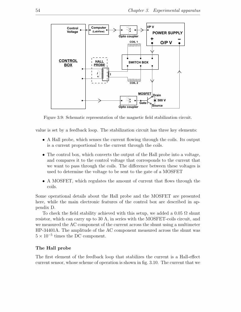
54 Chapter 3. Experimental apparatus
POWER SUPPLY
SWITCH BOX
COIL 1
COIL 2
500 V
O/P V
I/P V
Opto coupler
Computer
Opto coupler
GateSource
DrainMOSFET
HALLPROBE
ControlVoltage
Ii
CONTROLBOX
(LabView)
Figure 3.9: Schematic representation of the magnetic field stabilization circuit.
value is set by a feedback loop. The stabilization circuit has three key elements:
• A Hall probe, which senses the current flowing through the coils. Its outputis a current proportional to the current through the coils.
• The control box, which converts the output of the Hall probe into a voltage,and compares it to the control voltage that corresponds to the current thatwe want to pass through the coils. The difference between these voltages isused to determine the voltage to be sent to the gate of a MOSFET
• A MOSFET, which regulates the amount of current that flows through thecoils.
Some operational details about the Hall probe and the MOSFET are presentedhere, while the main electronic features of the control box are described in ap-pendix D.
To check the field stability achieved with this setup, we added a 0.05 Ω shuntresistor, which can carry up to 30 A, in series with the MOSFET-coils circuit, andwe measured the AC component of the current across the shunt using a multimeterHP-34401A. The amplitude of the AC component measured across the shunt was5 × 10−5 times the DC component.
The Hall probe
The first element of the feedback loop that stabilizes the current is a Hall-effectcurrent sensor, whose scheme of operation is shown in fig. 3.10. The current that we

3.4. Magnetic fields 55
want to stabilize flows in the direction of the thick arrow (Iprimary). This generatesa magnetic field that is trapped in a ferromagnetic core making a loop aroundthe current. This magnetic field crosses the semiconductor piece (shaded). Asmall current generator within the sensor generates a current Ic, that flows acrossthe semiconductor piece in a direction orthogonal to the magnetic field. In suchcircumstances an electric field arises in the direction orthogonal to both currentIc and magnetic field: this is called the Hall effect. The electric field leads to apotential difference that can be used to control a feedback circuit A to apply acurrent Isecondary on a secondary coil (N turns wound around the ferromagneticcore). For an appropriate value of Isecondary, the magnetic field generated by thissecondary coil cancels the field generated by the primary current. Now, whenthe magnetic field is cancelled inside the ferromagnetic core, the current in theprimary coil is N times bigger than the current in the secondary coil (the outputof the current sensor), whose value can be obtained by passing it through a knownresistor Rsense. The voltage Vsense across this resistor is strictly related to thecurrent that we want to measure, and can be used as the input of the feedbackcircuit that stabilizes the primary current to the desired value.
N turns ofsecondary coilaround themagnetic core
Isecondary
Rsense
IcIprimary
+_
A
Vsense~ I /NprimaryRsense
Figure 3.10: Scheme of a Hall-effect current sensor.
Our sensor is made by Honeywell (model CSNJ481). This can take up to600 A as an input current, and its secondary coil has 2000 turns, so that theoutput current is limited to 300 mA. We pass about 16.2 A through the coils toproduce 1000 G, so we wound the wire 20 times around the hole of the sensor toexploit more of the dynamic range of the Hall sensor and to have a better signalat low current.

56 Chapter 3. Experimental apparatus
The MOSFET
The MOSFET (Farnell, N TO-264) is used as a variable resistor, whose value isregulated by the gate voltage. It can take up to 38 A as a drain current, anddissipates 520 W at room temperature. In practice, the output voltage of themain power supply is set to be higher than it needs to be to ensure there is alwaysenough voltage available to push the required current through the circuit. Duringthe evaporation, when high currents are passed through the coils for up to a minute,the heating in the coils causes their resistance to rise and so the supplied voltagemust continually increase even if the current is to remain constant; obviously, fortoo high an output voltage, the excess power dissipated in the MOSFET overheatsit. To protect it against overheating it is mounted on a water cooled brass block.
As a further protection feature for the MOSFET, a Zener diode (500 V break-down voltage) is inserted between source and drain, so that when the current inthe coils is rapidly switched off, any induced e.m.f. between source and drainthat exceeds the MOSFET’s breakdown value of 600 V will not push current backthrough the MOSFET itself, but through the Zener diode.
Unfortunately, accidental overheating of the coils on one occasion caused theinsulating coating of the coils to melt (thankfully only on a single point), connectingthe coils to the optical table that is connected to ground. Instead of winding a newset of coils with all the replacement work that this would have required, we decidedto make the melted point the only ground connection in the circuit, and apply afloating voltage to the MOSFET. This was done using an opto-coupling circuit(built using the CHIP IL-300 by Vishay) to duplicate the gate voltage comingfrom the stabilization box (that had the same ground connection as the computersignal) into another identical voltage actually applied to the gate of the MOSFET,but without the same ground reference.
3.5 Pyramid MOT
The pyramid MOT is used as a source of pre-cooled atoms with which to feed thescience MOT. This preliminary stage is needed because to produce the BEC we usea magnetic trap, which has to be placed in a chamber where the level of vacuumis such that a MOT cannot be loaded by the vapour at room temperature. Thechoice of a pyramid MOT comes from wanting a cheap, simple, and reliable tool.The original design of its configuration is due to K.I. Lee et al. [81], but it was inOxford that it was first modified to make it a continuous source of slow atoms withboth caesium [82] and rubidium, adding a small hole at the vertex of the pyramid.Details of the function of such a tool can be found in the two references above.
It consists of a set of four mirrors in the shape of an inverted pyramid. There aretwo square mirrors placed at 90o next to each other, plus two prisms to completethe pyramid. The final result mounted in the vacuum chamber is shown in fig. 3.11.

3.5. Pyramid MOT 57
A hole of 1 × 2 mm2 was left at the vertex to allow the cooled atoms to travel tothe science cell. The side of the base of the pyramid is 6 cm long. The BK7 glasssubstrate for the mirrors was coated in our physics department. The coating isa broad-band dielectric coating that has similar characteristics for both s- and p-polarized light, and hence does not affect the polarization of the light.
Figure 3.11: The pyramid in which about 2 ·108 atoms are captured in a MOT. The sideof the base of the pyramid is 6 cm long.
The pyramid MOT is operated by a single beam travelling along the axis ofthe pyramid towards its base. This beam contains light for both cooling (59 mW)and repumping (3.5 mW) the atoms. The beam is magnified using a telescope toincrease its transverse diameter from 2.8 mm to 43 mm, so that it covers a largeportion of the base area of the pyramid ensuring a bigger capture region for theMOT.
As mentioned at the beginning of this section, this is a very simple and effectiveway to load the science MOT, and the various stages of optimization are now wellestablished procedures in our group. What is important is that they have all beenoptimized once also the other MOT was operative, to maximize the second MOT’sloading rate and its steady state value. The magnetic field gradient is 10 G/cm atthe centre of the trapping region. The cooling light is detuned 15 MHz on the redof the |F = 2〉 → |F ′ = 3〉 transition. The polarization of the beam is circular, andthe reflections on the mirrors of the pyramid make it so that in all points of thetrapping region the photons counter propagating in each direction have oppositepolarization (σ+/σ−).
The flux of atoms to the second chamber is strongly dependent on how well thezero of the magnetic field is aligned with the vertex of the pyramid, and on the

58 Chapter 3. Experimental apparatus
direction of the laser beam that, at the centre, acts as a push beam. The formerfeature is ensured firstly by centring the quadrupole field and the laser beam on theaxis of the pyramid, and then finely positioning it using the shim coils to slightlymove the zero of the magnetic field. The latter is controlled by a pair of mirrorswhich steer the direction of the laser beam, and a CCD camera that monitors thefluorescence of the pyramid MOT: when this is well aligned, the pyramid MOTis not visible on the CCD camera. The pyramid MOT reaches its full loading inabout 4 s.
3.6 Science MOT
The beam of slow 87Rb atoms produced with the pyramid travels for about 30 cm,and then is collected and trapped in a second MOT. This second MOT, or scienceMOT, (denoted MOT2 throughout this thesis) is a standard six-beam MOT.
The three pairs of counter-propagating beams are formed from the light comingout of the optical fibre. About 30 mW of power, including about 1.5 mW of therepumping radiation, comes out of the fibre and is split into six beams. Two ofthese beams counter propagate along the vertical direction through the centre ofthe glass cell. The other four form two counter-propagating orthogonal pairs inthe horizontal plane.
The quartz cell is attached to the vacuum chamber through a quartz-metaladaptor. The long side of the cell (7 cm) is the one in the direction of the incomingatomic beam from the pyramid, and its section is 2 × 2 cm2.
The laser beams have a diameter of about 20 mm, and a nearly perfect Gaussianprofile thanks to the mode filtering provided by the fibre. A half-wave plate isplaced just before each polarizing beam-splitter cube, to allow regulation of thepower-splitting ratio at each step. Each pair must be balanced in power, and thethree pairs have similar total power. Finally a quarter-wave plate for each of the sixbeams makes their polarization circular just before they enter the cell. The helicityof the polarization is chosen according to the schemes presented in chapter 2, andit is such that each counter-propagating pair has one beam polarized σ+, and theother polarized σ−.
A first rough alignment of the MOT beams is done by looking at the superpo-sition of the counter-propagating beams on white paper with an infrared viewer.Once this alignment is good enough for a tiny MOT to be observed, the alignmentof the beams, as well as the orientation of the quarter-wave plates, is improvedmaximizing the fluorescence of the MOT collected by a photodiode.
The main objective is to collect the largest number of atoms in the secondMOT, therefore maximizing this parameter (N) was the criterion used to choosethe values of the magnetic field gradient and the detuning of the laser beams.The current flowing through the dispenser was also determined by looking at thenumber of atoms in the second MOT. After an initial linear growth it would reach a

3.7. Imaging system 59
steady state value, and the turning point (I = 3 A) was chosen as initial dispensercurrent. It had to be increased little by little during the following months toensure constant quantity of rubidium in the pyramid chamber. Figure 3.12 showsthe measurements taken during the optimization process, and which lead to thechoice of δ = −2π × 14 MHz and ∇B = 14 G/cm as best operational parameters.
Figure 3.12: Optimization of the science MOT parameters. The scan of the field gradienthas been done keeping the detuning of the light at δ = −2π × 14 MHz, and the scan of
the detuning was performed keeping the axial field gradient at ∇B = 14 G/cm.
The choice of the current flowing through the shim coils was made by lookingat the temperature of the molasses. After this optimization process, we can loadup to 2× 10⁸ atoms in the second MOT in about 120 s. The lifetime of the atomswas measured by recording the decay of the fluorescence signal at different timesafter blocking the pyramid beam. An exponential fit of the data yields a 1/elifetime τ = 102 ± 7 s, as reported in fig. 3.13. The initial quick decrease in thefluorescence is probably due to light assisted inelastic collisions between two atomsin the MOT, one in the ground level and one in the excited level, that dominatethe losses at large numbers being proportional to N2. The time constant of theremaining decay is mainly determined by collisions between the trapped atoms andthe background vapour, which is proportional to the number N of trapped atoms.For these reasons the first data-point is not included in the fit.
3.7 Imaging system
This section describes how we take quantitative images of the atomic clouds. Adescription of the analysis performed on the images to extract physical informationabout the clouds is given in appendix B.
We used the well-established absorption imaging technique to observe our con-

60 Chapter 3. Experimental apparatus
Figure 3.13: Lifetime of the science MOT.
densates. A circularly polarized1 laser beam resonant with a closed atomic transi-tion is directed onto the atomic cloud (see fig. 3.14). Radiation gets absorbed bythe atoms so that a shadow of the cloud is cast on the CCD. The absorption profiledepends on the density and the shape of the atomic cloud. The absorption of theradiation, as it crosses the atoms in the y direction (under conditions specifiedbelow) is described by Lambert’s law [83]:
I=I0 · e−ky (3.5)
where k = nσ is the absorption coefficient, given by the density of the cloud timesthe absorption cross section, that can be written, in a regime of low saturation, as:
σ(δ)=σ0
1 + (2δΓ
)2(3.6)
where σ0 = 3λ2/2π, that in our case is ∼ 3 · 10−8 cm2, is the cross section for reso-nant absorption, and Γ is the natural line width of the transition involved. A tableof numbers relevant to the optical properties of 87Rb is reported in appendix A.The conditions under which equation 3.5 applies are:
1. The light must be monochromatic, that is to say the linewidth of the laser(during the probe pulse) must be much smaller than Γ.
1This is to maximize the absorption, when probing in the presence of a polarizing magneticfield.

3.7. Imaging system 61
2. The amplitude of the electric field should vary very slowly on distances ofthe order of a wavelength.
3. The radiation can be approximated with a plane wave.
The first condition is guaranteed by the locking of our lasers. The second one re-quires the size of the cloud that we image, and over which the intensity decays, tobe large compared to the probing wavelength. This is satisfied because a conden-sate has a diameter of the order of a few microns. The last condition arises fromthe consideration of whether the cloud acts as a lens to focus the light: in a regimeof low saturation, the Kramers-Kronig relations between refractive index and ab-sorbtion give a phase shift ∆φ ' (δ/2Γ) ln(I0/It), where I0 and It are the incidentand transmitted light respectively. For a red frequency detuning of the radiation,the medium becomes equivalent to a lens of focal length f = 2πl2/(∆φ λ), wherel is the size of the cloud along the direction of propagation of the light beam [84].Therefore, for the last condition to be satisfied, it is required that δ ' 0 (resonantprobe beam).
Our probe beam (of measured waist w0 = 3 mm) is resonant with the F = 2 →F ′ = 3 transition, and its intensity (0.9 mW/cm2) is about 30% of the saturationintensity. The probe pulse lasts for about 0.2 ms, to prevent saturation whenimaging a condensate. During the probe pulse the cloud falls about 30 microns;this effect limits the accuracy of our measurements of the size of the clouds. Wehave calculated that this effect increases the size of the condensate measured after15 ms of time of flight to be 20% bigger than if it were not falling. This affects thedetermination of the size, but not the number of atoms calculated from the picture,and since we do not use the size of the cloud to deduce any relevant physical result,we decided that it is not important to correct for this.
The blurring could be reduced by a faster probing pulse, but that would requiremore laser power on the camera to have the same signal. This extra power is neededon the camera to use most of the dynamic range of its chip, but would lead tomore saturation of the transition. The solution to this could be either to get a newcamera with a higher sensitivity, so that a shorter pulse of the same intensity couldmake use of the whole dynamic range of the CCD, or reduce the magnification sothat the the intensity hitting the camera is higher. Currently the magnificationenlarges the image of the cloud, and hence the whole probe beam by a factor2.59, reducing the intensity hitting the CCD by a factor 6.7. This magnification,however, gives images of the condensates that spread over a reasonable number ofpixels, even when imaged in trap without time-of-flight expansion. The side lengthof one pixel is 9 µm, hence the resolution of the imaging system is 9/2.59=3.47 µm.

62 Chapter 3. Experimental apparatus
3.7.1 Absorption pictures
The absorption imaging technique is a destructive one, i.e. the pulse of resonantlight destroys the condensate. To remove the background light from the image ofthe cloud we must take three pictures. The first records all the light that has notbeen absorbed by the atoms (IA). A second (bright) picture is taken in exactlythe same conditions as the first one, but without atoms, therefore it records thewhole intensity of the light (IB). A third (dark) picture is taken without firingthe probe, to record the background light (ID). A computer program subtractsthe last picture from the first two, and then takes the ratio of the two resultingframes. This ratio, T (x, z) = IA−ID
IB−ID, represents the transparency of the medium.
Its reciprocal is the opacity, and the logarithm of the opacity is, by definition, theoptical density of the medium. Therefore, the optical density D(x, z) is obtainedfrom the transparency T (x, z), using the relationship [2]:
D(x, z)=− ln(T (x, z)). (3.7)
The data are recorded as an array containing the optical density for each pixel.These data are used to extract physical information on the cloud such as density,number, and size (as discussed in appendix B).
3.7.2 CCD camera
To acquire the images we use a Spectra Source CCD camera (Teleris 2 ) with aKodak CCD array of 768 × 512 square pixels each with a side length of 9 µm.The overall size of the chip is 6.91 × 4.6 mm. It has a saturation capacity of8.5 × 104 electrons/pixel, and a specified quantum efficiency of about 40 % at780 nm. The very simple software that controls the acquisition of the framesthrough the computer (and clears the CCD array before acquiring each frame)allows acquisitions every 2 s. This means that the shortest time between eachpicture is about 2 s, thus the probe beam intensity must be very stable for about5 s. The quality of the background cancelation in our images shows that this isnot a problem with our apparatus.
The following simple calculation supports the choice of the intensity. Each pixelmust deliver less than 8.5×10⁴ e−, otherwise it will be saturated. If we aim for halfof this value (4× 10⁴ e−), with a quantum efficiency of 40 %, we require about 105
photons. The surface of each pixel is 8.1 × 10⁻⁷ cm2, therefore the energy neededon the chip per cm2 is u = hc
λ
Nphotons
S1pxl≈ 3 × 10⁻⁹ J/cm2. With a pulse that lasts
0.2 ms, the intensity needed to shine this energy on the CCD is I = 1.5 mW/cm2,and taking into account the magnification of the beam after it passes the cell, theintensity on the atoms must be I = 10 mW/cm2. Therefore, with the intensityI = 0.9 mW/cm2 specified earlier, we use about one tenth of the dynamic rangeof the CCD, and we are already almost saturating the transition. This is not theideal situation, but it did not significantly affect the quality of the data.

3.8. Computer control 63
3.7.3 Magnification and calibration
A schematic of the imaging system designed to produce a magnification of 2.5 isshown in fig. 3.14. The telescope consists of a pair of achromatic doublets of focallengths 40 mm and 100 mm respectively, spaced by a distance equal to the sumof the two focal lengths. The probe beam, collimated by the first lens after thefibre, is again collimated after the telescope, and the rays are normally incidentonto the chip of the CCD. In order to reduce the aberrations, the distance betweenthe atomic cloud and the telescope, and between the telescope and the surface ofthe CCD is as shown in fig. 3.14. The polarization is made circular by a polarizingbeam splitter cube followed by a quarter-wave plate before the cell.
f1 f1
f1=40
f2f2
f2=100
l/4
CC
D
Figure 3.14: Schematic representation of the imaging system.
Focussing was achieved by finely adjusting the position of the first lens. Thepixel size was calibrated by taking pictures of condensates for different time-of-flight, and fitting the free fall with a parabola (see fig. 3.15). The measured mag-nification factor was 2.59 ± 0.01.
3.8 Computer control
The LabView program (by National Instruments) has been used to achieve pre-cise control over several analogue devices and accurate time synchronization ofdigital and analogue devices on the experiment. The control program regulatesthe voltages sent to the VCOs which in turn control the frequency of the AOMs,the state of the mechanical shutters, and provide the control voltage to the powersupply of the magnetic field and of the stabilization box. Once the science MOTis fully loaded, we use this program to start a sequence that triggers and regulatesall the analogue and digital devices that are needed to load the magnetic trap,perform the evaporation to obtain the BEC, load the BEC into the optical traps,control the magnetic field required to produce the Feshbach resonance and duringthe ramps to create the molecules. Finally it also sets the imaging parameters andtriggers the probe pulses for the acquisition of the images.
The computer reaches all the electronic devices controlled by the program viatwo 12 bit PCI cards (National Instruments: PCI-6713, and PCI-MIO-16E-4).

64 Chapter 3. Experimental apparatus
Figure 3.15: Calibration of the imaging system magnification with time of flight images.
The first has 8 analogue outputs, and 8 digital outputs, while the second has 2analogue outputs and 16 analogue inputs, 5 digital outputs and 3 digital inputs.They both have 2 gated counters which are used for triggering the optical pumpingpulses, and flashes of lattice light with TTL signals. This did not provide sufficientdigital outputs, so an analogue to digital converter was designed, by the CentralElectronics workshop of our physics department, to generate 8 digital outputs fromone analogue output of the PCI-6713.

Chapter 4
Obtaining BEC
This chapter describes the experimental protocol that we used to produce a BEC of87Rb atoms in the |F = 1,mF = −1〉 state. Since it is a very standard procedure,I shall limit the content of this chapter to what is essential background for thisthesis, and to the issues relevant to our experiments.
The first section deals with the loading of the magnetic trap, in particularmode matching, i.e. the preparation of the cloud in a way that it maintains thephase-space density upon loading into the magnetic trap. The second sectiondescribes the evaporation protocol and its optimization in order to maximize thenumber of atoms in the final condensate. Initial measurements performed with thecondensates are briefly described in section 4.3.
4.1 Loading the TOP trap
As we have already discussed in the previous chapters, the densities and tempera-tures that can be achieved in a magneto-optical trap are not sufficient to reach thequantum degeneracy. To attain this, we need to employ evaporative cooling in atrap with no intrinsic cooling limits. This can be achieved by using a far-detunedoptical trap or a magnetic one. We make use of a TOP trap, which is the magnetictrap described in chapter 2.
The maximum energy of the atoms that can be trapped in the magnetic trapis limited by the potential depth µB0
4derived in section 2.3.1. As we want to trap
the biggest possible number of atoms in the initial trap, we will start with themaximum value of B0 achievable with our setup, which is 44 G. This fixes the trapdepth to about 370 µK (atoms in the |F = 1,mF = −1〉 state have a magneticmoment that gives µ/h = 0.7 MHz/G). This depth is well above the temperaturethat can be achieved by the molasses cooling phase, thus the pre-cooled atoms donot escape if they are in the correct magnetic state.
65

66 Chapter 4. Obtaining BEC
4.1.1 Mode matching
The initial trap, besides requiring a depth higher than the energy of the atoms,must have a profile that matches that of the cloud. For a harmonic trap potentialV = αr2, which has to host a cloud of mean energy 〈E〉 = 3
2kBT , we need the
size of the cloud in the i-direction to be σi ∼√
kBT/2α. Given the size andtemperature of the molasses, this relationship fixes the curvature of the harmonicpotential. For our experiment, we measured the temperature of the molasses to beabout 30 µK, and its radius 0.9 mm; hence α ≈ 2.5 × 10⁻²²J/m2. For the case of87Rb in a harmonic trap, this leads to a frequency in the radial direction of about60 rad/s. Equation 2.12 in chapter 2 provides the relationship between the trapfrequency and the magnetic fields generating the TOP potential. We have alreadystated the necessity of using the highest rotating bias field possible: B0=44 G;hence to obtain ωr = 60 rad/s, requires a magnetic field gradient b′ ' 100 G/cm(from eq. 2.12).
If the trap parameters are not those that give good matching, the kinetic energyand the potential energy are not balanced after loading, thus inducing a breathingmode (shape oscillations) to the cloud. Also oscillations of the center of mass ofthe cloud (sloshing), due to an offset between the position of the molasses andthat of the center of the quadrupole field, cause initial losses if the cloud reachesthe locus of B = 0. These oscillations were observed experimentally and we foundthat the breathing mode was negligible. The frequency of the sloshing oscillationsof the cloud has been used to obtain a calibration of the effective trap frequencyas a function of the magnetic fields (their amplitude was limited to about 270 µm,which is one order of magnitude smaller than the initial radius of the circle ofdeath).
To appreciate how much a mismatching affects the phase space density, we canlook at the diagram in fig. 4.1, which shows the phase space density (in units ofits initial value just before loading the trap) versus the trap frequency (in units ofthe value for an ideal matching). The function plotted is [85]:
ρ
ρ0
=8(ω/ω0)
3/2
(1 + ω/ω0)3, (4.1)
The diagram shows that having a trap of frequency higher than its ideal value isless harmful than under-matching. There is a range of about ±20% of the optimumtrap frequency, where the phase space density is not reduced appreciably. We loadthe atoms into a trap whose frequencies are within this range.
To maximize the phase space density of the cloud that is transferred into theTOP trap, we used a three stage transfer protocol (implemented in the LabViewprogram), to control the quantities relevant to the mode matching described above.In the first stage molasses cooling reduces the temperature of the atoms to about30 µK. In the the second stage we optically pump the atoms from the F = 2 level

4.1. Loading the TOP trap 67
0 0.2 0.4 0.6 0.8 1 1.2 1.4 1.6 1.8 20
0.2
0.4
0.6
0.8
1
ω [ω0]
ρ [
ρ 0]
Figure 4.1: Phase space density (in units of its initial value just before loading the trap)versus the trap frequency (in units of the value for an ideal matching).
in the MOT, to the |F = 1,mF = −1〉 state for magnetic trapping. The thirdstage is switching on the field to an appropriate initial trap strength.
The phase space density depends on the size of the cloud, as well as its tem-perature, therefore a compression of the MOT is sometimes performed just beforethe beginning of the optical molasses. In the compressed MOT, the gradient of thequadrupole field and frequency detuning δ of the laser are both increased. How-ever, we did not perform any compression of the MOT before the molasses cooling,because it was not found to be useful in our experimental measurements. Althoughthe phase space density is reduced by both the expansion of the cloud during themolasses phase and by the heating inferred by the optical pumping pulses, due tothe molasses cooling and to the short duration of the optical pumping, it remainedclose to the top of the curve of fig. 4.1.
4.1.2 Optical molasses
To change from a MOT to optical molasses the magnetic field is ramped downto zero in 2 ms, whilst at the same time increasing the frequency detuning of thelight. The cooling is thus provided by the sub-Doppler mechanisms described insection 2.1, giving a final temperature inversely proportional to δ, as given byeq. 2.3. The ramp is followed by further 4 ms of cooling at the final parameters.

68 Chapter 4. Obtaining BEC
In order to choose the final detuning for the molasses phase we plotted the phasespace density of the initial TOP trap against different values of this parameter,and this plot is shown in fig. 4.2. We decided to use -35 MHz since greater redfrequency detuning did not increase the phase space density significatively withinthe error bar, but gave fewer atoms. For the point at -50 MHz the number ofatoms was about half that for all the previous points.
Figure 4.2: Phase space density of the cloud loaded into the TOP trap just after themolasses phase as a function of the final detuning for the molasses.
For these measurements we left atoms in the F = 2 level without performingany optical pumping, thus loosing the fraction of atoms in magnetic sub-levels withmF ≤ 0. The number of atoms here is about 1 order of magnitude lower than thenumber of atoms actually transferred in the magnetic trap when we optically pumpthem into the |F = 1,mF = −1〉 state. Also the phase space density measuredhere is one order of magnitude lower than that of the |F = 1,mF = −1〉 atomsloaded in the initial trap.
The temperature reached with the molasses cooling was measured to be about30 µK by a time of flight technique, i.e. looking at the size of the cloud as a functionof time in free expansion.
4.1.3 Optical pumping
Different optical pumping strategies are possible to transfer the atoms into thestate |F = 1,mF = −1〉. We could have just switched off the repumping light atthe end of the molasses stage, but this only puts 1/3 of the atoms into the right mF

4.1. Loading the TOP trap 69
state. Optical pumping with σ-polarized light tuned on the |F = 1〉 → |F ′ = 1〉transition would give higher efficiency, but would have required an extra AOMon the optical bench to obtain the appropriate frequency. A simpler option is touse σ-polarized light tuned on the |F = 2〉 → |F ′ = 2〉 transition and switch therepumping light off. This does not need an extra AOM, and can also be usedto obtain a BEC in the level F = 2. To this end we only needed to switch thepolarization of the optical pumping beam from σ− to σ+, and have some repumperlight ON at the same time. We decided to use this second option for our opticalpumping. The selectivity of the transfer is obtained thanks to the σ-polarized lightand to the presence of a small (3.5 G) magnetic field that provides the atoms witha quantization axis.
To determine how many pulses to use (and which duty cycle) for an optimumtransfer, we experimentally scanned one parameter at a time (number of pulsesand duration), and recorded the number of atoms transferred in the magnetic trap.This process led to the choice of 15 pulses, each lasting 40 µs, of light detuned by5 MHz below (red) the centre of the |F = 2〉 → |F ′ = 2〉 transition. The magneticfield is provided by the TOP field, which rotates at 7 kHz, hence the pulses needto be synchronized in such a way that the direction of the magnetic field is parallelto the laser beam at the middle of the 40 µs pulse. About 0.9 mW of laser lightare sent to the atoms using the same optical fibre used for the imaging, thereforealso this beam has a 1/e diameter of 6.5 mm, and a peak intensity of about5.4 mW/cm2.
The whole optical pumping process lasts about 2.1 ms (since each of the 15pulses is synchronized with the rotation of the TOP field (7 kHz), which has atime period of 0.143 ms). There is a rise in temperature of the order of a fewrecoil energies, where 87Rb has Tr=360 nK (since λ=780 nm), meaning an overallincrease of about 1 µK. This is negligible compared to the 30 µK of the molasses.
Our optical pumping scheme transferred 70% of the atoms into the |F =1,mF = −1〉 state. That this transfer efficiency is entirely due to the opticalpumping pulses can be seen from the following considerations. As our probe beamuses light resonant with the |F = 2〉 → |F ′ = 3〉 transition, we need to transferthe atoms back to |F = 2〉 before the imaging. This is done by sending repump-ing light on the atoms for nearly 1 ms just before the probe pulse is fired. Thefact that no atoms are observed without this repumping stage before the imagingmeans that of the (30%) atoms not pumped in the state |F = 1,mF = −1〉, noneare left in the |F = 2〉; hence the remaining fraction is entirely pumped into the|F = 1,mF = 0, 1〉, and then lost during the magnetic trapping phase. Moreover, ifwe do not perform optical pumping before loading the magnetic trap, then probingwith or without repumping light does not change the number of atoms detected,which means that no atoms were in the |F = 1〉 state to start with.

70 Chapter 4. Obtaining BEC
4.1.4 Parameters of the initial trap
At the end of the optical pumping the atoms are ready to be trapped in themagnetic potential where their phase space density will be increased by means ofevaporative cooling up to and beyond the threshold of condensation.
To load the magnetic trap all the laser light is blocked and the magnetic fieldis quickly turned on. The atoms are now in a magnetic trap whose strength isdetermined by the combination of a quadrupole field, of gradient b′ = 95 G/cmalong the radial direction, with a rotating bias field of magnitude B0 = 44 G.These were chosen by looking at the temperature of the cloud loaded into themagnetic trap, and trying to minimize it. The harmonic potential generated bythese values of b′ and B0 has a radial frequency ωr ' 60 rad/s that nearly matchesthe frequency for which the plot of fig. 4.1 has a maximum.
The lifetime of the atoms in the magnetic trap was measured to be about 85 s,and a plot of this measurement is shown in fig. 4.3. The initial ten seconds wereleft out of the fit because we are only interested in the losses due to collisions withthe background atoms, which are determined by the vacuum level and thereforeare always present, and not in the initial rapid loss.
Figure 4.3: Measurement of the lifetime of the atoms in the loading TOP trap.
From the plot in fig. 4.3 we can see that in the initial trap we can load about108 atoms. These have an initial phase space density of about 4× 10⁻⁸. The eightorders of magnitude needed to reach the threshold of condensation are gained withthe evaporative cooling, in the way described in the next section.

4.2. Evaporative path to BEC 71
4.2 Evaporative path to BEC
We use evaporative cooling to reduce further the temperature of the cloud downto the critical temperature Tc, whose expression was given in section 2.4. Since Tc
depends on the number of atoms in the trap, the more atoms are removed fromthe trap during the evaporation, the lower the temperature needs to go in order toreach the degeneracy, so this process should be performed as efficiently as possible.During the evaporation each atom that leaves the cloud must take away much moreenergy than the mean energy. The speed of this process is regulated by the rateat which elastic collisions redistribute energy (which depends on the temperatureand density of the cloud).
The three parameters: temperature, number density, and phase-space density,are connected between them by the relationship ρ = CnT−3/2. The proportionalityterm C contains only fundamental constants and the mass m the atom, and for87Rb its value is C = 6.5 × 10⁻³⁰ m3K3/2. For an effective evaporation we haveto act on both n and T in order to increase ρ. Our starting point, for the atomsloaded into the TOP trap, is n ' 6 × 109 cm−3 and T ' 10−4K, yielding a phasespace density ρ ' 4×10⁻⁸. The other important parameter of evaporative cooling,the elastic collision rate, is given, in terms of the density of the cloud, the crosssection and the mean velocity of the atoms, by the relationship [2]
Γc =√
2 · nvσ (4.2)
where√
2 · v is the relative mean velocity between two atoms (with v =√
8kBTπm
),
and σ = 8πa2 is the cross section for elastic scattering (a being the scatteringlength). For a harmonic trap, moreover, the mean density is related to the trapfrequency by the expression [86]:
n = Nω3 ·(
m
4πkBT
)3/2
. (4.3)
And combining these two equations we get:
Γc ∝ω3
T. (4.4)
The rate of elastic collisions in the initial trap (from eq. 4.2) is Γc ' 1 s−1. Insection 2.5 we have seen that effective evaporation requires a ratio between elasticand inelastic collisions of about 300. This ratio can be estimated by the productof the elastic collision rate times the lifetime of the TOP trap, and in our case itis Γcτ ≈ 80 (for the initial trap). The first step of the evaporation must thereforebe to increase this parameter. The lifetime of the trap is limited by the vacuum,hence the quantity on which we can really act during the evaporation is Γc.

72 Chapter 4. Obtaining BEC
4.2.1 Increasing the collision rate
To have a larger rate of elastic collisions in the trap we adiabatically compressthe cloud (by increasing the magnetic field gradient). By definition this preservesthe initial phase space density. This adiabatic compression in a harmonic trapincreases the collision rate proportionally to the square of the frequency of thetrap; ρ stays constant, so: ρ ∝ nT−3/2 ∝ r−3T−3/2 ∝ r−6ω−3, where the last stepis possible because the temperature in a harmonic trap is given by T ∝ ω2r2.Therefore constant ρ implies r ∝ ω−1/2, hence T ∝ ω, which combined with eq. 4.4proves that Γc ∝ ω2 as stated.
The condition for the compression to be adiabatic is: dωdt
¿ ω2 [2]. During thefirst 4 s of the evaporation we nearly double the collision rate by ramping the fieldgradient b′ form 95 G/cm to 125 G/cm (b′ indicates the gradient of B along theradial direction, which is half the value it has along the axial direction). At thisearly stage we still want to minimize the evaporation, as it would not increase thephase space density; therefore, in order to have the largest possible radius of thecircle of death, we keep the TOP field B0 at its maximum value of 44 G. Thisfirst adiabatic compression just increases the elastic collision rate, bringing theproduct Γcτ to about half the value needed for the runaway regime. This targetwill anyway quickly be reached during the next ramp, when the stiffness of thetrap is increased by reducing the amplitude of the rotating bias field and furtherincreasing the gradient.
4.2.2 Evaporation with the rotating potential
The evaporation proper is carried out by ramping down the rotating bias field.Experimentally we determine the speed of the ramp for which the gain in phasespace density is highest compared to the loss in number of atoms. As we reducethe value of B0, the frequency of the trap goes up according to eq. 2.12; thisfurther compresses the atoms, thus increasing the collision rate and speeding upthe thermalization of the cloud, which allows faster ramps.
We found that an optimum slope for the phase space density against the numberof atoms was reached when the ramp was split into two steps. During a first step themagnetic field gradient was slowly ramped up to its maximum value b′ = 175 G/cmin 22 s, whilst at the same time the trap depth was reduced by decreasing the valueof B0 from 44 G to 9 G. The second step keeps the field gradient constant whilstfurther reducing the value of B0, in 8 s, from 9 to 3.5 G. Table 4.1 summarizesthe achievements of the evaporation up to this stage. We can see that the collisionrate has brought the system in the runaway regime already before the end of the22 s ramp, and that, so far, the gain in phase space density has been of about 5orders of magnitude, against a loss of about 2 orders of magnitude in the numberof atoms. The trend ρ ∝ N−2.5 is comparable to what found in many similarexperiments.

4.2. Evaporative path to BEC 73
Time (s) b′ (G/cm) B0 (G) N Γc (s−1) T (µK) n (cm−3) ρ
4 125 44 5 · 107 2 120 1010 2 · 10−8
22 175 9 107 20 40 2 · 1011 2 · 10−5
8 175 3.5 2 · 106 100 8 2 · 1012 10−3
Table 4.1: Values of some parameters relevant to the evaporation, at the end of each stage.
The radius of the locus of B = 0 is about 0.5 mm at the end of the 22 s ramp,and at the end of the 8 s ramp is only 0.2 mm. A further reduction of B0 led tolarge losses. From this point on, therefore, we complete the evaporation with theradio-frequency cutting, keeping the frequency and depth of the trap constant attheir final values: ωz/2π = 170 Hz, and U = 30 µK.
4.2.3 Radio-frequency evaporation
The starting point of the RF ramp can be calculated by considering the following:at any point on the circle of death the value of magnetic field varies between 0and 2B0 during one cycle of the rotating field. At the centre of the trap the fieldis B0. The condition for magnetic resonance between two consecutive Zeemansub-levels is hν = gF µB|B| (where gF is 1/2 in our case), therefore the variationof the magnetic field between 2B0 and B0 corresponds to a frequency sweep fromν = µBB0/h = 4.9 MHz (B0 = 3.5 G) to a value ν = µBB0/2h = 2.45 MHz; wherethe latter is resonant for atoms in the centre, i.e. at the bottom of the trap.
The RF-evaporation is performed in two steps. The first RF-sweep starts fromabout 5.2 MHz (just outside the circle of death), which is chosen to prevent ‘acci-dental’ evaporation before the start of the ramp (caused by any leakage of radio-frequency when the amplitude of the RF-amplifier is set to zero). Then we rampit down to 3.9 MHz in 9 s, gaining one further order of magnitude in phase spacedensity whilst halving the number of atoms. A plot of the phase space densityagainst the number of atoms during the different phases of the evaporation pro-cess is shown in fig. 4.4. The final ramp takes 5 s to sweep down to the thresholdof condensation, around 3.1 MHz, or below for a more pure condensate (below2.9 MHz no thermal component can be discerned).
Fig. 4.5 shows the formation of the condensate during the late stages of the RF-evaporation. The three pictures were all taken after 14 ms of time of flight. Thefirst picture shows a very cold thermal cloud (N = 8 × 10⁵, T' 500 nK, ρ=0.5).In the second picture a condensed peak appears in the middle of the thermal cloud(N = 5 × 10⁵, T'300 nK, ρ=2.8), and the last one is a pure condensate (about2×105 atoms) with no visible thermal component.

74 Chapter 4. Obtaining BEC
Figure 4.4: Plot of phase space density vs atom number during the evaporation.
3.4 MHz 2.9 MHz3.1 MHz
Figure 4.5: 3D plot in false colours of the BEC formation during the late stages of theRF-evaporation. The frequency underneath each picture indicates the final point of the
RF-sweep.
4.3 Additional measurements with the BEC
This section records two measurements performed after obtaining BEC that pro-vided us with a more accurate calibration of the TOP field. It is actually a doublecalibration, using two different methods. The first one is based on probing thecloud (using absorption imaging) in the presence of the rotating TOP field syn-chronized with the probe pulse; we keep the magnitude of the field constant whilevarying the detuning δ of the probe. The ‘number of atoms’ detected are plottedas a function of the detuning of the probe beam, see fig. 4.6 (this is the ‘numberof atoms’ calculated assuming resonant absorption, which is used as a measure of

4.3. Additional measurements with the BEC 75
the absorption). The absorption has a maximum at the detuning δ0 for which theZeeman shift µBB makes the transition resonant. From the value of δ0 we can workout the magnitude of the magnetic field through the relationship B = hδ0/µB. Toobtain the value of the peak detuning we assume a Lorentzian line shape, andfitting our data with this function shows that the previous value, coming form atheoretical prediction based on the geometry of the coils, was wrong by a factor1.72. For this measurement we used a very cold thermal cloud (with only partialRF-evaporation).
Figure 4.6: Calibration of the TOP field by measuring the Zeeman shift induced on theatomic levels.
The second calibration is based on the RF-cut in the final magnetic trap. Aswe have discussed above, the value of the radio frequency during the evaporationranges between two values determined by the top and the bottom of the magnetictrap, and their energy depends on the value of B0 alone. This provides a methodto calibrate the magnetic field by looking at which frequency we start to evaporate.Fig. 4.7 shows a plot of the number of atoms against the final frequency of theRF-cut. As its final frequency starts to drop below the top of the trap the atomsstart to be evaporated and a knee is observed in the plot. The horizontal linesindicate the average (with error) of the first 7 points on the right, and the diagonalline comes from a linear fit of the remaining points. The position of the knee isdetermined as the intersection of the two trends. Also this calibration suggests thesame factor 1.72, therefore we decided to adopt it to re-calibrate the magnitude ofthe rotating field.

76 Chapter 4. Obtaining BEC
Figure 4.7: Calibration of the TOP field based on the condition for magnetic resonanceduring the RF-evaporation.
4.4 Summary
In this chapter I have presented the results of the experiments that led to theproduction of BEC of 87Rb atoms in the |F = 1,mF = −1〉 state by means ofevaporative cooling in the TOP trap. The criteria adopted to choose the parame-ters for the transfer of the MOT into the magnetic trap, and subsequently thoseused to perform evaporative cooling have been discussed. With these parameterswe are able to transfer into the magnetic trap up to 2 × 10⁸ atoms in the desiredatomic state, and after 48 s of evaporative cooling we can produce pure condensateswith about 2 × 10⁵ atoms.
As a preliminary measurement, partially evaporated thermal clouds were usedto obtain a more accurate calibration of the rotating field in the TOP trap. Thiswas done by using two independent methods, one relying on the Zeeman shift of theatomic energy levels, and the other based on the condition for magnetic resonanceduring the RF-evaporation.
Chapter 5
1-D Optical lattice
After achieving BEC we set up a standing wave to trap the condensates in a one-dimensional optical lattice with the objective of observing the Feshbach resonancesthat occur in the |F = 1,mF = +1〉 hyperfine state of 87Rb [34]. This state, as wehave already said in the previous chapters, cannot be trapped in a magnetic trap.
The interest in atom lattices and in their possible applications to quantumcomputation, led us to this choice. Later, specific requirements of the moleculeproduction mechanisms, such as the density of atoms, and the aim to preservecoherence throughout the sample, led us to set up also a crossed-beam opticaldipole trap, to which the next chapter is dedicated.
In this chapter I shall go through the setup of the standing wave, illustrating itsconstruction and design features. The procedure used to align the standing waveonto the atoms is described in section 5.2. The last three sections are dedicated tothe loading and characterization of the atoms in the lattice, such as lifetime, trapdepth, and trap frequencies.
5.1 The standing wave
To set up our one-dimensional optical lattice we used a single vertical beam oflaser light, focussed to a minimum waist of 60 µm, and retro-reflected to form astanding wave. The light source was a pair of semiconductor diode lasers SDL-5422 operating at 850 nm, set up in the standard master-slave configuration. Theoptics involved is shown in the schematic of fig. 5.1. Being far off-resonance fromany atomic transition, we do not need to lock the laser frequency to any particularvalue. However, to form a standing wave, the laser frequency must be stable,therefore we used an external cavity master laser which operates single mode.
To monitor the laser mode and the injection of the slave we send the lightfrom both lasers into an etalon cavity (Tec Optics, FSR=3GHz), with no need
77

78 Chapter 5. 1-D Optical lattice
To vertical beam
850nmmaster
850nmslave
Fabry-Perotetalon
Figure 5.1: Schematic of the laser setup for the standing wave.
for saturated absorption spectroscopy. The slave laser follows the mode comingfrom the master over a frequency that is typically a few free-spectral ranges of theetalon. Some light from the two laser sources is deflected using beam splitters, sothat the status of the light can be monitored in real time on an oscilloscope duringthe experiment.
In order to reduce further the feedback from the retro-reflected beam, the lightfrom the slave laser is then passed through a second optical isolator. Subsequently,an AOM used in single pass acts as a fast switch for the lattice light. When theAOM is on, the first diffracted order is injected into a single-mode polarization-maintaining optical fibre. When it is off there is no diffracted order, hence thereis no light coupled into the optical fibre. This fibre, like those transporting lightto the MOTs, besides acting as a mode cleaner making the beam profile Gaussian,also decouples the alignment of the laser part of the table from the science cellarea.
Of the initial power (60 mW) in front of the fibre, about one half is coupledthrough it and, due to losses in other components and reflections on the cell sur-faces, only about 25 mW are available for the standing wave. In order to align the850 nm light along the same path as the MOT2 beams, we use two dichroic mirrors(DM), see fig. 5.2. These have been fabricated here at the department of physics,with a specially designed multi-layer coating that reflects linearly-polarized lightat 850 nm, and transmits 780 nm light. In tests these mirrors reflected 98% ofthe 850 nm light when it was horizontally polarized, and over 99% when it wasvertically polarized.
With a total power of 25 mW available for the standing wave, we can calculatefrom eq. 2.32 that a beam focussed to a waist of 50 µm, and retro-reflected, willgive a lattice depth of 80 Er. We decided to aim for such a deep trap so thatthe apparatus was suitable also for number squeezing experiments [87]. To obtain

5.1. The standing wave 79
780nm HR850nm R=0.99
l/4
780nm HT852nm HR
Doubletf=75
780nm
Translation stage
780nm HT852nm HR
850nm HR
850nm HR
M1
780nm HR780nm HR850nm R=0.99
780nm HR850nm R=0.99
l/2
l/4
Doubletf=40
CellMOT2
Bridge
MOT2 optics level
Laser bench level19.6
cm
14.7
cm
Bridge level
Laser bench level
Vertical section
M2
M2
M3
M3
DM
DM
M4
44mm
A
CB
Figure 5.2: Schematic representation of the optics to set up the lattice. (A) The outputof the lattice beam fibre is on the upper bridge of the optical table. The position ofthe doublet lens determines the waist size and its longitudinal position. Mirror M1 isthe one used to optimize the alignment onto the atoms. (B) On the lower level of theoptical table, mirror M4 is on a translation stage to optimize the spatial overlap of theretro-beam with the down-going beam. (C) Vertical section of the optical table around
the cell.
such a beam waist, a doublet lens of focal length f = 40 mm was placed 44 mmafter the output of the optical fibre. The core of the optical fibre has a radius of4 µm and so the waist of the laser beam exiting the fibre is comparable. Measuringthe size of this beam at two different points after the lens, and using the laws forthe propagation of Gaussian beams, we deduced that a waist of about 55 ± 5 µm

80 Chapter 5. 1-D Optical lattice
(1/e2 half width) would form 78 cm after the lens. This was consistent with thebeam having an initial waist given by the core of the optical fibre, and the waistposition was consistent with what we could judge by ‘eye’ observing the beam withan infrared sensor card.
The beam’s path length was then designed so that the focus of the beam fellat the trap position within a Rayleigh range 2ZR (ZR=10.4 mm for our measuredwaist and a wavelength of 850 nm). After crossing the cell, the beam is deflectedby the second dichroic mirror, which deflects the 850 nm light out of the pathof the 780 nm light. The deflected beam is focussed by a second doublet lens offocal length f=75 mm, to a waist of 12 µm onto the retro-reflecting mirror M4,positioned to form the standing wave (this mirror will be referred to as the retromirror throughout this thesis).
Obtaining a reliable measurement of the effective size of the standing waveat the position of the atoms is not easy, but this is a critical parameter for ourexperiments, and so it is worthwhile to briefly note some details here. The waistof the standing wave depends on how well we can superimpose the waist of theretro-reflected beam to the waist of the down-going beam. An independent, indi-rect measurement of the size of the latter comes from the measured values of theoscillation frequencies in the crossed-beam dipole trap, reported in chapter 6. Inchapter 2, we have derived the expression for these frequencies in eq. 2.49, and wecan see from there that ωy depends only on w1, which is the waist of the down-goingbeam, and on the trap depth. Working out the waist size from the value measuredfor the trap frequency ωy/2π = 67 Hz, we obtain 63± 6 µm. This overlaps, withinthe experimental error, with the value deduced by Gaussian beam propagation;but the large one suggests a shallower potential. The measured potential depthof the lattice was in the range of 11-15 Er (see section 5.4), which correspondsto an even bigger beam size (120 µm), but this is completely out of the error ofthese two measurements, suggesting that the lower lattice depth measured is dueto other factors such as a larger effective waist of the standing wave caused bythe retro-reflected beam having the waist in a slightly different z position, and/orpropagating in a slightly tilted direction.
5.2 Alignment procedure
A first rough alignment of the lattice beam onto the MOT was performed bycoupling light at 780 nm into the optical fibre used for the standing wave. Theprocedure was based on loading the second MOT and then, when it was fullyloaded, flipping a mirror to send 780 nm light through the optical fibre. Theflipping mirror was placed in the path of light going to the pyramid trap; thereforeduring this stage the second MOT was not being loaded anymore by the atomicbeam from the pyramid MOT. However, the nearly 80 s lifetime of the second MOTwas long enough to steer the direction of the down-going beam (acting on mirror

5.3. Loading of the atoms into the lattice and lifetime 81
M1) until it destroyed the MOT. Attenuating further and further the 780 nmbeam, we were able to see it acting as a push beam at the centre of the MOT(being this much bigger than the waist of the lattice beam). The procedure wasrepeated with a more compressed MOT (b′ = 20 G/cm) so that, since the 780 nmlight forms a waist very close in size and position to that formed by the 850 nmlight, we could set the direction of the beam accurately enough to observe someatoms being trapped into the standing wave at 850 nm. Small adjustments on theretro mirror enhanced this preliminary trapping effect. The angle and position ofthe retro mirror were optimized on the power of the light retro-reflected through thefibre. For the first alignment, iteration of this procedure was sometimes required.
At this point the alignment could be optimized, in the direction that can beseen by the CCD camera, by taking pictures of the BEC in trap, and of the atomsheld in the lattice. The lattice beam was moved until the atoms were held by thelattice in the same position where the BEC was formed. In the orthogonal direction(along the probe beam) this could not be done, so we optimized the alignment inthat direction by looking at the diffraction peaks of the BEC. This process will beaccounted for in a quantitative way in section 5.4, where the measurement of thestanding-wave potential depth is described.
5.3 Loading of the atoms into the lattice and life-
time
To reduce heating and losses, we loaded the atoms into the optical lattice adiabat-ically by slowly turning on the standing wave before switching off the quadrupolemagnetic field. The rotating bias field stays on to keep the atoms polarized (inzero field they would spin flip between the different Zeeman sub-levels). As usual,adiabatic means that the time taken to ramp the intensity of the lattice beam fromzero to 100% must be large compared to 1/νL, the inverse of the lattice frequency.The radial frequency of the standing wave is about 70 Hz, hence the ramping timemust be longer than 14 ms. We raise the intensity of the light linearly in a 50 msramp. Subsequently we ramp the gradient of the magnetic field b′ from 175 G/cmdown to zero in 100 ms (B0 = 3.5 G all the time).
When the alignment of the trap was improved, we observed a number of dif-ferent features of the periodic potential that helped us to check various aspectsof the system. A first experiment, when the lattice depth was about 1.5 Er, wasto generate a pulsed atom laser like the one observed at Yale in 1998 [16]. Theexperiment was performed by ramping the lattice power in 3 ms and keeping it onfor a variable time, counted from the subsequent switching off of the quadrupolefield, before taking a picture. As it is shown in fig. 5.3, pulses of atoms are emittedfrom the BEC with periodicity τ = 2π
ωB= 1.1 ms, where ωB = mgλ/2h is the Bloch
frequency at which the atoms oscillate in the lowest band, and are emitted at the

82 Chapter 5. 1-D Optical lattice
turning point of each oscillation.
Figure 5.3: Condensed atoms emitted by a lattice 1.5 Er deep, for three different holdingtimes. The axes are labeled in camera pixels, 1 pixel ' 3.5µm
Further improvement of the alignment made the trap depth sufficient to holdthe atoms in the standing wave alone, at which point we could measure the lifetimeof the lattice. We made this measurement for two different lattice depths. Thefirst time the lattice was about 8.5 Er deep, and the measured time for the numberto reduce of one half was τ1/2 = 1.7 ± 0.2 s. The second time the depth was11.7 Er and the measured decay time was τ1/2 = 0.9 ± 0.1 s. The data for thesemeasurements are shown in fig. 5.4.
For atoms loaded into the ground state of an optical trap from a BEC, 3-body collisions play a relevant role in the loss mechanism. It has been observedalso elsewhere, in agreement with our measurements, that longer lifetimes areachieved as the trap depth is reduced so that the atoms heated via collisions canescape the trap [88]. The dependence of the lifetime on the trap depth is notobvious, but it can qualitatively be understood in terms of density of the trapped

5.4. Measurement of the depth of the lattice 83
Figure 5.4: Decay of the number of atoms trapped in the lattice for two different trapdepths.
atoms. As the trap depth increases, the density (and therefore the rate of 3-body collisions) increases as well. If three body collisions are the main sourceof loss, then we have τ ∝ n−2, where n is the density of atoms in each latticesite, and the proportionality constant is the inverse of the three-body collision ratecoefficient. From the discussion in appendix C we can deduce that in each latticesite n ∝ a−1
h.o.zR−22D ∝ U , thus τ ∝ U−2. This is in good agreement with the two
measurements given above, i.e. (1.7/0.9) × (8.5/11.7)2 ' 1.. Therefore we shouldexpect for the lifetime of the atoms in a trap with depth U = 14 Er, as that usedfor most of the experiments described in chapters 7 and 8, lifetimes of the order of0.66 s. This time is still long compared to the duration of any experiment performedwith the atoms in the lattice. If we use this value of the lifetime for a 14 Er deeplattice, and the value of the mean square density 〈n2〉 = 2×10⁻²⁹ cm−6 as obtainedfrom equation C.7 of appendix C, the three-body collision rate comes out to be0.8 × 10−29 cm6/s, in good agreement with the value measured in chapter 7.
5.4 Measurement of the depth of the lattice
In order to compare the atom loss measured during the molecule formation exper-iments, we need to know the depth of the potential in which the atoms were held.This section explains how we experimentally measured the depth of the opticallattice by looking at the diffraction of the BEC released from a standing-wave po-tential. The theory involved in this technique has been described in section 2.6.1.
The size of a BEC is small compared to the Rayleigh range of the focussedlaser beam forming the trap, therefore we assume equal depth for all the wellspopulated. Moreover, the axial extent of the BEC is 6 µm, so we populate about30 lattice sites, which are half wavelength apart from each other (i.e. 425 nm), and

84 Chapter 5. 1-D Optical lattice
we can treat the majority of the wells as being in an infinite array. Therefore oursystem meets the requirements needed to use the theory in chapter 2, where weconsidered the case of sudden loading of the trap and subsequent evolution of thepopulated trap levels for a time τ . During this time the amplitude of the planewave components oscillates as shown in fig. 2.5.
Figure 5.5: Percentage of the population of the different diffraction orders as a functionof the time spent in the lattice.
Experimentally, we complete the evaporation in the magnetic trap, turn offsuddenly the magnetic potential, and immediately fire a pulse of lattice light ofduration τ . The different diffracted orders are allowed to separate thanks to theacquired different momenta 2mhk, where m = 0,±1,±2, ... indicates the order ofthe diffracted cloud. After a time t = 15 ms of expansion in free flight, the ordersare separated enough to measure the number of atoms in each of them. The zerothorder will have fallen as much as the BEC would have, and the other orders areseparated by ∆z = 2h
Mλt ' 160 µm. In fig. 5.5 the percentage of atoms measured
in each order is plotted against the duration of the lattice pulse. The positionof the minima and maxima of each order and their relative amplitude give thedepth of the lattice by comparison with the theoretical plot. To this end, the plotreported in chapter 2 (fig. 2.5) was made for a trap depth U0 = 11.3 Er, whichbest reproduce the experimental trend.

5.5. Measurement of the radial trap frequencies 85
5.5 Measurement of the radial trap frequencies
To the purpose of estimating the eccentricity of the profile of the lattice beam, wemeasured the frequency of radial oscillations of the atoms in the trap. To do sowe parametrically excited the trapped atoms by modulating the amplitude of thefrequency driving the AOM before the optical fibre. This results in modulationof the beam intensity (in our case 25% of its maximum value). The average trapdepth during this measurement was about 8 Er, and the experiment was performedon a very cold thermal cloud of about 2 × 10⁵ atoms.
Plotting the size of the cloud in the radial direction against the modulationfrequency we found two peaks, indeed showing that the beam profile was elliptical.The plot of the measurement is reported in fig. 5.6, where the two peaks arelocalized around 92 and 100 Hz, indicating two trap frequencies: ωr1 = 2π×46 Hz,and ωr2 = 2π × 50 Hz. The relationship between frequency and trap waist in thelattice is given in equation 2.39, and it shows a dependence ωr ∝ 1/w2
0, thus alsothe waist difference between the two axes is only of 4%, making the beam profileelliptical with eccentricity e = 0.28. This could be due to a slight misalignmentbetween down-going beam and retro beam.
Figure 5.6: Parametric excitation of a cloud of cold atoms trapped in the standing wave.As a measurement of the disturbance generated on the atoms, the radial size of the cloud,along the direction visible by the camera, is plotted against the modulation frequency.
The images are taken after 15 ms of time of flight.

86 Chapter 5. 1-D Optical lattice
This measurement of the radial frequencies can be used to obtain the effectiveaverage waist of the standing wave from the eq. 2.39, yielding w0 = 71 µm. Thisis slightly larger than the waist obtained for the down-going beam alone from theparametric oscillations in the crossed-beam dipole trap, which suggests that thedown-going beam and the retro-reflected beam cross at a slight angle.
5.6 Summary
In this chapter I have described how the 1D lattice has been set up and alignedonto the atoms. The choice of the loading parameters has been discussed, andwe have seen how the trap depth affects the lifetime of the lattice. The lifetimewas measured to be 1 s, and the maximum trap depth 10-15 Er (depending on thealignment), for a total power of the lattice beam of 25 mW. Finally, the radial trapfrequencies were also measured by parametric excitation of the trapped atoms.

Chapter 6
Crossed-beam dipole trap
The second type of optical trap set up for this experiment is a crossed-beam dipoletrap. The reason for doing this has been discussed at the beginning of section 2.6.2,where also the theory relevant to some features of this trap has been introduced.This second trap gave us the chance of trapping the condensates in a single trappingregion (unlike the standing wave). This chapter reports on the work done to setup (section 6.1), align (section 6.2), and characterize our crossed-beam dipole trap(sections 6.3 and 6.4).
6.1 The horizontal beam
This section describes the main features of the trap, in which two 850 nm laserbeams are focussed to a waist of about 60 µm, and cross each other orthogonallynear the centre of the magnetic trap. Of these two beams, one propagates alongthe vertical direction; it is the one used for the lattice, but without retro-reflection.The other beam propagates on the horizontal plane, and its setup is described here.
The main components of the laser system, shown in figure 6.1, are: a free-running laser diode, an AOM (which acts as a switch), and a polarization main-taining optical fibre. When the AOM is on, the first diffracted order goes into theoptical fibre, which brings it from the laser area of the table to the science cell area(onto the MOT2 optics level; see fig. 5.2). No frequency stabilization is needed forthis beam, because the light is so far detuned that the optical dipole force doesnot require a linewidth narrower than a free-running laser can provide.
Up to 65 mW of laser power is transmitted through the fibre and focussedto a waist of about 60 µm. Due to space constraints around the cell, it was onlypossible to make this beam cross the cell along the same axis as the imaging system(which is described in section 3.7). We did not want to alter the existing imagingsystem, and therefore we had to produce that waist using the telescope already
87

88 Chapter 6. Crossed-beam dipole trap
To horizontalbeam
850nmDiode Laser
Shutter AOM
Anamorphicprisms
Figure 6.1: Schematic of the laser setup for the horizontal beam.
present on that path, and used to magnify the images of the atoms. This is a1:2.5 magnifying telescope made of two doublets with focal lengths f=40 mm and100 mm, and placed at a distance that equals the sum of the two focal lengths.In order to have a 50 µm waist at the trap position, we need to have a 125 µm(= 50 × 2.5) waist at one focal length distance from the f=100 mm lens of theimaging magnifying telescope (see fig. 6.2). To achieve this, a doublet lens L1 offocal length f=30 mm was placed 30 mm after the fibre to have a collimated beam,and then a telescope (consisting of lenses L2 and L3, separated by 250 mm) wasinserted into the path to give the 125 µm waist, at the required distance from theimaging telescope.
Figure 6.2: Schematic of the set up used to align the horizontal beam onto the atoms.
The beam at 850 nm is deflected along the imaging direction using a dichroicmirror similar to that used to superimpose the standing wave with the MOT light,as described in section 5.1. The waist of the horizontal beam was found to belarger than the 50 µm in the original design. It is approximately 60 µm, as we

6.2. Alignment procedure 89
shall derive from the measurements reported in section 6.4.
6.2 Alignment procedure
As we can see from fig. 6.2, there are three lenses before the imaging telescope: L1is a doublet with f=30 mm, L2 has f=200 mm, and L3 has f=40 mm. MirrorM2, just before lens L3, is close to a focus of the beam, and therefore it is used forthe fine tuning of the transverse position of the waist on the atoms.
As with the standing wave, the alignment is performed in two main steps,repeated cyclically if needed. First we use weak light at 780 nm to align thehorizontal beam in such a way that it hits the centre of a compressed MOT (withb′ = 30 G/cm), as already described in section 5.2. Then, using 850 nm light, weact on the differential screws mounted behind mirror M2 for the fine tuning, whilemeasuring the shape, size, and temperature of the atoms loaded into the crosseddipole trap. A sufficiently well aligned trap gives round cold clouds after releaseand time of flight.
To double check that the waist of the beam was, also longitudinally, at theposition of the magnetic trap, we let a very weak beam (indeed, just the leakagelight from the AOM switched off) through the whole path, and then sent it ontothe chip of a CCD camera. The camera had been previously focussed on a verytightly compressed MOT, so that, by moving lens L2, the focus of the horizontalbeam was positioned on the magnetic trap within the diameter of a compressedMOT, i.e. a few mm. The pixel resolution of the monitor used for this processsuggested a beam size of about 40 µm. Even if the waist were this small, thebeam Rayleigh range would still be about 5 mm, which ensures that if the beamis focussed within a Rayleigh range, the beam size on the atoms would be at mostabout 60 µm.
6.3 Loading parameters and lifetime of the trap
For a good mode-matching we want the oscillation frequencies of the optical trapto be similar to those of the final magnetic trap, i.e. : ωr = 2π × 60 rad/s, andωz = 2π×170 rad/s. Equations 2.48-2.50 express the frequencies of the optical trapas a function of the trap depth and the beams waist; for a beam of waist 60 µm,the frequency is ∼ 100 Hz, when the power is 50 mW. We managed to obtain adiffraction efficiency of about 80% from the AOM, and by careful alignment wemanaged to couple 70% of the power into the optical fibre. Thus, from 125 mWbefore the AOM, with the laser running at the maximum recommended current, weget typically 66 mW out of the optical fibre. Reflections on the cell surface causea further 5% loss of power, to leave just above 60 mW at the atoms (therefore

90 Chapter 6. Crossed-beam dipole trap
we must push the laser very close to its maximum current, which can shorten itslifetime).
The adiabatic loading of the atoms into the trap was performed on the sametimescale used for the lattice. For trapping frequencies of the order of 100 Hz weneed ramping times slower than 10 ms. We find that ramping up the intensity ofthe light in 100 ms generated good dipole traps. The final powers were between90% and 100% of the maximum power for the horizontal beam, and between 50%and 100% for the vertical beam. The rotating bias field of the TOP trap wasmaintained at B0 = 3.5 G whilst the gradient was ramped down to zero in 50 ms.
For the maximum light intensity in both beams we measured the lifetime ofthe atoms in the trap. The procedure was again to make a BEC, then turn on theoptical trap in 100 ms, ramp down the magnetic field, and hold the atoms in theoptical potential for a variable time t. Fitting the decay of the number of atomsas a function of the time t spent in the trap, as shown in fig. 6.3, yields a lifetimeτ = 2.9 s. A longer lifetime than those reported for the lattice is obtained because,as explained in section 5.3, the crossed-beam potential has a lower depth than thestanding wave.
Figure 6.3: Lifetime of the atoms in crossed-beam dipole trap.
6.4 Measurement of the trap frequencies
This section describes the measurement of the trap oscillation frequencies carriedout to obtain information on the waists of the two beams. It was also used in

6.4. Measurement of the trap frequencies 91
deriving the depth of the trap; in doing this it is important to take into accountthe effect of gravity on the shape of the optical potential created by the crossed-beam, as described at the end of the section.
The trap oscillations frequencies were measured using parametric excitation ofthe cloud made by modulating the intensity of the beams (again this is achievedby modulating the AOM frequency, which, as an effect, modulates the injectioninto the fibre). Plotting the phase space density as a function of the modulationfrequency, we observed three values for which the excitation was obviously affectingthe phase space density of the cloud. One of these plots is reported in fig. 6.4, whichrepresents the excitation of the frequency along the horizontal beam by modulatingthe intensity of the vertical beam.
Figure 6.4: Parametric excitation of the oscillation frequencies of the atoms in thecrossed-beam dipole trap.
As we are only interested in estimating the position of the centre, we used aparabolic fit, which localizes the position of the minimum around 113.5 Hz, yield-ing a trap frequency ωy/2π = 57 ± 5 Hz. Similar measurements were performedin the other directions. Only two thirds of the power available to the verticalbeam was used, while the horizontal beam was at 90% of its maximum inten-sity. The extrapolated frequencies, at full power, for all the three directions are:(ωx, ωy, ωz) = 2π × (116 ± 10, 67 ± 6, 82 ± 7) rad/s. These are not in the exactrelationship derived in eq. 2.48, but they fall within the error bar. We also see thatthese frequencies are not very different from the frequency of the final TOP trap.
Using equations 2.49 and 2.50, with U0i given by eq. 2.47, we can derive thewaist of the two beams. Putting these equations together, we obtain a dependence
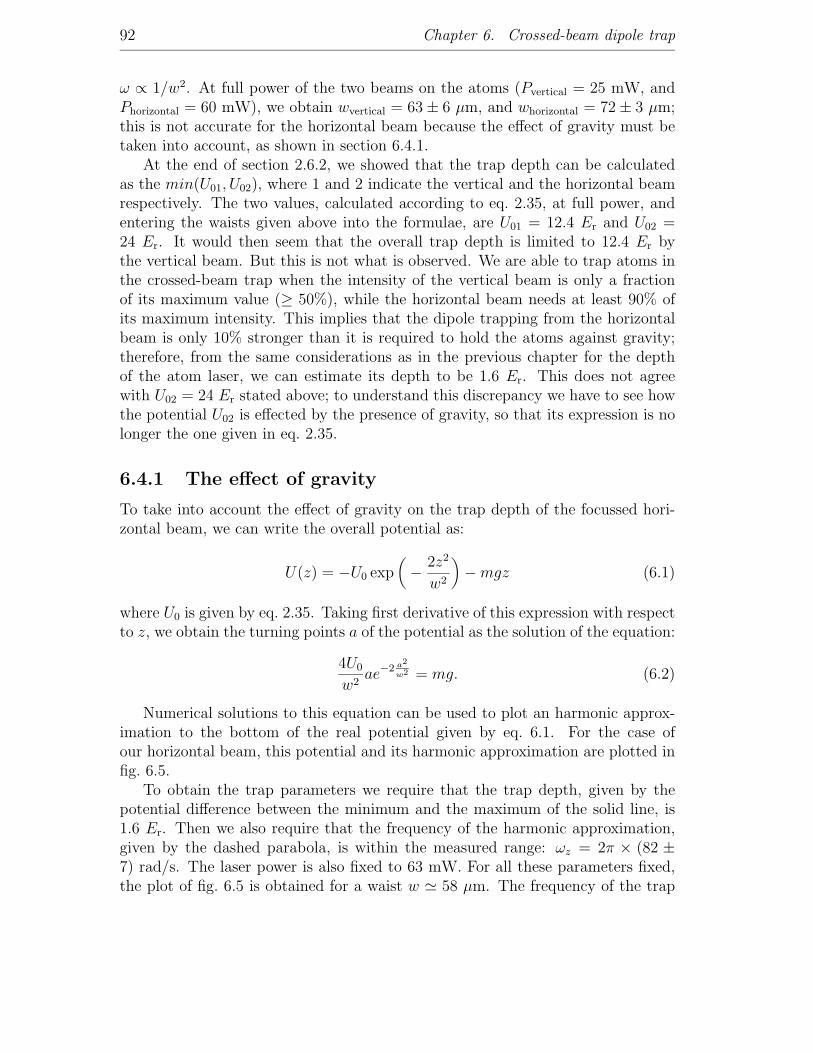
92 Chapter 6. Crossed-beam dipole trap
ω ∝ 1/w2. At full power of the two beams on the atoms (Pvertical = 25 mW, andPhorizontal = 60 mW), we obtain wvertical = 63 ± 6 µm, and whorizontal = 72 ± 3 µm;this is not accurate for the horizontal beam because the effect of gravity must betaken into account, as shown in section 6.4.1.
At the end of section 2.6.2, we showed that the trap depth can be calculatedas the min(U01, U02), where 1 and 2 indicate the vertical and the horizontal beamrespectively. The two values, calculated according to eq. 2.35, at full power, andentering the waists given above into the formulae, are U01 = 12.4 Er and U02 =24 Er. It would then seem that the overall trap depth is limited to 12.4 Er bythe vertical beam. But this is not what is observed. We are able to trap atoms inthe crossed-beam trap when the intensity of the vertical beam is only a fractionof its maximum value (≥ 50%), while the horizontal beam needs at least 90% ofits maximum intensity. This implies that the dipole trapping from the horizontalbeam is only 10% stronger than it is required to hold the atoms against gravity;therefore, from the same considerations as in the previous chapter for the depthof the atom laser, we can estimate its depth to be 1.6 Er. This does not agreewith U02 = 24 Er stated above; to understand this discrepancy we have to see howthe potential U02 is effected by the presence of gravity, so that its expression is nolonger the one given in eq. 2.35.
6.4.1 The effect of gravity
To take into account the effect of gravity on the trap depth of the focussed hori-zontal beam, we can write the overall potential as:
U(z) = −U0 exp(
− 2z2
w2
)
− mgz (6.1)
where U0 is given by eq. 2.35. Taking first derivative of this expression with respectto z, we obtain the turning points a of the potential as the solution of the equation:
4U0
w2ae−2 a2
w2 = mg. (6.2)
Numerical solutions to this equation can be used to plot an harmonic approx-imation to the bottom of the real potential given by eq. 6.1. For the case ofour horizontal beam, this potential and its harmonic approximation are plotted infig. 6.5.
To obtain the trap parameters we require that the trap depth, given by thepotential difference between the minimum and the maximum of the solid line, is1.6 Er. Then we also require that the frequency of the harmonic approximation,given by the dashed parabola, is within the measured range: ωz = 2π × (82 ±7) rad/s. The laser power is also fixed to 63 mW. For all these parameters fixed,the plot of fig. 6.5 is obtained for a waist w ' 58 µm. The frequency of the trap

6.5. Summary 93
0 0.005 0.01 0.015 0.02 0.025 0.03 0.035 0.04 0.045
−0.2
0
0.2
0.4
0.6
0.8
1
1.2
1.4
1.6
1.8
z axis [mm]
Pot
entia
l [ E
r ]
Harmonic oscillator freq. = 2 π ⋅ 89 Hz
Figure 6.5: Plot of the potential of the horizontal beam as a function of z. The dashedline represents the harmonic approximation to the bottom of the potential.
is determined by the curvature of the dashed parabola: ωz = 2π× 89 rad/s, whichis just within the measured range. Besides, the centre of the trap is shifted downalong z, indicating a gravitational sag of about 20 µm. It is worth noticing that89 Hz is the value of ωz which fulfills the relationship of eq. 2.48, when ωx and ωy
have the measured values given earlier.
In fig. 6.6 the potential of eq. 6.1 is plotted again, but on a much more expandedscale, in order to show the full profile. For comparison, this time the dashed linereproduces the same potential in absence of gravity. We can see from this plotthat the effect of the term mgz on the potential is to reduce its depth U0 by tiltingthe Gaussian profile of the beam intensity. Therefore, in order to account for themeasured trap frequency, and for the apparent trap depth, the beam waist at theposition where the atoms are trapped must be about w ' 58 µm. This is veryclose to the value already indicated by the considerations of section 6.2.
6.5 Summary
This chapter has described how the crossed-beam optical dipole trap used in thisexperiment has been set up and aligned onto the atoms. We have also discussedthe loading parameters and how a lifetime for the trap, of about 3 s, has beenmeasured. The measurement of the trap frequencies has been presented, and it

94 Chapter 6. Crossed-beam dipole trap
−0.1 −0.08 −0.06 −0.04 −0.02 0 0.02 0.04 0.06 0.08 0.1
−20
0
20
40
60
80
100
z axis [mm]
Pot
entia
l [ E
r ]
Potential of a focussed beam plus gravity
Figure 6.6: Extended plot of the potential of the horizontal beam as a function of z. Thedashed line represents the optical potential without gravity.
has led to a discussion on the effect of gravity on the depth of the potential. Thisdiscussion has shown that the trap depth is dramatically reduced by gravity.

Chapter 7
Observing a Feshbach resonance
This chapter describes the experimental work performed to localize and character-ize the Feshbach resonance that occurs around 1007 G in the state |F = 1,mF = 1〉of 87Rb. I would like to stress, yet again, that this state cannot be trapped in themagnetic trap, therefore these experiments are performed keeping the atoms in theoptical traps described in chapters 5 and 6.
In order to look for the resonance, the first step is the transfer of the atomsfrom the state |F = 1,mF = −1〉, where they are when we make the condensate, tothe state |F = 1,mF = 1〉. This transfer is achieved with an RF sweep at low field,and is described in section 7.1. Then, section 7.2 will deal with the observation ofthe Feshbach resonance. Lastly, section 7.3 will report on the measured increasein the 3-body loss rate when approaching the resonance.
7.1 RF transfer
After loading the atoms in one of the two optical traps, and before performingthe actual transfer of atomic state, we must switch the direction of the currentflow in one of the two magnetic coils to generate a homogeneous field rather thana quadrupole field, as described in section 3.4.5 of chapter 3. The switching ofthe connections to the coils is carried out while the current is zero, and then it israised again, this time to generate a weak uniform field of 10 G. The reason fordoing the transfer at low field is that the Zeeman effect is linear, and the splittingbetween the levels mF = −1 and mF = 0, and the levels mF = 0 and mF = 1is the same. To estimate the efficiency of the transfer we put the atoms back inthe magnetic trap (after the RF sweep); the magnetic field gradient has differenteffects on the three different m-states, so that these appear as distinct clouds inthe t.o.f. images.
95

96 Chapter 7. Observing a Feshbach resonance
At a field of 10 G the Zeeman splitting between the sub-levels of the F = 1 levelin 87Rb, in frequency units, is given by µB
h= µBB
2h' 7 MHz. Therefore, in such a
magnetic field, atoms initially in the state mF = −1 will undergo transitions intothe other magnetic levels when in the presence of RF at 7 MHz.
In order to obtain a complete transfer from the initial state to the final desiredstate we use an adiabatic RF sweep. This allows us to follow the avoided crossingof the levels as we sweep down the frequency through the point where the RF-coupling is maximum (7 MHz), as illustrated in fig. 7.1. To determine how slowthe ramp must be to be adiabatic, we use the relationship τ = 2∆ν/Ω2
R [89], where∆ν is the frequency range of the sweep, and ΩR is the Rabi frequency (proportionalto the amplitude of the RF).
6 6.5 7 7.5 8 8.5 9 9.5 10−4
−2
0
2
4
RF [MHz]
Ene
rgy
[MH
z]
B=10G
6 6.5 7 7.5 8 8.5 9 9.5 100
0.2
0.4
0.6
0.8
1
RF [MHz]
Prob
abili
ty
mF=+1
mF=0
mF=−1
Figure 7.1: (Above) Zeeman energy levels in the presence of RF at 7 MHz (the zero isthe energy of mF = 0). (Below) The evolution of the population during the downward
frequency scan, when starting with all the atoms in the level with mF = −1
The strength of the RF field was estimated for the geometry of the coils and themaximum driving current; this very rough calculation suggested that τ must belonger than 0.4 ms. What we do in practice is to set the sweep time to be 20 ms andthen reduce the intensity of the RF signal to the lowest possible that still allows atransfer efficiency into the level mF = 1 of nearly 100%. The advantage of using alow power is that it makes the coupling region of the lower plot in fig. 7.1 narrower,

7.2. Localizing the resonance 97
thus the end of the ramp is in a region where the interaction is practically absent.After the transfer, the magnetic field was increased from 10 G towards the
position of the resonance at 1007 G. Although at the end of the ramp the amplitudeof the RF is turned to zero, we ramp the frequency from higher values to lowervalues, so that the system is insensitive to an accidental overlap of the end of thetransfer stage with the beginning of the magnetic field ramp.
The timings of the complete transfer sequence are as follows: after switchingto the Helmholtz configuration we ramp up the field to 10 G in 10 ms, wait for1 ms, and then apply the RF signal, ramping its frequency from 10 MHz downto 6 MHz in 20 ms. The asymmetry of the frequency range with respect to the7 MHz is an extra safety feature to make sure that all the population initiallyin the mF = −1 is transferred. At the end of this process the fraction of atomsremaining in other states is not measurable, and we see that more than 99% ofthe atoms are transferred into the level mF = 1 where the Feshbach resonance at1007 G occurs.
We use a Stanford Research System frequency generator (DS-345) to generatethe RF sweep, which is applied through a 10 turn coil of 2 cm internal diameterplaced about 6 cm away from the atoms. To increase the RF amplitude, the fre-quency generator is attached to a home-made RF-amplifier, built using a Motorola40 dB amplifier accepting maximum input 0 dBm. We found optimum transferefficiency when using the RF amplifier with an input power of -3 dBm, i.e. about37 dBm of output.
7.2 Localizing the resonance
Once the atoms are all in the desired state, we need to raise the magnetic field tothe value where the resonance had been predicted and observe the atom loss. Inpractice we have to localize the resonance position within our own calibration ofthe magnetic field.
The experimental procedure is schematically illustrated in fig. 7.2. The cloud issubjected to a homogenous magnetic field, Bf , for a fixed time and the reduction ofthe number of atoms by collisions was recorded. The enhanced scattering length,as the field gets closer to the resonance, causes greater losses. During the entireprocedure, which lasts 200 ms, the atoms are trapped in the standing wave. Themagnetic field is ramped up linearly in 50 ms from the initial value of 10 G (usedfor the transfer) to a few Gauss above or below the resonance, so that the rampspeed of 20 G/ms makes the cloud insensitive to the other narrow resonances foundat lower fields [34]. Then the field is ramped in 2 ms to the final value Bf close tothe expected position of the resonance. The magnetic field magnitude is then keptat the final value Bf for 100 ms, before ramping it down to zero, again in 50 ms.The optical trap at this point is turned off, and after 15 ms of time of flight theatoms are imaged using the usual technique.

98 Chapter 7. Observing a Feshbach resonance
50 ms 100 ms 50 ms
Bf
Appliedfield
0
IMAGE
time
Opticaltrap
15 mst.o.f.
Figure 7.2: Time scheme of the procedure used to localize the Feshbach resonance.
The procedure described above is then used to localize the resonance by lookingat the minimum of the plot of the number of atoms as a function of the finalmagnetic field of the ramp. Such a plot is shown in fig. 7.3.
Figure 7.3: Number of atoms left in the trap after being exposed to a homogeneousmagnetic field of magnitude Bf for 100 ms. The solid line is a Lorentzian fit used only
to determine the position of the peak of the loss curve.
The asymmetry of the number of atoms probed below and above the reso-nance is due to the 2 ms ramp crossing the resonance to reach the field above. ALorentzian fit of these data gives an estimate for the position of the centre of theloss curve as 1005.25 G. But, as explained in section 3.4.5, at around 1000 G ourcalibration of the magnetic field was accurate to about 3 G, therefore this must be

7.3. Measurement of the 3-body loss rate 99
the resonance that was predicted to occur at 1007.4 G. A similar loss curve centredat 1007.34 G was obtained in the work presented in [34] where the observation ofthis resonance was first reported. A few months later the same group reported acomplete characterization of this resonance [64] by obtaining a plot of the scat-tering length as a function of the magnetic field. The width ∆B was found to be0.2 G, and the value for the centre of the resonance B0 was found to be 1007.4 G,in good agreement with the theoretical predictions [34].
7.3 Measurement of the 3-body loss rate
To take into account the effect of the enhanced scattering length on the trappedatoms at the resonance position when looking for the formation of molecules, wehave to understand what sort of losses are induced on the cloud as we sweep throughthe resonance. To this end, two types of measurement have been performed.
The first of these two studies provides us with a measurement of the dependenceof the 3-body loss rate on the increased scattering length for magnetic fields closeto the resonance. The second study measures the atom loss as a function of themagnetic field ramp speed when swept upwards across the resonance. This isdescribed in the next chapter together with the loss curve due to a downwardramp where the molecules should be formed.
The rate equation for the 3-body losses (see eq. 2.52) can be integrated overthe time ∆t = 0.1 s during which the atoms are held at the field Bf (assumingthat the trap volume stays constant whilst the number decreases), to find that K3
is related to the losses observed by:
Kc3 =
[(
N0
Nf
)2
− 1]
2〈n20〉∆t
(7.1)
The initial mean square density in the trap is 〈n20〉, and N0 and Nf are the number
of atoms at the beginning and end of the time interval ∆t. The experiment wasperformed with condensed atoms, therefore the rate constant obtained is Kc
3, whichis the rate of 3-body collisions in the BEC (six times smaller than K3 for a thermalcloud). The presence of this factor 1/6 had already been experimentally shownin [65]. It arises from the third order correlation function for ideal bosons. Thiscan be understood in terms of an analogy with the intensity fluctuations presentin a beam of photons, where the same physics accounts for the short-time photonbunching in a thermal light beam demonstrated by the Hanbury-Brown-Twissexperiment. In a thermal cloud of bosonic atoms, it is 3! times more likely thatthree atoms will be found together than in a BEC of the same mean density.
To determine the initial number N0 we performed the process described aboveto obtain the loss dip (from where we get the values for Nf), but without the

100 Chapter 7. Observing a Feshbach resonance
pausing for 100 ms at the Bf , and without quite reaching the resonance position;in this way any losses that do not occur in the 100 ms wait period are excludedfrom consideration. The other parameter that we need is the initial mean squaredensity (〈n2
0〉) in the trap, which is obtained for the atoms loaded in the lattice asexplained in appendix C.
Applying eq. 7.1 to the data plotted in fig. 7.3, along with N0 = 3.2 × 10⁵ and〈n2
0〉 = 2 × 1029 cm−6, we obtain the values of Kc3 for different magnitude of the
magnetic field. These are plotted in fig. 7.4.
Figure 7.4: The dependence of the 3-body collision rate Kc3 on the magnitude of the
magnetic field in a 87Rb BEC.
The value for Kc3 away from the resonance is obtained using a Gaussian fit
with a floating background (this has the sole purpose of determining the positionof the centre and the asymptotic value of the wings). From the fit we obtainKc
3 = 9 ± 2 10−30 cm6/s far away from the resonance, which increases by nearly 2orders of magnitude as we get to the resonance centre. The position of the centreis also determined from the fit, and its value B0 = 1005.28 ± 0.03 G obviouslymatches the one determined from the atom loss curve of fig. 7.3. An estimateof the value of K3 is 6Kc
3. This gives 5 × 10⁻²⁹ cm6/s away from the resonanceand a peak value of 5 × 10⁻²⁷ cm6/s. The error bars in fig. 7.4 only account forthe statistic uncertainty of the measurements. The experiment was performed inan optical lattice (not in the crossed-beam trap), and the mean square density of〈n2
0〉 = 2×1029 cm−6 given above is an average of the mean square densities acrossthe 30 wells populated.
In fig. 7.5 the three-body loss rate obtained for 87Rb (K3 = 6Kc3) is compared

7.3. Measurement of the 3-body loss rate 101
with a theoretical curve that comes from a 3-body calculation (provided by T.Kohler, Oxford). In fig. 7.5 an offset was added to the magnetic field in order tohave the resonance at 1007.4 G and allow a direct comparison with the theory.
Figure 7.5: Comparison between the experimental values and the theoretical plot of thedependence of the 3-body collision rate K3 on the magnitude of the magnetic field in
87Rb.
Theory and experiment show a good agreement relative to previous comparisonsfound in the literature, as one can see, for example, in [90, 91]. The first of these twopapers compares experimental and theoretical three-body recombination constantsin a system without resonance enhancement, whilst the second is about fermions,and reports on p-wave resonance enhanced three-body recombination. Althoughthese results are not directly comparable to ours, they give an idea to what extentthree-body recombination processes can be predicted. Going back to our plot,we can see that the agreement improves going towards the resonance; this is dueto the fact that the 3-body collisions play a more significant role in the losses aswe get closer to the resonance. More details on the theoretical approach to thecalculation can be found in [92, 93].

102 Chapter 7. Observing a Feshbach resonance
7.4 Summary
This chapter has described how atoms in an optical trap are transferred from theatomic state |F = 1,mF = −1〉, in which they are in the TOP trap, into the state|F = 1,mF = 1〉 where a number of Feshbach resonances in 87Rb have been found.
The experimental procedure used to localize the Feshbach resonance at 1007 Gis explained, and a measurement of the 3-body collision rate is reported as afunction of the magnetic field close to the resonance. The measured values for K3
show reasonable agreement with the theory.

Chapter 8
Search for Molecules
This chapter deals with the experiments performed to investigate the formation ofultracold molecules exploiting the Feshbach resonance around 1007.4 G studied inthe previous chapter. To this end, sections from 8.1 to 8.3 discuss the choice of theramp speeds used when crossing the resonance both upwards and downwards, andsection 8.3 also shows the experimental study performed in order to understandthe role of density in the production mechanisms during the magnetic field ramps.Once the key points for the molecule production have been established, section 8.5presents the experimental protocols used to look for the molecules, while the de-tection methods employed are explained in section 8.4. Unfortunately none ofthe measurements performed by us showed conclusive evidence of the productionof ultracold molecules. The causes that we believe to be responsible for this arediscussed in section 8.6.
8.1 Introduction
From the theory of the molecular formation with the Feshbach resonance, discussedin the last section of chapter 2, we see that in order to form molecules we need tocross the resonance going from negative to positive scattering length. In our casethis means that we need to start with a magnetic field higher than the resonancevalue. Since we start at zero field, this means that we need to cross the resonanceas we sweep upward to reach the starting point. Our apparatus cannot detectmolecules directly, for example through photo-ionization. Thus the strategy wasto produce the molecules, separate them from the remaining atoms, and thenconvert the molecules back into atoms by reversing the field ramp before probingat zero field. This can be achieved by the ramps shown in fig. 8.1, explained indetail at the end of this section.
103

104 Chapter 8. Search for Molecules
Br
Appli
ed f
ield
0
IMAGE
time
Optical trap ON
Burstramp
Molecularramp
Dissociationramp
Separationtime
Figure 8.1: Schematic of the experiment. After ramping the magnetic field to 1000 G, aburst ramp (the name is justified later in this section) is used to go above the resonancevery quickly to reduce losses. Then the molecular ramp crosses the resonance at a certainspeed to form as many molecules as possible. These, during a separation time spent a fewGauss below the resonance need to be separated from the atoms using one of the methodsdescribed later in this chapter. Subsequently an upward ramp across the resonance isneeded to dissociate the molecules again into atoms for probing. Finally, the magnetic
field is switched off to be able to use the usual imaging technique for the atoms.
A diagram showing the energy levels of the channels involved as a function ofthe applied magnetic field is reproduced in fig. 8.2. The open channel correspondsto unbound atoms in the state labelled by |F = 1,mF = +1〉 at low fields. Theclosed channel corresponds to the bound molecular state which is coupled to the|F = 1,mF = +1〉|F = 1,mF = +1〉 channel by an s-wave Feshbach resonance at1007 G.
Figure 8.2: Diagram of the energy levels in the open and closed channels around theresonance as a function of the magnetic field.
In an upward sweep (see fig. 8.3 A), if atoms in the open channel adiabaticallyfollow the energy level across the region of the avoided level-crossings, they end up

8.1. Introduction 105
in excited trap levels, and possibly in untrapped levels. In both cases these atomswill not contribute to the molecule formation during the molecular ramp, as themolecular state can only be reached from the ground state (see fig. 8.3 B). To stayin the ground state we have to cross the resonance fairly quickly in order to jumpthe avoided crossing.
E
BBr
Closed Channel
Open Channel
Radial vibr.Levels
Second lattice band
Ground state
Burst ramp E
BBr
Resonance state(closed channel)
Open Channel
Molecular ramp(A) (B)
Figure 8.3: Diagram illustrating the effect on the atoms in the ground state of the openchannel (BEC) of: (A) the upwards (burst) ramp, and (B) the downwards (molecular)
ramp.
The basic steps for the production and detection of molecules can thus besummarized as follows:
1. Sweep the magnetic field up to a few Gauss above the resonance rampingthe field very quickly through the resonance itself. This is usually referred toas a burst ramp, because the loss during this ramp arises from the enhancedenergy of some atoms with respect to the energy of the condensate, and theseatoms escape from the optical trap. So the name is used in analogy to aneffect studied at JILA [94], where it was used to address the loss of atoms ina similar experiment with 85Rb.
2. Ramp back down across the resonance at the most favourable speed (to bedetermined experimentally) to produce molecules. This ramp will be referredto as the molecular ramp (see fig. 8.3 B).
3. Separate the associated molecules from the remaining atoms.
4. Ramp back up in order to dissociate the molecules back into atoms.
5. Ramp the magnetic field quickly down to zero and probe the atoms in theusual way.
Before looking at the specific production protocols adopted, let us examine theeffect of the burst and molecular ramps on the atoms.

106 Chapter 8. Search for Molecules
8.2 Burst ramps
The first study performed was the measurement of the loss of atoms during theburst ramps to determine the initial number of atoms remaining before the actualmolecular ramp.
The ramp used for this part of the experiment is shown schematically in thediagram of fig. 8.4. After ramping the magnetic field up to 2 G below the resonanceat a rate of about 20 G/ms, we pause for 5 ms to make sure that the current hasreached the asymptotic value (i.e. that the magnetic field does follow the signalfrom the computer). Then we increase the magnetic field by 4 G (to 2 G above theresonance) in time τramp, pause at this upper value of B for 3 ms before ramping themagnetic field down (crossing the resonance as fast as we can: about 100 G/ms)and then we finish by ramping back to zero field in a further 20 ms before detectingthe remaining atoms.
Figure 8.4: Schematic of the magnetic field ramp used in experiments to observe theeffect of the burst ramp.
Fig. 8.5 shows the measured relative atom loss: [Nc(ti) − Nc(tf )]/Nc(ti), as afunction of the inverse ramp speed during a linear ramp. For this set of data atypical number of atoms was Nc(ti) = 5×10⁴. The dotted line shows the expectedvalue for the atom loss of the ground state during the burst as calculated usingthe many body theory while the dash-dotted line shows the same parameter asobtained using the Landau-Zener result given in eq. 2.57, where δLZ is obtainedfrom eq. 2.58 (both courtesy of K. Goral). The solid line (half of the many bodyvalue) is printed only to guide the eye through the trend of the experimental points,and is not a fit to our data. To hold the atoms during the ramps we used a latticeof potential depth 11 Er. The measured loss is smaller than the theoretical curves.This is probably due to the fact that the formula gives the loss from the groundstate whether the atoms are expelled from the trap or are only promoted to anexcited trapped state which is still present in the absorption picture. Unfortunatelythere is no clear bimodal distribution that distinguishes them from the atoms inthe BEC, therefore we were not able to count them as lost. We only performed this

8.2. Burst ramps 107
measurement with the crossed-beam dipole trap at two ramp speeds: 0.05 ms/Gand 1 ms/G. Both traps exhibited comparable loss at these two speeds: about 15%for the fast burst ramp (0.05 ms/G), and about 40% at 1 ms/G.
Figure 8.5: The fraction of atoms lost during the burst ramp; (•) with a longitudinallymisaligned lattice, () with a better aligned lattice. The dotted line shows the expectedvalue using the many body theory while the dash-dotted line shows the Landau-Zenercalculation [Courtesy of K. Goral]. The solid line (half of the many body value) is printed
only to guide the eye, and is not a fit to the data.
The dip around 3 ms/G, seen in fig. 8.5 (solid circles), was consistently observedin the first batch of data taken at this lattice depth. But this effect disappearedafter having improved the overlap along the longitudinal axis of the waists of thedown-going and retro-reflected beams (open circles). This mismatch was partly thereason why initially we could not achieve standing waves deeper than 11 Er. Thedata shown as open circles were taken after improving the longitudinal alignment(but reducing the intensity to have again the same depth), and the feature wasnever observed again. We speculate that it may be due to the fact that when theretro beam forms its minimum waist in a different longitudinal position from thedown-going beam, the overall optical potential has a larger radial extent. Thissituation may let atoms which have been promoted to even more excited radialvibrational states of the potential remain trapped and be probed (see fig. 8.2). Forvery fast or very slow ramps the two alignment configurations lead to the sameobserved losses. In the case of very fast ramps this can be explained because morehighly excited states can be populated that are not kept by either trap. In the caseof a slow ramp it is mostly the low-lying radial vibrational states that are excited,which are probably safely trapped by both traps. Although the exact mechanism

108 Chapter 8. Search for Molecules
is not clear, the fact remains that the atoms detected include some which are notin the ground state, but, as said above, there is no clear bimodal distribution thatdistinguishes them from the atoms in the BEC.
To make molecules, the burst ramp is needed to reach magnetic fields abovethe resonance prior to molecule formation. For this we wanted the smallest losses,so we chose the fastest ramp speed of about 0.05 ms/G, giving losses only around15%. We also used an upward ramp to dissociate molecules back into atoms. Thisrequired slower ramp speeds of around 1 ms/G, where the loss is as high as 40%.This loss is not a problem because this ramp acts as a burst only on the atoms thatwere never converted into molecules and which we do not want to detect anyway.
8.3 Molecular ramps
The second study was performed with downward ramps, or molecular ramps, atdifferent speeds. The magnetic field was swept from above the Feshbach resonanceto below, as illustrated in fig. 8.6. After ramping the magnetic field magnitudein 50 ms to about 10 G below the resonance, we suddenly jump to a value some50 G above the resonance (at 0.05 ms/G) to make sure that the burst ramp haslittle effect on the initial number of atoms. Then we allow a settling time of 3 msat 5 G above the resonance before ramping down to 1 G above the resonance in0.5 ms. The molecular ramp linearly crosses the resonance, in variable times, toend 1 G below it. After a short waiting time at this final value of the magneticfield (typically 1 ms, and at this stage the optical trap had already been turnedoff), we ramp the field down to zero over 10 ms, and allow a further 4 ms of timeof flight before imaging. The total time of flight is counted from when the opticaltrap is switched off.
Figure 8.6: Schematic of the experiment to observe the effect of the molecular ramp.
The density of the cloud at the time of crossing the resonance depends on theparameter τfree fall, which indicates the time between the moment when the opticaltrap is switched off and the time when the magnetic field crosses the resonance

8.3. Molecular ramps 109
position; we can estimate the density at that stage from the expansion of thereleased condensate (as explained below). When the resonance is crossed whilethe atoms are still held in the trap, there is no free fall, and a negative number isused to indicate the amount of time the atoms and molecules formed have beentogether in the trap (see fig. 8.7). The number of atoms before the molecularramp was about 9 × 10⁴ for atoms held in a lattice, and 4 × 10⁴ for atoms in thecrossed-beam dipole trap.
The relative atom loss induced by the molecular ramp is plotted in fig. 8.7for different traps and free fall times. Denser atomic clouds show higher lossesdue to higher rates of molecule formation. For a lattice released 1 ms beforecrossing the resonance the dependence of the relative atom loss as a function ofthe ramp speed is also reported on the graph. Slower sweeps lead to more adiabatictransfer into molecules, and hence to higher atom loss. Two theoretical calculationsfor this case are also shown in fig. 8.7. The dotted line represents the Landau-Zener result (namely, the evaluation of eq. 2.57 with the Landau-Zener parametergiven by eq. 2.58 reported in chapter 2), while the solid line represents the resultof a many-body calculation (microscopic quantum dynamics approach) describedin [66]. These theoretical curves have been calculated by K. Goral (Oxford) fora mean density of 1013 cm−3 and agree reasonably well with the 1 ms expansionlattice curve, at least for slow ramp.
Figure 8.7: Measurement showing the percentage atom loss versus the inverse rampspeed during a molecular ramp; for an inverse ramp speed of 1 ms/G measurement atdifferent densities are shown. [X-dipole indicates the crossed-beam dipole trap]. Thedotted line is the Landau-Zener theoretical calculation for the lattice after 1 ms t.o.f.,
and the solid line is the many-body calculation (by K. Goral).

110 Chapter 8. Search for Molecules
For the BEC released from the crossed dipole trap, the density has been cal-culated using the expansion law given in [95]. For the experiments with atoms re-leased from the standing wave we estimate the density considering that the cloudhas very quick expansion in the tightly squeezed axial direction, while the ex-pansion in the radial direction can be neglected over 1 or 3 ms. In table 8.1 arereported the number densities obtained from this calculation for the different casesexamined experimentally.
τfree fall (ms) n/1012 cm−3 (Lattice) n/1012 cm−3 (X-dipole)
-1 150 501 13 303 8 -
Table 8.1: Densities of the atom cloud at the moment the magnetic field was crossing theresonance during the molecular ramp. Positive free fall times mean that the optical trap hadbeen switched off τfree fall ms before crossing the resonance, whilst a negative time means that
the optical trap was switched off τfree fall ms after having crossed the resonance.
Within the two channel approach used in [66] to describe the adiabatic asso-ciation of molecules by ramping linearly through the resonance, the losses in theatomic cloud are supposedly caused by the association of the atoms into molecules.Therefore we see that a slow ramp is best, and that the slower the ramp the betterthe molecule production. Bearing in mind the hypothesis that losses are due tomolecule formation, we can deduce from fig. 8.7 that, the denser is the cloud, themore efficient is the production of molecules. But there are some practical consid-erations to be made. The lifetime of these molecules is very short. As explainedin chapter 2, this arises because the most likely separation of the two associatingatoms is so small that the de-excitation of the molecules to lower bound states dueto 3-body collisions between free atoms and the coupled pairs is highly probable.This de-excitation becomes more probable in denser systems. These considera-tions, and the lack of a complete theory describing such loss mechanisms, meanthat a range of ramp speeds must be experimentally investigated in order to de-termine the optimum balance between the requirements of (a) reducing the lossesdue to de-excitation by increasing the ramp speed, and (b) increasing the efficiencyof the production of molecules by reducing the ramp speed.
The experience of a similar experiment [63] suggests that a ramp speed of1 ms/G to cross the resonance and go 2 G below it converts 10% of the atomsinto molecules. We found higher losses for the same ramp speed. As for the atomdensity, we explore all the possibilities, but the density reported in [63], for theatoms at the moment of crossing the resonance, has the same order of magnitudeas that of our atoms trapped in the crossed-beam dipole trap.

8.4. Separation methods 111
8.4 Separation methods
As already stated, we cannot detect molecules directly, but must dissociate themback into pairs of free atoms before imaging. The fraction of atoms associated intomolecules must be spatially separated before dissociation and imaging. At leasttwo methods are possible for distinguishing the molecules from the atoms. Oneexploits the difference in the magnetic moments of the atoms and molecules: theStern-Gerlach method adopted in [63]. The other relies on the diffraction of theatoms and molecules from a pulse of the standing-wave potential, which works ifthe molecules retain some of the coherence of the original condensate. These twomethods are described in detail here, while the complete experimental protocolsfor both, and the observations will be left to the next sections.
8.4.1 Diffraction
The idea behind this method is to flash the standing wave onto the atoms andmolecules to observe diffraction as shown in section 5.4. Provided the moleculesand the atoms are still coherent they should also spatially separate from each otherdue to their different masses (resulting in the diffracted momentum states of themolecules having half the velocity of the atoms) as described below.
The procedure itself is very simple. At the end of the molecular ramp we sitfor 1 or 2 ms at the final field (1 or 2 G below the resonance) and during this timethe standing wave is flashed on the mixture of atoms and molecules. Moleculeshave twice the mass of the atoms, hence the separation between the diffractedorders should be half the separation between the diffracted orders of the atoms.The central orders will always be superimposed, but the first diffracted order ofthe molecular cloud should sit in the gap between the zeroth and the first orderof the atoms. After the pulse we need to ramp up the magnetic field to dissociatethe molecules and then switch it off very quickly, and allow some further time offlight before detection.
The experiment is a very ambitious one, because it would separate spatiallythe atoms from the molecules only if the whole system remains coherent. It isalso very tricky from the point of view of the signal to noise ratio, as it aims todetect a small fraction of atoms coming from the dissociation of the molecules ineach diffracted order. Even assuming that all the molecules, for a specific pulselength, populate the first order, and that 7% of the initial atoms are convertedinto molecules, we would only have about 3000 atoms in each of the two diffractedorders of the molecular cloud (the number of the condensate atoms held in thecrossed dipole trap before the molecular ramp is about 4 × 10⁴). Moreover, aftera sufficiently long time of flight so that the atomic orders are separated enough toshow the presence of the molecular diffracted order, the optical density of such atiny number of atoms would be almost at our detection limit. The positive aspect

112 Chapter 8. Search for Molecules
of this experimental approach, however, is that the standing wave can be appliedvery quickly after the molecular production so that the atoms and molecules canbegin to separate immediately, thus reducing the number of de-excitation collisions.
8.4.2 Stern-Gerlach experiment
This method was successfully used in [63] to show evidence of the formation ofmolecules in a similar experiment, and whilst it does not give information on thedegree of coherence of the associated molecules, it has the advantage of creatingonly one molecular cloud (which increases the signal to noise ratio in the images)and allows the atoms and the molecules to be separated further apart than can beachieved with the other method during a typical experimental time-of-flight.
The technique relies on the different magnetic moment of molecules and atomsto separate them with a magnetic field gradient. Experimentally, at the end ofthe molecular ramp, the field sits at the final value for a variable time, typically2 ms, during which an inhomogeneous magnetic field with a gradient of 21 G/cmalong the vertical axis is applied to decelerate the gravitational fall of the moleculeswhilst it further accelerates the atoms in the direction of ~g. Just before rampingup again for the dissociation of the molecules, the Stern-Gerlach field (gradient)is turned off. In the meantime the molecules should have fallen only a smallamount, whilst the atoms have moved downwards a large amount. At this pointthe experiment can continue as usual, with dissociation ramp and imaging, and allthe atoms imaged in the upper cloud should have previously been molecules.
The value of the magnetic field gradient to levitate molecules for the Stern-Gerlach separation is obtained experimentally by looking at the gradient for whichthe molecules are supported against gravity, when in a field 2 G below the reso-nance. This is calculated from the requirement:
mg =dE
dz=
dE
dB
dB
dz(8.1)
where m is the mass of the molecule, dBdz
is the field gradient, and the slope dEdB
depends on the magnetic field as shown in fig. 2.9. For the resonance state, the slopedEdB
was measured in [63] as a function of B, and 2 G below the resonance it is about1.2 MHz/G. This requires the gradient of the levitating field to be about 35 G/cm.Unfortunately, we cannot reach that field with our Stern-Gerlach coil. For theatoms in the state |F,mF 〉 = |1, +1〉 the magnetic moment (obtained by taking thefirst derivative with respect to B of the Breit-Rabi formula given in equation 3.3)is about -1 MHz/G, leading to a required levitating gradient of 21 G/cm, andin the opposite direction as the one required to levitate the molecules. We canproduce 21 G/cm, and we applied this gradient in the direction that opposes thefree fall of the molecules (being only 3/5 of the required levitating field), whilstpushing down the atoms with an extra force. To prevent further collisions between

8.5. Experimental protocols 113
the atoms and the molecules we need to separate completely the two clouds assoon as possible. This is safely achieved by applying the field gradient for 2 ms, asshown by the following simple calculation. The size along z of the probed cloudafter 3 ms of time of flight is σz = 13 µm, therefore to separate the atomic cloudfrom the molecules, i.e. to achieve ∆z = 2σz, we need to apply the Stern-Gerlachfield for a time t such that the distance fallen by the molecules during that timeis at least ∆z shorter than the distance covered by the atoms. For the atoms wehave ∆zA = gt2, while for the molecules we have ∆zM = 1
5gt2, so the difference in
position will be ∆z = 45gt2. Therefore, the minimum time for which we have to
apply the field, in order to separate the two clouds by at least 2σz, is t = 1.3 ms.
8.5 Experimental protocols
The initial part of the protocol is identical to the one described in section 8.3, up tothe time when we get to 1 G above the resonance. Up to this stage the optical trapis always present. Next, the molecular ramp follows, in which the magnetic fieldis ramped linearly down to 2 G below the resonance, i.e. 1003.25 G, since in ourcalibration the resonance is centred at 1005.25 G (see section 7.2). Alternativelywe would ramp linearly to just above, at, or below the resonance and then jumpto 1003.25 G in 0.1 ms (see fig. 8.8).
Figure 8.8: Magnetic field ramps for associating and dissociating molecules.
This field was kept for 2 ms before starting the dissociation ramp with a shapesymmetric to the molecular ramp. During these 2 ms either of the two separationmethods described above were applied in order to spatially isolate the associatedmolecules. Next, the magnetic field is ramped down to zero for detection in about10 ms.

114 Chapter 8. Search for Molecules
Figure 8.9: Schematic of the experimental routine for the production of molecules.
In a first series of experiments aimed at observing the formation of molecules(see fig. 8.9), the optical trap was switched off at different times during the molec-ular ramp in order to vary the density of the atoms when crossing the resonance,as discussed in section 8.3. No molecules were seen to be converted back to atoms.
Performing the experiment in free fall has the advantage of giving a handle onthe density of the atoms at the moment of the association, but has the disadvantageof making us rush through all the sequence due to the long time required to turnoff the magnetic field.
Figure 8.10: Schematic of the experimental routine for the production of molecules inthe optical trap. To separate the atoms from the molecules, a Stern-Gerlach is applied
during the 2 ms stage before the molecules are converted back into atoms.
To eliminate the long time of flight problem, we tried experiments entirely inthe optical trap (see fig. 8.10). In this case we used the Stern-Gerlach field gradientto selectively get rid of the non-associated atoms from the trap during the 2 msstage before the dissociation ramp. No molecules were observed using a crossed-beam dipole trap. We also tried with the standing wave, but this time beforethe molecular ramp started we reduced the intensity of the optical trap beam toa value such that it was possible to expel atoms from it with the 21 G/cm fieldgradient. No signal was observed this way either. But this method was never very

8.6. Limitations of the experimental setup 115
reproducible because the amount of losses was very sensitive to the depth of thelattice.
We must therefore analyze the possible causes of the non-observation of themolecules. One possibility of course is that the molecules were never produced inthe first place, but this seems unlikely because the amount of 3-body loss duringthe molecular ramp, as we have seen, does not account for the observed loss, andtwo body inelastic collisions can be ruled out as they cannot lead to spin relaxationof the electronic ground state. Higher order losses at that density are even lesslikely. We assume then, as a starting point, that of the observed 45% atom lossduring the molecular ramp, only a fraction survives the collisional de-excitation,and comparison with similar experiments would suggest that this should be atleast 10% of the initial number. The question is then, where has the remaining10% gone?
One possible explanation is that the molecules were never converted back intoatoms, but this seems unlikely, because we have tried dissociation ramps for manydifferent speeds around those for which molecules had been successfully convertedinto atoms in another experiment.
A second possible explanation is that the dissociation energy was so high thatdue to the long time of flight the optical density of the small atomic cloud comingfrom the dissociated molecules was too small to emerge over the background noise.In order to avoid this we should take images after a shorter time of flight. Thismeans either probing at high field, or switching off the magnetic field more quickly.Unfortunately we are not able to do the latter due to the long decay time of ourmagnetic field. The causes of this long decay time must be looked for in thefeatures of our experimental apparatus discussed in the next section. While as faras the former option is concerned, it would have involved setting up a differentlaser system to realize a closed loop transition for the atomic level splitting around1000 G, and locking these lasers nearly 1 GHz away from their low-field resonance(which would have also required some expensive pieces of apparatus). This optionwas not pursued because, by the time we had got to this stage, the experiment hadalready been performed successfully at Max-Planck Institute for Quantum-Optics(MPQ) in Garching [63]. It did not seem that, with our apparatus, our methodwould have explored enough interesting new physics to justify the effort and theexpense required. We then decided to move on to a different experiment, for whichour apparatus is more suitable, as it is explained in the last chapter.
8.6 Limitations of the experimental setup
I should recall that the initial option we pursued to probe the molecules had beento separate them from the unconverted atoms, dissociate them back into atomsand then probe these atoms using the usual probing transition at zero field. Ourexperiment showed no evidence of these atom clouds coming from the converted

116 Chapter 8. Search for Molecules
molecules, but the overall time of flight after dissociation had been always at least15 ms. This long time was dominated by the 13 ms needed to make sure thatthe field was down to zero at the moment of taking the image. In the experimentperformed at MPQ the equivalent ramp takes only 2 ms. Our coils though, aremade of 400 turns, so that the effect of the inductance is large. We consideredcompletely opening the circuit which takes the current to zero within the responsetime of the control box (about 1 ms), however, a Hall probe detector placed atvarious locations along the vertical direction near the coils detected a residual fieldcaused by eddy currents which decayed with a time constant of about 10 ms. Thisresulted in an even longer time for the final field to fall to zero than by rampingthe current in the coils. We tried to reduce the eddy currents by dismantling thesupport for the coils and optics, and cutting slots in various places to preventclosed loops that could act as an electrical circuit. This did not help much becausethe radial component of the magnetic field created eddy currents that circulatealong vertical planes on the metallic mount supporting the coils.
A different design of the coils, with less turns and more current could haveallowed the field to be ramped down more quickly, and eddy currents could havebeen reduced with non metallic coil-supports. This again would have required alarge change to the apparatus, which did not seem justified after molecules hadalready been created at MPQ. The existing coils had only been designed to producea quadrupole field, and in that case the field at the centre is always zero so therewould never be problems with imaging after a short time of flight. Moreover thecurrent for our strongest TOP trap is about 10 A, which is two thirds of the currentneeded to generate 1000 G, and so also the eddy currents generated during thequadrupole field phase decay much more quickly, and no effect was ever observedon the atoms.
8.7 Summary
This section has described the experimental procedures used to exploit the Fesh-bach resonance at 1007 G in 87Rb to associate condensed atoms into molecules.The relative atom loss in ramping the field across the resonance has been mea-sured in both upwards ramps and downwards ramps. In these latter ramps theassociation is supposed to be the only possibility for losses in a two-body treatmentof the dynamics, but, although about 45% of the atoms were observed to be lostduring this molecular ramp, no signal was observed if the non-associated atomswere removed before dissociating the molecules again into atoms.

Chapter 9
Conclusions and outlook
This thesis has presented the construction, optimization, and operation of an ap-paratus capable of producing Bose-Einstein condensates of about half a million87Rb atoms in a TOP trap in under a minute, reliably on a daily basis. The workrequired to obtain BEC in the |F = 1,mF = −1〉 atomic state, together with abrief characterization of the condensates, has been reported. Two types of op-tical potentials have been set up, and integrated with the BEC apparatus, thatare capable of trapping the condensates in either a vertical standing wave or acrossed-beam dipole trap. Both traps have been characterized in terms of theirdepths, frequencies, and lifetimes. The optical potentials have been employed tohold the atoms while they are transferred into the |F = 1,mF = 1〉 atomic state,where they cannot be kept in the magnetic trap. This transfer is achieved withradio frequency ramps, and has proved to be almost 100% efficient.
The reason for transferring the atoms into this atomic state is that a numberof Feshbach resonances had been predicted to occur for 87Rb in this state [33].Once the atoms were optically trapped, the magnetic trap coils became availableto be used to generate a homogeneous magnetic field on the atoms by reversing thecurrent in one of the two coils. This was done and the resulting field was calibratedby means of RF spectroscopy.
Finding a Feshbach resonance gave us the chance to tune the scattering lengthand induce the formation of ultracold molecules by adiabatically associating atomsin the ground state. The resonance close to 1000 G for 87Rb atoms in the groundstate has been localized. The width of this resonance is only about 0.2 G [34],which means that a stability of the magnetic field of at least one part in 105 isneeded to appreciate the varying strength of the interaction across the resonance.This stability has been achieved thanks to feedback control electronics that uses aHall-effect probe sensor and a MOSFET to regulate the amount of current flowingthrough the coils.
117
118 Chapter 9. Conclusions and outlook
A study of the loss due to 3-body collisions around the resonance has beenperformed, measuring the three-body loss rate constant and comparing the resultwith the theory by T. Kohler [92, 93].
In order to investigate the formation of molecules using the Feshbach reso-nance, the losses of atoms from the BEC while ramping the magnetic field up anddown across the resonance were measured and the results obtained were presented.Several attempts at observing evidence for the formation of molecules have beencarried out, leading to no direct evidence of molecules being formed. Two differentmethods have been employed to try and separate the atoms from the moleculesbefore detection. The first tried to diffract atoms and molecules with a pulse of thestanding-wave potential, which should spatially separate them due to the differentmass of atoms and molecules; this would have also required that the moleculeshad preserved a certain degree of coherence. The second is based on a Stern-Gerlach field being applied just after the production to separate the atoms fromthe molecules due to their different magnetic moments. Neither method showedan atomic cloud in the location where a molecular cloud should have been be-fore dissociation. The second method in the meantime was successfully employedelsewhere [63], giving evidence of molecule formation.
We believe that the reason we did not observe the molecules was because theeddy currents circulating in the metallic part of the apparatus near the cell madethe magnetic field turn-off times too long. This caused the molecular cloud to befreely expanding for longer and hence the absorption signal would be too weakto detect, given the energy of the released molecules. This limitation of our BECmachine makes it very hard to perform experiments in which such a high mag-netic field needs to be turned off relatively quickly. For this reason we had togive up these attempts with the existing apparatus. Changes to the apparatusthat could have been implemented in order to detect the molecules were a newlaser system to detect the atoms from the dissociated molecules at high field, ornew trap coils with less metallic components near the cell. These have not beenimplemented because, as mentioned earlier, by the time we had reached this stageanother group had successfully observed 87Rb2 molecules using a slightly differentapparatus, but all the same demonstrating the validity of our experimental ap-proach. Also, there were several other experiments which produced molecules byassociating pairs of fermions near a Feshbach resonance; these have been found tobe very long-lived molecules, i.e. stable against collisions. Paradoxically, the tighterbinding of molecules formed from two bosonic atoms leads to a shorter lifetime. Tounderstand this we must remember that in these molecules the two bosonic atomshave a small separation, and hence the Franck-Condon factors (overlap) with othervibrational levels is large; this means that collisions cause the population to spreadout over many vibrational levels. We cannot detect molecules in any vibrationalstate other than the one involved in the Feshbach resonance, so transfer to anothervibrational level is effectively a loss in our experiment.

119
The decision was made for our apparatus to be used to pursue experiments forwhich its design is more suitable. Our group had also been engaged during the lasttwo years in a project to design, test and build a spatial light modulator (SLM) totrap the atoms in an array of dipole traps which can be moved and brought closer toenhance the interactions between two traps. SLMs are widely employed in optical-tweezers experiments and were recently proposed as a versatile tool to create opticalpotentials for cold atoms [96]. Examples include liquid crystal devices with amatrix of pixels each of which can be programmed to induce a given retardationon an incoming laser beam. The result is a generalized phase grating that is ableto produce an arbitrary light pattern, i.e. a computer generated hologram. Thispattern can be varied in time, generating a dynamic optical potential for atoms [97].
The implementation of the SLM on our apparatus is not part of this thesis,but is the next experiment for which our setup can be employed. In the lastfew months it has been mounted on our apparatus, and preliminary experimentshave been performed on trapping our 87Rb BEC. These experiments already showthat the condensate can be loaded into a double-well potential, and that the twocomponents can subsequently be split apart over distances of the order of 50 mi-crons. This result is promising for the realization of an interferometer with trappedatoms. Possible future experiments could be on deformable optical lattices, withapplications to quantum information processing.

120 Chapter 9. Conclusions and outlook

Appendix A
Rubidium data
Relevant physical properties for 87Rb atoms are given below. For the cases wherethese depend on the specific atomic transition, they are given for the D2 line of87Rb, for which a diagram of its hyperfine structure is shown in figure A.1, andwhich has specific relevance to this thesis.
Quantity Symbol Value
Atomic number Z 37Nuclear spin I 3/2
Mass m 1.443 × 10⁻²⁵ kgWavelength (vacuum) λ 780.241 nm
Wave number (vacuum) k/2π 12816.5 cm−1
Natural linewidth (FWHM) Γ 2π · 6.065 MHzDecay rate 38.11 × 10⁻⁹ s
Saturation intensity π-pol Isat 2.503 mW cm−2
(F = 2 → F ′ = 3)Resonant cross section π-pol σ0 1.938 × 10⁻⁹ cm2
Saturation intensity σ-pol Isat 1.67 mW cm−2
(|F = 2,mF = ±2〉 → |F ′ = 3,mF ′ = ±3〉)Resonant cross section σ-pol σ0 2.907 × 10⁻⁹ cm2
Recoil velocity vr = hk/m 5.88 mm s−1
Recoil temperature Tr = mv2r /kB 362 nK
Zeeman shift of 5S1/2 F = 2 1/2 µB × mF 700 kHz G−1 ×mF
Zeeman shift of 5P3/2 F = 3 2/3 µB × mF 933 kHz G−1 ×mF
Scattering length at B = 0 a 5.31 nm|F = 1,mF = 1〉
121

122 Appendix A. Rubidium data
5P3/2
5S1/2
780 nm
267.2 MHz
157.1 MHz
72.3 MHz
6834.7 MHz
3
2
1
0
3
-3
2
-2
1
-1
2
-2
1
-1
2
1
0
F mF
Figure A.1: Hyperfine structure of the D2 line in 87Rb.

Appendix B
Image analysis
We record absorbtion images of 87Rb atoms in the hyperfine level 5S1/2, F = 2using light tuned on the resonance of the F = 2 → F ′ = 3 transition of the D2line. The setup used, and the relevant physical quantities have been describedin chapter 3. Our CCD camera records frames of 768 × 512 square pixels of sidelength 9 µm. The procedure to obtain such pictures from the three images taken,was also described in section 3.7. The atom number is proportional to the opticaldensity D(x, z) (see eq. 3.7), and so we analyse the image by determining theoptical density value at each pixel.
Our starting point for the analysis is therefore to obtain the number of atomsimaged at each pixel, whose effective area is taken to be: A′ = pixel area
mag2 . Themeasured magnification of our imaging telescope is mag = 2.59, the pixel area isA = 81 µm2, hence A′ = A
2.592 = 12 µm2. The total number of atoms is then
N =A′
σ
∑
p
D(p) (B.1)
where the sum is extended over all the pixels p(x, z) within a selected region ofinterest. The absorbtion cross-section σ was defined in eq. 3.6. To take into accountthe effect of the remaining background, a Gaussian fit is performed on both the xand z profiles, and the offset of the resulting Gaussian is taken as the zero opticaldensity value. This offset is subtracted from the signal obtained from each pixelwithin the region of interest.
The radii σx and σz of an atom cloud are given by the 1/e radii of the Gaus-sian fit on the two profiles obtained by summing in the two directions (and thenmultiplied by 9µm
2.59to convert them from pixels into µm).
The temperature of the thermal cloud is obtained, for clouds in the magnetictrap, directly from the fitting parameters, assuming
3
2kBT =
1
2
µb′2
4B0
(2σ2x + 8σ2
z) (B.2)
123

124 Appendix B. Image analysis
where the additional factor 1/2 comes from the choice of the fitting function. Thedensity of the atoms is calculated as
n =N
π3/2σ2xσz
(B.3)
and the density in phase space is calculated as:
ρ = nλ3dB = n
(
2πh2
mkBT
)3/2
. (B.4)
We have used a Gaussian fit to extract properties of both the thermal andcondensate clouds because the difference with the parameters extracted by fittingwith an inverted parabola was within the shot to shot fluctuation.
Most of the pictures were taken after a time-of-flight expansion τ of the atomiccloud. To infer the temperature using eq.B.2 we need the size of the cloud whilststill in the trap, i.e. for t = 0. These were calculated assuming that the cloud,during the time τ , had undergone a ballistic expansion according to the relationship
σi(t = 0) =σi(τ)
√
1 + ω2i τ
2. (B.5)

Appendix C
Calculation of the number density
per lattice well
In this appendix, the number density in the individual lattice sites is calculated.The experimental inputs will be the measured lattice depth, the size of the conden-sate in the TOP trap at the time of the transfer, and the total number of atoms.Moreover, each well is considered as a 2D pancake-shaped cloud. This assumptionwill now be justified.
The important scaling lengths in a trapped 3D gas are the radius of the cloud,R, the scattering length, a, and ξ = (8πna)−1/2 [3], called the healing length,which represents the distance over which the wavefunction recovers its bulk valuewhen subjected to a localized perturbation. For 87Rb atoms at a number densityof n ' 1014 cm−3, the healing length is ξ ' 200 nm. We see then, that for a 3Dcondensate these three quantities are such that R À ξ À a, and the Thomas-Fermi approximation describes the system well. When the radial dimension of thecloud, or its axial one, becomes smaller than the value ξ defined above, the BECis restricted to one or two dimensions, respectively [98].
The case of interest to us, is when R⊥ > ξ > Rz. This regime is reached,in a harmonic trap, when the chemical potential for the 3D cloud is such thatµ3D = 4πh2
man ≤ hωz. In chapter 2 we obtained an expression for ωz in the lattice
in eq. 2.40, which yields, for U = 14Er the frequency ωz = 2π× 24 kHz, and hencehωz = 1.6 × 10⁻²⁹ J. This is about one order of magnitude bigger than µ3D, andalmost 3 orders of magnitude bigger than hωr.
Our condensates trapped in the standing wave are therefore 2D gases. The axialprofile is assumed Gaussian and it extends itself over the length of the harmonicoscillator in the z direction. The radial profile, however, is still parabolic like inthe Thomas-Fermi regime, and is given by [98]:
R2D =(
128
π
)1/8(
Naa4
h.o.r
ah.o.z
)1/4
. (C.1)
125

126 Appendix C. Calculation of the number density per lattice well
The in-lattice parameters are evaluated using the equations reported in [99].The number of atoms in each lattice site is given by the total number of atoms inthe condensate divided among the wells populated according to the relationshipNk = 15N
16kM(1 − k2
k2M
), where k is the site index and ranges between −kM and +kM .
The value of kM is extracted from its expression given in [99], and it depends onthe initial cloud parameters (as it comes from the magnetic trap) as well as thelattice parameters. For our typical condensate and lattice parameters the value ofkM is about 14, leading to approximately 30 wells being populated.
The condition required for the atoms in the lattice to remain a superfluidBEC is that the tunnelling rate is higher than the interaction energy between twoadjacent wells. Here follows a calculation of the tunnelling rate in a lattice with apotential well depth of 14 Er. To obtain the tunnelling rate, as well as the densitydistribution in each well, we use a Thomas-Fermi profile for the radial directionand a Gaussian profile for the axial direction, normalized to the number of atoms.For each well the number density is locally given by:
nk(~r) =2Nk
π3/2ah.o.z.R22D
[
1 − r2⊥
R22D
]
exp(
−(z − kλ/2)2
a2h.o.z
)
. (C.2)
where R2D is the 2D-Thomas-Fermi radius given above, for the individual latticesite k. The mean density per site is obtained as
〈n〉 =1
N
∫
n2(~r) d~r. (C.3)
Using cylindrical coordinates, the volume element can be expressed as d~r = d~r⊥ dz =2π · r dr dz. The Josephson tunnelling rate is obtained again from [99] as:
EJ =h2
m
∫
|Ψk(~r⊥)Ψk+1(~r⊥)| d~r⊥ [φk(z)φ′k+1(z) − φk+1(z)φ′
k(z)]z=0 (C.4)
where Ψk(~r⊥)φk(z) = Ψk(~r) is the wavefunction of the atoms in each lattice siteso that |Ψk(~r)|2 = nk(~r), and φk(z) indicates the Gaussian term
φk(z) = exp(
−(z − kλ/2)2
2a2h.o.z
)
(C.5)
while the term Ψk(~r⊥) is given by the rest of the wavefunction, including thenormalization factor, so that
|Ψk(~r⊥)|2 =2Nk
π3/2ah.o.z.R2TFk
[
1 − ~r 2⊥
R2TFk
]
. (C.6)
In the specific case of our condensate, the tunnelling rate for the central wells(k ¿ kM) is given by eq. C.4 to be about EJ = 2πh × 40 kHz. This number must

127
be compared to the interaction energy, which for two neighboring lattice sites canbe obtained as 2∂µk/∂Nk [99], where µk is the chemical potential of the atoms inthe kth well (for details of the expression of the chemical potential for each wellsee [99]). For the central wells this leads to about Eint = 2πh × 0.2 Hz. Thecomparison confirms that the tunnelling is dominant and the system can still betreated as a superfluid condensate.
From the equations given in this appendix we can obtain one more usefulquantity, the mean square density 〈n2〉, which is needed to evaluate the 3-bodyloss rate as given in chapter 7. This is given by
〈n2〉 =1
N
∫
n3(~r) d~r. (C.7)

128 Appendix C. Calculation of the number density per lattice well

Appendix D
Stabilization of the magnetic field
The electronics for stabilizing the magnetic field was designed by D.T. Smith, inthe Electronics Workshop of the Physics Department in Oxford, on the model ofa similar design used at JILA, Colorado. The circuit, redesigned to fit on twoPCI cards, is much more compact than the original design and is placed in onesingle box. We assembled together the components and calibrated the box on ourexperiment.
A diagram of the electronic scheme of the circuit is reproduced here as a com-plement to the description given in chapter 3. The whole circuit is made up oftwo boards, a reference board (fig. D.2), and a feedback board (fig. D.3). Lookingat the scheme of fig. D.1 that illustrates how the two boards are included in theexperiment, we can follow the main steps of the stabilization mechanisms.
The control voltage coming from the computer to the LV terminal on the ref-erence board gives the reference voltage for the feedback loop. The actual valueof the reference voltage depends on whether the input enable (I/E) TTL switch ison or off (this also comes from LabView). If it is off, the control voltage is di-rectly sent as the reference voltage, otherwise the reference voltage is determinedby adding a variable offset to a pre-determined internal reference voltage that isset through the potentiometer RV1 (see the scheme of fig. D.2).
The output of the reference board acts as the control input of the feedbackboard, where it is compared to the voltage across R15 coming from the Hall sensorthrough the OP270 IC1A. The difference is converted into the output going to thegate of the MOSFET to regulate the amount of current flowing through the coils.This conversion is done by the three operational amplifiers OP270 IC1B, IC2A,and IC2B.
129

130 Appendix D. Stabilization of the magnetic field
POWER SUPPLY
O/P V
I/P V
LabViewcomputer
Gate
MOSFET
HALLPROBE
ControlVoltage
R1
R2
R15 i
STABILIZATION BOX
COILS
LV
I/E
IC1BIC2A - IC2B
IC1A
Reference
board
Feedback
board
Figure D.1: Schematic of the whole magnetic field production and stabilization circuit.

131
Figure D.2: Electronic circuit scheme of the reference board.

132 Appendix D. Stabilization of the magnetic field
Figure D.3: Electronic circuit scheme of the feedback board.

Bibliography
[1] M. H. Anderson, J. R. Ensher, M. R. Matthews, C. E. Wieman, and E. A.Cornell. Observation of Bose-Einstein condensation in a dilute atomic vapor.Science, 269, 198 (1995).
[2] W. Ketterle, D.S. Durfee, and D.M. Stamper-Kurn. Making, probing andunderstanding Bose-Einstein condensates. In: ”Bose-Einstein Condensationin Atomic Gases”. M. Inguscio, S. Stringari, and C. Wieman, editors. SocietaItaliana di Fisica, Amsterdam: IOS Press, 1999.
[3] F. Dalfovo, S. Giorgini, L. P. Pitaevskii, and S. Stringari. Theory of Bose-Einstein condensation in trapped gases. Rev. Mod. Phys., 71, 463 (1999).
[4] A. Einstein. Quantentheorie des einatomigen idealen gases: Zweite abhand-lung. Sitzungsber. Preuss. Akad. Wiss., 1, 3 (1925).
[5] S. Bose. Plancks Gesetz und Lichtquantenhypothese. Z. Phys., 26, 178 (1924).
[6] N. Bogoliubov. On the theory of superfluidity. J. Phys., 11, 23 (1947).
[7] F. London. The λ-phenomenon of liquid helium and the Bose-Einstein degen-eracy. Nature, 141, 643 (1938).
[8] D. A. Bell, H. F. Hess, G. P. Kochanski, Buchman S, L. Pollack, Y. M.Xiao, D. Kleppner, and T. J. Greytak. Relaxation and recombination in spin-polarized atomic hydrogen. Phys. Rev. Lett., 34, 7670 (1986).
[9] D. G. Fried, T. C. Killian, L. Willmann, D. Landhuis, S. C. Moss, D. Kleppner,and T. J. Greytak. Bose-Einstein condensation of atomic hydrogen. Phys.Rev. Lett., 81, 3811 (1998).
[10] E. L. Raab, M. Prentiss, A. Cable, S. Chu, and D. E. Pritchard. Trappingof neutral sodium atoms with radiation pressure. Phys. Rev. Lett., 59, 2631(1987).
[11] K. B. Davis, M.-O. Mewes, M. A. Joffe, M. R. Andrews, and W. Ketterle.Evaporative cooling of sodium atoms. Phy. Rev. Lett., 74, 5202 (1995).
133

134 BIBLIOGRAPHY
[12] K. B. Davis, M.-O. Mewes, M. R. Andrews, N. J. van Druten, D. S. Durfee,D. M. Kurn, and W. Ketterle. Bose-Einstein Condensation in a gas of sodiumatoms. Phy. Rev. Lett., 75, 3969 (1995).
[13] C. C. Bradley, C. A. Sackett, J. J. Tollett, and R. G. Hulet. Evidence of Bose-Einstein condensation in an atomic gas with attractive interactions. Phys.Rev. Lett., 75, 1687 (1995), ibid. 79, 1170 (1997).
[14] Y. Takasu, K. Maki, K. Komori, T. Takano, K. Honda, M. Kumakura,T. Yabuzaki, and Y. Takahashi. Spin-Singlet Bose-Einstein Condensationof Two-Electron Atoms. Phys. Rev. Lett., 91, 040404 (2003).
[15] M. R. Andrews, C. G. Townsend, H.-J. Miesner, D. S. Durfee, D. M. Kurn,and W. Ketterle. Observation of Interference Between Two Bose-EinsteinCondensates. Science, 275, 637 (1997).
[16] B. P. Anderson and M. A. Kasevich. Macroscopic Quantum Interference fromAtomic Tunnel Arrays. Science, 282, 1686 (1998).
[17] E. W. Hagley, L. Deng, M. Kozuma, J. Wen, K. Helmerson, S. L. Rolston, andW. D. Phillips. A Well-Collimated Quasi-Continuous Atom Laser. Science,283, 1706 (1999).
[18] I. Bloch, T. W. Hansch, and T. Esslinger. Atom laser with a cw output coupler.Phys. Rev. Lett., 82, 3008 (1999).
[19] M.-O. Mewes, M. R. Andrews, D. M. Kurn, D. S. Durfee, C. G. Townsend,and W. Ketterle. Output Coupler for Bose-Einstein Condensed Atoms. Phys.Rev. Lett., 78, 582 (1997).
[20] M.R. Andrews, D.M. Kurn, H.-J. Miesner, D.S. Durfee, C.G. Townsend, S. In-ouye, and W. Ketterle. Propagation of sound in a Bose-Einstein condensate.Phys. Rev. Lett., 79, 549 (1997). Erratum: Phys. Rev. Lett. 80, 2967 (1998).
[21] M. R. Matthews, B. P. Anderson, P. C. Haljan, D. S. Hall, C. E. Wieman,and E. A. Cornell. Vortices in a Bose-Einstein Condensate. Phys. Rev. Lett.,83, 2498 (1999).
[22] K. W. Madison, F. Chevy, W. Wohlleben, and J. Dalibard. Vortex Formationin a Stirred Bose-Einstein Condensate. Phys. Rev. Lett., 84, 806 (2000).
[23] O.M. Marago, S. Hopkins, J. Arlt, E. Hodby, G. Hechenblaikner, and C.J.Foot. Observation of the Scissors Mode and Evidence for Superfluidity of aTrapped Bose-Einstein Condensed Gas. Phys. Rev. Lett., 84, 2056 (2000).

BIBLIOGRAPHY 135
[24] M. Greiner, O. Mandel, T. Esslinger, T. W. Hansch, and I. Bloch. Quantumphase transition from a superfluid to a Mott insulator in a gas of ultracoldatoms. Nature, 415, 39 (2002).
[25] R. Dumke, M. Volk, T. Muther, F.B.J. Buchkremer, G. Birkl, and W. Ertmer.Micro-optical Realization of Arrays of Selectively Addressable Dipole Traps: AScalable Configuration for Quantum Computation with Atomic Qubits. Phys.Rev. Lett., 89, 097903 (2002).
[26] M. Greiner, C. A. Regal, and D. S. Jin. Emergence of a molecular Bose-Einstein condensate from a Fermi gas. Nature, 426, 537 (2003).
[27] S. Jochim, M. Bartenstein, A. Altmeyer, G. Hendl, S. Riedl, C. Chin, J. H.Denschlag, and R. Grimm. Bose-Einstein Condensation of Molecules. Science,302, 2101 (2003).
[28] M. W. Zwierlein, C. A. Stan, C. H. Schunck, S. M. F. Raupach, S. Gupta,Z. Hadzibabic, and W. Ketterle. Observation of Bose-Einstein Condensationof Molecules. Phys. Rev. Lett., 91, 250401 (2003).
[29] H. R. Thorsheim, J. Weiner, and P. S. Julienne. Laser-induced photoassocia-tion of ultracold sodium atoms. Phys. Rev. Lett., 58, 2420 (1987).
[30] P. D. Lett, K. Helmerson, W. D. Phillips, L. P. Ratliff, S. L. Rolston, andM. E. Wagshul. Spectroscopy of Na2 by Photoassociation of Laser-Cooled Na.Phys. Rev. Lett., 71, 2200 (1993).
[31] Roahn Wynar, R. S. Freeland, D. J. Han, C. Ryu, and D. J. Heinzen.Molecules in a Bose-Einstein Condensate. Science, 287, 1016 (2000).
[32] P. D. Lett, P. S. Julienne, and W. D. Phillips. Photoassociative Spectroscopyof Laser-Cooled Atoms. Annu. Rev. Phys. Chem., 46, 423 (1995).
[33] J. M. Vogels, C. C. Tsai, R. S. Freeland, S. J. J. M. F. Kokkelmans, B. J.Verhaar, and D. J. Heinzen. Prediction of Feshbach resonances in collisionsof ultracold rubidium atoms. Phys. Rev. A, 56, R1067 (1997).
[34] A. Marte, T. Volz, J. Schuster, S. Durr, G. Rempe, E.G.M. van Kempen, andB.J. Verhaar. Feshbach Resonances in Rubidium 87: Precision Measurementand Analysis. Phys. Rev. Lett., 89, 283201 (2002).
[35] T. W. Hansch and A. Schawlow. Cooling of Gases by Laser Radiation. Opt.Commun., 13, 68 (1975).
[36] D. Wineland and H. Dehmelt. Proposed 1014δν/ν Laser Fluorescence Spec-troscopy on Tl+ Mono-Ion Oscillator. Bull. Am. Phys. Soc., 20, 637 (1975).

136 BIBLIOGRAPHY
[37] D. Wineland and W. Itano. Laser Cooling of Atoms. Phys. Rev. A, 20, 1521(1979).
[38] J. Dalibard and C. Cohen-Tannoudji. Laser Cooling Below the Doppler Limitby Polarization Gradients - Simple Theoretical-Models. J. Opt. Soc. Am. B,6, 2023 (1989).
[39] A. Aspect, E. Arimondo, R. Kaiser, N. Vansteenkiste, and C. Cohen-Tannoudji. Laser Cooling below the One-Photon Recoil Energy by Velocity-Selective Coherent Population Trapping. Phys. Rev. Lett., 61, 826 (1988).
[40] M. Kasevich and S. Chu. Laser Cooling Below a Photon Recoil with 3-LevelAtoms. Phys. Rev. Lett., 69, 1741 (1992).
[41] H. J. Metcalf and P. van der Straten. Laser Cooling and Trapping. Springer,1999.
[42] P. D. Lett, R. N. Watts, C. E. Tanner, S. L. Rolston, W. D. Phillips, and C. I.Westbrook. Optical Molasses. J. Opt. Soc. Am. B, 6, 2084 (1989).
[43] C. J. Pethick and H. Smith. Bose-Einstein Condensation in Dilute Gases.Cambridge University Press, 2002.
[44] W. Ketterle and D. E. Pritchard. Trapping and focussing Ground stae Atomswith static fields. Appl. Phys. B, 54, 403 (1992).
[45] J. R. Ensher. The First Experiments with Bose-Einstein Condensation of87Rb. PhD thesis, University of Colorado, 1998.
[46] L. P. Pitaevskii. Vortex lines in an imperfect Bose gas. Sov. Phys. JETP,451, 13 (1961).
[47] G. Baym and C. Pethick. Ground-State Properties of Magneticaaly TrappedBose-Condensed Rubidium Gas. Phys. Rev. Lett., 76, 6 (1996).
[48] W. Ketterle and N. J. Van Druten. Evaporative cooling of trapped atoms.Advances in Atomic, Molecular, and Optical Physics, 37, 181 (1996).
[49] A. G. Martin, K Helmerson, V. S. Bagnato, G. P. Lafyatis, and D. E.Pritchard. rf Spectroscopy of Trapped Neutral Atoms. Phys. Rev. Lett., 61,2431 (1988).
[50] R. Grimm, M. Weidemuller, and Y. B. Ovchinnikov. Optical Dipole Traps forNeutral Atoms. Adv. At. Mol. Opt. Phys., 42, 95 (2000).

BIBLIOGRAPHY 137
[51] J. Hecker Denschlag, J. E. Simsarian, H. Haffner, C. McKenzie, A. Browaeys,D. Cho, K. Helmerson, S. L. Rolston, and W. D. Phillips. A Bose-Einsteincondensate in an optical lattice. J. Phys. B: At. Mol. Opt. Phys., 35, 3095(2002).
[52] E. G. M. van Kempen, S. J. J. M. F. Kokkelmans, D. J. Heinzen, and B. J.Verhaar. Inerisotope Determination of Ultracold Rubidium Interactions fromThree High-Precision Experiments. Phys. Rev. Lett., 88, 093201 (2002).
[53] A. J. Moerdijk, B. J. Verhaar, and A. Axelsson. Resonances in ultracoldcollisions of 6Li, 7Li, and 23Na. Phys. Rev. A, 51, 4852 (1995).
[54] S. Inouye, M. R. Andrews, J. Stenger, H.-J. Miesner, D. M. Stamper-Kurn,and W. Ketterle. Observation of Feshbach resonances in a Bose-Einsteincondensate. Nature, 392, 151 (1998).
[55] Ph. Courteille, R. S. Freeland, D. J. Heinzen, F. A. van Abeelen, and B. J.Verhaar. Observation of a Feshbach Resonance in Cold Atom Scattering. Phys.Rev. Lett., 81, 69 (1998).
[56] J. L. Roberts, N. R. Claussen, J. P. Burke, Jr., C. H. Greene, E. A. Cornell,and C. E. Wieman. Resonant Magnetic Field Control of Elastic Scattering inCold 85Rb. Phys. Rev. Lett., 81, 5109 (1998).
[57] V. Vuletic, A. J. Kerman, C. Chin, and S. Chu. Observation of Low-FieldFeshbach Resonances in Collisions of Cesium Atoms. Phys. Rev. Lett., 82,1406 (1999).
[58] T. Loftus, C. A. Regal, C. Ticknor, J. L. Bohn, and D. S. Jin. ResonantControl of Elastic Collisions in an Optically Trapped Fermi Gas of Atoms.Phys. Rev. Lett., 88, 173201 (2002).
[59] K. E. Strecker, G. B. Partridge, A. G. Truscott, and R. G. Hulet. Formationand propagation of matter-wave soliton trains. Nature, 417, 150 (2002).
[60] L. Khaykovich, F. Schreck, G. Ferrari, T. Bourdel, J. Cubizolles, L. D. Carr,Y. Castin, and C. Salomon. Formation of a Matter-Wave Bright Soliton.Science, 296, 1290 (2002).
[61] N. R. Newbury, C. J. Myatt, and C. E. Wieman. S-wave elastic collisionsbetween cold ground-state 87Rb atoms. Phys. Rev. A, 51, R2680 (1995).
[62] E. A. Donley, N. R. Claussen, S. L. Cornish, J. L. Roberts, E. A. Cornell, andC. E. Wieman. Dynamics of collapsing and exploding BoseEinstein conden-sates. Nature, 412, 295 (2002).

138 BIBLIOGRAPHY
[63] S. Durr, T. Volz, A. Marte, and G. Rempe. Observation of Molecules Producedfrom a Mose-Einstein Condensate. Phys. Rev. Lett., 92, 020406 (2004).
[64] T. Volz, S. Durr, S. Ernst, A. Marte, and G. Rempe. Characterization of elas-tic scattering near a Feshbach resonance in 87Rb. Phys. Rev. A, 68, 010702-1(2003).
[65] E. A. Burt, R. W. Ghrist, C. J. Myatt, M. J. Holland, E. A. Cornell, andC. E. Wieman. Coherence, Correlations, and Collisions: What One Learnsabout Bose-Einstein Condensates from Their Decay. Phys. Rev. Lett., 79,337 (1997).
[66] K. Goral, T. Kohler, S. Gardiner, E. Tiesinga, and P. S. Julienne. Adiabaticassociation of ultracold molecules via magnetic-field tunable interactions. J.Phys. B: At. Mol. Opt. Phys., 37, 3457 (2004).
[67] D. R. Bates. Quantum Theory - volume I. Elements. Academic Press NewYork and London, 1961.
[68] F. H. Mies, E. Tiesinga, and P. S. Julienne. Manipulation of Feshbach res-onances in ultracold collisions using time-dependent magnetic fields. Phys.Rev. A, 61, 022721 (2000).
[69] T. Kohler and K. Burnett. Microscopic quantum dynamics approach to thedilute condensed Bose gas. Phys. Rev. A, 65, 033601 (2002).
[70] K. Xu, T. Mukaiyama, J. R. Abo-Shaeer, J. K. Chin, D. E. Miller, and W. Ket-terle. Formation of Quantum-Degenerate Sodium Molecules. Phys. Rev. Lett,91, 210402 (2003).
[71] S. Durr. Personal communication.
[72] C.J. Myatt, N.R. Newbury, R.W. Ghrist, S. Loutzenhiser, and C.E. Wieman.Multiply loaded magneto-optical trap. Opt. Lett., 21, 290 (1996).
[73] J. Yarwood. High Vacuum Technique. High Vacuum Series. Chapman andHall LTD, 4th edition, 1967.
[74] J. Arlt. Experiments on Bose-Einstein Condensation. PhD thesis, Universityof Oxford, 2000.
[75] R. N. Watts and C.E. Wieman. Manipulating atomic velocities using diodelasers. Opt. Lett., 11, 291 (1986).
[76] D. Sesko, C.G. Fan, and C.E. Wieman. Production of a cold atomic vapourusing diode-laser cooling. J. Opt. Soc. Am., 5, 1225 (1988).

BIBLIOGRAPHY 139
[77] W. Demtroder. Laser Spectroscopy. Springer, 1996.
[78] L. Ricci et al. A compact grating-stabilized diode-laser for atomic physics.Opt. Comm., 117, 541 (1995).
[79] J.L. Martin. Magnetic Trapping and Cooling in Caesium. PhD thesis, Uni-versity of Oxford, 1997.
[80] A. Thomas. Towards BEC in Caesium! First year report, University ofOxford, 2001.
[81] K.I. Lee, J.A. Kim, H.R. Noh, and W. Jhe. Single-beam atom trap in apyramidal and conical hollow mirror. Opt. Lett., 21, 1177 (1996).
[82] J. Arlt, O. Marago, S. Webster, S. Hopkins, and C.J. Foot. A pyramidalmagneto-optical trap as a source of slow atoms. Opt. Comm., 157, 303 (1998).
[83] A. C. Hardy and F.H. Perrin. The Principles of Optics. McGraw-Hill BookCompany, Inc., 1932.
[84] C. J. Myatt. Bose-Einstein Condensation Experiments in a dilute vapor ofRubidium. PhD thesis, JILA - University of Colorado, Boulder, 1997.
[85] M.-O. Mewes. Bose-Einstein Condensation of Sodium Atoms. PhD thesis,Massachusetts Institute of Technology, 1997.
[86] H. Wu, E. Arimondo, and C. J. Foot. Dynamics of evaporative cooling forBose-Einstein condensation. Phys. Rev. A, 56, 560 (1997).
[87] C. Orzel, A. K. Tuchman, M. L. Fenselau, M. Yasuda, and M. A. Kasevich.Squeezed States in a Bose-Einstein Condensate. Science, 291, 2386 (2001).
[88] D. M. Stamper-Kurn, M. R. Andrews, A. P. Chikkatur, S. Inouye, H.-J. Mies-ner, J. Stenger, and W. Ketterle. Optical Confinement of a Bose-EinsteinCondensate. Phys. Rev. Lett., 80, 2027 (1998).
[89] M.-O. Mewes, M. R. Andrews, D. M. Stamper-Kurn, D. S. Durfee, C. G.Townsend, and W. Ketterle. Output Coupler for Bose-Einstein CondensedAtoms. Phys. Rev. Lett., 78, 582 (1996).
[90] B. D. Esry, C. H. Greene, and J. P. Burke Jr. Recombination of Three Atomsin the Ultracold Limit. Phys. Rev. Lett., 83, 1751 (1999).
[91] H. Suno, B. D. Esry, and C. H. Greene. Recombination of Three UltracoldFermionic Atoms. Phys. Rev. Lett., 90, 053202 (2003).
[92] M. Stoll and T. Koler. Production of three-body Efimov molecules in an opticallattice. Cond-mat/0410765, (2004).

140 BIBLIOGRAPHY
[93] G. Smirne, K. Goral, and T. Koler et al. Resonance enhanced three-bodyrecombination in cold gases of 87Rb: Experiment versus theory. in preparation,(2005).
[94] E. A. Donley, N. R. Claussen, S. L. Cornish, J. L. Roberts, Eric A. Cornell,and Carl E. Wieman. Dynamics of collapsing and exploding Bose-Einsteincondensates. Nature, 412, 295 (2001).
[95] Y. Castin and R. Dum. Bose-Einstein Condensates in Time Dependent Traps.Phys. Rev. Lett., 77, 5315 (1996).
[96] D. McGloin, G.C. Spalding, H. Melville, W. Sibbett, and K. Dholakia. Ap-plications of spatial light modulators in atom optics. Optics Express, 11, 158(2003).
[97] V. Boyer, C.M. Chandrashekar, C.J. Foot, and Z.J. Laczik. Dynamic opticaltrap generation using FLC SLMs for the manipulation of cold atoms. Journalof Modern Optics, 51, 2235 (2004).
[98] A. Gorlitz, J. M. Vogels, A. E. Leanhardt, C. Raman, T. L. Gustavson, J. R.Abo-Shaeer, A. P. Chikkatur, S. Gupta, S. Inouye, T. Rosenband, and W. Ket-terle. Realization of Bose-Einstein Condensates in Lower Dimesion. Phys.Rev. Lett., 87, 130402 (2001).
[99] P. Pedri et al. Expansion of a Coherent Array of Bose-Einstein Condensates.Phys. Rev. Lett., 87, 220401 (2001).


![Bose-Einstein Condensation with High Atom Number in a Deep ... · Bose-Einstein condensation was predicted in 1925 [Bose, 1924, Einstein, 1925], at the time when quantum mechanics](https://static.fdocuments.us/doc/165x107/5f0235fc7e708231d4031fe6/bose-einstein-condensation-with-high-atom-number-in-a-deep-bose-einstein-condensation.jpg)