Excel 2007 Sorting, Tables, and Filtering 2007 Sorting, Tables, ... In the Sort by pull-down list,...

Office of Information Technology Computer Training Department at Seattle University, operated by SunGard Higher Education

These documents are based on and developed from information published in the LTS Online Help Collection (www.uwec.edu/help) developed by the University of Wisconsin-Eau Claire and copyrighted by the University of Wisconsin Board of Regents. Used by permission.

Excel 2007 Sorting, Tables, and

Filtering



Table of Contents

Sorting Data .................................................................................................................................. 1

Tables ........................................................................................................................................... 3

Creating Tables ............................................................................................................................ 5

Filtering Criteria .......................................................................................................................... 11

Filtering Your Table .................................................................................................................... 15



pg. 1

Sorting Data The Sort command arranges worksheet data by text (i.e., A to Z, Z to A), numbers (i.e., smallest to largest, largest to smallest), dates, or times (oldest to newest, newest to oldest). This document shows you how to sort your Excel 2007 worksheet data.

NOTE: Once data is sorted, subgroups can be subtotaled.

Sorting Data: Sort Button

If you simply want to sort your data by one column from smallest to largest or largest to smallest, you can do so with one click.

1. Select a cell in the column used to sort 2. From the Data command tab, in the Sort & Filter group, click SORT SMALLEST

TO LARGEST or SORT LARGEST TO SMALLEST The selected column is sorted.

Sorting Data: Sort Dialog Box

Using the Sort dialog box, you can create multi-level sorts that meet a variety of specifications.

1. Select a cell in the column you want to use to sort

2. From the Data command tab, in the Sort & Filter group, click SORT The Sort dialog box appears.



pg. 2

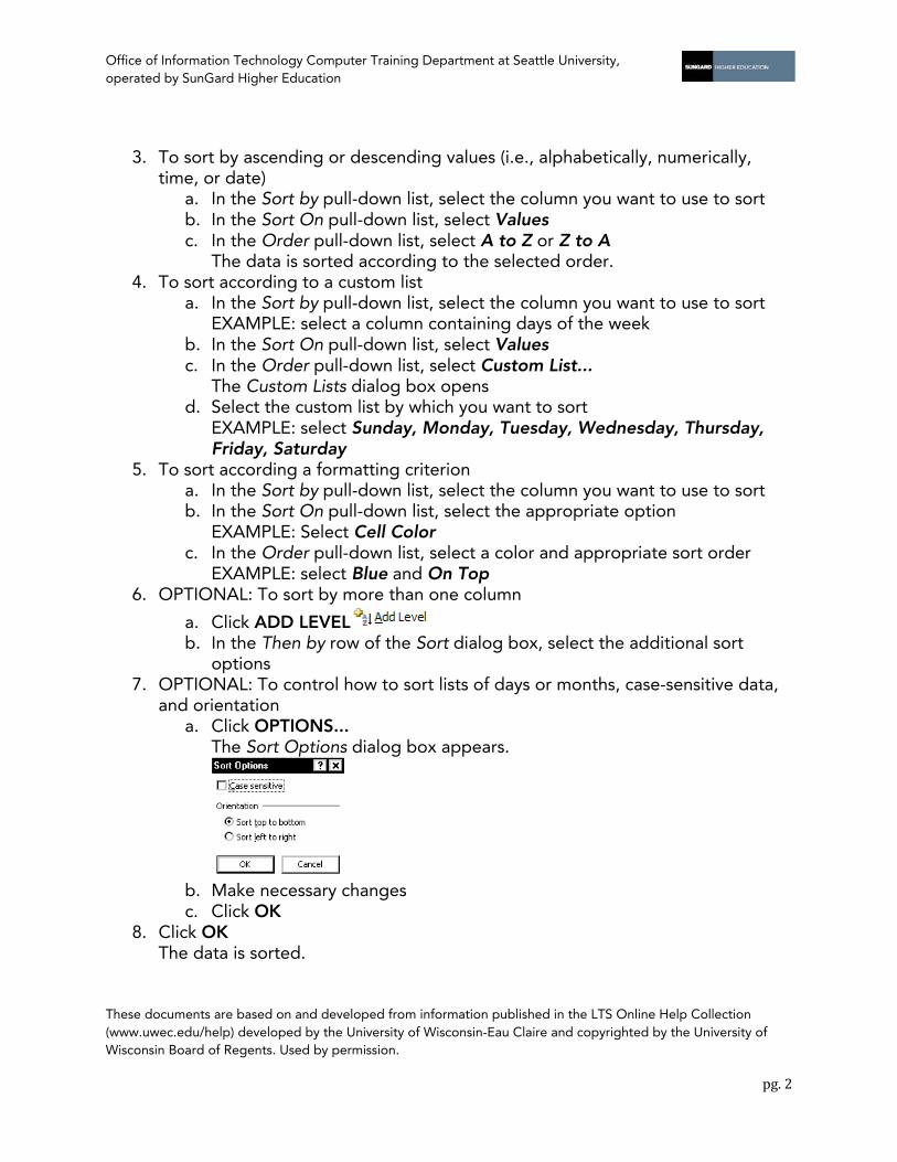
3. To sort by ascending or descending values (i.e., alphabetically, numerically, time, or date)

a. In the Sort by pull-down list, select the column you want to use to sort b. In the Sort On pull-down list, select Values c. In the Order pull-down list, select A to Z or Z to A

The data is sorted according to the selected order. 4. To sort according to a custom list

a. In the Sort by pull-down list, select the column you want to use to sort EXAMPLE: select a column containing days of the week

b. In the Sort On pull-down list, select Values c. In the Order pull-down list, select Custom List...

The Custom Lists dialog box opens d. Select the custom list by which you want to sort

EXAMPLE: select Sunday, Monday, Tuesday, Wednesday, Thursday, Friday, Saturday

5. To sort according a formatting criterion a. In the Sort by pull-down list, select the column you want to use to sort b. In the Sort On pull-down list, select the appropriate option

EXAMPLE: Select Cell Color c. In the Order pull-down list, select a color and appropriate sort order

EXAMPLE: select Blue and On Top 6. OPTIONAL: To sort by more than one column

a. Click ADD LEVEL b. In the Then by row of the Sort dialog box, select the additional sort

options 7. OPTIONAL: To control how to sort lists of days or months, case-sensitive data,

and orientation a. Click OPTIONS...

The Sort Options dialog box appears.

b. Make necessary changes c. Click OK

8. Click OK The data is sorted.



pg. 3

Tables In Excel 2007, a Table is a range of data that can be sorted, filtered, and formatted according to user specifications.

Excel Tables are simple databases, which are stored in Excel workbook files. Excel prefers the term table for its database-like tools and features in order to distinguish them from database applications such as Access. This document provides a basic overview of Tables in Excel 2007.

Table Terms

Excel Tables are made up of columns, column labels, and rows; they can be sorted and/or filtered according to your specifications.

Columns determine the informational structure of table rows NOTE: These are the same as database fields.

Column Labels identify columns; they often have special formatting NOTE: These are the same as database field names.

Rows contain specific data, according to column labels NOTE: These are the same as database records.

AutoFilter button at top of each Table column; provides quick access to sort and filter tools

Sort arranges Table data in order according to text, numbers, time, date, or specific criteria NOTE: Unlike filter, sort displays all table data, but puts them in a specific order.

Filter displays only data meeting criteria you specify (e.g., name, year) NOTE: Unlike sorting, filtering hides some table data, showing only that which fits your criteria.



pg. 4

Tips for Setting Up a Table

There are a few things to consider before creating your Table:

• Columns are the foundation of an Excel Table. Table rows are easy to add and remove, but adding or removing Table columns disrupts a Table's basic structure. To save time and frustration, determine exactly what columns are necessary before creating your Table.

• Do not leave blank rows in the middle of your Table. Blank rows will interfere with Table analysis functions.

• Enter numeric data either as numbers or as text; do not combine the two. HINTS: When using analysis functions, numbers are counted before text. When using mathematical formulas (e.g., SUM and AVERAGE), numbers cannot be entered as text.



pg. 5

Creating Tables Excel Tables are useful for managing sets of related data. Excel 2007 makes it easy to set up a Table and add data to it.

Creating a Table

By creating a table with Excel's Table button, you will have access to Table Tools and the accompanying Design command tab (neither of which are available for normal a data range).

You can either create a blank table or create a table from an existing data range.

Creating a Table: From a Blank Cell Range

1. On your worksheet, select a range of cells you want to make into a Table

2. From the Insert command tab, in the Tables group, click TABLE NOTES: The Create Table dialog box appears, displaying the selected cell range. Behind the Create Table dialog box, the selected cell range is highlighted with an animated border.

3. OPTIONAL: To specify a different cell range, in the Where is the data for your table?

text box, type the desired cell range OR To select the range

a. Click COLLAPSE DIALOG BOX b. Select the desired cell range c. Click EXPAND DIALOG BOX d. Click OK



pg. 6

4. OPTIONAL: If your selected cell range already has headers (i.e., column labels), select My table has headers

5. To accept the selected cell range for your table, click OK The selected cell range is converted into a Table.

Creating a Table: From an Existing Data Range

1. Select the data that will make up your Table

2. From the Insert command tab, in the Tables group, click TABLE The Create Table dialog box appears, displaying the selected data range. If Excel detects headers (i.e., column labels) in the selected data range, the My table has headers option is automatically selected.

3. OPTIONAL: If your table does not already have headers (i.e., column labels), deselect My table has headers

4. OPTIONAL: To specify a different cell range, in the Where is the data for your table? text box, type the desired cell range OR To select the range

a. Click COLLAPSE DIALOG BOX b. Select the desired cell range c. Click EXPAND DIALOG BOX d. Click OK

5. To accept the selected cell range for your Table, click OK The selected cell range is converted into a Table.

To convert a Table back to a data range:

1. Select a cell within the Table 2. From the Design command tab, in the Tools group, click CONVERT TO

RANGE 3. In the confirmation dialog box, click YES

The Table is converted to a range.



pg. 7

Using Forms to Enter Table Data

Once your Table has been created, Excel provides an easy way to enter data called the Form feature. Instead of moving the cursor to each new cell, with the Form feature you can add and edit Table data from a simple dialog box. The Form dialog box is also helpful for searching for records. The Find Next and Find Prev options make locating a specific record easier.

In Excel 2007, to access the Form feature, the Form button must first be added to the Quick Access toolbar.

Adding the Form Button to the Quick Access Toolbar

1. At the top of the Excel window, to the right of the Quick Access toolbar, click CUSTOMIZE QUICK ACCESS TOOLBAR » select More Commands The Excel Options dialog box appears, with Customize selected.

2. From the Customize Quick Access Toolbar section, in the Choose commands from pull-down list, select Commands Not in the Ribbon The scroll box under the pull-down list refreshes to display several commands not found on the Ribbon.

3. From the scroll box, select Form... 4. Click ADD 5. Click OK

The Form button is added to the Quick Access toolbar.

Accessing the Form Dialog Box

NOTES: The Form feature cannot be accessed from a blank worksheet; you must have an existing Table. If you try to open the Form dialog box from empty cell range (i.e., not a Table), a dialog box will appear giving you the option to either use the first row of the selection as labels and not as data (i.e., the Form dialog box opens), or to cancel and make any appropriate changes to your database (i.e., the Form dialog box does not open).

1. Select a cell within the Table 2. From the Quick Access toolbar, click FORM

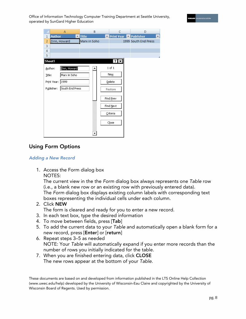
The Form dialog box appears displaying the sheet name, your Table's field names (i.e., column labels), and any previously entered row data. NOTE: The following two graphics depict a Table and the form dialog box when opened from the table.



pg. 8

Using Form Options

Adding a New Record

1. Access the Form dialog box NOTES: The current view in the the Form dialog box always represents one Table row (i.e., a blank new row or an existing row with previously entered data). The Form dialog box displays existing column labels with corresponding text boxes representing the individual cells under each column.

2. Click NEW The form is cleared and ready for you to enter a new record.

3. In each text box, type the desired information 4. To move between fields, press [Tab] 5. To add the current data to your Table and automatically open a blank form for a

new record, press [Enter] or [return] 6. Repeat steps 3–5 as needed

NOTE: Your Table will automatically expand if you enter more records than the number of rows you initially indicated for the table.

7. When you are finished entering data, click CLOSE The new rows appear at the bottom of your Table.



pg. 9

Editing a Record


2. To move to the desired row, click FIND NEXT or FIND PREV OR Press [Up Arrow] or [Down Arrow]

3. In the appropriate Form dialog box text boxes, make the desired changes 4. When finished, click CLOSE

Deleting a Record


2. To select the existing record you want to delete, click and hold the scroll bar dragging up or down OR Click FIND PREV or FIND NEXT

3. Click DELETE A confirmation dialog box appears.

4. Click OK 5. Click CLOSE

The record is permanently deleted from your database.

Searching for a Record

The Criteria feature allows you to search according to desired criteria.


2. Click CRITERIA



pg. 10

3. In the appropriate field(s), type your search criteria 4. Click FIND NEXT or FIND PREV 5. Repeat steps 3-4 as necessary 6. Click CLOSE

Using the Worksheet Window

If you need to make only minor changes in your Table, it may be quicker to make them in the worksheet view.

Adding a Row

1. Click in the first blank row at the bottom of your Table 2. Select the cell where you want to enter new data 3. Type the data accordingly 4. Press [Tab]

OR Use the arrow keys to move to the next field of the record NOTE: As you enter data and move within the row, that row is automatically added to your Table.



pg. 11

Filtering Criteria To perform many of Excel's Table analysis functions, you first need to provide criteria. Criteria is information you provide to relate your Table data with a particular function; it specifies a cell range, a column label, and a condition (e.g., begins with, contains, between).

Criteria can be established to match a single field or multiple fields, multiple conditions (i.e., AND), one of multiple conditions (i.e., OR), or a range of conditions (BETWEEN). Criteria can look for an exact match or a match within specified parameters. Using range names may make database functions easier to write.

Types of Conditions

To properly write criteria, it is important to understand how to format the condition for each criterion. There are three different formats: alphabetic conditions, numeric conditions, and date conditions. The following tables provide the conditions, the correct format, and a sample for each criterion.

Alphabetic Conditions

Condition Format Sample

exact match ="=text_string" ="=john"

begins with text_string john

greater than or equal to

>letter >=letter

>j >=j

less than or equal to

<letter <=letter

<j <=j

between* >letter <letter >j <q

*must be in separate cells within the same row

Numeric Conditions


exact match value 15



pg. 12

contains n/a n/a

greater than or equal to

>value >=value

>15 >=15

less than or equal to

<value <=value

<15 <=15

between* >value <value >15 <25


Date Conditions


one date month/day/year 4/1/1999

contains n/a n/a

date after or equal to

>month/day/year >=month/day/year

>4/1/1999 >=4/1/1999

date before or equal to

<month/day/year <=month/day/year

<4/1/1999 <=4/1/1999

range of dates*

>month/day/year<month/day/year >1/1/1999<12/31/1999


Defining a Single Criterion

A single criterion defines a condition that, when your Table is searched, will return only one type of match for the particular field. The field name goes in the first cell; the condition for that field goes below the field name.

Format Example

column label condition

Pay Period 15



pg. 13

NOTE: In this example, only Table records in which the pay period was equal to 15 would be evaluated for the selected function.

Defining Multiple Criteria

Multiple criteria define conditions that when the database is searched, will return two or more matches. If both conditions must be met, the criteria need to be set up as AND. If a range of conditions must be met, the criteria need to be set up as BETWEEN. However, if only one of multiple conditions must be met, the criteria should be set up as OR.

AND … Match Two Conditions

For "AND" criteria, the fields are within the same row.

Format Example

column label column label 2 condition condition

Pay Period

Student

15 Johnson

NOTE: In this example, only Table records in which the pay period is 15 and the student name contains Johnson would be evaluated for the selected function.

BETWEEN ... Match Two Conditions

For "BETWEEN" criteria, the field is repeated in separate cells within the same row.

Format Example

column label

column label

condition condition

Date Date >3/31/2006 <6/30/2006

NOTE: In this example, only Table records between March 31, 2006 and June 30, 2006 would be evaluated for the selected function.

OR ... Match Either of Two Conditions (Same Field)



pg. 14

For "OR" criteria with the same field, the field criteria are listed in a column under the field name.

Format Example

column label condition condition

Pay Period 15 16

NOTE: In this example, only Table records in which the pay period is 15 or 16 would be evaluated for the selected function.

OR … Match Either of Two Conditions (Different Fields)

For "OR" criteria with different fields, the conditions are listed under the appropriate field name but in separate rows so that they are not treated like "AND" conditions.

Format Example

column label

column label 2

condition condition

Pay Period Student 15 Doe

NOTE: In this example, Table records in which the pay period is 15 or the student name contains Doe would be evaluated for the selected function.



pg. 15

Filtering Your Table Excel 2007 lets you filter Table data according to specific criteria. Any data not matching the specified criteria is hidden from view. Filtered data, however, can be easily viewed again by removing the filter. Filtering is especially useful in large tables when you need to work only with records meeting your precise criteria. This document shows you how to filter Tables in Excel 2007.

Cautions for Working with Filters

When Table filtering is enabled, some Excel commands will produce different results. These can include:

• Cell formatting affects only visible Table cells • When printing the Table, only visible cells will be printed • The Sort command will affect visible cells • When deleting data from the Table, entire rows must be deleted

NOTE: You know filtering is enabled whenever you see the filter buttons at the top of each Table column.

Using Table Filters

The buttons for Table filters are added to each column of your Table. When accessed, they display column-specific pull-down menus from which you can set up a filter. For most Table filtering, this might be all you need. However, when you want to perform more complex filtering, or create a copy of your filtered information, you should use Advanced Filter.

Activating Table Filters

1. Select a cell within the Table

2. From the Home command tab, in the Editing group, click SORT & FILTER » select Filter OR

From the Data command tab, in the Sort & Filter group, click FILTER AutoFilter buttons appear at the top of each column of the selected Table.



pg. 16

Running Table Filters

1. Activate Table Filtering 2. In the column you want to filter, click the

The Table filter pull-down list appears, including a submenu of column-specific records you can use to filter your table. NOTE: By default, all records are selected (i.e., set to display).

3. To filter the selected column, deselect the records you do not want displayed (i.e., be sure that only the records you want displayed are selected)

4. Click OK All rows fitting the criteria of the selected column are displayed. NOTES: When you use AutoFilter within a Table, the row numbers of the displayed records turn blue, and the filter results appear in the status bar (e.g., 1 of 12 records found). The button at the top of the column changes to

5. To remove the filter from your Table, in the filtered column, click the » select Clear Filter From...

Using Custom AutoFilter

Custom AutoFilter allows you to filter a range of information and/or set multiple criteria.

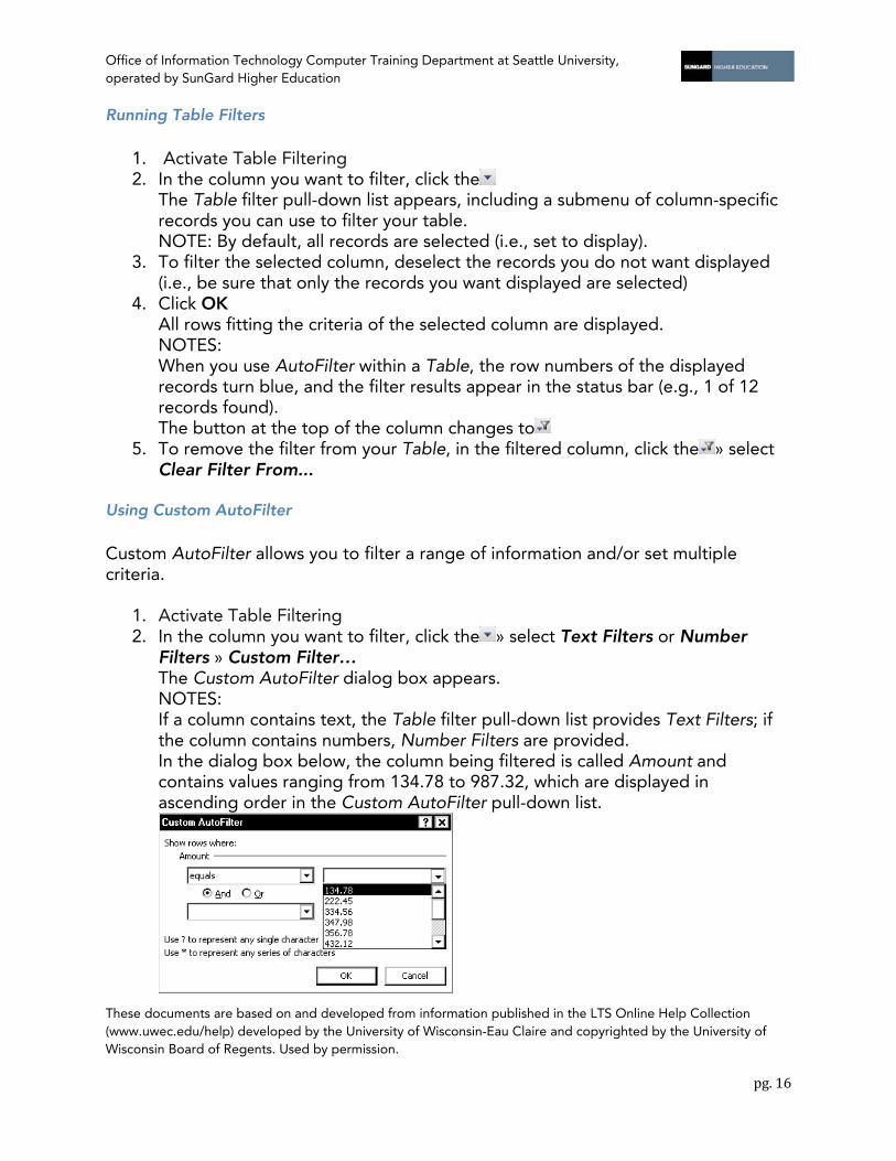
1. Activate Table Filtering 2. In the column you want to filter, click the » select Text Filters or Number

Filters » Custom Filter… The Custom AutoFilter dialog box appears. NOTES: If a column contains text, the Table filter pull-down list provides Text Filters; if the column contains numbers, Number Filters are provided. In the dialog box below, the column being filtered is called Amount and contains values ranging from 134.78 to 987.32, which are displayed in ascending order in the Custom AutoFilter pull-down list.



pg. 17

3. In the Comparison Operator pull-down list, select a type of comparison EXAMPLE: Select is greater than

4. In the Corresponding pull-down list, select or type a criteria value EXAMPLE: Type 300

5. OPTIONAL: If you want multiple criteria, select either And or Or and repeat steps 3 and 4 EXAMPLE: In the Comparison Operator pull-down list, select is less than In the Corresponding pull-down list, type 500

6. Click OK Your Table is filtered to display rows in the selected column containing values between 300 and 500

7. To remove the filter from your Table, in the filtered column, click the » select Clear Filter From...

Turning Off the AutoFilter

1. Select a cell within the Table

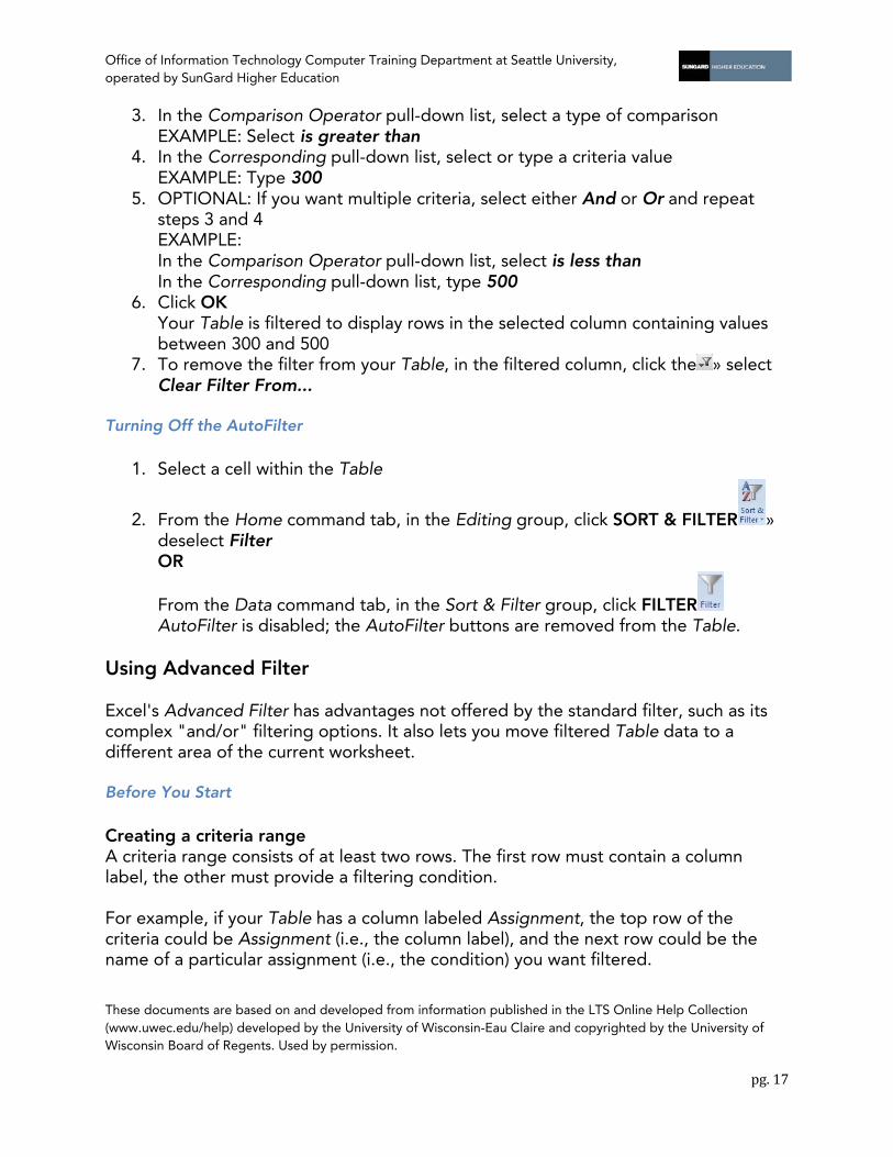
2. From the Home command tab, in the Editing group, click SORT & FILTER » deselect Filter OR

From the Data command tab, in the Sort & Filter group, click FILTER AutoFilter is disabled; the AutoFilter buttons are removed from the Table.

Using Advanced Filter

Excel's Advanced Filter has advantages not offered by the standard filter, such as its complex "and/or" filtering options. It also lets you move filtered Table data to a different area of the current worksheet.

Before You Start

Creating a criteria range A criteria range consists of at least two rows. The first row must contain a column label, the other must provide a filtering condition.

For example, if your Table has a column labeled Assignment, the top row of the criteria could be Assignment (i.e., the column label), and the next row could be the name of a particular assignment (i.e., the condition) you want filtered.



pg. 18

Additional filtering conditions can be established in subsequent rows, allowing you to establish a complex filter. At least one blank row must separate your Table from your criteria range.

Running an Advanced Filter

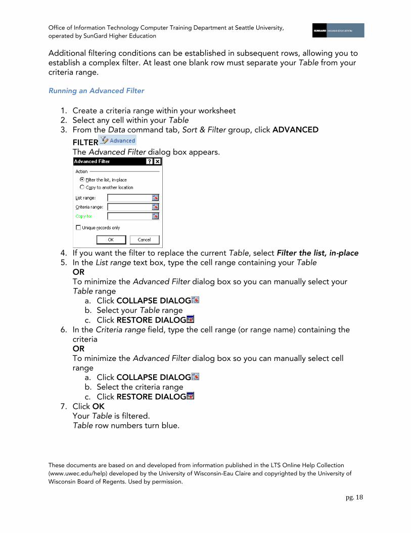
1. Create a criteria range within your worksheet 2. Select any cell within your Table 3. From the Data command tab, Sort & Filter group, click ADVANCED

FILTER The Advanced Filter dialog box appears.

4. If you want the filter to replace the current Table, select Filter the list, in-place 5. In the List range text box, type the cell range containing your Table

OR To minimize the Advanced Filter dialog box so you can manually select your Table range

a. Click COLLAPSE DIALOG b. Select your Table range c. Click RESTORE DIALOG

6. In the Criteria range field, type the cell range (or range name) containing the criteria OR To minimize the Advanced Filter dialog box so you can manually select cell range

a. Click COLLAPSE DIALOG b. Select the criteria range c. Click RESTORE DIALOG

7. Click OK Your Table is filtered. Table row numbers turn blue.



pg. 19

Turning Off Advanced Filter

To remove an Advanced Filter from your Table:

1. From the Data command tab, in the Sort & Filter group, click CLEAR All Table filters are removed.

Copying an Advanced Filter to Another Location

1. Create a criteria range within your worksheet 2. Select a cell within your Table

3. From the Data command tab, click ADVANCED FILTER The Advanced Filter dialog box opens.

4. Select Copy to another location 5. In the List range text box, type the cell range containing your Table

OR To minimize the Advanced Filter dialog box so you can manually select your Table range

a. Click COLLAPSE DIALOG b. Select your Table range c. Click RESTORE DIALOG

6. In the Criteria range field, type the cell range (or range name) containing the criteria OR To minimize the Advanced Filter dialog box so you can manually select the cell range

a. Click COLLAPSE DIALOG b. Select the criteria range c. Click RESTORE DIALOG

7. In the Copy to text box, type a cell or range in the active worksheet where the filter results will appear OR To minimize the Advanced Filter dialog box so you can manually select a cell or range

a. Click COLLAPSE DIALOG b. Select the cell or range c. Click RESTORE DIALOG

8. Click OK



pg. 20

Excel 2007 Sorting, Tables, and Filtering 2007 Sorting, Tables, ... In the Sort by pull-down list,...

Documents

Transcript of Excel 2007 Sorting, Tables, and Filtering 2007 Sorting, Tables, ... In the Sort by pull-down list,...