Evaluation of the Unified Model of the Sphere for Fisheye...
22
This article was downloaded by: [Ecole Centrale de Nantes ] On: 02 February 2013, At: 15:48 Publisher: Taylor & Francis Informa Ltd Registered in England and Wales Registered Number: 1072954 Registered office: Mortimer House, 37-41 Mortimer Street, London W1T 3JH, UK Advanced Robotics Publication details, including instructions for authors and subscription information: http://www.tandfonline.com/loi/tadr20 Evaluation of the Unified Model of the Sphere for Fisheye Cameras in Robotic Applications Jonathan Courbon a , Youcef Mezouar a & Philippe Martinet a a LASMEA, 24 Avenue des Landais, 63171, Aubiere Cedex, France Version of record first published: 24 Jul 2012. To cite this article: Jonathan Courbon , Youcef Mezouar & Philippe Martinet (2012): Evaluation of the Unified Model of the Sphere for Fisheye Cameras in Robotic Applications, Advanced Robotics, 26:8-9, 947-967 To link to this article: http://dx.doi.org/10.1163/156855312X633057 PLEASE SCROLL DOWN FOR ARTICLE Full terms and conditions of use: http://www.tandfonline.com/page/terms-and- conditions This article may be used for research, teaching, and private study purposes. Any substantial or systematic reproduction, redistribution, reselling, loan, sub- licensing, systematic supply, or distribution in any form to anyone is expressly forbidden. The publisher does not give any warranty express or implied or make any representation that the contents will be complete or accurate or up to date. The accuracy of any instructions, formulae, and drug doses should be independently verified with primary sources. The publisher shall not be liable for any loss, actions, claims, proceedings, demand, or costs or damages whatsoever or howsoever caused arising directly or indirectly in connection with or arising out of the use of this material.
Transcript of Evaluation of the Unified Model of the Sphere for Fisheye...
This article was downloaded by: [Ecole Centrale de Nantes ]On: 02 February 2013, At: 15:48Publisher: Taylor & FrancisInforma Ltd Registered in England and Wales Registered Number: 1072954Registered office: Mortimer House, 37-41 Mortimer Street, London W1T 3JH, UK
Advanced RoboticsPublication details, including instructions for authors andsubscription information:http://www.tandfonline.com/loi/tadr20
Evaluation of the Unified Model ofthe Sphere for Fisheye Cameras inRobotic ApplicationsJonathan Courbon a , Youcef Mezouar a & PhilippeMartinet aa LASMEA, 24 Avenue des Landais, 63171, Aubiere Cedex,FranceVersion of record first published: 24 Jul 2012.
To cite this article: Jonathan Courbon , Youcef Mezouar & Philippe Martinet (2012):Evaluation of the Unified Model of the Sphere for Fisheye Cameras in Robotic Applications,Advanced Robotics, 26:8-9, 947-967
To link to this article: http://dx.doi.org/10.1163/156855312X633057
PLEASE SCROLL DOWN FOR ARTICLE
Full terms and conditions of use: http://www.tandfonline.com/page/terms-and-conditions
This article may be used for research, teaching, and private study purposes.Any substantial or systematic reproduction, redistribution, reselling, loan, sub-licensing, systematic supply, or distribution in any form to anyone is expresslyforbidden.
The publisher does not give any warranty express or implied or make anyrepresentation that the contents will be complete or accurate or up to date. Theaccuracy of any instructions, formulae, and drug doses should be independentlyverified with primary sources. The publisher shall not be liable for any loss,actions, claims, proceedings, demand, or costs or damages whatsoever orhowsoever caused arising directly or indirectly in connection with or arising outof the use of this material.
Advanced Robotics 26 (2012) 947–967brill.nl/ar
Full paper
Evaluation of the Unified Model of the Sphere for FisheyeCameras in Robotic Applications
Jonathan Courbon, Youcef Mezouar ∗ and Philippe Martinet
LASMEA, 24 Avenue des Landais, 63171 Aubiere Cedex, France
Received 3 June 2011; accepted 27 June 2011
AbstractA wide field of view is required for many robotic vision tasks. Such an aperture may be acquired by a fisheyecamera, which provides a full image compared to catadioptric visual sensors, and does not increase the sizeand the weakness of the imaging system with respect to perspective cameras. While a unified model existsfor all central catadioptric systems, many different models, approximating the radial distortions, exist forfisheye cameras. It is shown in this paper that the unified projection model proposed for central catadioptriccameras is also valid for fisheye cameras in the context of robotic applications. This model consists of aprojection onto a virtual unitary sphere followed by a perspective projection onto an image plane. This modelis shown equivalent to almost all the fisheye models. Calibration with four cameras and partial Euclideanreconstruction are done using this model, and lead to persuasive results. Finally, an application to a mobilerobot navigation task is proposed and correctly executed along a 200-m trajectory.© Koninklijke Brill NV, Leiden and The Robotics Society of Japan, 2012
KeywordsFisheye camera, projection model, robotics
1. Introduction
Conventional cameras are generally seen as perspective tools (pinhole model),which is convenient for modeling and algorithmic design. Moreover, they exhibitsmall distorsions and thus acquired images can easily be interpreted. Unfortunately,conventional cameras suffer from a restricted field of view. A camera with a largefield of view is useful in many robotic applications including robot localization,navigation and visual servoing. In the literature, several methods have been pro-posed for increasing the field of view. The first method consists on using a movingcamera or a system made of multiple cameras. A second solution consists of com-bining a conventional camera and mirrors. The obtained sensors are referred to as a
* To whom correspondence should be addressed. E-mail: [email protected]
© Koninklijke Brill NV, Leiden and The Robotics Society of Japan, 2012 DOI:10.1163/156855312X633057
Dow
nloa
ded
by [
Eco
le C
entr
ale
de N
ante
s ]
at 1
5:48
02
Febr
uary
201
3

948 J. Courbon et al. / Advanced Robotics 26 (2012) 947–967
Figure 1. Three images acquired approximately at the same position, with a 1/4-inch image sensorwith a perspective lens (left), the same image sensor with an Omnitech Robotics ORIFL190-3 fisheyelens with a field of view of 190° (middle) and a catadioptric camera (right).
catadioptric imaging system. The resulting imaging systems have been termed cen-tral catadioptric when a single projection center describes the world-image mapping[1]. In Ref. [2], a projection model valid for the entire class of central catadioptriccameras has been proposed. According to this generic model, all central catadiop-tric cameras can be modeled by a central projection onto a unitary sphere followedby a perspective projection onto the image plane. Such sensors have been employedin many vision-based robotic applications such as mobile robot localization, navi-gation [3] or visual servoing [4]. However, those cameras exhibit generally a largedead area in the center of the image (Fig. 1, right), which can be a huge drawback.Such sensors also have the drawback of requiring a mirror, which results in a morecumbersome and more fragile sensor imaging system. The last class of cameraswith a wide field of view can be obtained as a dioptric system: a fisheye camera[1]. A fisheye camera is an imaging system that combines a fisheye lens and aconventional camera. Their main advantages with respect to catadioptric sensorsare that (i) they do not exhibit a dead area (Fig. 1, middle) and (ii) a fisheye lensdoes not increase the size and the weakness of the imaging system with respectto a conventional camera. Whereas central catadioptric cameras have a single view-point (central point), fisheye cameras have a locus of projection centers (diacaustic).However, in many robotic applications the small locus could be approximated by asingle viewpoint. As we will see in this paper, the calibration accuracy under thisassumption can satisfy robotic applications.
Fisheye cameras provide an image with a large field of view (around 180° ormore), but exhibit strong distortions. Those distortions are generally split into sev-eral components. The tangential distortions are generally negligible and thus arenot considered here. A decentering distortion is caused by the non-orthogonalityof the lens components with respect to the optical axis [5]. Distortions may alsobe due to the non-regular geometry of the lens. The higher distortions are the ra-dial distortions (barrel or pincushion distortions). Those distortions only dependon the angle of incidence of the incoming ray. Considering robotic applicationssuch as robot navigation or visual servoing, it is reasonable to take into accountonly radial distortions to model fisheye cameras. In this paper, we will use this as-sumption. While a unified model exists for central catadioptric cameras [2], manydifferent models are used for fisheye cameras. The radial distortion models can
Dow
nloa
ded
by [
Eco
le C
entr
ale
de N
ante
s ]
at 1
5:48
02
Febr
uary
201
3

J. Courbon et al. / Advanced Robotics 26 (2012) 947–967 949
be classified into three main groups. The first group is based on the pinhole model.A three-dimensional (3-D) point is first perspectively projected into the image plane(pinhole model). A radial distortion is then applied to the projected point to obtainthe distorted image point. Several parametrical models of distortion can be found inthe literature, such as polynomial-based models [6], logarithmic mapping [7] andhyperbolic cosine mapping [8]. More recently, a parameter-free model has beenproposed in Ref. [9] and used in Ref. [10] for the correction of endoscopic medicalimages. The second category is based on the captured rays. It consists of defininga mapping between the incidence ray direction and the distance between the imagepoint and the image center. Some of these mappings are the f-theta mapping, thestereographic projection [11], the orthogonal projection, the equisolid angle pro-jection and the polynomial model [12]. The last category is based on the unifiedcatadioptric camera model [2, 4]. It is motivated by the fact that similar behaviorshave been observed for those sensors. As has been noted in Ref. [2], the image of3-D straight lines is projected onto conics in the image plane of central catadioptriccameras [4], but also in the image plane of some fisheye cameras [13]. In Ref. [14],a third-order polynomial model of radial distortion is applied to the projected pointobtained with the unified model in order to model central catadioptric cameras andfisheye cameras with the division model of distortions [15]. In Ref. [16], the authorspropose to extend the unified model to include fisheye cameras by substituting theprojection on a sphere by a projection on a quadric surface. In Ref. [17], it is shownthat the division model of radial distortions proposed in Ref. [15] can be describedusing a unitary paraboloid that leads to a geometry similar to paracatadioptric sys-tems.
In this paper, the unified model for catadioptric cameras via a spherical projec-tion (called the unified spherical model (USM)) will be used. This model exhibitsmany advantages. (i) This representation is compact in the sense that a unique pa-rameter will be used to describe radial distortions. (ii) This model is geometricallyintuitive as the sphere provides radial distortions. (iii) The transfer function has ananalytic inverse. (iv) Many algorithms have been designed for central catadioptriccameras using the USM, such as for camera calibration [14], visual servoing [4] orattitude estimation [18]. The aim of this work is to show that the USM can be di-rectly employed to model almost all fisheye cameras. As a consequence, all existingalgorithms for catadioptric cameras are also useful for fisheye lenses.
This paper is organized as follows. In Section 2, the models classically employedfor fisheye cameras are detailled. The USM is presented in Section 3, and validatedfor fisheye cameras in Section 4 through comparison with several existing models,experimental results of calibration and partial Euclidean reconstruction. Section 5reports experimental results in the context of mobile robot navigation using a fish-eye camera. Section 6 presents conclusions.
Dow
nloa
ded
by [
Eco
le C
entr
ale
de N
ante
s ]
at 1
5:48
02
Febr
uary
201
3

950 J. Courbon et al. / Advanced Robotics 26 (2012) 947–967
2. Fisheye Camera Models
Let Fm and Fi be the frames attached to the camera with origin M located at theprojection center and to the image plane with origin I located at the principal point,respectively. Let X be a 3-D point of coordinates X = (X Y Z)T with respect to theframe Fm. The subscripts p and f denote, respectively, perspective and fisheye cam-eras. The perspective image and the fisheye image coordinates of X with respectto Fi are xp = (xp yp)
T and xf = (xf yf)T, respectively. The distance between I
and the image point is denoted by r , the angle between the incoming ray and theprincipal axis by θ (Fig. 2). For a perspective camera, given the focal length f , rpsatisfies:
rp(θ) = f tan θ. (1)
For a fisheye camera, radial distortions have to be taken into account. Manymodels of radial distortions exist, but they respect all the two following fundamentalconstraints:
Constraint 1. The ray arriving along the principal axis is not deformed: rf(0) = 0.
Constraint 2. The radius rf(k) is monotonically increasing for k > 0.
Let us now describe the two families of models classically employed.
2.1. Pinhole-Based Models
The first class of models is based on the pinhole projection. The coordinates of theimage point mf can be obtained thanks to a mapping T1 linking the fisheye and theperspective radii: rp −→T1 rf or by the inverse mapping: rf −→T ′
1rp.
As (1) is not defined for θ = π/2, the models based on the pinhole projection arenot defined too. Those mappings T1 and T ′
1 can be defined by several ways as de-tailed in Table 1(left). In Refs [6, 19] among others, radial distortions are described
Figure 2. Perspective and fisheye imaging process. The perspective image of a 3-D point X is xp andits fisheye image is xf.
Dow
nloa
ded
by [
Eco
le C
entr
ale
de N
ante
s ]
at 1
5:48
02
Febr
uary
201
3

J. Courbon et al. / Advanced Robotics 26 (2012) 947–967 951
Table 1.Models of projection classically employed
Pinhole-based models Captured rays-based models
r1f (rp) = rpL(rp, n) r1
f (θ) = f θ
r2f (rp) = rp
L1(rp,n1)
L2(rp,n2)r2f (θ) = 2f tan( θ
2 )
r3f (rp) = s log(1 + λrp) r3
f (θ) = f sin θ
r4f (θ) = f sin( θ
2 )
r5f (θ) = f (k1θ + k2θ3 + · · · + knθ2(n−1)+1)
r1p (rf) = rf
L(rf,n)r6f (θ) = α sin(βθ)
r2p (rf) = rf
1+k1r2f
r7f (θ) = a tan(θ/b) + c sin(θ/d)
by a polynomial model r1f (rp), where L(rp, n) = 1 + k1r
2p + k2r
4p + · · · + knr
2np .
The n parameters of the model are ki , i = 1,2, . . . , n. This model is classicallyused for perspective cameras [20]. In practice, this model fits to lenses with smalldistortions, but many parameters are needed for lenses with larger distortions. InRef. [21], a piecewise polynomial model of distortion is proposed in order to ob-tain an inverse solution and lower-order polynomials. A rational model r2
f (rp) isproposed in Ref. [22] with n1 + n2 parameters. A logarithmic mapping r3
f (rp) withparameters s (scaling factor) and λ (gain to control the amount of distortion overthe whole image) is used in Ref. [7].
The division model r1p (rf) suggested in Ref. [15] allows us to handle high distor-
tion with few parameters. This model can be used with only one parameter r2p (rf)
[15]. Contrary to the previous models, it is inherently an inverted model in the sensethat it links the distorted radius to the perspective radius.
In Ref. [9], a generic parameter-free model has been proposed. The calibrationstep consists of estimating the position of the distortion center and the discrete val-ues λrp such as rf(rp) = λrp where rf and rp are the distance to the distortion center.The ‘distortion function’ λ = {λ1, λ2, . . . , λn} can be then fitted by a parametricmodel.
2.2. Captured Rays-Based Models
The second group of models is based on captured rays. It consists of defining amapping T2 between the fisheye radius and the incidence angle: θ −→T2 rf.
For perspective cameras, (1) maps the incidence angle θ to the radius r . Forfisheye cameras, this mapping is no longer valid. Some T2-mappings have beenproposed to take into account distortions (refer to Table 1(right), where f is thefocal length of the camera). The f-theta mapping or equiangular or equidistant pro-jection r1
f (θ) proposed in Ref. [23], is suitable for cameras with limited distortions.The stereographic projection r2
f (θ) proposed in Ref. [11] preserves circularity andthus projects 3-D local symmetries onto 2-D local symmetries. The orthogonal or
Dow
nloa
ded
by [
Eco
le C
entr
ale
de N
ante
s ]
at 1
5:48
02
Febr
uary
201
3

952 J. Courbon et al. / Advanced Robotics 26 (2012) 947–967
sine law projection r3f (θ) is described in Ref. [24]. In Ref. [25], the equisolid angle
projection function r4f (θ) is proposed. The polynomial function r5
f (θ) proposed inRefs [12, 26] allows us to improve the accuracy of a polynomial model at the costof increasing the number of parameters. In Ref. [27], the model r6
f (θ) with two pa-rameters α (scale factor) and β (radial mapping parameter) is proposed. The modelr7
f (θ) presented in Ref. [28] is a combination of the stereographic projection (withparameters a, b) with the equisolid angle projection (with parameters c, d).
3. Modeling Fisheye Camera via a Projection on a Sphere
In this section, the USM first is detailed and we then show that it can be viewed as apinhole-based model (Section 3.2) or as a captured rays-based model (Section 3.3).
3.1. World-Image Mapping
As outlined previously, the USM consists of a projection onto a virtual unitarysphere, followed by a perspective projection onto an image plane. This virtual uni-tary sphere is centered in the principal effective view point and the image plane isattached to the perspective camera.
Let Fc and Fm be the frames attached to the conventional camera and to theunitary sphere, respectively. In the sequel, we suppose that Fc and Fm are relatedby a simple translation along the Z-axis (Fc and Fm have the same orientation asdepicted in Fig. 3). The origins C and M of Fc and Fm will be termed optical centerand principal projection center, respectively. The optical center C has coordinates[0 0 −ξ ]T with respect to Fm. The image plane is orthogonal to the Z-axis and it islocated at a distance Z = f from C .
Let X be a 3-D point with coordinates X = [X Y Z]T with respect to Fm. Theworld point X is projected in the image plane into the point of homogeneous coordi-nates x = [x y 1]T. The image formation process can be split in four steps (Fig. 3):
Figure 3. Unified model for a catadioptric camera.
Dow
nloa
ded
by [
Eco
le C
entr
ale
de N
ante
s ]
at 1
5:48
02
Febr
uary
201
3
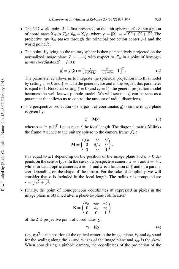
J. Courbon et al. / Advanced Robotics 26 (2012) 947–967 953
• The 3-D world point X is first projected on the unit sphere surface into a pointof coordinates Xm in Fm: Xm = X/ρ, where ρ = ‖X‖ = √
X2 + Y 2 + Z2. Theprojective ray Xm passes through the principal projection center M and theworld point X .
• The point Xm lying on the unitary sphere is then perspectively projected on thenormalized image plane Z = 1 − ξ with respect to Fm in a point of homoge-neous coordinates x′ = f (X):
x′ = f (X) = [X
εsZ+ξρY
εsZ+ξρ1]T
. (2)
The parameter εs allows us to integrate the spherical projection into this modelby setting εs = 0 and ξ = 1. In the general case and in the sequel, this parameteris equal to 1. Note that setting ξ = 0 (and εs = 1), the general projection modelbecomes the well-known pinhole model. We will see that ξ can be seen as aparameter that allows us to control the amount of radial distortions.
• The perspective projection of the point of coordinates x′ onto the image planeis given by:
x = Mx′, (3)
where x = [x y 1]T. Let us note f the focal length. The diagonal matrix M linksthe frame attached to the unitary sphere to the camera frame Fm:
M =(
f κ 0 00 δf κ 00 0 1
).
δ is equal to ±1 depending on the position of the image plane and κ > 0 de-pends on the sensor type. In the case of a perspective camera, κ = 1 and δ = +1,while for catadioptric cameras, δ = −1 and κ is a function of ξ and of a param-eter depending on the shape of the mirror. For the sake of simplicity, we willconsider that κ is included in the focal length. The radius r is computed as:r =√
x2 + y2.
• Finally, the point of homogeneous coordinates m expressed in pixels in theimage plane is obtained after a plane-to-plane collineation
K =(
ku suv u00 kv v00 0 1
)
of the 2-D projective point of coordinates x:
m = Kx. (4)
(u0, v0)T is the position of the optical center in the image plane, ku and kv stand
for the scaling along the x- and y-axes of the image plane and suv is the skew.When considering a pinhole camera, the coordinates of the projection of the
Dow
nloa
ded
by [
Eco
le C
entr
ale
de N
ante
s ]
at 1
5:48
02
Febr
uary
201
3
954 J. Courbon et al. / Advanced Robotics 26 (2012) 947–967
3-D point X in the image plane are obtained setting ξ = 0, κ = 1 and δ = +1.Denoting the focal length fp, we obtain:
{xp = fpX/Z
yp = fpY/Z.(5)
3.1.1. Inverse MappingAn additionnal advantage of the USM is that the transfer function has an analyticinverse. Let Xm be the coordinates vector of the point Xm lying on the unit sphere.Knowing the camera intrinsic parameters, Xm can be computed from the imagepoint x using the relations:
Xm = (η−1 + ξ)x and x = [xT 1
1+ξη
]T, (6)
where:⎧⎪⎨
⎪⎩
η = −γ − ξ(x2 + y2)
ξ2(x2 + y2) − 1
γ =√
1 + (1 − ξ2)(x2 + y2).
We will now show that the model whose final results is given by (3) is equivalentto the pinhole-based model or captured rays-based model.
3.2. Equivalence to the Pinhole-Based Model
By extracting the values of X and Y in (3) and (5), elevating squarely and thentaking the square root, we obtain:
Z + ξρ
ff
√x2
f + y2f︸ ︷︷ ︸
rf
= Z
fp
√x2
p + y2p
︸ ︷︷ ︸rp
. (7)
Noticing that Z > 0, we can write: ρ = Z
√(XZ
)2 + ( YZ
)2 + 1. Thanks to (5), wethus have the relation:
ρ = Z
fp
√r2
p + f 2p . (8)
Then, using (7) we can write:
rf = rf(rp) = (ff/fp)rp
1 + ξ√
r2p/f 2
p + 1. (9)
Equation (9) is a T1-mapping linking the perspective radius rp and the fisheye radiusrf. It can be easily verified that Constraint 1 is respected. Furthermore, since ff, fpand ξ are positive, Constraint 2 is also respected.
Dow
nloa
ded
by [
Eco
le C
entr
ale
de N
ante
s ]
at 1
5:48
02
Febr
uary
201
3

J. Courbon et al. / Advanced Robotics 26 (2012) 947–967 955
3.3. Equivalence to the Captured Rays-Based Model
Using the expressions of x and y given in (2), and noticing that Z + ξρ > 0, we canwrite:
rf =√
x2f + y2
f = ff
Z + ξρ
√X2 + Y 2.
Given that tan θ =√
X2+Y 2
Z, from the previous equation, we deduce:
rf = ff
1 + ξ(ρ/Z)tan θ. (10)
Noticing that ρ can be written as a function of tan θ and Z: ρ = Z√
tan2 θ + 1, (10)can be rewritten:
rf = rf(θ) = ff tan θ
1 + ξ√
tan2 θ + 1. (11)
Equation (11) is clearly a T2-mapping linking the radius rf and the incidence an-gle θ . Once again, it can be easily verified that Constraints 1 and 2 are respected asff and ξ are positive scalars. Note that as usual with the captured rays-based model,the model of the sphere presented in this form is not valid when θ = π/2.
The unified model has been shown to be theoretically equivalent to the mappingsT1 and T2, which implies that it can be used to model fisheye cameras.
4. Validation
In order to validate the USM for fisheye camera, first, the parameters ff and ξ
corresponding to different cameras are computed from the captured rays modelprovided by the camera manufacturers and (11).
In Section 4.2, we show that this model is able to fit almost all existing fisheyecameras. We then calibrate three different visual sensors with a large field of view.Results obtained with the USM are compared to results obtained with other models.The intrinsic parameters of the ORIFL camera are exploited for partial Euclideanreconstruction.
4.1. Fitting Manufacturers Data
Let km be a vector containing the parameters of the projection model m. We willfirst fit the model m with manufacturers data (models i). The estimated parameterskm are obtained using a set of points {(θj , r
if (θj )), j = 1, . . . , n} extracted from the
manufacturer data by solving the following optimization problem:
km = arg minkm
Cm(θ, km),
where the cost function is defined as: Cm(θ, km) =∑nj=1 ‖rm
f (θj , km) − rif (θj )‖.
Dow
nloa
ded
by [
Eco
le C
entr
ale
de N
ante
s ]
at 1
5:48
02
Febr
uary
201
3

956 J. Courbon et al. / Advanced Robotics 26 (2012) 947–967
Figure 4. Plots of model (11) (crosses) fit well with the manufacturers’ data (plain lines).
Table 2.Fitting manufacturers data: mean residual on the nth data multiplied by 1000
rpol2f (θ) r
pol3f (θ) rdiv
p rUSMf (θ)
Coastal Optical 4.88 mm f/5.2 0.6385 0.6287 0.4751 0.6011Nikon MF 6 mm f/2.8 0.5004 0.4286 0.3666 0.4225Coastal Optical 7.45 mm f/2.8 1.7183 1.4344 1.0859 1.5150Sigma 8 mm f/4.0 < 1998 0.9769 0.7797 1.2380 0.7764Peleng 8 mm f/3.5 0.4692 0.4839 0.2695 0.6126Nikkor 10.5 mm f/2.8 1.0395 0.8796 2.3702 0.8481ORIFL190-3 0.1138 0.0757 1.4959 0.0953
Mean 0.7795 0.6730 1.0430 0.6958
We consider data of the captured ray models provided by the manufac-turers of different lenses (Fig. 4). (Data are available on the website: http://michel.thoby.free.fr/Blur_Panorama/Nikkor10-5mm_or_Sigma8mm/Sigma_or_Nikkor/Comparison_Short_Version_Eng.html.) Table 2 summarizes the results ob-tained with four models of fitting m: the polynomial model r3
f (θ) with two param-
eters (rpol2f (θ) = k1θ + k2θ
3) and with three parameters (rpol3f (θ) = k1θ + k2θ
3 +k3θ
5), the division model (rdivp ), and the model of the unitary sphere of (11) (rUSM
f ).A point was set aside during the minimization and then used for validation purposes.For each model m and different lenses, Table 2 shows the mean of the residual errorsobtained with this point put aside.
The smallest residual errors are obtained with the polynomial model rpol3f (using
three parameters). The division model (one parameter) leads to the smallest residualerrors for four lenses, but provides the highest errors for the Sigma, Nikkor andORIFL lenses. The USM gives good results for almost all the lenses with only
Dow
nloa
ded
by [
Eco
le C
entr
ale
de N
ante
s ]
at 1
5:48
02
Febr
uary
201
3
J. Courbon et al. / Advanced Robotics 26 (2012) 947–967 957
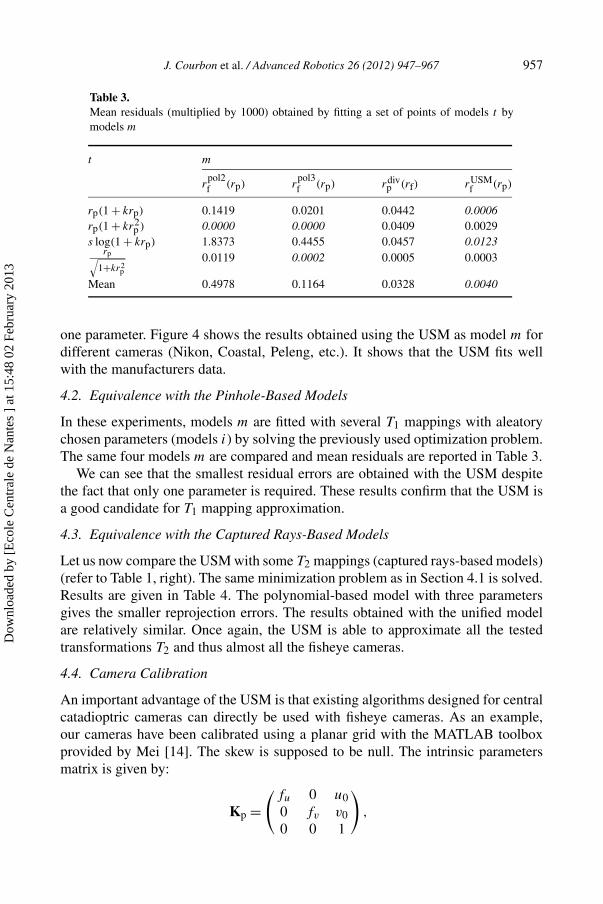
Table 3.Mean residuals (multiplied by 1000) obtained by fitting a set of points of models t bymodels m
t m
rpol2f (rp) r
pol3f (rp) rdiv
p (rf) rUSMf (rp)
rp(1 + krp) 0.1419 0.0201 0.0442 0.0006rp(1 + kr2
p ) 0.0000 0.0000 0.0409 0.0029s log(1 + krp) 1.8373 0.4455 0.0457 0.0123
rp√1+kr2
p
0.0119 0.0002 0.0005 0.0003
Mean 0.4978 0.1164 0.0328 0.0040
one parameter. Figure 4 shows the results obtained using the USM as model m fordifferent cameras (Nikon, Coastal, Peleng, etc.). It shows that the USM fits wellwith the manufacturers data.
4.2. Equivalence with the Pinhole-Based Models
In these experiments, models m are fitted with several T1 mappings with aleatorychosen parameters (models i) by solving the previously used optimization problem.The same four models m are compared and mean residuals are reported in Table 3.
We can see that the smallest residual errors are obtained with the USM despitethe fact that only one parameter is required. These results confirm that the USM isa good candidate for T1 mapping approximation.
4.3. Equivalence with the Captured Rays-Based Models
Let us now compare the USM with some T2 mappings (captured rays-based models)(refer to Table 1, right). The same minimization problem as in Section 4.1 is solved.Results are given in Table 4. The polynomial-based model with three parametersgives the smaller reprojection errors. The results obtained with the unified modelare relatively similar. Once again, the USM is able to approximate all the testedtransformations T2 and thus almost all the fisheye cameras.
4.4. Camera Calibration
An important advantage of the USM is that existing algorithms designed for centralcatadioptric cameras can directly be used with fisheye cameras. As an example,our cameras have been calibrated using a planar grid with the MATLAB toolboxprovided by Mei [14]. The skew is supposed to be null. The intrinsic parametersmatrix is given by:
Kp =(
fu 0 u00 fv v00 0 1
),
Dow
nloa
ded
by [
Eco
le C
entr
ale
de N
ante
s ]
at 1
5:48
02
Febr
uary
201
3

958 J. Courbon et al. / Advanced Robotics 26 (2012) 947–967
Table 4.Mean residuals (multiplied by 1000) obtained by fitting a set of points of models t bymodels m
t m
rpol2f (θ) r
pol3f (θ) rdiv
p rUSMf (θ)
f θ 0.0000 0.0000 0.0405 0.00212f tan( θ
2 ) 0.0058 0.0000 0.0000 0.0000f sin θ 0.0031 0.0000 1.6016 0.0000f sin( θ
2 ) 0.0000 0.0000 0.0105 0.0001k1θ + k2θ3 0.0000 0.0000 0.0594 0.0041
Mean 0.0018 0.0000 0.3424 0.0013
Table 5.Calibration of the ORIFL190-3 of Omnitech Robotics (this camera has a field of view of 190°and a focal length of 1.24 mm; the size of the images is 640 × 480)
Model r1f (rp) USM with distortions USM
Focal length:(fu
fv
) (291.5293.5
) (223.3222.5
) (222.9222.1
)
Principal point:(u0v0
) (315.6255.5
) (305.3266.9
) (305.1266.9
)
Parameters: a =(−0.427
0.142−0.017
)a =
(1.385
−12.860572.772
)ξ = 2.854
ξ = 4.552
Reprojection error:(erruerrv
) (2.0131.933
) (0.1580.132
) (0.1570.141
)
Reprojection error Val.(erruerrv
) (53.81656.798
) (0.1630.136
) (0.1590.142
)
where fu = f · ku and fv = f · kv . [erru, errv] indicates the reprojection errorin pixels. The values prefixed by Val correspond to the error obtained with animage not used during the calibration step. The results of the calibration usingthe pinhole-based model rf(rp) = rp(1 + a1r
2p + · · · + a3r
6p ), the unified model
for central catadioptric cameras (4) with distortions [14] (this model is only pre-sented with fisheye lenses under the division model of distortions r3
f (rp) [15])rf(rc) = rc(1 + a1r
2c + · · · + a3r
6c ) and the model on the sphere are provided in
Table 5 for the ORIFL190-3 of Omnitech Robotics, Table 6 for the Sigma 8/3.5 EXDG of Canon and Table 7 for the Fisheye E5 of Fujinon. The same sets of data havebeen used to calibrate each camera model.
We note that the USM provides satisfactory reprojection errors in all cases. Thedifference compared to the unified model with distortion parameters is small. Using
Dow
nloa
ded
by [
Eco
le C
entr
ale
de N
ante
s ]
at 1
5:48
02
Febr
uary
201
3
J. Courbon et al. / Advanced Robotics 26 (2012) 947–967 959
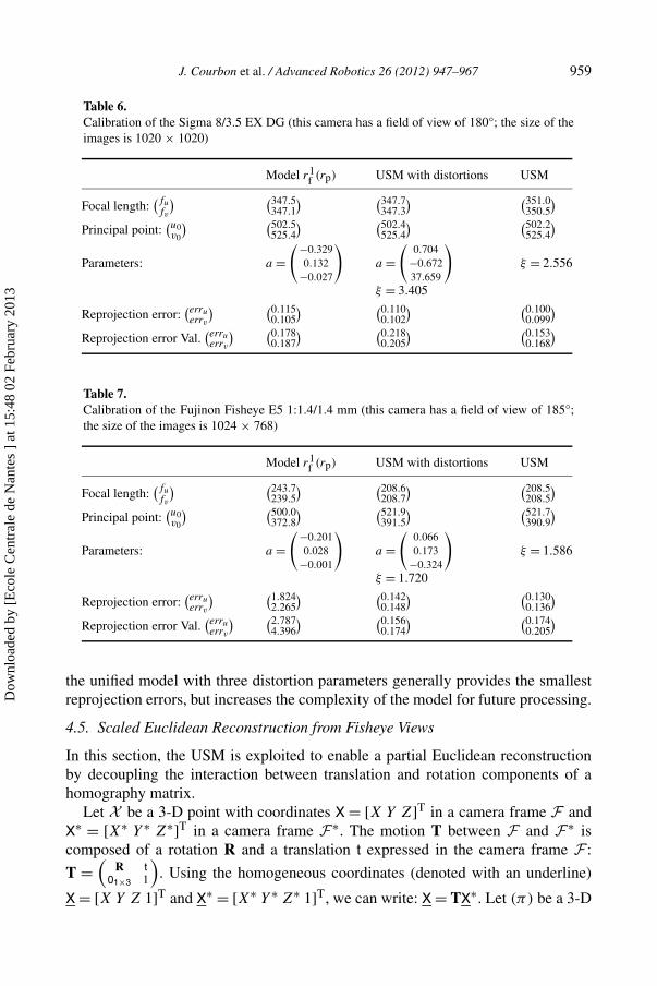
Table 6.Calibration of the Sigma 8/3.5 EX DG (this camera has a field of view of 180°; the size of theimages is 1020 × 1020)
Model r1f (rp) USM with distortions USM
Focal length:(fu
fv
) (347.5347.1
) (347.7347.3
) (351.0350.5
)
Principal point:(u0v0
) (502.5525.4
) (502.4525.4
) (502.2525.4
)
Parameters: a =(−0.329
0.132−0.027
)a =
(0.704
−0.67237.659
)ξ = 2.556
ξ = 3.405
Reprojection error:(erruerrv
) (0.1150.105
) (0.1100.102
) (0.1000.099
)
Reprojection error Val.(erruerrv
) (0.1780.187
) (0.2180.205
) (0.1530.168
)
Table 7.Calibration of the Fujinon Fisheye E5 1:1.4/1.4 mm (this camera has a field of view of 185°;the size of the images is 1024 × 768)
Model r1f (rp) USM with distortions USM
Focal length:(fu
fv
) (243.7239.5
) (208.6208.7
) (208.5208.5
)
Principal point:(u0v0
) (500.0372.8
) (521.9391.5
) (521.7390.9
)
Parameters: a =(−0.201
0.028−0.001
)a =
(0.0660.173
−0.324
)ξ = 1.586
ξ = 1.720
Reprojection error:(erruerrv
) (1.8242.265
) (0.1420.148
) (0.1300.136
)
Reprojection error Val.(erruerrv
) (2.7874.396
) (0.1560.174
) (0.1740.205
)
the unified model with three distortion parameters generally provides the smallestreprojection errors, but increases the complexity of the model for future processing.
4.5. Scaled Euclidean Reconstruction from Fisheye Views
In this section, the USM is exploited to enable a partial Euclidean reconstructionby decoupling the interaction between translation and rotation components of ahomography matrix.
Let X be a 3-D point with coordinates X = [X Y Z]T in a camera frame F andX∗ = [X∗ Y ∗ Z∗]T in a camera frame F ∗. The motion T between F and F ∗ iscomposed of a rotation R and a translation t expressed in the camera frame F :
T =(
R01×3
t1
). Using the homogeneous coordinates (denoted with an underline)
X = [X Y Z 1]T and X∗ = [X∗ Y ∗ Z∗ 1]T, we can write: X = TX∗. Let (π) be a 3-D
Dow
nloa
ded
by [
Eco
le C
entr
ale
de N
ante
s ]
at 1
5:48
02
Febr
uary
201
3

960 J. Courbon et al. / Advanced Robotics 26 (2012) 947–967
reference plane and d(X , π) be the distance from the world point X to the plane(π). This plane is defined by the vector: π∗T = [n∗T − d∗], where n∗ its unitarynormal in F ∗ and d∗ the distance from (π) to the origin of F ∗. If the point Xbelongs to the plane (π ), we can deduce after some algebraic manipulation:
x ∝ Hπx∗, (12)
where Hπ = R + td∗ n∗T is the Euclidean homography matrix related to the plane
(π ), and x and x∗ are computed using (6). Hπ is a function of the camera displace-ment and of the plane coordinates with respect to F ∗. Note that the camera has tobe calibrated to estimate x from the corresponding image points. From the Hπ ma-trix, the camera motion parameters (the rotation matrix R and the scaled translationt/‖t‖) can be estimated using standard homography decomposition [29].
4.5.1. Evaluation with Synthetic ImagesSynthetic images are used to evaluate the performance of the partial 3-D reconstruc-tion using the USM (Fig. 5). The camera is placed in the virtual working space,looking to a plane π containing N points aleatory located. The 640 × 480 syn-thetic images are generated by projecting those points in the image plane using theprojection model r1
f (rp) with the parameters of the ORIFL found in Section 4.4(i.e., r1
f (rp) = rp(1 − 0.238r2p + 0.040r4
p + 0.002r6p − 0.001r8
p )). Two-dimensionalGaussian noise with zero mean and standard deviation σ is added to each imagepoint. For each experiment, two positions of the camera are aleatory generated witha displacement consisting of the rotation R and the translation t. The homographymatrix Hπ related to the plane π between the two images is estimated for the USMwith parameters of the ORIFL lens (i.e., ξ = 2.875).
Figure 5. Geometry of two views.
Dow
nloa
ded
by [
Eco
le C
entr
ale
de N
ante
s ]
at 1
5:48
02
Febr
uary
201
3

J. Courbon et al. / Advanced Robotics 26 (2012) 947–967 961
Figure 6. Partial Euclidean reconstruction with synthetic data: r.m.s. errors (in rad) using 6, 10, 20and 40 points in correspondences versus standard deviation σ = 0, . . . ,2 pixel(s). Plain lines, USM;dashed lines, perspective projection.
The estimated rotation R and scaled translation t are then extracted from Hπ .Two errors are computed. The rotational error is the rotation angle �R of the matrixRR−1 and the translational error is the angle �T between the normalized vectorst/‖t‖ and t/‖t‖. In order to compare with the well-known perspective case, the ho-mography matrix Hπ is also estimated with the pinhole projection model used togenerate the images. Rotation and translation are extracted from Hπ , and rotationaland translational errors are computed. The results are compared with the groundtruth and the root mean square (r.m.s.) error is computed over 200 runs of eachexperiment (Fig. 6).
Figure 6 shows that the results are similar to those obtained with a perspectivecamera: the r.m.s. error is increasing when the standard deviation increases and isdecreasing when the number of points used to compute the homography matrixincreases. Moreover, for a small number of points, the error of reconstruction withthe USM is better than that obtained with a pinhole model. As expected, withoutnoise, values of the errors are zero when the same (perspective) projection modelhas been used for image generation and homography computation, and are not nullwhen images are generated with the pinhole model and homography matrices arecomputed with the USM.
4.5.2. Experiments with Real DataThree camera displacements have been considered: translation t, rotation R, androtation and translation (R, t) (Table 8). These displacements are estimated by usingthe images acquired by the ORIFL190-3 fisheye camera (calibrated as explainedin Section 4.4) at the initial and final positions by decomposing the homographymatrix (rotation matrix R and normalized translation t/‖t‖).
As observed in Table 8, displacements are well estimated. When a translation isrealized, an error of less than 1° is observed. The error between the computed rota-
Dow
nloa
ded
by [
Eco
le C
entr
ale
de N
ante
s ]
at 1
5:48
02
Febr
uary
201
3

962 J. Courbon et al. / Advanced Robotics 26 (2012) 947–967
Table 8.Three-dimensional partial reconstruction with real data: computation of the displacement:translation, rotation, and rotation and translation (the rotation is represented by uθ (rotationaxis u and angle θ expressed in deg))
Translation Rotation
t/‖t‖ (m) 0.843 −0.334 0.422 uθ (deg) 0 −40.00 0t/‖t‖ (m) 0.841 −0.344 0.417 uθ (deg) 0.206 −39.4 −3.20
�T (deg) 0.917 �R (deg) 3.20
Translation and rotationt/‖t‖ (m) 0.688 0 0.726 uθ (deg) 0 −20.00 0t/‖t‖ (m) 0.673 −0.015 0.740 uθ (deg) 0.470 −21.77 −0.006
�T (deg) 1.21 �R (deg) 1.831
tion and the real rotation is about 3°. When a rotation and translation displacementis realized, the errors are less than 2°.
5. Navigation of a Non-Holonomic Vehicle with a Fisheye Camera
Many vision-based navigation strategies are emerging [30, 31] and may benefit fora large field-of-view camera to be more robust to occlusions. In this section, thevision-based navigation framework for a non-holonomic mobile robot presented inRef. [32] with central cameras is extended to fisheye cameras. Principles of thenavigation framework are briefly presented in Section 5.1. Experiments with thefisheye camera are presented in Section 5.2.
5.1. Vision-Based Navigation
The framework consists on two successive steps. During an off-line learning step,the robot performs paths that are sampled and stored as a set of ordered key imagesacquired by the embedded fisheye camera. The set of visual paths can be interpretedas a visual memory of the environment. In the second step, the robot is controlledby a vision-based control law along a visual route that joins the current image tothe target image in the visual memory.
To design the controller, the key images of the reference visual route are consid-ered as consecutive checkpoints to reach in the sensor space. The robot is controlledfrom the image Ii to the next image of the visual route Ii+1. The control problemcan be formulated as a path following to guide the non-holonomic mobile robotalong the visual route.
Let us note Fi = (Oi,Xi,Yi,Zi) and Fi+1 = (Oi+1,Xi+1,Yi+1,Zi+1) theframes attached to the robot when Ii and Ii+1 were stored, and Fc = (Oc,Xc,Yc,
Zc) a frame attached to the robot in its current location. Figure 7 illustrates thissetup.
Dow
nloa
ded
by [
Eco
le C
entr
ale
de N
ante
s ]
at 1
5:48
02
Febr
uary
201
3
J. Courbon et al. / Advanced Robotics 26 (2012) 947–967 963
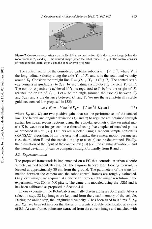
Figure 7. Control strategy using a partial Euclidean reconstruction. Ic is the current image (when therobot frame is Fc) and Ii+1 the desired image (when the robot frame is Fi+1). The control consistsof regulating the lateral error y and the angular error θ to zero.
The control vector of the considered cart-like robot is u = [V ω]T, where V isthe longitudinal velocity along the axle Yc of Fc and ω is the rotational velocityaround Zc. Consider the straight line � = (Oi+1,Yi+1) (Fig. 7). The control strat-egy consists in guiding Ic to Ii+1 by regulating asymptotically the axle Yc on �.The control objective is achieved if Yc is regulated to � before the origin of Fc
reaches the origin of Fi+1. Let θ be the angle (around the axle Z) between Fc
and Fi+1 and y the distance between Oc and �. We use the asymptotically stableguidance control law proposed in [32]:
ω(y, θ) = −V cos3 θKpy − |V cos3 θ |Kd tan θ, (13)
where Kp and Kd are two positive gains that set the performances of the controllaw. The lateral and angular deviations (y and θ ) to regulate are obtained throughpartial Euclidean reconstructions using the epipolar geometry. The essential ma-trix E between two images can be estimated using five couples of matched pointsas proposed in Ref. [33]. Outliers are rejected using a random sample consensus(RANSAC) algorithm. From the essential matrix, the camera motion parameters(i.e., the rotation R and the translation t up to a scale) can be determined. Finally,the estimation of the input of the control law (13) (i.e., the angular deviation θ andthe lateral deviation y) can be computed straightforwardly from R and t.
5.2. Experimentation
The proposed framework is implemented on a PC that controls an urban electricvehicle, named RobuCab (Fig. 8). The Fujinon fisheye lens, looking forward, islocated at approximately 80 cm from the ground. The parameters of the transfor-mation between the camera and the robot control frames are roughly estimated.Grey level images are acquired at a rate of 15 frames/s. The image resolution in theexperiments was 800 × 600 pixels. The camera is modeled using the USM and ithas been calibrated as proposed in Section 4.4.
In our experiment, the RobuCab is manually driven along a 200-m path. After aselection step, 82 key images are kept and form the visual memory of the vehicle.During the online step, the longitudinal velocity V has been fixed to 0.8 ms−1. Kpand Kd have been set in order that the error presents a double pole located at a valueof 0.3. At each frame, points are extracted from the current image and matched with
Dow
nloa
ded
by [
Eco
le C
entr
ale
de N
ante
s ]
at 1
5:48
02
Febr
uary
201
3

964 J. Courbon et al. / Advanced Robotics 26 (2012) 947–967
Figure 8. RobuCab vehicle with the embedded fisheye camera.
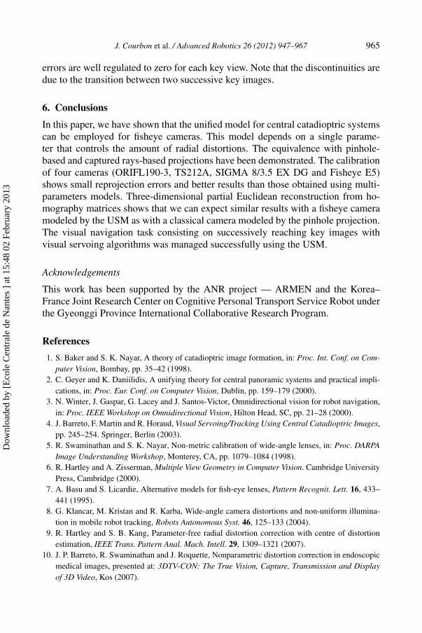
Figure 9. Lateral y (m, up to a scale factor) and angular θ errors (rad) and control input δ (rad) versustime (s).
the desired key image. These points are exploited to compute the rotation and thetranslation between the current and the desired key images. Angular and lateralerrors are extracted and used as input of the control law (13).
The RobuCab successfully follows the visual path to reach its target. A mean of105 good matches for each frame has been found. The mean computational timeduring the online navigation was of 72 ms by image. For the state estimation, themean reprojection error in the three views was around 2.5 pixels. Lateral and angu-lar errors as well as control input are represented in Fig. 9. As can be seen, those
Dow
nloa
ded
by [
Eco
le C
entr
ale
de N
ante
s ]
at 1
5:48
02
Febr
uary
201
3
J. Courbon et al. / Advanced Robotics 26 (2012) 947–967 965
errors are well regulated to zero for each key view. Note that the discontinuities aredue to the transition between two successive key images.
6. Conclusions
In this paper, we have shown that the unified model for central catadioptric systemscan be employed for fisheye cameras. This model depends on a single parame-ter that controls the amount of radial distortions. The equivalence with pinhole-based and captured rays-based projections have been demonstrated. The calibrationof four cameras (ORIFL190-3, TS212A, SIGMA 8/3.5 EX DG and Fisheye E5)shows small reprojection errors and better results than those obtained using multi-parameters models. Three-dimensional partial Euclidean reconstruction from ho-mography matrices shows that we can expect similar results with a fisheye cameramodeled by the USM as with a classical camera modeled by the pinhole projection.The visual navigation task consisting on successively reaching key images withvisual servoing algorithms was managed successfully using the USM.
Acknowledgements
This work has been supported by the ANR project — ARMEN and the Korea–France Joint Research Center on Cognitive Personal Transport Service Robot underthe Gyeonggi Province International Collaborative Research Program.
References
1. S. Baker and S. K. Nayar, A theory of catadioptric image formation, in: Proc. Int. Conf. on Com-puter Vision, Bombay, pp. 35–42 (1998).
2. C. Geyer and K. Daniilidis, A unifying theory for central panoramic systems and practical impli-cations, in: Proc. Eur. Conf. on Computer Vision, Dublin, pp. 159–179 (2000).
3. N. Winter, J. Gaspar, G. Lacey and J. Santos-Victor, Omnidirectional vision for robot navigation,in: Proc. IEEE Workshop on Omnidirectional Vision, Hilton Head, SC, pp. 21–28 (2000).
4. J. Barreto, F. Martin and R. Horaud, Visual Servoing/Tracking Using Central Catadioptric Images,pp. 245–254. Springer, Berlin (2003).
5. R. Swaminathan and S. K. Nayar, Non-metric calibration of wide-angle lenses, in: Proc. DARPAImage Understanding Workshop, Monterey, CA, pp. 1079–1084 (1998).
6. R. Hartley and A. Zisserman, Multiple View Geometry in Computer Vision. Cambridge UniversityPress, Cambridge (2000).
7. A. Basu and S. Licardie, Alternative models for fish-eye lenses, Pattern Recognit. Lett. 16, 433–441 (1995).
8. G. Klancar, M. Kristan and R. Karba, Wide-angle camera distortions and non-uniform illumina-tion in mobile robot tracking, Robots Autonomous Syst. 46, 125–133 (2004).
9. R. Hartley and S. B. Kang, Parameter-free radial distortion correction with centre of distortionestimation, IEEE Trans. Pattern Anal. Mach. Intell. 29, 1309–1321 (2007).
10. J. P. Barreto, R. Swaminathan and J. Roquette, Nonparametric distortion correction in endoscopicmedical images, presented at: 3DTV-CON: The True Vision, Capture, Transmission and Displayof 3D Video, Kos (2007).
Dow
nloa
ded
by [
Eco
le C
entr
ale
de N
ante
s ]
at 1
5:48
02
Febr
uary
201
3

966 J. Courbon et al. / Advanced Robotics 26 (2012) 947–967
11. M. M. Fleck, Perspective projection: the wrong imaging model, Technical report 95-01, ComputerScience, University of Iowa, Ames, IA (1994).
12. Y. Xiong and K. Turkowski, Creating image-based VR using a self-calibrating fisheye lens, in:Proc. Conf. on Computer Vision and Pattern Recognition, Puerto Rico, p. 237 (1997).
13. P. W. Smith, K. B. Johnson and M. A. Abidi, Efficient techniques for wide-angle stereo vision us-ing surface projection models, in: Proc. IEEE Conf. on Computer Vision and Pattern Recognition,Fort Collins, CO, vol. 1, pp. 113–118 (1999).
14. C. Mei and P. Rives, Single view point omnidirectional camera calibration from planar grids, in:Proc. IEEE Int. Conf. on Robotics and Automation, Rome, pp. 3945–3950 (2007).
15. A. Fitzgibbon, Simultaneous linear estimation of multiple-view geometry and lens distortion, in:Proc. IEEE Conf. on Computer Vision and Pattern Recognition, Maui, HI, vol. 1, pp. I-125–I-132(2001).
16. X. Ying and Z. Hu, Can we consider central catadioptric cameras and fisheye cameras withina unified imaging model, in: Proc. Eur. Conf. on Computer Vision, Prague, vol. I, pp. 442–455(2004).
17. J. P. Barreto, A unifying geometric representation for central projection systems, Comp. Vis. ImageUnderstand. 103, 208–217 (2006).
18. J.-C. Bazin, I. So Kweon, C. Demonceaux and P. Vasseur, UAV attitude estimation by combin-ing horizon-based and homography-based approaches for catadiopric images, in: Proc. 6th IFACSymposium on Intelligent Autonomous Vehicles, Toulouse (2007).
19. T. Pajdla, T. Werner and V. Hlavác, Correcting radial lens distortion without knowledge of 3-Dstructure, Technical Report K335-CMP-1997-138, Czech Technical University (1997).
20. Z. Zhang, A flexible new technique for camera calibration, Technical Report MSR-TR-98-71, Mi-crosoft Research (1998).
21. L. Ma, Y. Chen and K. L. Moore, Analytical piecewise radial distortion model for precision cameracalibration, Vision Image Signal Process. 153, 468–474 (2006).
22. H. Li and R. Hartley, An easy non-iterative method for correcting lens distortion from nine pointcorrespondences, presented at: Workshop on Omnidirectional Vision, Camera Networks and Non-classical Cameras, Beijing (2005).
23. R. Kingslake, A History of the Photographic Lens. Academic Press, San Diego, CA (1989).24. S. F. Ray, Applied Photographic Optics, 2nd edn. Focal Press, Oxford (1994).25. W. J. Smith, Modern Lens Design: A Resource Manual. McGraw-Hill, New York, NY (1992).26. E. Schwalbe, Geometric modelling and calibration of fisheye lens camera systems, presented at:
ISPRS Panoramic Photogrammetry Workshop, Berlin (2005).27. J. Kumler and M. Bauer, Fisheye lens designs and their relative performance, SPIE 4093, 360–369
(2000).28. H. Bakstein and T. Pajdla, Panoramic mosaicing with a 180° field of view lens, in: Proc. IEEE
Workshop on Omnidirectional Vision, Los Alamitos, CA, pp. 60–67 (2002).29. O. Faugeras and F. Lustman, Motion and structure from motion in a piecewise planar environment,
Int. J. Pattern Recognit. Artif. Intell. 2, 485–508 (1988).30. T. Goedemé, T. Tuytelaars, G. Vanacker, M. Nuttin, L. Van Gool and L. Van Gool, Feature based
omnidirectional sparse visual path following, in: Proc. IEEE/RSJ Int. Conf. on Intelligent Robotsand Systems, Edmonton, pp. 1806–1811 (2005).
31. A. Diosi, A. Remazeilles, S. Segvic and F. Chaumette, Outdoor visual path following experiments,in: Proc. IEEE/RSJ Int. Conf. on Intelligent Robots and Systems, San Diego, CA, pp. 4265–4270(2007).
Dow
nloa
ded
by [
Eco
le C
entr
ale
de N
ante
s ]
at 1
5:48
02
Febr
uary
201
3

J. Courbon et al. / Advanced Robotics 26 (2012) 947–967 967
32. J. Courbon, G. Blanc, Y. Mezouar and P. Martinet, Navigation of a non-holonomic mobile robotwith a memory of omnidirectional images, presented at: ICRA 2007 Workshop on ‘Planning, Per-ception and Navigation for Intelligent Vehicles’, Rome (2007).
33. D. Nistér, An efficient solution to the five-point relative pose problem, Trans. Pattern Anal. Mach.Intell. 26, 756–770 (2004).
About the Authors
Jonathan Courbon graduated from the Institut Français de Mécanique Avancée(IFMA), Clermont-Ferrand, France, in 2005. He received the PhD degree in Vi-sion and Robotics from the Université Blaise Pascal, Clermont-Ferrand, in 2009.He is now pursuing his Postdoc at the Robotics and Vision Group of LASMEA-CNRS, Clermont-Ferrand. His research focuses on the use of visual informationsfor navigation and control of mobile robots.
Youcef Mezouar received the PhD degree in Computer Science from the Uni-versité de Rennes 1, Rennes, France, in 2001, and the ‘Habilitation à Dirigerles Recherches’ degree from the Université Blaise Pascal, Clermont-Ferrand,France, in 2009. For 1 year, he was a Postdoctoral Associate with the RoboticsLaboratory, Computer Science Department, Columbia University, New York. In2002, he joined the Robotics and Vision Group, LASMEA-CNRS, Blaise Pas-cal University, where he is currently a Colead of the GRAVIR Group (http://www.lasmea.univ-bpclermont.fr) and the ROSACE Team (http://www.lasmea.
univ-bpclermont.fr/rosace). His research interests include automatics, robotics and computer vision,especially visual servoing and mobile robot navigation.
Philippe Martinet graduated from the CUST, Clermont-Ferrand, France, in 1985,and he received the PhD degree in Electronics Science from the Blaise PascalUniversity, Clermont-Ferrand, in 1987. From 1990 to 2000, he was Assistant Pro-fessor with CUST in the Electrical Engineering Department, Clermont-Ferrand.From 2000 to 2011, he was Professor with Institut Français de Mécanique Avancée(IFMA), Clermont-Ferrand. He was performing research at the Robotics and Vi-sion Group of LASMEA-CNRS, Clermont-Ferrand. In 2006, he spent 1 year asa Visiting Professor in ISRC at the Sungkyunkwan University in Suwon, South
Korea. In 2011, he moved to Ecole Centrale de Nantes and he is doing research at IRCCYN. He wasthe Leader of the group GRAVIR (over 74 persons) from 2001 to 2006. In 1999, he set up a teamin Robotics and Autonomous Complex Systems (over 20 persons). Between 2008 and 2011, he wasColead of a Joint Unit of Technology called ‘Robotization Meets Industry’. Between 2009 and 2011,he was Colead of a Korea–France Joint Research Center on Cognitive Personal Transport ServiceRobots. His research interests include visual servoing of robots (position, image and hybrid based,omnidirectional), multi-sensor-based control, force–vision coupling), autonoumous guided vehicles(control, enhanced mobility, uncertain dynamics, monitoring), modeling, identification and control ofcomplex machines (vision-based kinematic/dynamic modeling identification and control). From 1990,he is Author and Coauthor of more than two hundred thirty references.
Dow
nloa
ded
by [
Eco
le C
entr
ale
de N
ante
s ]
at 1
5:48
02
Febr
uary
201
3