EVALUATION OF THE SIGNALISED JUNCTION PERFORMANCE AT …
87
EVALUATION OF THE SIGNALISED JUNCTION PERFORMANCE AT JALAN PONTIAN LAMA-PULAI SKUDAI, JOHOR MUHAMAD HAFIZ BIN MOHAMAD RIZAL UNIVERSITI TEKNOLOGI MALAYSIA
Transcript of EVALUATION OF THE SIGNALISED JUNCTION PERFORMANCE AT …

EVALUATION OF THE SIGNALISED JUNCTION PERFORMANCE AT JALAN
PONTIAN LAMA-PULAI SKUDAI, JOHOR
MUHAMAD HAFIZ BIN MOHAMAD RIZAL
UNIVERSITI TEKNOLOGI MALAYSIA

NOTES : If the thesis is CONFIDENTIAL or RESTRICTED, please attach with the letter from the organization with period and reasons for confidentiality or restriction
PSZ 19:16 (Pind. 1/13)
UNIVERSITI TEKNOLOGI MALAYSIA
DECLARATION OF THESIS / UNDERGRADUATE PROJECT REPORT AND
COPYRIGHT Author’s full name : Muhamad Hafiz Bin Mohamad Rizal Date of Birth : 27 August 1996
Title : Evaluation of the Signalised Junction Performance at Jalan Pontian Lama-Pulai Skudai, Johor
Academic Session : 2018/2019 I declare that this thesis is classified as:
CONFIDENTIAL (Contains confidential information under the Official Secret Act 1972)*
RESTRICTED (Contains restricted information as specified by the organization where research was done)*
✓ OPEN ACCESS I agree that my thesis to be published as online open access (full text)
1. I acknowledged that Universiti Teknologi Malaysia reserves the right as
follows:
2. The thesis is the property of Universiti Teknologi Malaysia
3. The Library of Universiti Teknologi Malaysia has the right to make copies for
the purpose of research only.
4. The Library has the right to make copies of the thesis for academic
exchange.
Certified by:
SIGNATURE OF STUDENT SIGNATURE OF SUPERVISOR
960827-02-6339 IR. DR. SITTI ASMAH BINTI
HASSAN
MATRIX NUMBER NAME OF SUPERVISOR
Date: 23 MAY 2019 Date: 23 MAY 2019


“I hereby declare that I have read this project report and in my
opinion this project report is sufficient in terms of scope and quality for the
award of the degree of Bachelor of Civil Engineering”
Signature : ________________________________
Name of Supervisor : IR. DR. SITTI ASMAH BINTI HASSAN
Date : 23 MAY 2019

BAHAGIAN A - Pengesahan Kerjasama*
Adalah disahkan bahawa projek penyelidikan tesis ini telah dilaksanakan melalui
kerjasama antara ________________________dengan ________________________
Disahkan oleh:
Tandatangan : Tarikh :
Nama :
Jawatan :
(Cop rasmi)
* Jika penyediaan tesis atau projek melibatkan kerjasama.
BAHAGIAN B - Untuk Kegunaan Pejabat Sekolah Pengajian Siswazah
Tesis ini telah diperiksa dan diakui oleh:
Nama dan Alamat Pemeriksa Luar :
Nama dan Alamat Pemeriksa Dalam :
Nama Penyelia Lain (jika ada) :
Disahkan oleh Timbalan Pendaftar di SPS:
Tandatangan : Tarikh : 15JULAI 2018
Nama :


EVALUATION OF THE SIGNALISED JUNCTION PERFORMANCE AT JALAN
PONTIAN LAMA-PULAI SKUDAI, JOHOR
MUHAMAD HAFIZ BIN MOHAMAD RIZAL
A project report submitted in fulfilment of the
requirements for the award of the degree of
Bachelor of Civil Engineering
School of Civil Engineering
Faculty of Engineering
Universiti Teknologi Malaysia
MAY 2019


i
DECLARATION
I declare that this project report entitled “Evaluation Of The Signalised Junction
Performance At Jalan Pontian Lama-Pulai Skudai, Johor” is the result of my own
research except as cited in the references. The project report has not been accepted for
any degree and is not concurrently submitted in candidature of any other degree.
Signature : ....................................................
Name : MUHAMAD HAFIZ BIN MOHAMAD RIZAL
Date : 23 MAY 2019
ii
DEDICATION
To my beloved family.
Thank you all the support and encouragement.
To my supervisor, Ir. Dr. Sitti Asmah Binti Hassan
Thank you for your guidance, advice and support given in completing this study.
To all my follow friends who assist me in completing this study.
For all your assistance and support will always be remembered.

iii
ACKNOWLEDGEMENT
First and foremost, all grateful and thanks to Allah SWT, the Lord of Universe,
the most gracious and merciful on blessing.
Thanks a lot to my supervisor Ir. Dr. Sitti Asmah Binti Hassan for her guidance,
advice and precious supervision
Also, tribute all appreciation goes to my parent, Rizal and Roslina for their
support, wish and sacrifice directly or indirectly towards the end. Finally, to all my
friends, thanks for all moments.

iv
ABSTRACT
Road network is really important in human daily use as they use it to access
from place to place. It is really important to make an assessment on road performance
as to keep the traffic moving as smoothly as possible. In Jalan Pontian Lama-Pulai,
drivers in the area of signalised junction have to wait longer before given a green
indication. This study aims to evaluate junction performance at signalised junction in
Jalan Pontian Lama-Pulai. Traffic volume and signal indication at the junction were
obtained for one weekday during peak hour from 7am to 9am, 12pm to 2pm and 5pm
to 7pm. The data was collected using manual counting technique and video recording
method. Morning peak volume was used in analysing LOS. The data was analysed to
obtain stopped delay using guidelines in Arahan Teknik Jalan 13/87. In this study it
was found that traffic directions of the signalised junction experienced level of service
in a range of C to E that indicates unstable flow. It was suggested that cycle time of
the signal system at the junction was redesign to a shorter cycle time 60 second.

v
ABSTRAK
Rangkaian jalan sangat penting dalam penggunaan harian manusia kerana
penggunaannya untuk bergerak dari satu tempat ke tempat. Membuat penilaian
terhadap prestasi jalan adalah sangat penting bagi memastikan lalu lintas bergerak
selancar yang mungkin. Di Jalan Pontian Lama-Pulai, pemandu di kawasan simpang
yang mempunyai lampu isyarat perlu menunggu lebih lama sebelum fasa lampu hijau.
Kajian ini bertujuan untuk menilai prestasi di simpang berisyarat di Jalan Pontian
Lama-Pulai. Jumlah lalu lintas dan petunjuk isyarat di simpang diperolehi untuk satu
hari kerja pada waktu puncak dari jam 7 pagi hingga 9 pagi, 12 malam hingga 2 petang
dan 5 petang hingga 7 malam. Pengumpulan data bagi kajian adalah menggunakan
teknik pengiraan secara manual dan kaedah rakaman video. Jumlah kenderaan pada
waktu puncak pagi telah dipilih bagi menganalisa tahap perkhidmatan dalam
rangkaian. Data dianalisa untuk mendapatkan kelewatan berhenti menggunakan garis
panduan yang telah ditetapkan oleh Arahan Teknik Jalan 13/87. Dalam kajian ini telah
mendapati bahawa arah lalu lintas persimpangan yang ditandai mengalami tahap
perkhidmatan dalam rangkaian D ke E yang menunjukkan aliran yang tidak stabil.
Adalah dicadangkan bahawa masa kitaran sistem isyarat di persimpangan telah direka
semula untuk masa kitaran yang lebih singkat iaitu 60 saat.

vi
TABLE OF CONTENTS
TITLE PAGE
DECLARATION i
DEDICATION ii
ACKNOWLEDGEMENT iii
ABSTRACT iv
ABSTRAK v
TABLE OF CONTENTS vi
LIST OF TABLES ix
LIST OF FIGURES x
LIST OF ABBREVIATIONS xi
LIST OF SYMBOLS xii
LIST OF APPENDICES xiii
CHAPTER 1 INTRODUCTION 1
1.1 Background of the Study 1
1.2 Statement of Problem 2
1.3 Aim and Objective of the Study 3
1.4 Scope of the Study 3
CHAPTER 2 LITERATURE REVIEW 5
2.1 Introduction 5
2.2 Type of Junction Performance 5
2.2.1 Signalised Junction 6
2.2.2 Unsignalised Junction 6
2.2.2.1 Characteristic of two way stopped controlled junction 6
2.2.2.2 Flow at two way stopped controlled junction 7
2.2.3 Characteristic of all way stopped controlled junction 8

vii
2.2.3.1 Flow at all way stopped controlled junction 8
2.3 Traffic Volume 10
2.3.1 Method to determine traffic volume 10
2.3.1.1 Manual Counting 10
2.3.1.2 Video Recording 11
2.3.1.3 Automatic Counting Machine 13
2.4 Traffic Signal 17
2.4.1 Components of Traffic Signal Cycle 17
2.4.2 Type of Traffic Signal Operation 18
2.4.2.1 Pre-timed Traffic Controller 18
2.4.2.2 Vehicle-Actuated Traffic Controller 19
2.4.2.3 Criteria for Justifying Traffic Control Signal 20
2.5 Delay 21
2.5.1 Previous Study 23
2.6 Level of Service 25
2.6.1 American Approach 25
2.6.2 Malaysian Approach 27
2.7 Summary 28
CHAPTER 3 RESEARCH METHODOLOGY 29
3.1 Introduction 29
3.2 General Framework 29
3.2.1 Identification of the Required Data 31
3.2.1.1 Identification of the Required Data 31
3.2.1.2 Traffic Data 31
3.2.1.3 Traffic Signal Indication 32
3.2.2 Data Collection Instruments and Technique 32
3.2.3 Site Selection 32
3.2.4 Data Collection 34
3.2.5 Data Extraction 35
3.2.6 Data Analysis 36

viii
3.2.7 Result and Discussion 37
3.3 Summary 38
CHAPTER 4 RESULT AND ANALYSIS 39
4.1 Introduction 39
4.2 Traffic Volume 39
4.3 Traffic Composition 47
4.4 Delay and Level of Service 51
4.5 Summary 56
CHAPTER 5 CONCLUSION AND RECOMMENDATIONS 57
5.1 Conclusion 57
5.2 Findings 57
5.2.1 Objective 1: To determine the volume of vehicles at the Jalan Pontian Lama-Pulai junction 57
5.2.2 Objective 2: To determine signal indication at the Jalan Pontian Lama-Pulai junction 58
5.2.3 Objective 3: To determine stopped delay at signalised junction 58
5.2.4 Objective 4: To determine the level of service (LOS) 58
5.3 Recommendation for Future Works 59
REFERENCES 61

ix
LIST OF TABLES
TABLE NO. TITLE PAGE
2.1 Method for Automatic Counting Machine 14
2.2 LOS criteria for junction 26
2.3 LOS criteria for signalised junction 27
2.4 Minimum requirement LOS for Malaysian Road
3.1 Level of Service 37
4.1 Vehicle Volume per 15 minutes interval for direction R1 41
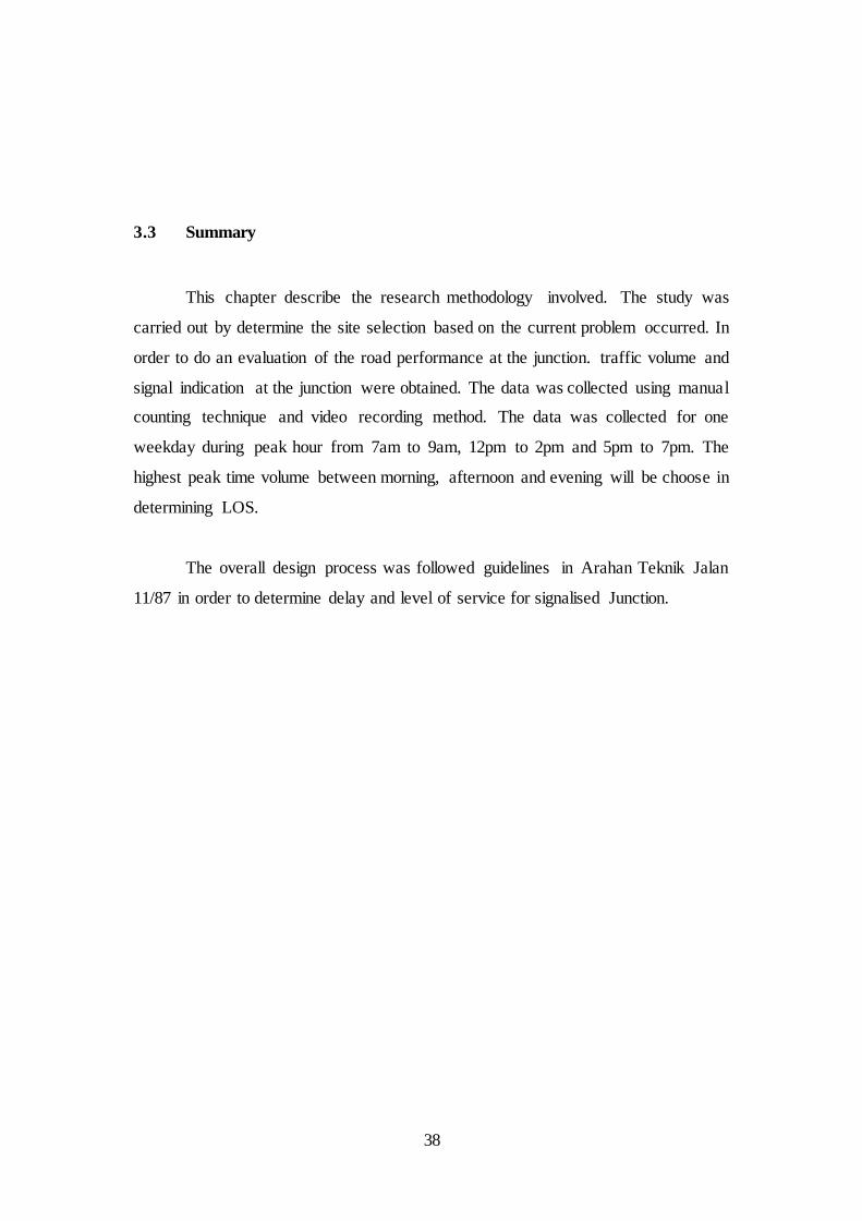
4.2 Vehicle Volume per 15 minutes interval for direction R2 42
4.3 Vehicle Volume per 15 minutes interval for direction R3 43
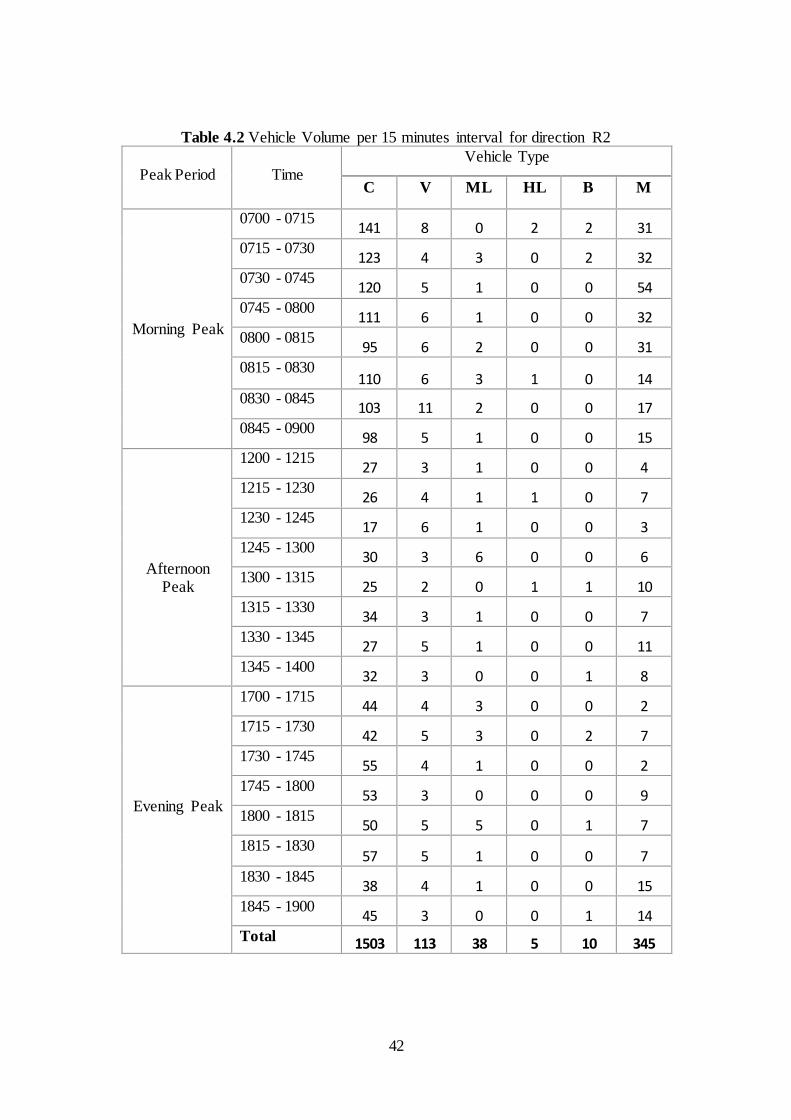
4.4 Vehicle Volume per 15 minutes interval for direction R4 44
4.5 Vehicle Volume per 15 minutes interval for direction R5 45
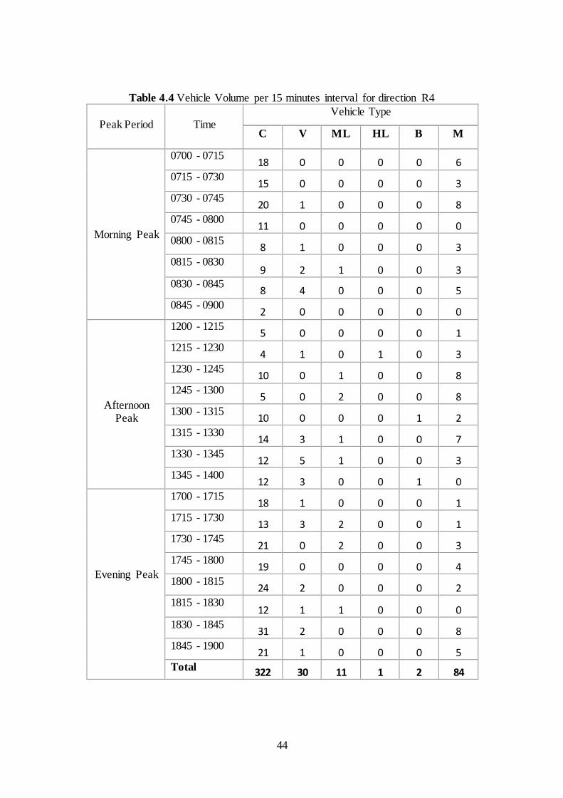
4.6 Vehicle Volume per 15 minutes interval for direction R6 46
4.7 Summary of traffic composition 50
4.8 Summary of current delay calculation 52
4.9 Proposed signal indication 55

x
LIST OF FIGURES
FIGURE NO. TITLE PAGE
2.1 Analysis cases for AWSC junction 9
2.2 Ultrasonic sensor 16
3.1 General Framework 30
3.2 Study Area 33
3.3 Location of video recording 35
3.4 Installation of video record 35
3.5 View from video recording 35
3.6 Direction from six approaches 35
3.7 Excel Form 36
4.1 Junction layout 39
4.2 Traffic Composition in Direction R1 47
4.3 Traffic Composition in Direction R2 48
4.4 Traffic Composition in Direction R3 48
4.5 Traffic Composition in Direction R4 49
4.6 Traffic Composition in Direction R5 49
4.7 Traffic Composition in Direction R6 50
4.8 Traffic Volume in each direction 51
4.9 Time Diagram for current signal indication 52
4.10 Current level of service in each direction 52
4.11 Phase diagram for proposed signal indication 55

xi
LIST OF ABBREVIATIONS
ATJ - Arahan Teknik Jalan
LOS - Level of Service
AWSC - All-Way Stopped Controlled
TWSC - Two Way Stopped Controlled
HCM - Highway Capacity Manual

xii
LIST OF SYMBOLS
d - Delay
S - Saturation flow
λ - Proportion of the cycle that is effectively green for the phase
x - Degree of saturation

xiii
LIST OF APPENDICES
APPENDIX TITLE PAGE
Appendix A Data Collection Table 63


1
CHAPTER 1
INTRODUCTION
1.1 Background of the Study
The analysis of transportation systems is an important research area as it
concerns the daily activities of millions of people moving within a city (Fancello G,
2014). An evaluation of transport network functionally has been widely studied. In
general, the studies quantify road network performance by means of key performance
indicator, that represent the functionality of the network from a specific aspect. Some
investigation focuses on the quality of traffic flow such as the ability to keep traffic
moving as smoothly as possible, using indicators that depend on the geometrical
characteristics: travel time, delay at junction and traffic flow (TRB, 2010).
Junction performance can be measured by determining the volume of vehicles
in certain period, identifying the level of service and the signal indication to figure out
the period of delay at road junction. In the transportation system, traffic light is the
vital component for the effectiveness of the traffic movement. The design of the red,
amber and green time must consider the volume, delay, accident experience and
geometrics. Increase of traffic intensity leads to situations when it becomes impossible
to provide a satisfactory level of traffic servicing with the help of only traffic light
signaling means. Congestion at a section of the road traffic network with traffic signals
is a situation when the average duration of the vehicle delay exceeds the length of the
traffic signalling cycle.
In this case, the queue length can increase, reaching the length of the road
junction. Further development of the road blocking paralyzes larger parts of the road
network and disorganizes the traffic in whole. In certain cases, some of the signal
2
design has led to excessive delay although the volume of vehicles below the traffic
demand. It might lead to drivers behaviour problem such as neglect of signal
indication.
The rapid development in our country has increase the number of vehicles on
the roads that may cause road congestion and will affect the quality of service. In
transportation engineering, the concept of level of service (LOS) is to measure the
qualitative service of roads and illustrates the operational condition of roads and give
impression to the road user.
Highway Capacity Manual (HCM) developed by the transportation research
board of USA provides some procedure to determine level of service. The level of
service have been divided into six classes which is class A to class F. Level A represent
the best performance of traffic where the traffic density will be low, with no
interruption flow speed control by driver desire, low volume, and the drivers can
maintain their desire speed with little or no delay. Level F show the worst quality of
traffic where the demand are exceed the capacity of the road.
Usually, three parameters will be used under this and they are speed and travel
time, delay and density. For this scope of study, LOS was determined by using the
calculation of stopped delay. Many specific delay measures are defined and used as
major of effectiveness in the highway capacity manual.
1.2 Statement of Problem
Road is part of traffic system components. Based on the observation made,
signalised junction at Jalan Pontian Lama-Pulai showed poor performance in term of
traffic movement. Drivers at that area have to wait longer before they were given green
time indication. Rapid development at the area increases the number of populations
3
hence the need to do reassessment of the signalised junction. The design of traffic
signal system may not suitable for the current situation. A few cases of accidents occur
at the junction and it is not safe for the users. This study attempts to evaluate the
junction performance at signalised junction in Jalan Pontian Lama-Pulai.
1.3 Aim and Objective of the Study
The aim of the research is to investigate the signalised junction performance at
Jalan Pontian Lama-Pulai. To achieve the aim, this study is based on the following
objectives:
i. To determine the volume of vehicles at the Jalan Pontian Lama junction
ii. To determine the signal indication at the Jalan Pontian Lama junction
iii. To determine stopped delay at signalised junction
iv. To determine the level of service (LOS)
1.4 Scope of the Study
The scope of the study inclusive the process of determining the performance at
the signalised junction in Jalan Pontian Lama-Pulai. The parameter that was
determined in order to determine road performance are traffic volume, signal
indication, and delay time. The data was collected by using video recording in one
weekdays during peak hour. The obtained data are used to determine stopped delay by
using guidelines in Arahan Teknik Jalan 13/87.


5
CHAPTER 2
LITERATURE REVIEW
2.1 Introduction
The accessibility of the road performance is really important for the human as
everyday we use it to move to another place. The purpose of the road services is to
form a traffic and road transport in a comfort way, secure, excellent movement and
efficient, can be used for multipurpose, can be reach to all land region, development
and stability to drive, to motor, and to support national development with reachable
cost by community. According to Santosa (2005) it is important to make the road
performance evaluation as many factors need to be check such as accessibility
distribution, safety, efficiency, effectivity , reachable cost, and integrity with others
transport system. In order to know the road performance the determination of level of
service of a road network is important as the result will be used to estimate and design
the road network rehabilitation and development. The evaluation has a role in
developing the sustainable transportation system, which has a meaning as a sustainable
system for individual and community.
2.2 Type of Junction Performance
According to Arahan Teknik Jalan 11/87, junction is defined as the general
area where two or more roadways join or cross. It is an integral and important part of
the highway system since much of the efficiency, safety, speed, cost of operation and
maintenance, as well as capacity depend upon its design. There are two type of junction
which are used to design:

6
• Signalised Junction
• Unsignalised Junction
2.2.1 Signalised Junction
The additional element of time allocation is introduced in the signalised
junction for the concept of capacity. A traffic signal essentially allocates time among
conflicting traffic movements that seek to use the same space. Besides, three signal
indications are displayed (red, green and yellow). The red indication may include a
short period during which all indications are red, referred to as an all-red interval,
which with the yellow indications forms the change and clearance interval between
two green phases (HCM, 2000).
2.2.2 Unsignalised Junction
For unsignalised junction, there are three type which is two way stop controlled
(TWSC), all way stop controlled (AWSC), and roundabouts.
2.2.2.1 Characteristic of two way stopped controlled junction
This junction are commonly used in the United States and abroad. To control
the vehicle movements, stop signs were used at such junction. At TWSC junction, the
stop-controlled approaches are referred to as the minor street approaches (public street,

7
private driveways). If the junction are not controlled by stop sign are considered as
major street approaches.
A three-leg junction is considered to be a standard type of TWSC junction if
the single minor street approach such as the stem of the T configuration is controlled
by a stop sign. Three-leg junction where two of the three approaches are controlled
by stop signs are a special form of unsignalised junction control (HCM, 2000).
2.2.2.2 Flow at two way stopped controlled junction
TWSC junction assign the right-of-way among conflicting traffic streams according to
the following hierarcy:
Rank Explanation
1 All conflicting movements yield the right-of-way to any through or
right-turning vehicle on the major street approaches. The major street
through and right-turning movements are the highest-priority
movements at a TWSC junction
2 Vehicles turning left from the major street onto the minor street yield
only to conflicting major street through and right- turning vehicles.
All other conflicting movements at a TWSC junction yield to these
major street left-turning movements. Vehicle turning right from the
minor street onto the major street yield only to conflicting major street
through movements.
3 Minor street through vehicles yield to all conflicting major street
through, right-turning, and left-turning movements.
4 Minor street left-turning vehicles yield to all conflicting major street
through, right-turning, and left turning vehicles and to all conflicting
minor street through and right- turning vehicles.

8
2.2.3 Characteristic of all way stopped controlled junction
This junction needs every vehicle to stop at the junction before continue the
journey. The judgement must be made by each driver whether to proceed into the
junction is a function of traffic conditions on the other approaches. If there is no traffic
present on the other approaches, they can proceed immediately after the stop is made.
If there is traffic on one or more of the other approaches, a driver proceeds only after
determining that there are no vehicles currently in the junction and that it is the driver’s
turn to proceed.
2.2.3.1 Flow at all way stopped controlled junction
Based on the observation that have been made by the previous researchers,
AWSC junction is operating in either two or four-phase depend on the problem occur.
Flow are determined by a consensus of right of way that alternates between the north-
south and east-west streams (for single lane approach) or proceeds in turn to each
junction approach (for a multilane approach junction).
If traffic is present on the subject approach only, vehicles depart as rapidly as
individual drivers can safely accelerate into and clear the junction. This is illustrated
as Case 1 in Figure 2.1

9
Figure 2.1 Analysis cases for AWSC junction
There are the situation where the traffic is present in other approaches that will
increase the saturation headway on the subject approach. In case 2 some uncertainty is
introduced with a vehicle on the opposing approach, and thus the saturation headway
will be greater than for Case 1. In Case 3, vehicles on one of the conflicting approaches
furthest restrict the departure rate of vehicles on the subject approach, and the
saturation headway will be longer than for Cases 1 and 2. In Case 4, two vehicles are
waiting on opposing or conflicting approaches. When all approaches have vehicles as
in case 5, saturation headways are even longer than in the other cases, since the
potential for conflict between vehicles is greatest. The increasing degree of potential
conflict translated directly into both longer driver decision times and saturation
headways. Since no traffic signal control the stream movement or allocates the right -
of-way to each conflicting traffic stream, the rate of departure is controlled by the
interactions between the traffic streams themselves (HCM, 2000).
10
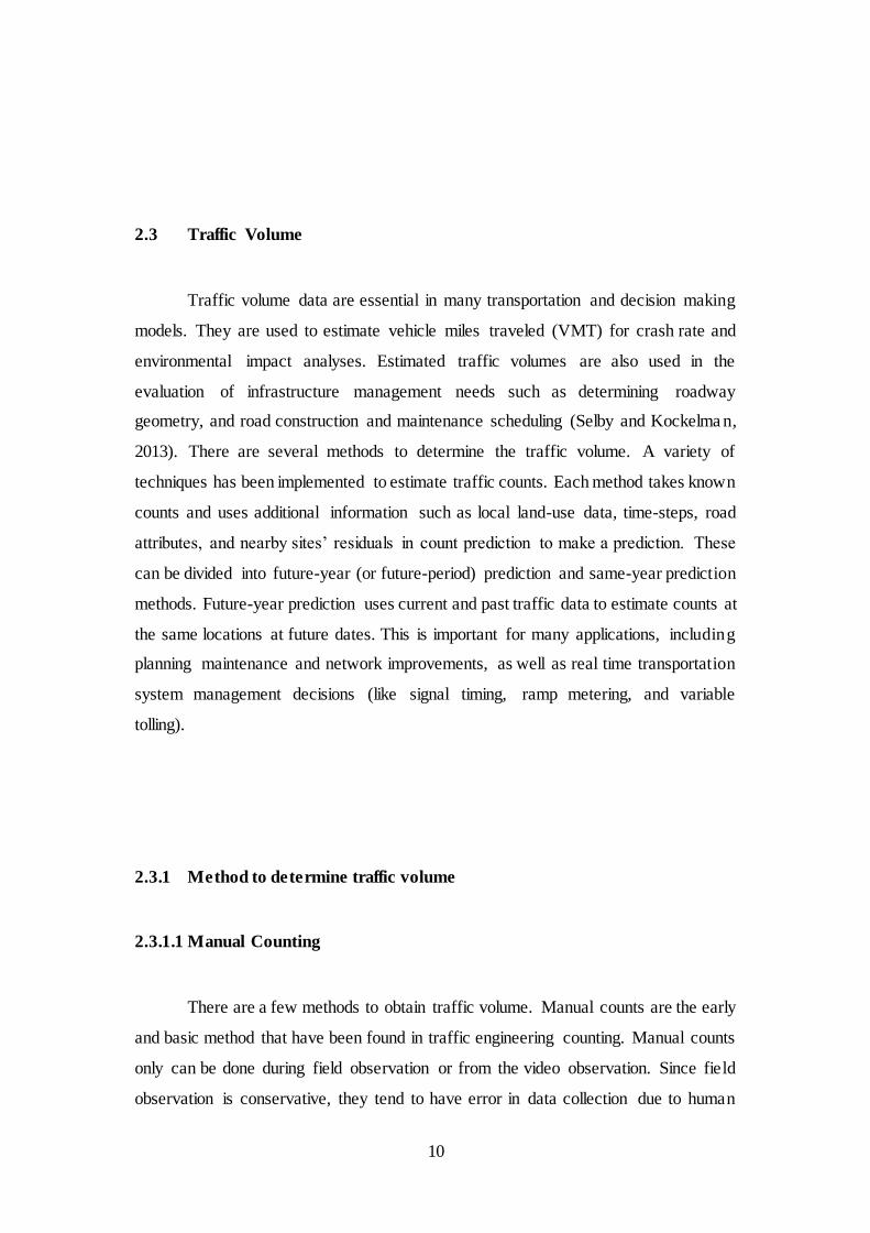
2.3 Traffic Volume
Traffic volume data are essential in many transportation and decision making
models. They are used to estimate vehicle miles traveled (VMT) for crash rate and
environmental impact analyses. Estimated traffic volumes are also used in the
evaluation of infrastructure management needs such as determining roadway
geometry, and road construction and maintenance scheduling (Selby and Kockelma n,
2013). There are several methods to determine the traffic volume. A variety of
techniques has been implemented to estimate traffic counts. Each method takes known
counts and uses additional information such as local land-use data, time-steps, road
attributes, and nearby sites’ residuals in count prediction to make a prediction. These
can be divided into future-year (or future-period) prediction and same-year prediction
methods. Future-year prediction uses current and past traffic data to estimate counts at
the same locations at future dates. This is important for many applications, including
planning maintenance and network improvements, as well as real time transportation
system management decisions (like signal timing, ramp metering, and variable
tolling).
2.3.1 Method to determine traffic volume
2.3.1.1 Manual Counting
There are a few methods to obtain traffic volume. Manual counts are the early
and basic method that have been found in traffic engineering counting. Manual counts
only can be done during field observation or from the video observation. Since field
observation is conservative, they tend to have error in data collection due to human
11
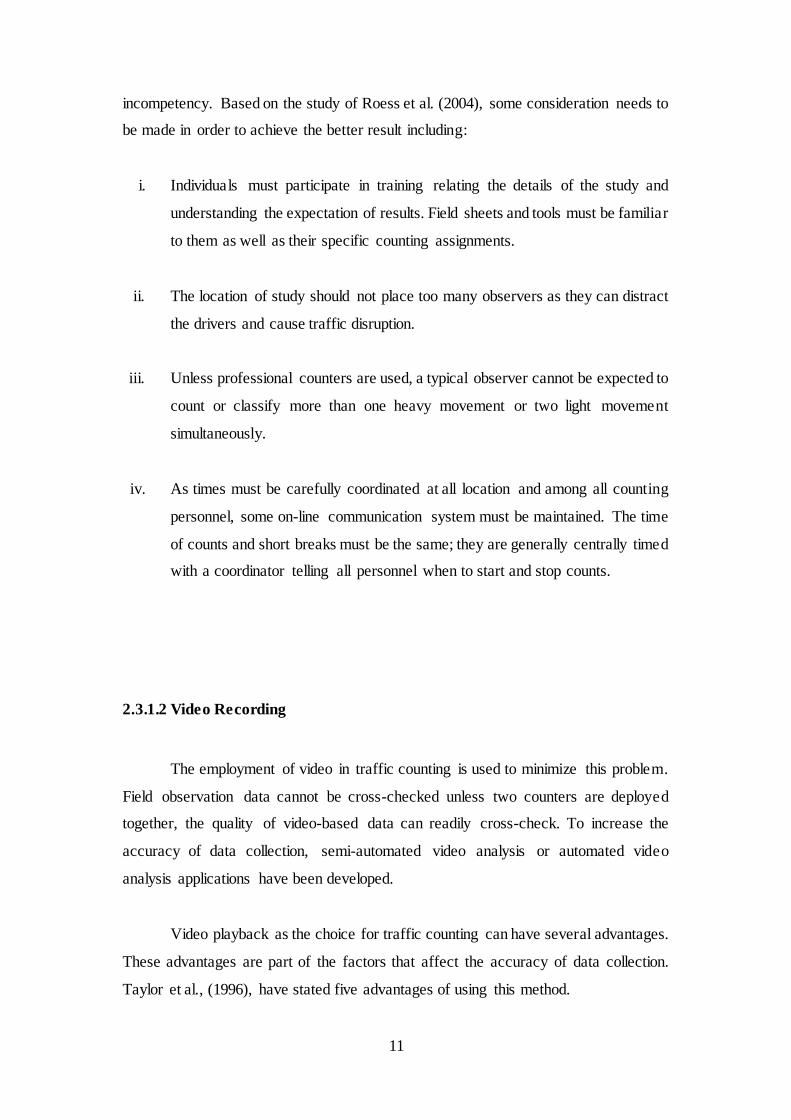
incompetency. Based on the study of Roess et al. (2004), some consideration needs to
be made in order to achieve the better result including:
i. Individuals must participate in training relating the details of the study and
understanding the expectation of results. Field sheets and tools must be familiar
to them as well as their specific counting assignments.
ii. The location of study should not place too many observers as they can distract
the drivers and cause traffic disruption.
iii. Unless professional counters are used, a typical observer cannot be expected to
count or classify more than one heavy movement or two light movement
simultaneously.
iv. As times must be carefully coordinated at all location and among all counting
personnel, some on-line communication system must be maintained. The time
of counts and short breaks must be the same; they are generally centrally timed
with a coordinator telling all personnel when to start and stop counts.
2.3.1.2 Video Recording
The employment of video in traffic counting is used to minimize this problem.
Field observation data cannot be cross-checked unless two counters are deployed
together, the quality of video-based data can readily cross-check. To increase the
accuracy of data collection, semi-automated video analysis or automated video
analysis applications have been developed.
Video playback as the choice for traffic counting can have several advantages.
These advantages are part of the factors that affect the accuracy of data collection.
Taylor et al., (1996), have stated five advantages of using this method.
12
i. Reduced requirement for field staff
ii. Survey is less weather dependent
iii. Existence of permanent record of the scene
iv. Possibility of extracting very detailed data simultaneously or interacting events
as an example vehicle trajectories through a junction, complex turning
movements, junction performance studies, gap acceptance behaviour, traffic
conflicts and
v. Permanent record can be replayed by the analysis if the data contain unusual
or interesting features which require some skill to unravel.
Besides the five advantages of using video playback, the application is
distinguished into three major parts to ensure the accuracy of the count.
First, this application allows the data collectors to count vehicles on a tablet
from pre-recorded videos taken from traffic-monitoring cameras, rather than
deploying to the site where counts are needed. Data collectors can pause, stop, and lay
the videos at their convenience. This functionality is expected to eliminate degraded
performance (for example, missing vehicles) due to fatigue.
Second, the application allows the data collectors’ replay and toggle through
the video to review and correct counts they have already performed.
Third, this application has a reviewer mode, so that a different data collector
can review and correct other users’ cunt can improve the accuracy of the manual count
and minimize human error. This also makes data collectors conscious of the fact that
their counts are under supervision, potentially improving their performance and overall
count accuracy.

13
However, there will be issues of using video cameras. The most notable issue
is the convenient location to set up the video camera unit and battery life. Selection of
a site for the camera will be constrained not only by the requirement for a good view
but also access, security and, if long survey is envisaged, availability of a power supply
(Taylor et al., 1996). The view of the camera must be in a higher place to widen up the
depth of field. Obscuration and parallax will be reduced if a suitable viewpoint is
achieved.
A more accurate ground truth data collection method by using video playback
will give benefit to both transportation researchers and practitioners. The archived
video can be reused for other purposes and will not involve significant capital cost
when video data are available or can be easily collected. By providing accurate data,
long term planning and system performance will get the benefits
2.3.1.3 Automatic Counting Machine
Due to constraints and limitations occur in manual counting, automatic
counting machines are deployed. There are lots of types and each of them have its own
functionality. Taylor et al., (1996), states that different methods predominate in
different countries, partly as reflection of the different ambient conditions (climate,
traffic mix and road conditions) but also as a result of commercial decisions and
historical accident.
The methods explained in Table 2.1 can be separated into two different types
of vehicle detectors. All equipment using pneumatic tube or temporary devices are
portable count techniques while permanent cunts are carried out for 24 hours, all year
round.
14
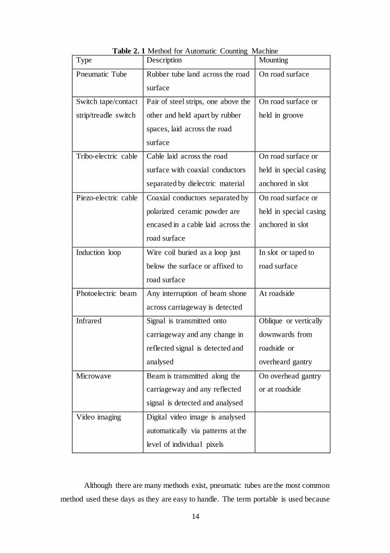
Table 2. 1 Method for Automatic Counting Machine Type Description Mounting
Pneumatic Tube Rubber tube land across the road
surface
On road surface
Switch tape/contact
strip/treadle switch
Pair of steel strips, one above the
other and held apart by rubber
spaces, laid across the road
surface
On road surface or
held in groove
Tribo-electric cable Cable laid across the road
surface with coaxial conductors
separated by dielectric material
On road surface or
held in special casing
anchored in slot
Piezo-electric cable Coaxial conductors separated by
polarized ceramic powder are
encased in a cable laid across the
road surface
On road surface or
held in special casing
anchored in slot
Induction loop Wire coil buried as a loop just
below the surface or affixed to
road surface
In slot or taped to
road surface
Photoelectric beam Any interruption of beam shone
across carriageway is detected
At roadside
Infrared Signal is transmitted onto
carriageway and any change in
reflected signal is detected and
analysed
Oblique or vertically
downwards from
roadside or
overheard gantry
Microwave Beam is transmitted along the
carriageway and any reflected
signal is detected and analysed
On overhead gantry
or at roadside
Video imaging Digital video image is analysed
automatically via patterns at the
level of individual pixels
Although there are many methods exist, pneumatic tubes are the most common
method used these days as they are easy to handle. The term portable is used because
15
it can be transported from location to location to conduct various counts as needed
(Roess et al., 2004).
2.3.1.3.1 Ultrasonic Sensor
Ultrasonic sensors are frequently used as vehicle detection devices because
they are cheaper and more accurate than other types of devices. Most ultrasonic sensors
detect vehicles by measuring from top to bottom or from side to side diagonally
(Jeon.S, 2014). Loop detectors often break as a result of damage from vehicles that
pass over them, and they have high maintenance costs. Loop detectors is installed
beneath the road surface and have been mainly used for the traffic volume
measurement. However, these approaches require that a detector be installed for each
lane because each detector measures only one lane on a road. Furthermore, ultrasonic
sensors require considerable infrastructure on a road. Whenever an ultrasonic sensor
detects the passage of a vehicle on the road, the system measures the distance to the
corresponding vehicle based on its lane location.
Vehicle detection and lane classification can be performed using the data on
the distance to the vehicle and the time required for the vehicle to pass through the
detection range of the ultrasonic sensor. The detection algorithm consists of three parts.
The first part calculates thresholds, which are points at which vehicles are detected in
each lane. The second part filters out unnecessary data, such as noise from the natural
environment. The third part determines the locations of vehicles in multiple lanes and
calculates the traffic volume, based on the filtered data and the calculated thresholds.
The performance of ultrasonic sensors is much better than that of other types of pulse
devices. Ultrasonic detection systems can detect vehicles in multiple zones and
measure their speeds, and they are much cheaper than intrusive systems. Also, they
have disadvantages that its performance is affected by temperature change and air
16
turbulence. However, some modern models, such as those used in our proposed
system, have built-in temperature compensation.
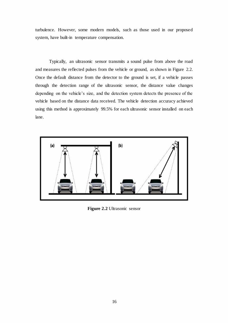
Typically, an ultrasonic sensor transmits a sound pulse from above the road
and measures the reflected pulses from the vehicle or ground, as shown in Figure 2.2.
Once the default distance from the detector to the ground is set, if a vehicle passes
through the detection range of the ultrasonic sensor, the distance value changes
depending on the vehicle’s size, and the detection system detects the presence of the
vehicle based on the distance data received. The vehicle detection accuracy achieved
using this method is approximately 99.5% for each ultrasonic sensor installed on each
lane.
Figure 2.2 Ultrasonic sensor

17
2.4 Traffic Signal
Traffic signals are considered as one of the most effective and important way
of controlling traffic movement at junction. Traffic signals regulate, direct, or warn
motorists and pedestrians to provide their movement through the junction safely and
efficiently. If properly designed, traffic signals can minimise:
• Excessive delay and stop signs and yield signs
• Problems caused by turning movements
• Angle and side collision
• Pedestrian accidents
2.4.1 Components of Traffic Signal Cycle
The time required for one complete sequence of signal indication is called
Cycle time, which is composed of the following components:
• Cycle length: Is the complete sequence of signal indications provided.
• Signal Phase : Is the part of cycle time that includes a green interval,
plus the change and clearance intervals. During each phase a movement
or group of movement given right of way to pass through the junction
safely.
• Interval: Is the part of cycle time that no signal indications change.
• Intergreen: Is the time between the end of a phase and beginning green
indication of another phase. It is composed of Yellow & All red time.
This portion of signal cycle is provided for the vehicles that cannot stop
safely to pass through the junction when green time ends.

18
• All-red: Is the portion of cycle time when signal indications of all the
traffic streams within the junction are Red, Intergreen with all-red
interval called Clearance interval
• Green interval: Is the portion of cycle time that allows a movement or
a group of movements to pass through the junction.
• Red interval: Is the portion of cycle time that a movement or a group
of movements stopped to enter the junction in order to provide
movements pass through the junction safely.
2.4.2 Type of Traffic Signal Operation
Traffic signal controllers are electromechanical or electronic devices that they
regulate the length and sequence of signal indications at junction. Based on the system
of operation traffic signal controllers are classified into:
• Pre-timed controller
• Vehicle-Actuated controller
2.4.2.1 Pre-timed Traffic Controller
In this kind of traffic operation, the cycle length, phase sequence, and timing
of each interval are fixed. Although different timing can be pre-defined over different
times of day but it is still considered as fixed time traffic signal. With the aid of an
internal clock it is possible to allocate at least an AM peak, a PM peak, and an-off peak
signal time. Equation (1) shows the Webster’s optimum cycle time formula, which is
19
derived based on extensive field observation and computer simulation to provide an
excellent procedure for designing traffic signals.
C0 = 1.5𝐿+5
1−𝑌 (1)
Where;
C0 = optimum cycle time to minimise delay (sec)
Y = volume/saturation flow for the critical approach in each phase
L = total lost time/cycle
2.4.2.2 Vehicle-Actuated Traffic Controller
In this kind of traffic operation, the cycle length and phase timings are changing
with the traffic demand by the aid of traffic detectors and required control logic.
Timing of the signals is controlled by traffic demand and in some cases the sequence
of phasing is adjusted too (Roess et al., 2004). They can be divided into:
• Fully actuated: Detectors are installed in every lane of every approach.
Green time is allocated according to the information received from the
detectors and programmed rules.
• Semi-actuated: Detectors are only placed in the lanes of the minor
approach and there are no detectors in the major approach. Major road
signal is always green, except when a call received from one of the
minor approaches.
• Computer control: Computer device is used to control large number of
traffic signals within a network. No computer used for individua l
junction.
20
Although the methodology for implementation actuated traffic signal may vary
according to the type and manufacturer, but they virtually operate based on the same
basic function. For each phase of actuated controller the following features must be set
(Roess et al., 2004)
• Minimum green time, Gmin: It is the smallest amount of green time that
should be allocated to a phase when it is initiated.
• Unit or vehicle extension, U: It is defined as the maximum gap between
actuations of the same detectors, which is added to the minimum green
within the green phase when an actuation received (Figure 2.6).
• Maximum green time, Gmax: It is the maximum length that is allocated
to the green phase in order to limit the amount of green period even if
there is continuous actuation
• Recall switches: These switches are placed on each actuated phase to
arrange the operation of signal when there is no demand.
• Yellow and all-red intervals: This is the same interval provided to pre-
timed controller. They are fixed interval allocated for safe transition
from green to red.
• Pedestrian WALK: This interval must be set for safe crossing of
pedestrians. Since total length of green time is not known in actuated
condition, so the pedestrian WALK interval is set in accordance with
the minimum green time for each phase.
2.4.2.3 Criteria for Justifying Traffic Control Signal
In order to provide traffic signal at the junction, many factors and parameters
must be studied and investigated as it is guided by Manual on Uniform Traffic Control
Devices. After collection of the required data and performing the related analysis, then

21
engineering judgement starts based on the warrants listed and explained by the
MUTCD. Installation of traffic signal is warranted if one or more requirements
specified in any of the warrants are satisfied. These warrants are listed below (Federal
Highway Administration, 2009):
• Warrant 1: Eight hour vehicular volume.
• Warrant 2: Four hour vehicular volume.
• Warrant 3: Peak Hour.
• Warrant 4: Pedestrian volume.
• Warrant 5: School crossing.
• Warrant 6: Coordinated signal system.
• Warrant 7: Crash experience
• Warrant 8: Roadway network.
• Warrant 9: Junction near a grade crossing.
The manual suggests that a group of data must be collected like traffic volume
for each approach, pedestrian volume, speed, and etc, as it is explained clearly in the
manual, in order to evaluate whether or not the junction satisfies the requirements of
one or more or the above warrants.
2.5 Delay
Delay is one of the measure of operational quality or effectiveness of signalised
junctions. It is defined as the amount of tie consumed in traversing the junction, the
difference between the arrival time and the departure time. Delay usually measured in
seconds. The most frequently used forms of delay are defined as follows:

22
• Stopped Time Delay
Stopped time delay is defined as the time a vehicle is stopped in queue while
waiting to pass through the junction, average stopped delay is the average for
all vehicles during a specified time period.
• Approach Delay
Approach delay includes stopped time delay but adds the time loss due to
deceleration from the approach speed to a stop and the time loss due to
reacceleration back to desired speed. Average approach delay is the average
for all vehicles during a specified time period
• Time-in-Queue Delay
Time in queue delay is the total time from a vehicle joining an junction queue
to its discharge across the STOP line on departure. Average time in queue delay
is the average for all vehicles during a specified time period.
• Travel Time Delay
It is the difference between the drivers’ expected travel time through the
junction and actual time taken. This value is rarely used other than the
philosophic concept.
• Control Delay
It is the delay caused by a control device, either a traffic signal or STOP sign.
It is approximately equal to time-in-queue delay plus the acceleration-
deceleration delay component (Roess et al., 2004).
When predicting delay in analytical model, there are three different
components of delay that are needed to be identified.
• Uniform Delay : Is the delay based on the assumption of uniform arrivals and
stable flow with no individual cycle failure

23
• Random Delay : Is additional delay, above and beyond uniform delay, because
flow is randomly distributed rather than uniform at isolated junction.
• Overflow Delay: Is the additional delay that occurs when the capacity of an
individual phase or series of phase is less than the demand or arrival flow rate
2.5.1 Previous Study
There are a lot of method to be used in the past for the delay estimation at the
signalised junction. From the beginning of the traffic engineering growth, the first
technique was suggested by the Bureau of Public Roads’ Committee on Operating
Speeds in Urban Areas, (1955) by calculating the delay manually by using the data
that been taken using photographs of junction approaches. After a few centuries,
Kinzel, (1992) have found a new approaches on estimating delay in the field by
sampling vehicles in queue at a signalised junction. This method can be found in the
Traffic Engineering Handbook (Highway Capacity Manual) which depend on manual
measures of stopped vehicles, slow-moving vehicles, and vehicles passing through the
junction at small time intervals. The control delay was estimated using stop delay and
adjustment factor. This method is very labour intensive, and its accuracy fully depend
on the judgment of user regarding the status of each vehicle and the selection of
adjustment factors.
Quiroga and Bullock, (1999) tried to use Global Positioning System (GPS)
coordinates to estimate control delay. Their method recorded the speed and location of
sampled vehicles every seconds but the method only countered for the small scale of
data as the GPS devices has the limitation on collection of sufficient data. Mousa,
(2002) suggested a method of measuring and analysing control delay by tracking
vehicles’ arrival time at checkpoints manually. In a field experiment, twelve screen

24
lines or checkpoints were marked by one approach with a 27 to a 55m gap between
lines. Crossing times for all vehicles through each screen were manually recorded
using audio cassette recorders. Although it is easy to implement in the field, it is
difficult to apply this method in the multilane situation because the volume of traffic
is high. Therefore, this method also only covers for small range of traffic data.
A study by Abdel-Rahim and Dixon, (2009) produced an automated
measurement of approach delay at signalised junctions. Delay estimation for all
approach and lane groups at the junction was carried out using video detection. This
method only allows the calculation of approach delay, and it was reported to be able
to provide more accurate and less biased delay estimation than those of HCM 2010.
Teply, (1989) suggested a method to measure approach delay in the field using three
timestamps where the arrival time of vehicles to a point located upstream of the
approach, beyond the point that a queue usually could be reach, the timestamp when
the vehicle crosses the stop bar, and the timestamp at the beginning or end of the green
phase of the signal. This method is more acceptable to accurate field implementation
than sampling techniques that require more complex data collection and processing.
However, it cannot measure junction delays, since the turning movements of vehicles
are not tracked as they enter and leave the junction. Another similar study by Kebab
and Dixon, (2007) recommended installing additional detectors to cover all the lanes
separately. In this way, the approach delay for different lane groups can be obtained.
As the study did not identify vehicle turning movements, this technique cannot be used
to measure junction control delay. In a recent study by Forbush, (2011) developed an
automated method to estimate traffic delay at junction in real time. However, the delay
estimation focused on through lanes only, and situations where lanes are shared were
not considered in this study. A study by Shatnawi, (2018) found a new method to
calculate automatically the approach delay and intersection delay at a signalised
junction by using the Automated Vehicle Delay Estimation Technique (AVDET). It
was found to perform very effectively under different traffic scenarios.
25
2.6 Level of Service
Level of service defined as the quality measure as describes the operational
condition of a traffic facility serving traffic streams. The quality of service of the traffic
facility is described in term of service measures such as speed and travel time, freedom
to manoeuvre, interruption in traffic, and comfort and convenience. For signalised
junction, many types of approach are used to determine level of service for a junction
with different parameter such as Highway Capacity Manual 2000 (American
Approach) and Arahan Teknik Jalan 11/87 (Malaysian Approach).
2.6.1 American Approach
According to Highway Capacity Manual, (2000), there are six levels of service
that is defined by Highway Capacity Manual for each type of facility as they shown in
Table 2.2. Each level of service describes a range of operating condition and the
driver’s perception to those conditions. Safety is not one of the measures that are
included in establishing service levels. Level of service of a signalised junction is
evaluated on the basis of control delay per vehicle (sec/veh).
The average control delay per vehicle for a typical 15-minute analysis period
is used to indicate LOS criteria of signalised junction.

26
Table 2.2 LOS criteria for junction
LOS (a) Control Delay per Vehicle (s/veh)
A ≤ 10
B >10-20
C >20-35
D >35-55
E >56-80
F >80
Source: HCM2000 16-2
LOS A: Very short delay and most vehicles do not stop as result of favourable
progressions, arrival of most vehicles during green phase, and short cycle length
LOS B: Short delay and many vehicles do not stop or stop for short time as a result of
short lengths and good progression
LOS C: Moderate delay, many vehicles have to stop and occasional individual cycle
failures as a result of some combination of long cycle lengths, high volume to capacity
ratios, and unfavourable progression.
LOS D: Longer delays, many vehicles have to stop and a noticeable number of
individual cycle failures as a result of some combination of long cycle lengths, high
volume to capacity ratios, and unfavourable progression
LOS E: Long delays and frequent individual cycle failures result from one or both of
the following long cycle lengths or high volume to capacity ratios, which, in turn,
result in poor progression
LOS F: Delays considered unacceptable to most drivers occur when the vehicle arrival
rate is greater than the capacity of the junction for extended period of time

27
2.6.2 Malaysian Approach
Based on Arahan Teknik Jalan 11/87, the LOS criteria is associated with the
delay values for signalised junction as shown in Table 2.3. The traffic forecast for any
junction design shall be at least the Level of Service ‘D’ maintained throughout the
forecasted year (10 years) as be mentioned in ATJ 11/87 in Table 2.4 for rural road. If
such level of service cannot be sustained throughout the design life of the projected
forecast then the designer has to propose mitigation measures.
Table 2.3 LOS criteria for signalised junction
Table 2.4 Minimum requirement LOS for Malaysian Road
AREAS CATEGORY OF ROAD LEVEL OF
SERVICE
RURAL Expressway
Highway
Primary
Secondary
Minor
C
C
D
D
E
URBAN Expressway
Arterial
Collector
Local Street
C
D
D
E
28
2.7 Summary
Junction performance is an important measure as it is part of traffic system
components. The junction performance must accomplish with the objective given. The
parameter is needed to measure the performance of signalised junction is traffic
volume, signal indication, and delay. Video recording technique was used for this
scope of study. Level of service is qualitative parameter described the actual traffic
operation condition at the junction and used to access the performance of the junction.
Arahan Teknik Jalan 11/87 use to estimate delay at the junction based on the parameter
needed.
29
CHAPTER 3
RESEARCH METHODOLOGY
3.1 Introduction
This chapter describes the method to carry out the study. The main objective
of the study is to evaluate the performance at signalised junction by determining the
level of service of the road. The study was started with identifying the problem, which
is expressed as problem statement. The second step was setting the objectives of the
study. Then, based on the targeted objectives, literature of the study was collected from
different resources and reviewed. In this chapter, the rest of the steps required for
conducting this study are going to be explained.
3.2 General Framework
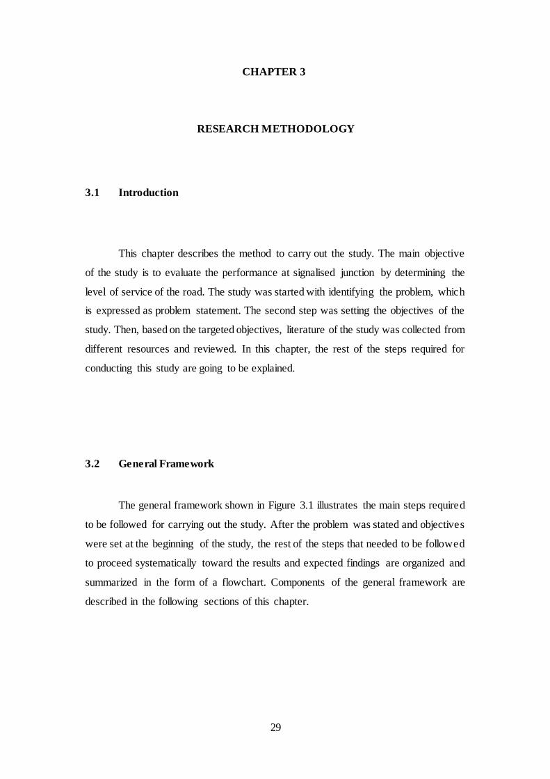
The general framework shown in Figure 3.1 illustrates the main steps required
to be followed for carrying out the study. After the problem was stated and objectives
were set at the beginning of the study, the rest of the steps that needed to be followed
to proceed systematically toward the results and expected findings are organized and
summarized in the form of a flowchart. Components of the general framework are
described in the following sections of this chapter.
30
Figure 3.1: General Framework

31
3.2.1 Identification of the Required Data
Before starting any study, a set of parameters and required data should be
identified in order to carry out the analysis systematically without any missing
variables and re-doing the data collection. To avoid interruption in the analysis stage,
the following sets of parameters were defined.
3.2.1.1 Identification of the Required Data
This included all the existing and required information about the layout of the
junction such as; junction of approaches, number of lanes, lane widths, and median.
These data were collected by measurements achieved in field.
3.2.1.2 Traffic Data
The traffic data included all the necessary information about the characteristics
of the traffic stream using the facility. They were classified into:
• Traffic volume: Number of vehicles crossing the stop line of each approach in
unit of time (usually every 15 minutes)
• Turning proportion: Identifying the number of vehicles turning to different
directions of the junction for each approach
• Traffic composition: Traffic stream are not composed of identical vehicles, and
each type of vehicle has a different impact on the traffic characteristics of the
facilities. Therefore, traffic volume was classified into different vehicle groups
according to the Malaysian HCM 2006

32
3.2.1.3 Traffic Signal Indication
This included all the information about the traffic signal provided at the
junction such as; cycle time, phase splits, green time and clearance interval (Yellow+
All-red) for each phase. The traffic signal data was collected simultaneously with the
other traffic data mentioned earlier.
3.2.2 Data Collection Instruments and Technique
The following instruments were used in the data collection process to facilities
obtaining the required data defined previously.
• Stop-watch: to measure the cycle length, green time, yellow+ all-red interval
• Video camera: to record traffic movements at the junction, from which traffic
volume, turning proportions, traffic composition, and signal timing
• Excel form: transfer data from video camera into traffic composition (shown
in Appendix A).
3.2.3 Site Selection
Before starting any field measurements and data collection for conducting a
study, if the site is not a specific place then several sites has to be visited and

33
investigated in order to select the must proper one based on the suitability of the
geometry of the site to achieve video recording and other in-situ measurements. After
examining several junction, Jalan Pontian Lama-Pulai junction selected as the case
study (Figure 3.2).
Jalan Pontian Lama is a road connecting Jalan Pulai in Skudai-Taman
Universiti. Skudai is town located at the South-West of Johor Bahru state at South of
Malaysia. The junction of Jalan Pontian Lama and Jalan Pulai is a signalised junction
with fixed-time traffic signal system. Each approaches of the junction composed of
two lanes both ways. Each approach is provided with individual signal phase, which
means the cycle time is divided into three signal phases. The area is residential.
Figure 3.2 Study Area
34
3.2.4 Data Collection
In order to do an evaluation of the performance at the junction. traffic volume
and signal indication at the junction were obtained. The data was collected using
manual counting technique and video recording method. Video recording was installed
by attaching it at lamp post. It was installed 3 metres from the bottom of lamp post in
order to get good overview of the site. The data was collected for one weekday during
peak hour from 7am to 9am, 12pm to 2pm and 5pm to 7pm. Figure 3.3 and Figure 3.4
shows the location of video recording while Figure 3.5 shows an overview of site from
video. Figure 3.6 shows the direction of traffic volume for all six approaches. Based
on the collection of data made for 3 peak time, only the highest peak time volume will
be used to evaluate the current signalised junction performance.

35
Figure 3.3: Location of video recording
Figure 3.4: Installation of video record
Figure 3.5: View from video recording
Figure 3.6: Direction from six approaches
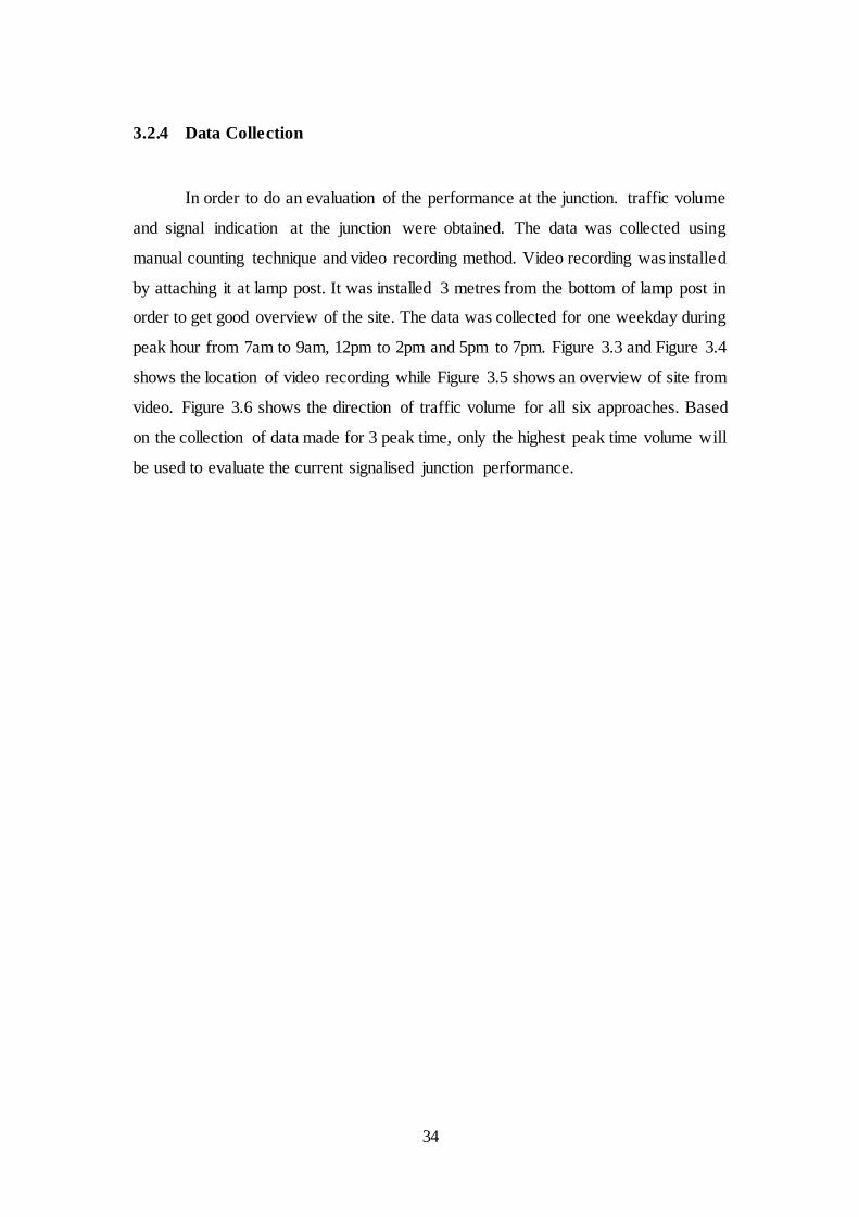
3.2.5 Data Extraction
Field-measured data were extracted and summarized into the required usable
forms. Data from the video records were extracted by using conventional video player
and then were keyed in into excel form as shown in Figure 3.7. Traffic data volume
36
will be converted into pcu/hr to obtain total traffic composition for each direction as
the data will be used as an input in calculation of stopped delay.
Figure 3.7: Excel Form
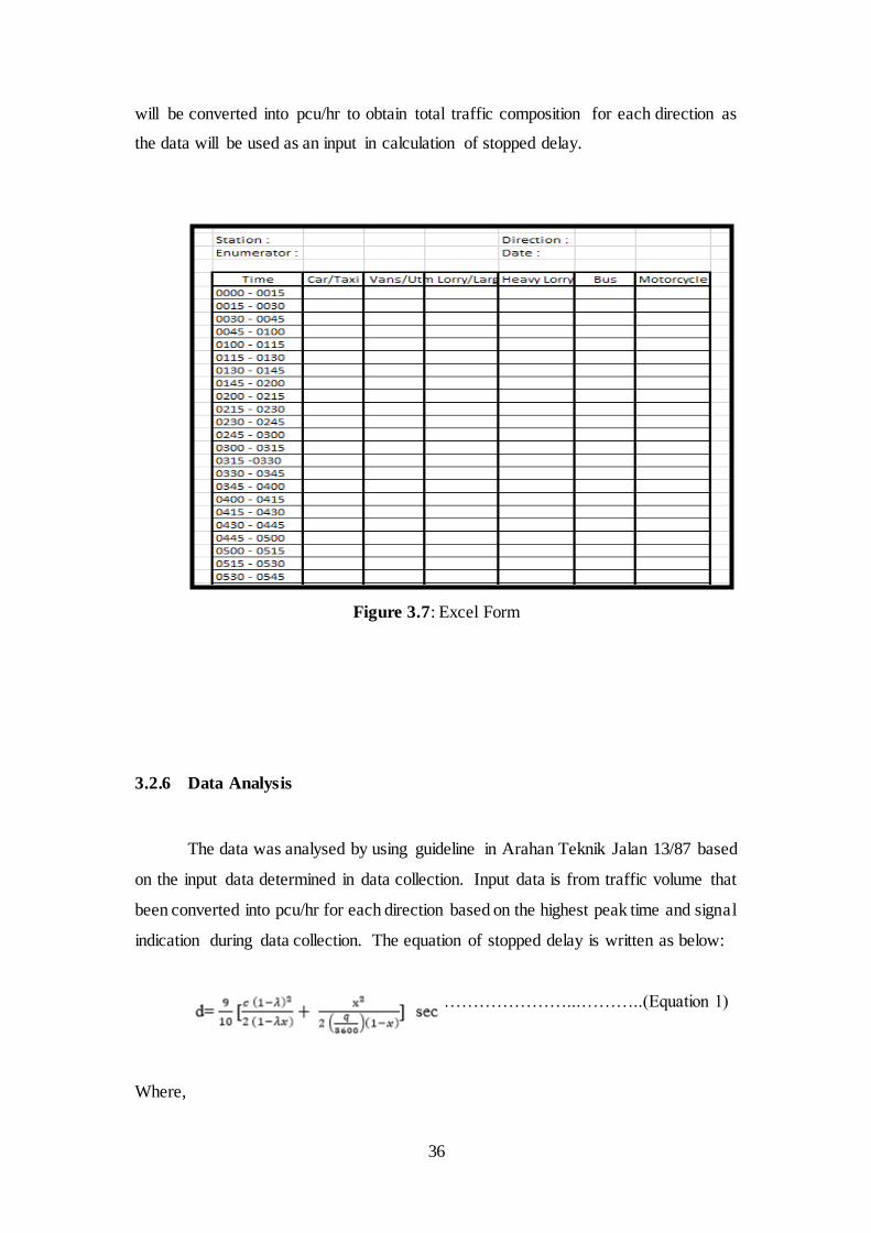
3.2.6 Data Analysis
The data was analysed by using guideline in Arahan Teknik Jalan 13/87 based
on the input data determined in data collection. Input data is from traffic volume that
been converted into pcu/hr for each direction based on the highest peak time and signal
indication during data collection. The equation of stopped delay is written as below:
………………………..………………………………...………..(Equation 1)
Where,

37
q= traffic volume, pcu/sec
S= saturation flow , pcu/sec
λ= proportion of the cycle that is effectively green for the phase , g/c
x= degree of saturation , q/λS
From the stopped delay obtained from the Equation 1, the level of service for
each direction can be determined by referring to Table 3.1 which has been discussed
in Chapter 2.
Table 3.1: Level of Service
3.2.7 Result and Discussion
The final step of the operation analysis process was interpreting the results. If
the result does not meet the requirement according to ATJ 11/87 which indicate that
minimum level of service at the junction is ‘D’ as be mentioned in ATJ 11/87 (A Guide
to the Design of at Grade-Intersections), the junction needs to be redesign the traffic
signal cycle.
38
3.3 Summary
This chapter describe the research methodology involved. The study was
carried out by determine the site selection based on the current problem occurred. In
order to do an evaluation of the road performance at the junction. traffic volume and
signal indication at the junction were obtained. The data was collected using manual
counting technique and video recording method. The data was collected for one
weekday during peak hour from 7am to 9am, 12pm to 2pm and 5pm to 7pm. The
highest peak time volume between morning, afternoon and evening will be choose in
determining LOS.
The overall design process was followed guidelines in Arahan Teknik Jalan
11/87 in order to determine delay and level of service for signalised Junction.

39
CHAPTER 4
RESULT AND ANALYSIS
4.1 Introduction
The aim of the study is to evaluate the road performance of a signalised
junction. In this chapter detailed analysis of the evaluation process is presented. The
analysis process starts from traffic volume studies, signal indication measurement,
stopped delay measurements, and level of service.
4.2 Traffic Volume
The site consists of T-junction with North, South and East direction. Each
approach is composed of four lanes (two lane each direction). Each lane is 4.4m wide.
East approach has 0.5m wide built out median. While at the apposing approach both
sides are separated by painting. Figure 4.1 shows the layout of the junction.
Figure 4.1 Junction layout

40
Video recording technique was used for traffic volume studies of Jalan Pontian
Lama-Pulai junction. Table 4.1 to Table 4.6 shows the summary of traffic volume for
all 8 direction of the junction respectively. The study was conducted for 2 hours for
every peak hours in a day. From 7am to 9am, 12pm to 2pm and 5pm to 7pm. The total
number of observed vehicles during the study time was 6487 vehicles. From previous
Chapter 3 in data collection has been highlighted that the highest peak time volume
between morning peak, afternoon peak and evening peak will be choose to determine
current performance in signalised junction. From data extraction, it is found that
average morning peak volume is highest among others peak time. Therefore, evening
peak time volume is chosen for calculation.

41
Table 4.1 Vehicle Volume per 15 minutes interval for direction R1
Peak Period
Time
Vehicle Type
C V ML HL B M
Morning Peak
0700 - 0715 55 16 3 0 2 16
0715 - 0730 35 4 0 0 0 17
0730 - 0745 50 6 1 0 0 15
0745 - 0800 41 3 6 0 0 11
0800 - 0815 37 8 0 0 1 15
0815 - 0830 34 3 1 0 0 7
0830 - 0845 40 5 1 0 0 11
0845 - 0900 32 3 0 0 1 14
Afternoon
Peak
1200 - 1215 23 3 6 0 1 5
1215 - 1230 33 2 9 1 0 8
1230 - 1245 40 6 1 0 0 15
1245 - 1300 38 3 6 0 0 11
1300 - 1315 37 2 7 0 1 15
1315 - 1330 34 3 1 0 0 7
1330 - 1345 28 1 1 0 0 11
1345 - 1400 32 3 0 0 1 14
Evening Peak
1700 - 1715 54 3 2 0 0 19
1715 - 1730 50 8 4 0 0 21
1730 - 1745 64 10 5 0 1 29
1745 - 1800 58 5 7 0 0 25
1800 - 1815 60 4 7 0 0 9
1815 - 1830 70 11 5 0 0 14
1830 - 1845 50 10 6 0 0 10
1845 - 1900 65 6 6 0 0 15
Total 1060 128 85 1 8 334
42
Table 4.2 Vehicle Volume per 15 minutes interval for direction R2
Peak Period
Time
Vehicle Type
C V ML HL B M
Morning Peak
0700 - 0715 141 8 0 2 2 31
0715 - 0730 123 4 3 0 2 32
0730 - 0745 120 5 1 0 0 54
0745 - 0800 111 6 1 0 0 32
0800 - 0815 95 6 2 0 0 31
0815 - 0830 110 6 3 1 0 14
0830 - 0845 103 11 2 0 0 17
0845 - 0900 98 5 1 0 0 15
Afternoon
Peak
1200 - 1215 27 3 1 0 0 4
1215 - 1230 26 4 1 1 0 7
1230 - 1245 17 6 1 0 0 3
1245 - 1300 30 3 6 0 0 6
1300 - 1315 25 2 0 1 1 10
1315 - 1330 34 3 1 0 0 7
1330 - 1345 27 5 1 0 0 11
1345 - 1400 32 3 0 0 1 8
Evening Peak
1700 - 1715 44 4 3 0 0 2
1715 - 1730 42 5 3 0 2 7
1730 - 1745 55 4 1 0 0 2
1745 - 1800 53 3 0 0 0 9
1800 - 1815 50 5 5 0 1 7
1815 - 1830 57 5 1 0 0 7
1830 - 1845 38 4 1 0 0 15
1845 - 1900 45 3 0 0 1 14
Total 1503 113 38 5 10 345

43
Table 4.3 Vehicle Volume per 15 minutes interval for direction R3
Peak Period
Time
Vehicle Type
C V ML HL B M
Morning Peak
0700 - 0715 27 5 1 0 1 3
0715 - 0730 19 0 1 0 0 1
0730 - 0745 29 1 0 0 0 3
0745 - 0800 20 2 0 0 0 4
0800 - 0815 11 4 0 1 0 0
0815 - 0830 17 0 1 0 0 0
0830 - 0845 15 2 0 0 0 0
0845 - 0900 10 0 0 0 0 3
Afternoon
Peak
1200 - 1215 10 1 1 0 0 4
1215 - 1230 23 5 2 1 0 2
1230 - 1245 15 6 1 0 0 4
1245 - 1300 26 3 6 0 0 6
1300 - 1315 12 3 0 0 1 6
1315 - 1330 23 3 1 0 0 7
1330 - 1345 18 5 1 0 0 11
1345 - 1400 7 3 0 0 1 14
Evening Peak
1700 - 1715 19 1 0 0 0 3
1715 - 1730 13 2 0 0 0 0
1730 - 1745 13 5 1 0 0 5
1745 - 1800 17 3 0 0 0 0
1800 - 1815 9 0 0 0 0 3
1815 - 1830 10 3 0 0 0 2
1830 - 1845 8 1 0 0 0 1
1845 - 1900 11 1 0 0 0 0
Total 382 59 16 2 3 82
44
Table 4.4 Vehicle Volume per 15 minutes interval for direction R4
Peak Period
Time
Vehicle Type
C V ML HL B M
Morning Peak
0700 - 0715 18 0 0 0 0 6
0715 - 0730 15 0 0 0 0 3
0730 - 0745 20 1 0 0 0 8
0745 - 0800 11 0 0 0 0 0
0800 - 0815 8 1 0 0 0 3
0815 - 0830 9 2 1 0 0 3
0830 - 0845 8 4 0 0 0 5
0845 - 0900 2 0 0 0 0 0
Afternoon
Peak
1200 - 1215 5 0 0 0 0 1
1215 - 1230 4 1 0 1 0 3
1230 - 1245 10 0 1 0 0 8
1245 - 1300 5 0 2 0 0 8
1300 - 1315 10 0 0 0 1 2
1315 - 1330 14 3 1 0 0 7
1330 - 1345 12 5 1 0 0 3
1345 - 1400 12 3 0 0 1 0
Evening Peak
1700 - 1715 18 1 0 0 0 1
1715 - 1730 13 3 2 0 0 1
1730 - 1745 21 0 2 0 0 3
1745 - 1800 19 0 0 0 0 4
1800 - 1815 24 2 0 0 0 2
1815 - 1830 12 1 1 0 0 0
1830 - 1845 31 2 0 0 0 8
1845 - 1900 21 1 0 0 0 5
Total 322 30 11 1 2 84

45
Table 4.5 Vehicle Volume per 15 minutes interval for direction R5
Peak Period
Time
Vehicle Type
C V ML HL B M
Morning Peak
0700 - 0715 7 2 0 0 0 5
0715 - 0730 7 1 0 0 0 1
0730 - 0745 8 1 0 0 0 2
0745 - 0800 9 2 0 0 0 1
0800 - 0815 17 0 0 0 0 4
0815 - 0830 23 2 0 0 0 4
0830 - 0845 18 0 0 0 0 6
0845 - 0900 9 1 1 0 0 6
Afternoon
Peak
1200 - 1215 7 4 3 0 2 4
1215 - 1230 11 2 1 0 1 1
1230 - 1245 10 4 1 0 0 4
1245 - 1300 8 3 6 0 0 5
1300 - 1315 13 6 0 0 1 5
1315 - 1330 10 3 1 0 0 7
1330 - 1345 7 5 1 0 0 10
1345 - 1400 11 3 0 0 1 2
Evening Peak
1700 - 1715 19 4 0 0 0 3
1715 - 1730 29 5 1 0 0 2
1730 - 1745 32 2 1 0 0 8
1745 - 1800 23 4 2 0 0 4
1800 - 1815 28 0 0 0 0 3
1815 - 1830 30 4 0 0 0 5
1830 - 1845 25 1 1 0 0 4
1845 - 1900 18 1 0 0 0 4
Total 379 60 19 0 5 100
46
Table 4.6 Vehicle Volume per 15 minutes interval for direction R6
Peak Period
Time
Vehicle Type
C V ML HL B M
Morning Peak
0700 - 0715 40 4 1 0 0 7
0715 - 0730 20 0 0 0 0 4
0730 - 0745 31 3 0 0 0 6
0745 - 0800 23 8 0 0 0 3
0800 - 0815 30 1 1 0 1 7
0815 - 0830 25 3 0 0 1 3
0830 - 0845 35 1 1 0 0 1
0845 - 0900 25 6 0 0 0 7
Afternoon
Peak
1200 - 1215 13 0 0 1 0 5
1215 - 1230 26 0 1 0 0 1
1230 - 1245 17 4 1 0 0 8
1245 - 1300 23 3 2 0 0 11
1300 - 1315 14 1 0 0 1 12
1315 - 1330 19 1 1 0 0 7
1330 - 1345 24 1 1 0 0 10
1345 - 1400 10 3 0 0 1 8
Evening Peak
1700 - 1715 50 3 2 0 0 16
1715 - 1730 44 2 3 0 0 10
1730 - 1745 82 7 1 0 0 15
1745 - 1800 98 1 0 0 0 9
1800 - 1815 88 7 3 0 0 18
1815 - 1830 73 2 0 0 0 19
1830 - 1845 80 8 0 0 0 15
1845 - 1900 95 3 2 0 0 17
Total 985 72 20 1 4 219
47
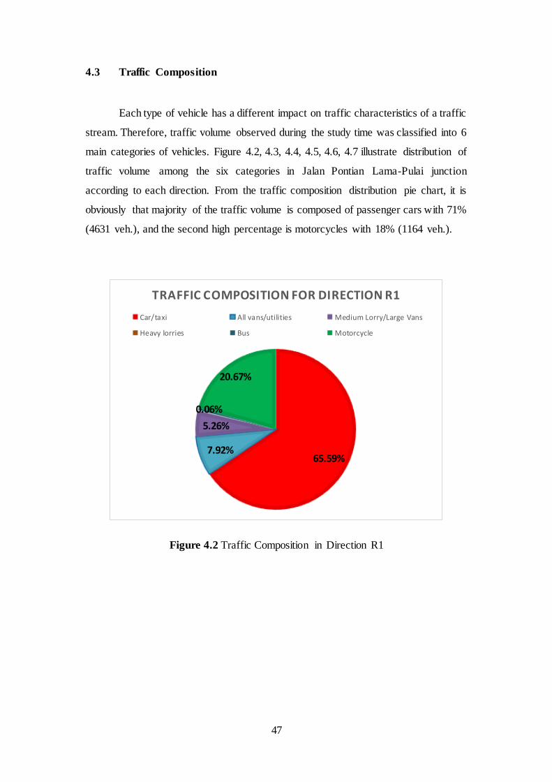
4.3 Traffic Composition
Each type of vehicle has a different impact on traffic characteristics of a traffic
stream. Therefore, traffic volume observed during the study time was classified into 6
main categories of vehicles. Figure 4.2, 4.3, 4.4, 4.5, 4.6, 4.7 illustrate distribution of
traffic volume among the six categories in Jalan Pontian Lama-Pulai junction
according to each direction. From the traffic composition distribution pie chart, it is
obviously that majority of the traffic volume is composed of passenger cars with 71%
(4631 veh.), and the second high percentage is motorcycles with 18% (1164 veh.).
Figure 4.2 Traffic Composition in Direction R1
65.59%7.92%
5.26%
0.06%
20.67%
TRAFFIC COMPOSITION FOR DIRECTION R1
Car/taxi All vans/utilities Medium Lorry/Large Vans
Heavy lorries Bus Motorcycle

48
Figure 4.3 Traffic Composition in Direction R2
Figure 4.4 Traffic Composition in Direction R3
74.63%
5.61%1.89%
0.25%
0.50%17.13%
TRAFFIC COMPOSITION FOR DIRECTION R2
Car/taxi All vans/utilities Medium Lorry/Large Vans
Heavy lorries Bus Motorcycle
70.22%
10.85%
2.94%
0.37%
0.55%15.07%
TRAFFIC COMPOSITION FOR DIRECTION R3
Car/taxi All vans/utilities Medium Lorry/Large Vans
Heavy lorries Bus Motorcycle
49
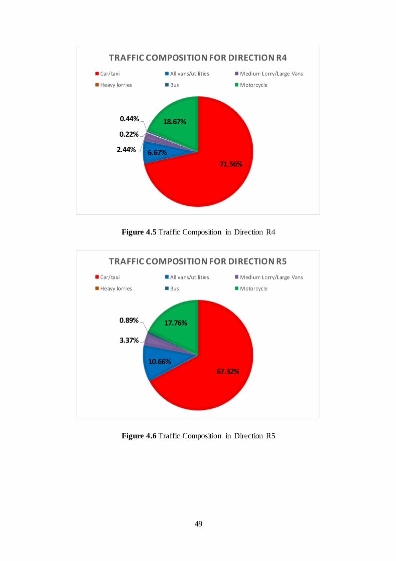
Figure 4.5 Traffic Composition in Direction R4
Figure 4.6 Traffic Composition in Direction R5
71.56%
6.67%2.44%
0.22%
0.44% 18.67%
TRAFFIC COMPOSITION FOR DIRECTION R4
Car/taxi All vans/utilities Medium Lorry/Large Vans
Heavy lorries Bus Motorcycle
67.32%10.66%
3.37%
0.89% 17.76%
TRAFFIC COMPOSITION FOR DIRECTION R5
Car/taxi All vans/utilities Medium Lorry/Large Vans
Heavy lorries Bus Motorcycle
50
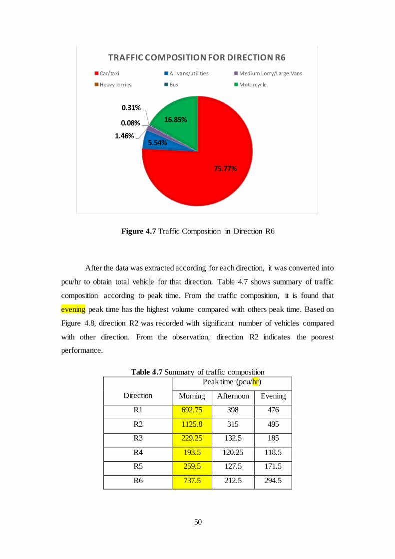
Figure 4.7 Traffic Composition in Direction R6
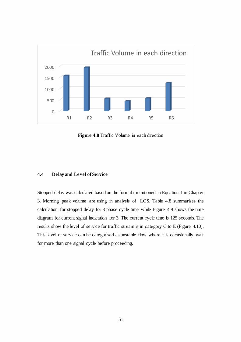
After the data was extracted according for each direction, it was converted into
pcu/hr to obtain total vehicle for that direction. Table 4.7 shows summary of traffic
composition according to peak time. From the traffic composition, it is found that
evening peak time has the highest volume compared with others peak time. Based on
Figure 4.8, direction R2 was recorded with significant number of vehicles compared
with other direction. From the observation, direction R2 indicates the poorest
performance.
Table 4.7 Summary of traffic composition
Direction
Peak time (pcu/hr)
Morning Afternoon Evening
R1 692.75 398 476
R2 1125.8 315 495
R3 229.25 132.5 185
R4 193.5 120.25 118.5
R5 259.5 127.5 171.5
R6 737.5 212.5 294.5
75.77%
5.54%1.46%
0.08%
0.31%
16.85%
TRAFFIC COMPOSITION FOR DIRECTION R6
Car/taxi All vans/utilities Medium Lorry/Large Vans
Heavy lorries Bus Motorcycle
51
Figure 4.8 Traffic Volume in each direction
4.4 Delay and Level of Service
Stopped delay was calculated based on the formula mentioned in Equation 1 in Chapter
3. Morning peak volume are using in analysis of LOS. Table 4.8 summarises the
calculation for stopped delay for 3 phase cycle time while Figure 4.9 shows the time
diagram for current signal indication for 3. The current cycle time is 125 seconds. The
results show the level of service for traffic stream is in category C to E (Figure 4.10).
This level of service can be categorised as unstable flow where it is occasionally wait
for more than one signal cycle before proceeding.
0
500
1000
1500
2000
R1 R2 R3 R4 R5 R6
Traffic Volume in each direction

52
Figure 4.9 Time Diagram for current signal indication
Table 4.8 Summary of current delay calculation
From North South East
To East (R?) South North East North
q 738 260 229 194 1126
S 4725 4620 4620 4725 4620
g 45 45 36 36 36
c 125 125 125 125 125
λ 0.3600 0.3600 0.2880 0.2880 0.2880
x 0.434 0.156 0.172 0.143 0.846
d(sec) 28.0 24.6 33.2 29.9 44.8
LOS D C D D E
Figure 4.10 Current level of service in each direction
C

53
In previous Chapter 2, the minimum required level of service for the signalised
junction based on ATJ 11/87 is in category D. If such level of service cannot be
sustained throughout the design life of the projected forecast then the designer has to
propose mitigation measure. Current level of service in studied area was not fulfill the
minimum criteria since level of service in direction R2 have the poorest performance
(LOS E). Therefore, we need to redesign signal indication for the junction.
To accommodate junction demand, the traffic signal indication was redesigned
by referring to ATJ 13/87. The new cycle time is 90 seconds which is shorter compared
to the current cycle time. A few directions show some improvement in term of level
of service as shown in Table 4.9 yet some remains the same while Figure 4.11 shows
phase diagram for proposed signal indication.
Phase 1 2 3
From North South East
To East South North East North
q (pcu/h) 738 260 229 194 1126
S' (pcu/h) 4725 4620 4620 4725 4620
y = q/S' 0.156 0.056 0.050 0.041 0.244
Ymax 0.156 0.05 0.244
sum Y= 0.45
b) assumptions
All red period,R = 2sec Amber, a = 3sec
Lost time due to late start,l = 3sec
Intergeen period, l = a+R
= 5sec
Total lost time per cycle,L = (l-a)1 + (l-a)2 + (l-a)3 + l1 +l2 +l3
= 12 sec

54
Optimum cycle time, C0 = (1.5L + 5)/(1-Y)
= 42 sec
0.75C0<C<1.5C0
Therefore, choose C0 = 60 sec
c) effective green time
gn= yn(C0-L)/Y
g1 = 10 sec
g2 = 5 sec
g3 = 26 sec
d) actual green time
Gn=gn + l + R
G1 = 15 sec
G2 = 10 sec
G3 = 60 sec
e) display green time
Kn= Gn-a-R
K1 = 10 sec
K2 = 5 sec
K3 = 26 sec

55
Table 4.9 Proposed signal indication
From North South East
To East South North East North
q 738 260 229 194 1126
S 4725 4620 4620 4725 4620
g 10 10 5 5 26
c 60 60 60 60 60
λ 0.1667 0.1667 0.0833 0.0833 0.4333
x 0.937 0.338 0.595 0.493 0.562
d(sec) 24.9 20.9 30.1 27.7 12.5
LOS C C D D B
Figure 4.11 Phase diagram for proposed signal indication
56
4.5 Summary
Based on the result presented in this chapter, the following conclusion can be
drawn:
i. Traffic volume at the junction for 6 hours observation was 6487 vehicles. It
was found that the highest traffic composition is passengers car and the second
highest is motorcycles. Based on the six direction, R2 indicated the highest
volume of vehicles which is 2014 vehicles along the period of data collection.
ii. Signal indication was determined where the cycle time for the junction is 125
second. From the data collection, stopped delay was determined by using
guidelines in ATJ 11/87. Current level of service for the junction are in
category C to E where it does not meet the minimum requirement for junction
performance which is LOS D. Therefore, proposed signal indication is made
and new cycle time is 60 second.

57
CHAPTER 5
CONCLUSION AND RECOMMENDATIONS
5.1 Conclusion
This research presents the evaluation of road performance at signalised
junction in Jalan Pontian Lama-Pulai. From the study, it was found that the level of
service for the traffic stream is between category C to E. The problem can be seen in
the direction from east to north (R2) where it indicates LOS E. This is due to the higher
traffic volume but shorter of green time. Therefore, it can be concluded that the
direction experiences unstable flow. The traffic signal indication needs to be
redesigned to accommodate the junction demand. Therefore, the new cycle time is
recommended to be 60 second.
5.2 Findings
5.2.1 Objective 1: To determine the volume of vehicles at the Jalan Pontian
Lama-Pulai junction
Volume of vehicles at signalised was determined for one weekdays during peak
hour at 7am to 9am, 12pm to 2pm and 5pm to 7pm. In order to obtain the volume of
vehicles, video recording and manual counting technique was used. It was found that
the highest traffic composition is passenger car and the second highest is motorcycles.
Based on the six direction at the junction as mentioned on methodology in Chapter 3,
R2 shows the highest number of vehicles which is 2014 vehicles. Total volume of
vehicles at the junction is 6487 vehicles for 6 hours duration and morning peak time
was choose to analyse LOS at Jalan Pontian Lama-Pulai junction.

58
5.2.2 Objective 2: To determine signal indication at the Jalan Pontian Lama-
Pulai junction
Signal indication was determined in this study in order to obtain the current
cycle time for the junction and for design purpose. It was found that the signalised
junction has is three phase and the cycle time for Jalan Pontian Lama-Pulai Junction
is 125 second.
5.2.3 Objective 3: To determine stopped delay at signalised junction
Stopped delay was determined in order to identify the performance signalised
junction. Stopped delay was determined by using equation (1) as mentioned in Chapter
3. It was found that the average delay time for the junction is between 20 to 50 sec
(28.0 sec,24.6 sec, 33.2 sec, 29.9 sec and 44.8 sec).
5.2.4 Objective 4: To determine the level of service (LOS)
Level of service is qualitative measure in order to access the performance of
the junction. It was obtained by calculating stopped delay by using guidelines in
Arahan Teknik Jalan 11/87. By referring table of level of service in the guideline, it
was found that the level of service for the traffic stream is between category C to E.
The problem can be seen in the direction from east to north (R2) where it indicates
LOS E. This is due to the higher traffic volume but shorter of green time
59
5.3 Recommendation for Future Works
The finding of this study is only valid for the time of data collection which is
on one weekday in peak hour between 7am to 9am, 12pm to 2pm and 5pm to7pm.
Therefore, to improve the assessment of the LOS of signalised junction, it is
recommended that:
1) Make an observation by collecting the data for 3 days in weekdays to
check the consistency of the traffic pattern. Therefore, we can obtain
the best result based on the average data observed respectively
2) Choose the peak data between 3 days of data collection in order to
obtained the critical traffic volume for the signalised junction.
3) Analyse level of service during peak hour (morning, afternoon,
evening) as there will be different result of LOS. Based on the result,
we can choose the most critical LOS to make the mitigation measure.

61
REFERENCES
Fancello, G., Carta, M., & Fadda, P. (2014). A Modeling Tool for Measuring the
Performance of Urban Road Networks. Procedia - Social and Behavioral
Sciences, 111, 559–566. https://doi.org/10.1016/j.sbspro.2014.01.089
TRB (2010), Highway capacity manual, Transportation Research Board, Nation
Research Council, Washington, D.C.
Santosa, Wimpy,& Joewono, T. B. (2005). An Evaluation of Road Network
Performance. The Eastern Asia Society for Transportation Studies, 5(January),
2418–2433.
Cawangan Jalan, Jabatan Kerja Raya Malaysia. (2016). A Guide to the Design of at
Grade Intersections. Malaysia, Arahan Teknik (Jalan) 11/87.
Highway Capacity Manual. (2012). Retrieved from http://mctrans.ce.ufl.edu/hcs/
Selby, B.,& Kockelman, K.M. (2013). Spatial prediction of traffic levels in
unmeasured locations: applications of universal kriging and geographically
weighted regression. Journal of Transport Geography 29, 24e32.
Roess, R., Prassas, E., & Mcshane, W. (2004). Traffic Engineering(3th Edition).
United States: Prentice Hall.
Taylor, M., Young, W., & Bonsall, P. (1996). Understanding Traffic System: Data,
Analysis and Presentation. England: Avebury.
Jeon, S., Kwon, E., & Jung, I. (2014). Traffic measurement on multiple drive lanes
with wireless ultrasonic sensors. Sensors (Switzerland), 14(12), 22891–22906.
https://doi.org/10.3390/s141222891
Federal Highway Administration. (2009). Manual of UniformTraffic Control
Devicesfor Streets and highways. U.S. Department of Transportation.
Washington, DC.
Committee on Operating Speeds in Urban Areas, (1955). Speed and Travel Time
Measurement in Urban Areas. Highway Research Board, Washington, D.C.
Kinzel, C.D., (1992). Traffic studies. In: Pine, J.L. (Ed.), Traffic Engineering
Handbook. Prentice-Hall, Upper Saddle River, N.J.. 4th ed..

62
Quiroga, C.A., & Bullock, D., (1999). Measuring control delay at signalized
intersections. J. Transp. Eng. 125 (4), 271–280.
Mousa, R.M., (2002). Analysis and modelling of measured delays at isolated
signalized intersections. J. Transp. Eng. 128 (4), 347–354.
Abdel-Rahim, A., & Dixon, M.P., (2009). Automated measurement of approach delay
at signalized intersections: vehicle-event-based method Paper no. 09-1287.
Teply, S., (1989). Accuracy of delay surveys at signalized intersections. Transp. Res.
Rec. 1225, 24–32.
Kebab, W., Dixon, M., & Abdel-Rahim, A., (2007). Field measurement of approach
delay at signalized intersections using point data. Transp. Res. Rec., 37–44
Forbush, T.R., (2011). Automated Delay Estimation at Signalized Intersections: Phase
I Concept and Algorithm Development (Master’s thesis) Retrieved from.
All Theses and Dissertations, p. 2471.
Shatnawi, I., Yi, P., & Khliefat, I. (2018). Automated intersection delay estimation
using the input–output principle and turning movement data. International
Journal of Transportation Science and Technology , 7(2), 137–150.
https://doi.org/10.1016/j.ijtst.2018.04.001

63
Appendix A Data Collection Table
Station : Direction :
Enumerator : Date :
Time Car/TaxiSmall Vans/UtilitiesMedium Lorry/Large VansHeavy Lorry Bus Motorcycle
0000 - 0015
0015 - 0030
0030 - 0045
0045 - 0100
0100 - 0115
0115 - 0130
0130 - 0145
0145 - 0200
0200 - 0215
0215 - 0230
0230 - 0245
0245 - 0300
0300 - 0315
0315 -0330
0330 - 0345
0345 - 0400
0400 - 0415
0415 - 0430
0430 - 0445
0445 - 0500
0500 - 0515
0515 - 0530
0530 - 0545
0545 - 0600
0600 - 0615
0615 - 0630
0630 - 0645
0645 - 0700
0700 - 0715
0715 - 0730
0730 - 0745
0745 - 0800
0800 - 0815
0815 - 0830
0830 - 0845
0845 - 0900
0900 - 0915
0915 - 0930
0930 - 0945
0945 - 1000
1000 - 1015
1015 - 1030
1030 - 1045
1045 - 1100
1100 - 1115
1115 - 1130
1130 - 1145
1145 - 1200


![Signalised Intersections [170309]](https://static.fdocuments.us/doc/165x107/577cde291a28ab9e78ae8510/signalised-intersections-170309.jpg)