Lill’s MethodVisualizing solutions to n-th degree algebraic equations using right-angle geometric paths:

Extending Lill’s Method of 1867

by Phillips V. Bradford, Sc.D.

This technique shown on this web page shows a highly visual method of determining solutions to algebraic equations. The method applies to finding both real and imaginary solutions. It can be implemented with computer graphics, or ordinary graph paper and will work for equations of any degree.

Although re-discovered by the author of this web page, Dr. Phillips V. Bradford, in 1966, this technique was not known by this author to be published in any textbook on geometry or algebra published in the last 300 years. Recently however, through e-mail correspondence on March 25, 2006, with Robert J. Lang , an origami artist. It was learned that there was an article published in 1962 by M. Riaz, entitled Geometric Solutions of Algebraic Equations.

This article appeared in The American Mathematical Monthly, Vol. 69, No. 7 (Aug.-Sept., 1962), 654-658. The Riaz article further references an earlier article, which is stated by Riaz to be the "first presented" articulation of this technique by Lill in 1867, published in Nouvelles Annales de Mathematiques., Series 2, Vol. 6, 1867, page 35.

The technique is also referred to, as Lill’s method in a book by Freidrich Adolph Willers, entitled Practical Analysis: graphical and numerical methods, re-published by Dover Publications in 1948.

These and other references may account for the rumors that the method may have been known in certain areas of France, where certain elementary and secondary mathematics teachers may have introduced it to their students, but only for real solutions. It may also have been described in ancient Vedic texts (for real solutions of quadratics only) from India (ca. 300 A.D.), however Dr. Bradford is not aware of any easily accessible modern reference to this method which is traceable to such ancient sources.

Given the apparent simplicity of this method, it is surprising to learn that this technique is so rarely described, especially since algebraic equations have been extensively studied and written upon for thousands of years.

This method may provide its users with a better means of visualizing the solutions of algebraic equations, and enable them to see how these solutions change with different choices for the equation’s coefficients. It also enables its users to synthesize coefficients of algebraic equations in order to obtain coefficients to produce specific solutions. It can be used for equations of any degree.

As an introduction to the method, it will first be used to solve quadratic equations, which can be

implemented with unmarked ruler and compass techniques in plane geometry.

The Quadratic Equation (n = 2)

The quadratic equation is usually presented as follows:

with solutions:

See Deriving the traditional formula for the quadratic equation, to see how this formula is easily derived.

The right-angle geometric path solution to the quadratic equation

This method entails expressing the coefficients, a, b and c, in straight lines forming a geometric path where each coefficient is successively positioned at right angles to the previous, progressively counter-clockwise. If the coefficients, a, b, and c are all positive numbers the path would look as follows:

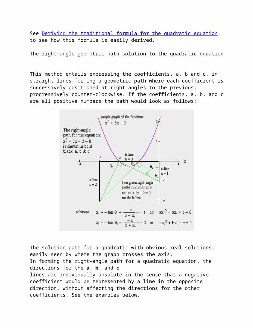
The solution path for a quadratic with obvious real solutions, easily seen by where the graph crosses the axis. In forming the right-angle path for a quadratic equation, the directions for the a, b, and c lines are individually absolute in the sense that a negative coefficient would be represented by a line in the opposite direction, without affecting the directions for the other coefficients. See the examples below.

In general, any algebraic equation can be divided by its first coefficient, so that the first coefficient of the resulting equation is a = +1, without loss in generality. The convention that this author has been using is to begin the a-line vertically, running North by one unit of length, then starting the b-line West, if b is positive, or East, if b is negative from the North end of the a-line by (b/a) units of length. The c-line then proceeds South from the end of the b-line, if c is positive, or North, if c is negative by (c/a) units of length.

This right-angle path method always provides the real solutions where the reduced-paths intersect the b-line, with negative real solutions to the West and positive real solutions to the East, and since the a-line is one unit in length, and the tangent of an angle is the opposite side divided by the right-angle adjacent (=1) the results will be directly measurable in units of length established by the length of the a-line.

The reduced-path is another right-angle path formed between the starting and ending points of the original right-angle path of the equation, but with one less segment in the path. The reduced right-angle path starts at the South end of the a-line, which is also the starting point of the

equation path. Then, it goes toward the b-line and "reflects" from it at a right angle, such that it ends on the open end of the c-line, where the equation path ends. If there are negative coefficients in the equation (i.e. if either c alone or both c and b are negative), then the reduced right-angle path will not intersect directly with the b-line, but instead with its extensions (along the superimposed x-axis in the figure above). In this case the line does not "reflect" but "refracts" at a right angle before continuing as the next example shows.

Generally, there will be several paths, each one corresponding to each real solution of the equation. See the example below.

A deterministic solution circle for quadratic equations

Note that the "reduced path" can be easily found for quadratic equations by forming a circle onto a diameter formed by a straight line connecting the end points of the equation’s path. See the blue circle formed upon the blue diameter shown in the figure below. This circle may intersect the line representing coefficient, b (or its extension), the "b-line", and those points of intersection will be the points along the b-line (or its extension, chosen conveniently to correspond to the x-axis) where the two reduced right-angle paths (shown in green) will be found to touch the b-line and form right angles (See Euclid, The Elements, Book III, Proposition 31). If the circle does not intersect the b-line, nor its extension, then the quadratic equation will have no real solutions. Following this section we will see how to obtain imaginary solutions which occur when the circle does not intersect the b-line (nor its extension) .

A quadratic with its "solution circle". The reader should solve a few quadratic equations with this method to see how easy it is to gain familiarity with it. It is also instructive to show by the geometric laws of similar right triangles, how this method does indeed provide the correct result, consistent with the traditional algebraic formula.

See right angle paths to solve algebraic equations, to see how this right-angle path method is easily demonstrated.

Quadratic Equations with Imaginary Solutions

Fig. 3. Shows a quadratic equation which has complex solutions. The complex solution is found by preparing the right-angle path in the same manner as described above, and then transposing the a-line to add to the c-line as shown in the bold green line in Fig. 3. Then a circle, shown in blue, is constructed with the (c+a)-line as its diameter. The intersection of the blue circle and the b-line (x-axis) determines the radius of the yellow circle which is centered where the b-line (x-axis) intersects the c-line. The value of the imaginary part of the solution to the equation is then given by the vertical distance along the x = - b/2 line between the b-line and its intersection with the yellow circle. In figure 3, this distance is shown as a fine dotted purple line that extends above and below the b-line along the x = - b/2 line by an amount equal to the imaginary term of the complex solution to the quadratic equation.

The demonstration that the above construction is valid is shown by simple theorems in plane geometry. It’s important to realize that it is not necessary to plot the equation: y = ax2 + bx + c in order to perform the geometric solution. A quick look at the diagram, will confirm that the imaginary part of the complex solution is equal to the square root of the vertical distance between the minimum point of the curve and the x-axis, which is another way to visualize the complex solution.

Fig. 3, A quadratic example with two deterministic solution circles, showing how to find its complex solutions.

Once the reader is satisfied that the method is valid, then it is safe to proceed to cubic equations (n = 3), and higher order equations. In quadratic equations, there is an easy deterministic (i.e. ruler and compass, geometrically "exact" solution) as illustrated by the solution circle method. However, for cubic and quartic equations (n = 3 and n = 4) such deterministic ruler and compass methods may exist if markings are allowed on the ruler, but are not convenient to use. For quintic (n = 5) and higher degree equations, in the general case, it is almost certain that no geometrically deterministic exact solution is possible.

However, using a transparent graph paper with perpendicular fine lines overlaid on top of an equation path, one can gradually rotate the transparent graph paper to find approximate solutions for equations of any degree.

The basic rules are the same for equations of any degree. The reduced right-angle paths provide the real solutions on the b line, negative ones to the West and positive ones to the East. The reduced path reflects at right angles on each of the equation lines in order, or refracts from their extensions. For equations of odd degree (n = 3,5,7, etc.) there is always one real solution. For equations of even degree (n = 2,4,6, etc.), there may be no real solution. But, if there are, they will occur in pairs.

The reduced right-angle path is also a right-angle path for the reduced equation, once the solution provided by the reduced path is "divided out" of the original equation.

See the Quadratic Equation Applet and the Complex Quadratic Solution Applet in the description of available Applets.

Editorial Note: The applications of the applets are reasonably well-described in the linked document which is the Word (docx) equivalent of an html form document requiring Java and a third party add-on that is not readily available for current browsers. Between the comments in this section of the website and those in the Word forms for on the associated applets, it is hoped that the geometric processes for each solution process will be evident.

The Cubic Equation (n = 3)

The cubic equation is usually presented as follows:

An algebraic solution for cubic equations is found in many references on algebra, such as Carl Pearson’s Handbook of Applied Mathematics, published by Van Nostrand Reinhold. However, the algebraic solution is complicated and is usually not represented by one single equation, but rather by a sequence of equations with intermediary values, some of which are complex numbers. This link shows some of the traditional methods of algebraically solving a cubic equation. The traditional solutions are not easy to remember and difficult to re-derive. In actual practice it is more common for cubic equations to be solved by graphical means using graphical calculators or desktop graphical calculator programs on personal computers. Using the right-angle path method for solving a simple cubic equation is illustrated in Fig. 4, below:

Fig. 4, an example of a cubic equation.

In the example of Fig. 4, the red right-angle subpath reflects off of the b-line at x = - 1, providing that solution to the cubic equation. The red path also represents a quadratic equation with roots at x = -2 and x = -3. The yellow solution circle intersects the "b-line" of the red quadratic path at distances 2 and 3 times its first leg (a-line). Likewise, the blue right-angle subpath, provides the solution x = -2 from where it reflects on the b-line of the cubic equation. The blue quadratic path intersects with the "b-line" of the blue path at 1 and 3 times the length of its a-line, thus representing the solution X = -1 and x = -3. Similarly, the green quadratic subpath shows the solution, x = -3 from its reflection of the cubic b-line, and its intersections with the "b-lime" of the green path and the yellow circle are at 1 and 2 times the length of its a-line.

Thus, as this example shows, each of the three solution subpaths provides, sequentially, the remaining two solutions, and the remaining two solution paths can also be found directly.

For a cubic equation, once one solution is found, it is easy to know whether or not the remaining two are real or complex by constructing the solution circle and seeing if it intersects with the b-line of the subpath quadratic. If it does intersect (as in the example of Fig. 4) there will be other real solutions (as are shown), if it does not intersect, then the remaining two solutions are complex.

In the following example, shown in Fig. 5, a cubic equation is shown where the coefficient, d, is negative. In this equation, the red solution path, and the yellow solution sub-path, form sub-paths that represent quadratic equations with a negative coefficient that (therefore) has two real roots, therefore the cubic equation has three real roots.

Fig. 5

If one were to decrease the coefficient, d, in the above example of a cubic equation (extending the d-line farther to the left), then at some point, such as d < -5, it becomes impossible for a red path, or a yellow sub-path to be constructed. At some larger negative value of d, there will only be a sub-path of the type shown in green. And, as a quadratic sub-path the green path would represent a quadratic equation with the remaining two solutions. However, the solution circle for the green path would show that it does not have real solutions, because the solution circle would not intersect the central arm (b-line) of the green path. Thus, one can "see" that the cubic equation will have only one real solution as the value of d decreases below a certain level, such as d < -5 (the other two will be complex conjugates).

This method of right-angle path solutions to algebraic equations offers the ability to quickly "see" the relative magnitudes, signs, and whether on not the solutions are real or complex.

See Cubic Equation Applet.

Reversing the path and the reverse equation.

One interesting facet of the right-angle path method of solving algebraic equations, is the reversibility of the right-angle paths and the equations. This may be illustrated on the examples of the cubic equations used in Fig. 4 and Fig. 5, above. Additionally, the reversible quality is true for equations of any degree.

Consider first the equation and right-angle path for the cubic equation of Fig. 1:

The equation is:

Now rotate the Figure clockwise by 90 degrees. Then the right-angle path can be seen as beginning with the d-line (6 units long) and ending on the a-line (one unit long). As a right-angle path, the black bold lines now show the reverse equation:

The reverse equation has reversed coefficients, and certain sign changes compared to its original. These sign changes depend upon the geometric directions of the right-angle path.

Note that the solutions, as the negative tangents of the angles between the sub-paths and the equation path, are opposite in sign from those of the original equation and are fractions with 6 as the denominator. From the rules of similar triangles one can quickly conclude that the solutions of the reverse equation are the negative reciprocals of those of the original equation. This result is true for equations of any degree.

Consider next the equation and right-angle path for the cubic equation of Fig. 4:

The equation is:

Now, rotate the Figure counter-clockwise by 90 degrees. Then the right-angle path can be seen as beginning with the d-line and ending on the a-line. Thus, it becomes a different and reversed equation, but the right-angle subpath again remains the same as for the original equation.

The reverse equation is:

which has its coefficients reversed and two sign changes compared to the original equations. The solutions for the reverse equation are found on its a-line, which is the c-line for the original equation. Again the solutions for the reverse equation are the negative inverses of the solutions for the original equation. This is a general result. In summary:

Fig. 6, Reverse paths and negative inverse solutions.

Of course, the same result is obtained when one algebraically replaces x with -(1/x) in any such algebraic equation. However the right-angle path method enables one to "see" the reverse equation in the same diagram.

Some degenerate cases.

If the first coefficient of an algebraic equation is zero, the equation reduces to one of a lesser degree, and can be treated accordingly. If the last coefficient is zero, then one solution is x = 0 and the balance of the equation, once it is divided by x, is one of lesser degree, and it can be treated accordingly.

When intermediate coefficients are zero, then the right-angle path still works by working with the extension of the line on which the coefficient falls, even though it has a zero value. The following illustration shows how to deal with a cubic equation which has a zero coefficient in the squared term.

Fig. 7, Cubic with no squared term.

A very interesting case is to look at right-angle paths when all of the intermediate coefficients are zero. That is:

Where r is any real positive number, and n is any positive integer. This is the simple equation solved by x = the nth root of r. The right-angle path method provides a visual way to observe any root of any positive real number. The following illustration shows some simple examples of the right-angle path relationships between any positive real number and its powers and roots. Note that the finding of the cube root of 2 using right angle paths solves the famous historic problem known as "doubling the cube", that is, finding a length that when cubed produces a cube that has twice the volume of a given cube.

Fig. 8, Roots and powers.

See Applet for Geometric Visualizatioccn of a Cube Root.

Closed Right-Angle Paths, and their equations. An interesting class of algebraic equations is formed by starting with a general equation of order n and multiplying it by

The resulting algebraic equation will be of order n + 2 and will have the same roots as the original equation of order n, and two additional roots which are: x = +/- i, where i is the square root of - 1, the unit imaginary number.

The resulting equation, of order n + 2 will form a right-angle path which is closed, that is, the beginning and end of the equation are at the same point. This is easily shown from the fact that the sum of the coefficients for the even and odd powers, respectively, with signs alternated, is zero. Thus, the solution paths will also be closed, creating some interesting geometric figures for visualizing solutions to the original equation.

Another consequence of closed-path equations is that the quadratic solution circle for the quadratic remaining after n solution subpaths are sequentially revealed, degenerates to a single point, the common starting and ending point with zero radius. This corresponds to the right-angle path for

which is a straight line that folds back upon itself, with no b-line, and its starting point the same as its ending point. It will show up as the diagonal of a rectangle, with the starting and ending point at one of its corners, representing a closed-path cubic.

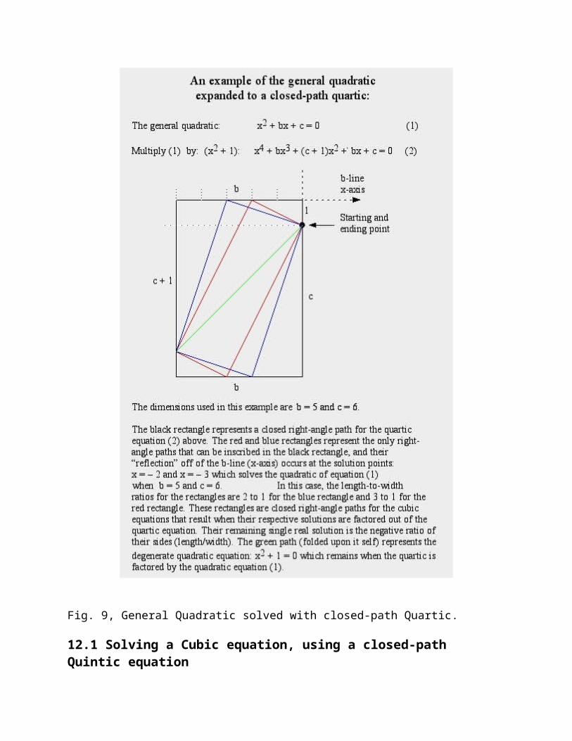
In the figure below, an example of a general quadratic equation is multiplied by

to obtain a quartic or 4th degree equation, with the same real roots as the quadratic equation, and it forms a closed right-angle path.

In this example, and in those which follow, the first term, a, is set to a = 1 without any loss of generality. By making this selection, the b-line corresponds with the negative x-axis and the solutions all appear along the x-axis.

Also, in this example, and in those which follow, the coefficients are selected to be positive numbers for convenience. The technique will also work with negative coefficients, sometimes resulting in different geometric figures, however, the expanded "n + 2" equation path will still always be a closed path, regardless of the sign of the coefficients.

Fig. 9, General Quadratic solved with closed-path Quartic.

12.1 Solving a Cubic equation, using a closed-path Quintic equation

The following figure shows how a general cubic equation (n = 3) can be expanded to closed-path quintic equation (n = 5).

Fig. 10, General Cubic solved with closed-path Quintic.

It is especially important to note that the expansion to closed-path equations with power n + 2 to solve general equations with power n, provides convenient closed path geometric figures that

may be easier to visualize than open ended paths. In the use of drafting equipment, or transparent graph paper, changes in the closed figures, as the coefficients are changed, are easier to visualize.

In the example of Fig. 10, the solutions to the cubic equation (1) are found where each of the red, blue, and green closed path quartics reflect from the b-line (x-axis). These solutions are: x = - 1, x = -3, and x = -4 for the coefficients selected, i.e. a = 1, b = 8, c =19, and d = 12. Thus, the cubic becomes (x + 1)(x + 3)(x + 4) = 0

It is also evident in the example of Fig. 10, that each of the red, blue, and green quartic closed subpaths can be solved for the two roots that they do not represent. Since the blue and green paths are geometric squares (but represent cubic equations), one can easily see that they are each solved by an enclosed closed-path cubic square, whose corner rests on the starting and ending point. The other solution for each of these geometric squares is a rectangle formed at a 45 degree angle (these rectangles represent the x = -1 solution). The red path is solved by two rectangles; one, which has the length to width ratio of 3 to 1, and the other 4 to 1.

The point to consider is that a cubic equation can be solved using the expanded closed-path quintic and extracting one real root by finding a quartic sub-path and sequentially extracting other real roots (if there are any) from that closed-path quartic, or by extracting 3 real roots by finding 3 quartic subpaths. So, roots can be extracted both sequentially, and in parallel.

12.2 Trisecting an angle with right-angle paths

It has long been known that an arbitrary angle cannot be trisected with an unmarked straight edge and compass alone. It is also known that trisecting an angle involves solving a cubic equation. The history of this problem and many of the geometric means (using marked straight edges and conics) are shown on the web page Trisecting an Angle by J. J. O’Conner and E. F. Robertson.

Trisecting an arbitrary angle can also be done with right-angle paths as shown in Fig. 11. This solution is not particularly elegant, and provides no deterministic solution by unmarked straight-edge and compass, but the solution can be provided "mechanically" by the rotation of transparent graph paper over a deterministic diagram.

Fig. 11, Trisecting an angle with right-angle paths.

In Fig. 11, the cubic equation is derived from the formula for the tangent of the triple of an arbitrary angle given in many trigonometric references. See, for example. Tables of Integrals and Other Mathematical Data by H. B. Dwight. That cubic equation is then converted to a closed-path quintic equation using the techniques described earlier on this web page. The closed path quintic equation is presented in Fig. 10 in a position rotated clockwise by 90 degrees to conform to the related diagram associated with a much older method of trisecting an angle which was known to Hippocrates (c470-410 B.C.).

Referring to Fig. 11, the method known to Hippocrates requires finding a line from points A to E, such that CG = HG = GE = AC. This line cannot be made deterministically except by allowing two points marked on a straight-edge separated by a distance of 2AC to be "slid" along the lines CE and CD until the straight edge also touches the point A.

The red right-angle paths shown in Fig. 11 also results in finding the same point at E, but in a non-related manner. While the right-angle path method of trisecting an angle is more cumbersome and less elegant, it does show that its level of mechanical determinism, at least for cubic equations, is no less that which can be solved with a marked straight-edge and compass. Since the right-angle path method can be used for equations of any degree, the concept of a set of mechanically continuously adjustable and rotatable rectangles may provide the ultimate geometric tool for complete geometric determinism.

This web page is under construction, with the following sections to be added soon:

Right-angle path solutions to quartic equations. Right-angle path solutions to quintic equations. Right-angle path solutions to sextic and septic equations. Right-angle path solutions to very high order equations. Right-angle path solutions to equations of infinite degree. Synthesis of algebraic equations with known roots using the Right-angle path method.

Editorial note: Sadly the author died before completing these sections. They remain as a challenge to interested readers.